Electroweak couplings and LHC constraints
on alternative $Z^{\prime}$ models in $E_{6}$

Abstract

We report the most general expression for the chiral charges of a $Z^{\prime}$ gauge boson coming from an $E_{6}$ unification model, as a function of the electroweak parameters and the charges of the $U(1)$ factors in the chain of subgroups. These charges are valid for an arbitrary Higgs sector and only depend on the branching rules of the $E_{6}$ fundamental representation and the corresponding rules for the fermionic representations of their subgroups. By assuming $E_{6}$ unification, the renormalization group equations (RGE) allow us to calculate the electroweak parameters at low energies for most of the chains of subgroups in $E_{6}$. From RGE and unitary conditions, we show that at low energies there must be a mixing between the gauge boson of the standard model hypercharge and the $Z^{\prime}$. From this, it is possible to delimit the preferred region in the parameter space for a breaking pattern in $E_{6}$. In general, without unification, it is not viable to determine this region; however, for some models and under certain assumptions, it is possible to limit the corresponding parameter space. By using the most recent upper limits on the cross-section of extra gauge vector bosons $Z^{\prime}$ decaying into dileptons from the ATLAS data at 13 TeV with accumulated luminosities of 36.1 fb^-1 and 13.3 fb^-1, we report the 95$\%$ C.L. lower limits on the $Z^{\prime}$ mass for the typical $E_{6}$ benchmark models. We also show the contours in the 95% C.L. of the $Z^{\prime}$ mass bounds for the entire parameter space of $E_{6}$.

PACS numbers:

1 Introduction

From a group theory point of view, there are several ways to break the $E_{6}$ symmetry down to the standard model (SM) one. Although some of the breaking patterns have been explored in the literature so far, a systematic study of the phenomenology for all the alternative ways has not been done as far as we know. In general, intricate models are not appealing. A way to look for new models with a moderate fermion content is to consider alternative versions of the models already known in the literature [1, 2, 3, 4, 5, 6, 7, 8, 9, 10]. Our work represents a first step in this direction. One of the first alternative models was “flipped $SU(5)$” [1, 11], which produces a symmetry breaking for $SO(10)$ down to $SU(5)\otimes U(1)$, where the $U(1)$ factor contributes to the electric charge, and as such, its basic predictions for $\sin^{2}\theta_{W}$ and the proton decay are known to be different from those of $SU(5)$ [1]. An alternative model for the flipped $SU(5)$ is $SO(10)\otimes U(1)_{N}$, where the right-handed neutrino has zero charge under the $U(1)_{N}$ group allowing a Majorana mass term [5, 12]. The alternative versions of the left-right model are also well known in the literature [4, 13], as in the latter case, one of these models allows for a right-handed neutrino component effectively inert [4].

The alternative models have been useful in the study of the grand unified theories (GUTs) phenomenology, for example, for the $E_{6}$ subgroup $SU(2)_{R}\otimes SU(6)$ and some of its three alternative versions, the gauge mediated proton decay operators are suppressed at leading order due to the special placement of matter fields in the unified multiplets [14, 15, 16, 17, 9, 18].

Heavy neutral gauge bosons are a generic prediction of many types of new physics beyond the SM. In addition, these extra $U(1)^{\prime}$ symmetries serve as an important model-building tool [19] (for example, to suppress strongly constrained processes) giving rise, after spontaneous $U(1)^{\prime}$ symmetry breaking, to physical $Z^{\prime}$ vector bosons. Thus, with the upgrade of the luminosity and the energy of the LHC, there exists a real possibility for the on-shell production of a $Z^{\prime}$ boson [20, 21].

All representations of the $E_{6}$ gauge group [22, 23] are anomaly-free and the fundamental 27-dimensional representation is chiral and can accommodate a full SM fermion generation. As a consequence, $E_{6}$-motivated $Z^{\prime}$ bosons arise naturally in many popular extensions of the SM [20, 2, 24, 25], both in top-down and bottom-up constructions. Some of the $E_{6}$ subgroups, such as the original unification groups $SU(5)$ and $SO(10)$, and the gauge group of the left-right symmetric models $SU(4)_{C}\otimes SU(2)_{L}\otimes SU(2)_{R}$, play central roles in some of the best motivated extensions of the SM. Furthermore, the complete $E_{6}$-motivated $Z^{\prime}$ family of models appears in a supersymmetric bottom-up approach exploiting a set of widely accepted theoretical and phenomenological requirements [26]. The one-parameter $Z^{\prime}$ families in reference [27], denoted as ${\bf 10}+x{\bf\bar{5}}$, $d-xu$ and $q+xu$, where ${\bf 10}$ and ${\bf\bar{5}}$ are $SU(5)$ representations, can also be discussed within the $E_{6}$ framework [28].

For all these reasons there is an expectation that an $E_{6}$ Yang-Mills theory, or a subgroup of $E_{6}$ containing the SM in a non-trivial way, might be part of a realistic theory [29]. If a heavy vector boson is seen at the LHC or at an even more energetic collider in the future, aspects of the $E_{6}$ symmetry group will be central to the discussion of what this resonance might be telling us about the fundamental principles of nature.

The discrimination between $Z^{\prime}$ models could be challenging at the LHC due to the small number of high resolution channels at hadron colliders. Another reason why the determination of the underlying symmetry structure is not straightforward is that the mass eigenstate of the $Z^{\prime}$ is, in general, a linear combination of some of the underlying $Z^{\prime}$ charges with the ordinary $Z$ boson of the SM. Hence, it is useful to reduce the theoretical possibilities or at least to have a manageable setup. This work represents an attempt in this direction and serves to spotlight a few tens of models in the two-dimensional space of $E_{6}$-motivated $Z^{\prime}$ models.

All the $E_{6}$ breaking patterns and branching rules have been tabulated in Ref. [29]. In references [2, 7] all the chains of subgroups were tabulated. The aim of the present work is to set the impact of the latest LHC constraints on the possible embeddings of the SM in the subgroups of $E_{6}$.

It is important to remark that many interesting phenomenological models appear in a natural way in $E_{6}$ breaking patterns, such as the proton-phobic, $Z_{\not{p}}$, neutron-phobic, $Z_{\not{n}}$, (vector bosons which at zero momentum transfer do not couple to protons and neutrons, respectively), leptophobic $Z_{\not{L}}$ (with zero couplings to leptons) and vector bosons from supersymmetric models, as for example the $Z_{N}$ model [5, 12], etc. We will show a more complete list later.

The study reported here is a continuation of the analysis started in Ref. [7] where the quantum numbers of the abelian gauge groups in alternative chains of subgroups of $E_{6}$ were calculated. Several of the subgroups shown there are well known in the literature; however, as far as we know, the phenomenology of many of these models have not been studied. Of particular importance for the electroweak constraints are the $Z^{\prime}$ chiral charges of the SM fermions which depend on the chosen chain of subgroups. In the present work, we show the general expression for these charges and determine the preferred region in the parameter space for some breaking patterns. We also establish that the mixing between the $Z^{\prime}$ charges and the SM hypercharge is a measure of the deviation of the parameter space at low energies respect to their unification values. We demonstrate that the presence of this mixing stems from the gauge coupling splitting at low energies.

The paper is organized as follows: In Section 2 we derive general expressions for the electroweak (EW) charges of a $Z^{\prime}$ in $E_{6}$ as a function of the mixing angles and the charges of an arbitrary $U(1)$ in $E_{6}$. In section 3 we show that even for a group with orthonormal charges at low energies there is a kinetic mixing due to the splitting of the gauge coupling constants. In section 4 we revise the existing literature about models based on $E_{6}$ subgroups and their embeddings. By assuming $E_{6}$ unification the renormalization group equations (RGE) allow us to determine the parameter space of the $Z^{\prime}$ associated with some of these models. For this purpose, we take the expressions for the mass scales and couplings of the Robinett and Rosner (RR) work [2]. In this section, we also point out the existence of non-trivial models which, to the best of our knowledge, have not been studied in the literature. In section 5 we delimit the parameter space when we put aside the unification hypothesis as it usually happens for effective models at low energies. In section 6 the 95% C.L. exclusion limits on the neutral boson masses for the entire $E_{6}$-motivated $Z^{\prime}$ parameter space are shown.

2 General expressions

Owing to the fact that the rank of $E_{6}$ is 6, for chains of subgroups with regular embeddings (those preserving the rank) the most general form of the group associated with the low-energy effective model is [29, 2] $SU(3)_{C}\otimes SU(2)_{L}\otimes\prod_{\kappa}U(1)_{\kappa}$, with $\kappa=a,b,c$; where the $U(1)$ factors come from the chains of subgroups of $E_{6}$. In order to reproduce the $SU(3)_{C}\otimes SU(2)_{L}\otimes U(1)_{Y}$ symmetry of the SM it is necessary that the SM hypercharge $Y$ be a linear combination of the $U(1)_{k}$ charges $Q_{\kappa}$. If $g$ is the $SU(2)_{L}$ coupling constant and $A^{\mu}_{3L}$ the gauge boson associated with the third component of the weak isospin, then the neutral current Lagrangian $\mathcal{L}_{NC}$ for the most general case is

$$-\mathcal{L}_{NC}=gJ^{\mu}_{3L}A_{3L\mu}+g_{a}J^{\mu}_{a}A_{a\mu}+g_{b}J^{\mu}_{b}A_{b\mu}+g_{c}J^{\mu}_{c}A_{c\mu}\ ,$$ (1)

where $g_{\kappa}$ and $A^{\mu}_{\kappa}$ represent the gauge coupling constant and the gauge field associated with the $U_{\kappa}(1)$ symmetry, respectively. The fermion currents $J^{\mu}_{\kappa}$ are given by

$$J^{\mu}_{\kappa}=\sum_{f}\overline{f}\gamma^{\mu}[\epsilon_{L}^{\kappa}(f)P_{L}+\epsilon_{R}^{\kappa}(f)P_{R}]f,$$ (2)

where $f$ runs over all fermions in the ${\bf 27}$ representation of $E_{6}$, which is the fundamental representation. The chirality projectors are defined as usual i.e., $P_{L,R}=(1\pm\gamma^{5})/2$ and $f_{L,R}=P_{L,R}f$. The chiral charges are $\epsilon_{L}(f)=Q_{k}(f_{L})$ and $\epsilon_{R}(f)=-Q_{k}(f^{c}_{L})$. The $U(1)_{\kappa}$ charges satisfy the $E_{6}$ normalization condition $\sum_{f\in\mathbf{27}}Q^{2}_{\kappa}(f)=3$ (see Table D in appendix D). As a consequence of this, the electric charge operator $Q_{em}$ is given by

$$Q_{em}=T_{3}+Y=T_{3}+\sqrt{\frac{5}{3}}Q_{Y}^{E_{6}}\ ,$$

where $T_{3}$ is the third component of weak isospin and $Q_{Y}^{E_{6}}$ is the $E_{6}$ normalized SM hypercharge.

By means of an orthogonal transformation $\mathcal{O}$ we can pass from the gauge interaction basis to the basis in which one of the fields can be identified with the SM hypercharge $B^{\mu}$ associated with the $U(1)_{Y}$ symmetry. If we define such a rotation through 

$$\begin{pmatrix}A^{\mu}_{3L}\\ A^{\mu}_{a}\\ A^{\mu}_{b}\\ A^{\mu}_{c}\end{pmatrix}=\mathcal{O}\begin{pmatrix}A^{\mu}_{3L}\\ B^{\mu}\\ Z^{\prime\mu}\\ Z^{\prime\prime\mu}\end{pmatrix}=\begin{pmatrix}1&0&0&0\\ 0&O_{11}&O_{12}&O_{13}\\ 0&O_{21}&O_{22}&O_{23}\\ 0&O_{31}&O_{32}&O_{33}\end{pmatrix}\begin{pmatrix}A^{\mu}_{3L}\\ B^{\mu}\\ Z^{\prime\mu}\\ Z^{\prime\prime\mu}\end{pmatrix}\ ,$$ (3)

then the Lagrangian (1) can be written as

$$-\mathcal{L}_{NC}=gJ^{\mu}_{3L}A_{3L\mu}+g_{Y}J^{\mu}_{Y}B_{\mu}+g_{Z^{\prime}}J_{Z^{\prime}}^{\mu}Z^{\prime}_{\mu}+g_{Z^{\prime\prime}}J_{Z^{\prime\prime}}^{\mu}Z^{\prime\prime}_{\mu}\ .$$ (4)

In order to keep invariant the Lagrangian, the currents must transform with the same orthogonal matrix

$$g_{Y}J^{\mu}_{Y} =g_{a}J^{\mu}_{a}O_{11}+g_{b}J^{\mu}_{b}O_{21}+g_{c}J^{\mu}_{c}O_{31}\ ,$$ (5)

$$g_{Z^{\prime}}J_{Z^{\prime}}^{\mu} =g_{a}J^{\mu}_{a}O_{12}+g_{b}J^{\mu}_{b}O_{22}+g_{c}J^{\mu}_{c}O_{32}\ ,$$ (6)

$$g_{Z^{\prime\prime}}J_{Z^{\prime\prime}}^{\mu} =g_{a}J^{\mu}_{a}O_{13}+g_{b}J^{\mu}_{b}O_{23}+g_{c}J^{\mu}_{c}O_{33}\ .$$ (7)

The exact expression for the orthogonal matrix is given in appendix A. In order to obtain the SM as an effective theory at low energies, the breaking $U_{a}(1)\otimes U_{b}(1)\otimes U_{c}(1)\longrightarrow U(1)_{Y}$ must take place. If so, it is possible to find three real coefficients $k_{a}$, $k_{b}$ and $k_{c}$ such that

$$Y=\sqrt{\frac{5}{3}}Q_{Y}^{E_{6}}= k_{a}Q_{a}+k_{b}Q_{b}+k_{c}Q_{c}\ .$$ (8)

From Eqs. (2) and (8) we obtain for the currents the relation

$$J_{Y}^{\mu}=k_{a}J_{a}^{\mu}+k_{b}J_{b}^{\mu}+k_{c}J_{c}^{\mu}\ .$$ (9)

In Tables D to D (in appendix D) we have reported the values of $k_{\kappa}$ for the models considered in this work. By comparing Eq. (9) with Eq. (5), we get the following expressions:

$$g_{a}O_{11}=k_{a}g_{Y}\ ,\hskip 14.22636ptg_{b}O_{21}=k_{b}g_{Y}\ ,\hskip 14.22636ptg_{c}O_{31}=k_{c}g_{Y}\ ,$$ (10)

which, along with the orthogonal condition $O_{11}^{2}+O_{21}^{2}+O_{31}^{2}=1$, impose a constraint on the $g_{a}$, $g_{b}$ and $g_{c}$ coupling constants, namely:

$$\left(\frac{k_{a}}{g_{a}}\right)^{2}+\left(\frac{k_{b}}{g_{b}}\right)^{2}+\left(\frac{k_{c}}{g_{c}}\right)^{2}=\left(\frac{1}{g_{Y}}\right)^{2}\ .$$ (11)

From these expressions and the explicit form of the rotation matrix $\mathcal{O}$ (see A) we get the $Z^{\prime}$ chiral charges (see B)

$$g_{Z^{\prime}}\epsilon^{Z^{\prime}}_{L,R}= \ \ \ A_{L,R}\cos\theta+B_{L,R}\sin\theta\ ,$$ (12)

$$g_{Z^{\prime\prime}}\epsilon^{Z^{\prime\prime}}_{L,R}= -A_{L,R}\sin\theta+B_{L,R}\cos\theta\ ,$$ (13)

where

$$A_{L,R}= \hskip 8.5359pt\frac{g_{c}}{\hat{\alpha}_{c}}\left(\dfrac{k_{a}\epsilon^{b}_{L,R}}{\hat{\beta}}-\hat{\beta}k_{b}\epsilon^{a}_{L,R}\right),$$ (14)

$$B_{L,R}= g_{Y}\left(-\dfrac{k_{a}\epsilon^{a}_{L,R}+k_{b}\epsilon^{b}_{L,R}}{\hat{\alpha}_{c}}k_{c}+\hat{\alpha}_{c}\epsilon^{c}_{L,R}\right)\ ,$$ (15)

and $\theta$ is an angle of the rotation matrix $\mathcal{O}$ which can take any value between $-\pi$ and $\pi$. Here $\hat{\alpha}_{c}=g_{c}\sqrt{\frac{k_{a}^{2}}{g_{a}^{2}}+\frac{k_{b}^{2}}{g_{b}^{2}}}=\sqrt{\frac{g_{c}^{2}}{g^{2}}\cot^{2}\theta_{W}-k_{c}^{2}}$, and $\hat{\beta}=\frac{g_{a}}{g_{b}}$. In order to have the chiral charges properly normalized in $E_{6}$ we define

$$g_{Z^{\prime}}\equiv \frac{1}{{\hat{\alpha}_{c}\hat{\beta}}}\bigg{(}\cos^{2}\theta g_{c}^{2}(k_{a}^{2}+\hat{\beta}^{4}k_{b}^{2})-2\hat{\beta}(1-\hat{\beta}^{2})g_{c}g_{Y}k_{a}k_{b}k_{c}\cos\theta\sin\theta$$ (16)

$$+\hat{\beta}^{2}g^{2}_{Y}\left((k_{a}^{2}+k_{b}^{2})k_{c}^{2}+\hat{\alpha}_{c}^{4}\right)\sin^{2}\theta\bigg{)}^{1/2}\ ,$$ (17)

which reduces to the Georgi-Glashow well known result $\sqrt{\frac{5}{3}}g_{Y}=\sqrt{\frac{5}{3}}g\tan\theta_{W}$ for $g_{c}=g_{a}=g_{b}$. These charges reproduce the electroweak charges of trinification and the left-right symmetric model which are well known in the literature (for additional references look into our previous work [13]). Since $g_{Z^{\prime}}\epsilon^{Z^{\prime}}_{L,R}(\theta+\pi/2)=g_{Z^{\prime\prime}}\epsilon^{Z^{\prime\prime}}_{L,R}(\theta)$, the parameter space associated with the $Z^{\prime\prime}$ boson is the same as that of the $Z^{\prime}$ boson.

3 Kinetic mixing from gauge coupling splitting

Because all the generators $Q_{ij}^{a}$ associated with the neutral currents can be diagonalized simultaneously the corresponding fields can be written as $A^{\mu}=A^{\mu a}T^{a}_{ij}=A^{\mu a}Q^{a}(i)\delta_{ij}$, where $Q^{a}(i)$ stands for the charge of the $i$-fermion in the fundamental representation. For these fields the most general lagrangian is given by

$$\text{Tr}[F_{\mu\nu}F^{\mu\nu}]= \text{Tr}[F_{\mu\nu}^{a}T^{a}F^{\mu\nu b}T^{b}]$$

$$F_{\mu\nu}^{a}F^{\mu\nu b}\sum_{i,j}Q^{a}(i)\delta_{ij}Q^{b}(j)\delta_{ji}= F_{\mu\nu}^{a}F^{\mu\nu b}\sum_{i}Q^{a}(i)Q^{b}(i).$$ (18)

When $i$ runs over the fermions in a multiplet of a simple group (or a semisimple group that comes from the breaking of a simple Lie group) the charges are orthonormal

$$\sum_{i}Q^{a}(i)Q^{b}(i)=\sum_{i}\epsilon^{a}(i)\epsilon^{b}(i)=\delta_{ab}\ .$$ (19)

It is not possible to generate a kinetic mixing term to tree level because $F^{\mu\nu a}$ transforms with an orthogonal matrix; however, at low energies it is possible to generate a kinetic mixing by one-loop corrections [31, 32, 33, 20]. As we will show, a source of kinetic mixing at low energies is the splitting of the values of the coupling strengths. By unitarity the currents should transform in the same way as the fields; if we transform from the group basis to a basis where one of the fields corresponds to the vector field associated with the SM hypercharge $B_{\mu}$, the corresponding expression for the currents is

$$\begin{pmatrix}gJ^{\mu}_{3L}\\ g_{Y}J^{\mu}_{Y}\\ g_{Z^{\prime}}J^{\prime\mu}\\ g_{Z^{\prime\prime}}J^{\prime\prime\mu}\end{pmatrix}\ =\mathcal{O}^{T}\begin{pmatrix}gJ^{\mu}_{3L}\\ g_{a}J^{\mu}_{a}\\ g_{b}J^{\mu}_{b}\\ g_{c}J^{\mu}_{c}\end{pmatrix}=\begin{pmatrix}1&0&0&0\\ 0&O_{11}&O_{12}&O_{13}\\ 0&O_{21}&O_{22}&O_{23}\\ 0&O_{31}&O_{32}&O_{33}\end{pmatrix}^{T}\begin{pmatrix}gJ^{\mu}_{3L}\\ g_{a}J^{\mu}_{a}\\ g_{b}J^{\mu}_{b}\\ g_{c}J^{\mu}_{c}\end{pmatrix}\ .$$ (20)

From the definitions $g_{Y}J_{Y}^{\mu}(f)=\sum_{\kappa}\mathcal{O}_{1\kappa}g_{\kappa}J_{\kappa}^{\mu}(f)$ , $g_{Z^{\prime}}J_{Z^{\prime}}^{\mu}=\sum_{\lambda}\mathcal{O}_{2\lambda}g_{\lambda}J_{\lambda}(f)^{\mu}$, and the Eq. 2 we obtain the expressions

$$g_{Y}Y= \sum_{\kappa}\mathcal{O}_{1\kappa}g_{\kappa}\epsilon^{\kappa}(f)\ ,$$ (21)

$$g_{Z^{\prime}}\epsilon_{Z^{\prime}}= \sum_{\lambda}\mathcal{O}_{2\lambda}g_{\lambda}\epsilon^{\lambda}(f)\ .$$ (22)

By taking the dot product of the SM hypercharge $gY$ and the $Z^{\prime}$ charges $g_{Z^{\prime}}{\bm{\epsilon}}_{Z^{\prime}}$ we obtain

$$g_{Y}{\bf Y}\cdot g_{Z^{\prime}}{\bm{\epsilon}}_{Z^{\prime}}\equiv \sum_{f\in 27}g_{Y}Y(f)g_{Z^{\prime}}\epsilon_{Z^{\prime}}(f)$$

$$= \sum_{\kappa,\lambda}\sum_{f\in 27}\mathcal{O}_{1\kappa}g_{\kappa}\epsilon^{\kappa}(f)\mathcal{O}_{2\lambda}g_{\lambda}\epsilon^{\lambda}(f)$$ (23)

$$= 3\sum_{\kappa}\mathcal{O}_{1\kappa}\mathcal{O}_{\kappa 2}^{T}g_{\kappa}^{2}\ ,$$ (24)

where $\mathcal{O}$ is the rotation matrix (3). Here we made use of the $E_{6}$ orthonormality relation $\sum_{f\in 27}\epsilon^{\kappa}(f)\epsilon^{\lambda}(f)=3\delta_{\kappa\lambda}$ between the $U(1)_{\kappa}$ charges that come from a chain of subgroups. By assuming that the three couplings are identical $g_{a}=g_{b}=g_{c}$ we obtain $g_{Y}{\bf Y}\cdot g_{Z^{\prime}}{\bm{\epsilon}}_{Z^{\prime}}=3g_{a}^{2}\sum_{\kappa}\mathcal{O}_{1\kappa}\mathcal{O}_{\kappa 2}^{T}=3g_{a}^{2}\delta_{12}=0$, otherwise

$${\bf Y}\cdot{\bm{\epsilon}}_{Z^{\prime}}=\sum_{f\in 27}Y(f)\epsilon_{Z^{\prime}}(f)\neq 0\ .$$ (25)

Figure 1: $Z_{\mu}^{\prime}$-$B_{\mu}$ kinetic mixing.

This result shows that the orthonormality of the SM hypercharge and the $Z^{\prime}$ charges is only guaranteed when all the three couplings are equal as it happens in unification; for the remaining cases a kinetic mixing is generated by the one-loop diagram in figure 1 (even for complete fermion representations).

In general, at low energies the gauge couplings $g_{\kappa}$ are different each other due to the RGE; thus, as will be shown below, the $Z^{\prime}$ charges associated with a chain of subgroups in $E_{6}$ are no longer orthonormal to the SM hypercharge. It is important to notice that the 2-loop corrections are important for the RGE since they modify in a considerable way the mass unification scales; however, for several models, unification does not impose relations between the SM electroweak couplings in such a way that the consistency of the model does not depend on high order corrections and the SM values for the $\alpha_{i}=g_{i}^{2}/(4\pi)$ can be considered as input parameters. Under these conditions, the 1-loop coupling strengths [2] $g_{\kappa}$ associated to the extra $U(1)$ abelian symmetries differs in just a few percent respect to the 2-loop result at the electroweak scale, since the bondary condition on the SM parameters is imposed at the same energy scale [34].

The phenomenological consequences of the $B_{\mu}-Z_{\mu}^{\prime}$ kinetic mixing is a modification of the $Z$ charges [32, 33, 20]. In turn, this contribution represents a non-zero value for the $Z\text{-}Z^{\prime}$ mixing angle, which is strongly constrained by $Z$-pole observables and low energy constraints [30].

It is important to notice that something similar happens in the standard model where the chiral charges of the photon $Q=T_{3}+Y$ and are not orthogonal to those of the $Z$ boson $T_{3}-\sin^{2}\theta_{W}Q$, hence, one effective kinetic mixing arise by one-loop corrections [35].

4 Benchmark models in $E_{6}$

The maximal subgroups of $E_{6}$ which can include $SU(3)\otimes U(1)$ as an unbroken symmetry are [29] $Sp_{8}$, $SU(2)\otimes SU(6)$, $SO(10)\otimes U(1)$, $F_{4}$, and $[SU(3)]^{3}$. By imposing the SM gauge group as an intermediate step in the breaking chain $E_{6}\rightarrow SM\rightarrow SU(3)\otimes U(1)_{\text{EM}}$, the subgroups $Sp_{8}$ and $F_{4}$ can be eliminated. So, from now on we are going to focus only on the breaking chains in figure (2) which, by the way, sets part of our convention in the sense that we refer to $A$ as the chain belonging to $SO(10)\otimes U(1)$, $B$ to the chain $SU(2)\otimes SU(6)$,$\cdots$, etc.

4.1 $SO(10)\otimes U(1)$

In what follows, the models will also be denoted according to the generalized RR notation [7]. The list of models and their respective RR notations are shown in table 4.1.

In $E_{6}$ there are only three chains of subgroups for which the SM hypercharge $U(1)_{Y}$ ($U_{32I}$ in RR notation) appears in a natural way. Two of them, $A1_{RI}$ and $A1_{AI}$ (see figure (3) and table D), go trough $SO(10)\otimes U(1)$ and that is one of the reasons why this group have been widely studied in GUTs. The $A1_{RI}$ chain of subgroups corresponds to the embedding of the Georgi-Glashow unification model [36] $SU(5)$ in $E_{6}$ through the breaking [29] $E_{6}\rightarrow SO(10)\otimes U(1)_{42R}\rightarrow SU(5)\otimes U(1)_{\chi RI}\otimes U(1)_{42R}\rightarrow SU(3)\otimes SU(2)\otimes U(1)_{32I}\otimes U(1)_{\chi RI}\otimes U(1)_{42R}$. The charges of $U(1)_{\chi RI}$ and $U(1)_{42R}$ corresponds to those of [1] $Z_{\chi}$ and $Z_{\psi}$ (see table D), respectively; these models are well known in $E_{6}$ (see table 4.1). After we rotate to the mass eigenstate basis two vector bosons $Z^{\prime}$ and $Z^{\prime\prime}$ appear in addition to the SM fields. When the mixing between the SM $Z$ and the extra neutral vector bosons is zero [30, 37, 38, 39] the $Z^{\prime}$ and $Z^{\prime\prime}$ fields are a linear combination of  [24] $Z_{\chi}$ and $Z_{\psi}$

$$Z^{\prime}=\cos\beta Z_{\chi}+\sin\beta Z_{\psi}\ .$$ (26)

By varying $\beta$ from 0 to $\pi/2$ the parameter space in figure (6) corresponds to the vertical line which goes through $Z_{\psi}$ ($U(1)_{42R}$) and $Z_{\chi}$ ($U(1)_{\chi RI}$). That is the parameter space of the models orthogonal to the SM hypercharge, i.e., $\sum_{f\in{\bf 27}}Q_{Z^{\prime}}(f)Y(f)=0$, where $Q_{Z^{\prime}}(f)$ is the $Z^{\prime}$ charge of the fermion $f$ and $Y(f)$ the SM hypercharge. As was shown in section 3, this vertical line also corresponds to the parameter space for any $E_{6}$-motivated $Z^{\prime}$ at the unification limit; however, owing to the RGE, at low energies the values of the $g_{\kappa}$ couplings will depend on the specific details of the breaking pattern. Because at low energies the couplings are no longer identical, the $Z^{\prime}$ parameter space acquires a component in the SM hypercharge axis in figure (6), which is equivalent to a kinetic mixing of the form [28]

$$Z^{\prime}=\cos\alpha\cos\beta Z_{\chi}+\sin\alpha\cos\beta Y+\sin\beta Z_{\psi}\ .$$ (27)

Due to this mixing the $Z^{\prime}$ parameter space will be out of the unification vertical line as is shown for some models in figure (6).

$E_{6}$-motivated $Z^{\prime}$ benchmark models and their generalized RR notations [7]. The $Z_{I}$, $Z_{\not{d}}$, and $Z_{\not L}$ bosons are blind, respectively, to up-type quarks, down-type quarks, and SM leptons. Similarly, the $Z_{\not n}$ and the $Z_{\not p}$ are gauge bosons which do not couple (at vanishing momentum transfer and at the tree level) to neutrons and protons, respectively. The $Z_{B-L}$ couples purely vector-like while the $Z_{\psi}$ has only axial-vector couplings to the ordinary fermions. For convenience the models with the same multiplet structure as the $Z_{\chi}$ are referred to as $U_{\chi XY}$. The $Z_{S}$ model does not have RR notation $Z^{\prime}$ $Z_{R}$ [2] $Z_{\not{d}}$ [28] $-Z_{I}$ [2] $-Z_{L_{1}}$ [2] $-Z_{R_{1}}$ [2] $Z_{\not p}$ [28] RR $U_{R}$ $U_{A}$ $U_{I}$ $U_{33}$ $U_{21\overline{R}}$ $U_{21\overline{A}}$ $Z^{\prime}$ $-Z_{\not n}$ [40, 28] $-Z_{B-L}$ [41] $Z_{ALR}$ [4] $-Z_{\not L}$ [32] $Z_{\psi}$ [2] $Z_{\chi}$ [2] RR $U_{21\overline{I}}$ $U_{31R}$ $U_{31A}$ $U_{31I}$ $U_{42R}$ $U_{\chi RI}$ $Z^{\prime}$ $Z_{N}$ [5, 12] $Z_{\chi^{*}}{[\text{flipped-}SU(5)]}$ [1] $Z_{\eta}$ [3] $Z_{Y}$ [42, 43] $Z_{S}$ [44, 45] $Z_{331G}$ [46, 40, 13] RR $U_{\chi AI}$ $U_{\chi RA}$ $U_{51I}$ $U_{32I}$ $U_{21\bar{I}}$, $U_{33}$

Figure 2: $E_{6}$ maximal subgroups

The other chain of subgroups in which the SM hypercharge appears naturally is $A1_{AI}$. The $SU(5)$ is the Georgi-Glashow one, but the factor $U(1)_{\chi AI}$ is an alternative version of $U_{\chi}$ ($U(1)_{\chi RI}$), which is known in the literature as $U_{N}$. Figure 3 shows the embedding of $SU(5)\otimes U(1)_{N}$ (i.e., $SU(5)\otimes U(1)_{\chi AI}$ ) in $E_{6}$. This is the symmetry group of the Exceptional Supersymmetric Standard Model (ESSM) [12], which is obtained from the $E_{6}$ charges by requiring vanishing $U(1)_{N}$ charges for right-handed neutrinos.

Table D shows the six possible ways to embed $SU(5)$ into $SO(10)\otimes U(1)\subset E_{6}$ (all the chains of subgroups of the form $A1_{XY}$ can be seen in figure (3)); from these, the $A1_{RA}$ chain corresponds to the flipped $SU(5)$ [1].

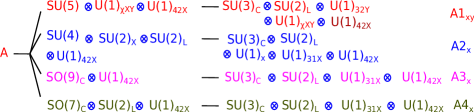
Figure 3: $E_{6}\rightarrow SO(10)\otimes U(1)_{42X}$ chains of subgroups, where $X,Y=R,I,A$ and $X\neq Y$.

Taking as inputs the values of the fine-structure constant and the corresponding quantities for the strong and weak interactions, we find the strength couplings at low energies by using the one-loop RGE equations [2]; however, we always find that for the $A1_{XY}$ chains of subgroups it is not possible to get the right order between the unification scales. That problem is related to the wrong prediction of the Weinberg angle in $SU(5)$. Although it is not possible to have a consistent picture for the embeddings $SU(5)\otimes U(1)\subset SO(10)\otimes U(1)\subset E_{6}$, there are solutions in most of the remaining $E_{6}$ breaking patterns.

4.1.1 $SU(4)\otimes SU(2)_{L}\otimes SU(2)\otimes U(1)\subset SO(10)\otimes U(1)\subset E_{6}$

From the three chains of subgroups $A2_{X}$ in figure (3) we can get low-energy $E_{6}$ models (LEE6Ms) i.e., models where at least one of the neutral currents in Eq. (9) does not contribute to the hypercharge, therefore, the corresponding vector boson is not necessary to have a consistent model. Usually, the fermion content of these models is smaller than the fundamental representation of $E_{6}$.

The $A2_{R}/U(1)_{42R}$ chain  is the Pati-Salam model [41, 47] (see figure (3)). The EW charges of this model are the same as those of $B2_{R}/U_{42R}$ (see figure (4)) and $C3_{R}/U_{42R}$ (see figure (5)) and are the same as the Left-Right (LR) symmetric model. The $A2_{A}/U_{42A}$ chain of subgroups corresponds to the alternative left-right model $Z_{ALR}$ [4]. The EW charges for this model were reported in [13] and are identical to those of $B2_{A}/U_{42A}$ and $C3_{A}/U_{42A}$. $A2_{I}$ is a new model in the literature even though is closely related to the second alternative model obtained from trinification [13]; the difference lies in the Abelian factor $U_{42I}$ (in [13] $Y$ is a linear combination of $U_{31I}$ and $U(1)_{I}$, while in the $SO(10)$ embedding $U_{42I}$ is in place of $U_{I}$). Identical EW charges are obtained from $B2_{I}$ and $C3_{I}$. Note that the coefficients of the hypercharge in $A3_{I}$ and $A4_{I}$ are identical to those of $A2_{I}$; however, due to the absence of the $U(1)_{I}$ factor in the chain of subgroups, in Eq. (12) there is no mixing with the corresponding vector boson $Z_{I}$. In $E_{6}$ the parameter space for every $Z^{\prime}$ of the $A2_{X}$ chain coincides with those of $C3_{X}$ in figure 6.

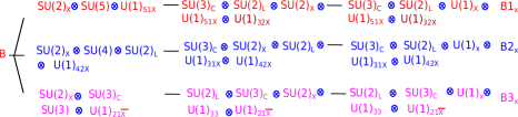
Figure 4: $E_{6}\rightarrow SU(2)_{X}\otimes SU(6)$ chains of subgroups, where $X=R,I,A$.

4.2 $SU(2)\otimes SU(6)\subset E_{6}$

The third chain of subgroups in which the SM hypercharge $U(1)_{Y}$ appears in a natural way is the $B1_{I}$ in figure (4). This model occurs in Calabi-Yau compactifications in string theory [3] and is commonly denoted as $Z_{\eta}$. The charges of this model correspond to those of $U(1)_{51I}$ (see Table D). In this chain of subgroups the $SU(5)$ is the same as that of Georgi-Glashow; however, the $U(1)_{51}$ factor is different from the corresponding factor in the embedding through $SO(10)$. The other two chains in $SU(2)_{X}\otimes SU(6)$ are $B2_{X}$ and $B3_{X}$. For these chains, the $Z^{\prime}$ charges of the LEE6Ms correspond to those of the Pati-Salam and trinification models, and their corresponding alternative versions, which have been studied in the previous section and in reference [13]. New models appear in the chains of subgroups containing $SU(2)_{L}\otimes SU(6)$; of particular interest are $C2_{X}$, which contain a $SU(5)$ different from the Georgi-Glashow one. This new $SU(5)$ allows a solution for the mass scales in $E_{6}$ from the one-loop RGE [2] (we saw above that such a solution is not possible either in the Georgi-Glashow model or its alternative versions). The same is true for the $C1_{xy}$ chains of subgroups. The chains $C3_{X}/U(1)_{42X}$ and $C4_{X}$ have the same $Z^{\prime}$ charges as the Pati-Salam and trinification models, respectively. The low-energy $Z^{\prime}$ charges for $C1_{X}$, $C2_{X}$ and $C3_{X}$ as a function of the $\theta$ mixing angle (see Eq. (12)) are shown in the Sanson-Flamsteed projection in figure (6).

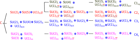
Figure 5: $E_{6}\rightarrow SU(2)_{L}\otimes SU(6)$ chains of subgroups, where $X,Y=R,I,A$ and $X\neq Y$.

4.3 $SU(3)\otimes SU(3)\otimes SU(3)$

The $SU(3)\otimes SU(3)\otimes SU(3)$ is the gauge group of trinification [48, 23, 49, 50, 51]. In table D are shown the three possible chains of breakings for this group. As was shown in reference [13], the charges of the three chains reduce to those of the universal 331 vector boson $Z_{331G}$  (see table 6 for the LHC constraints). A detailed study of these models and their EW constraints was presented in reference [13].

5 Low-energy models without unification.

The most general charges of any $E_{6}$-motivated $Z^{\prime}$ model is generated by the linear combination of three independent sets of charges associated with the $U(1)_{\kappa}$ symmetries, where $\kappa=a,b,c$. In appendix C, we showed that for unification models the values of $\alpha$ and $\beta$ corresponds to the vertical line which passes through $Z_{\psi}$ and $Z_{\chi}$. At low energies the parameter space of these models keeps close to this line, as can be seen in figure (6).

Without the unification hypothesis it is not possible to determine the preferred region in the parameter space. There are several models based on $E_{6}$ subgroups, and in some of them unification is not necessary to get a predictable model. In most of the well-known cases, the subgroup rank is less than the $E_{6}$ rank and at least one of the vector currents does not contribute to the electric charge. In order to ignore this current we set $\theta=0$ in Eq. (12), in such a way that for a fixed value of the couplings the $Z^{\prime}$ charges reduce to a single point in the Sanson-Flamsteed projection. Since the values of the couplings is arbitrary, by varying them we generate the parameter space for these models.

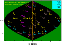
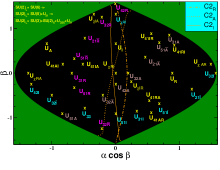
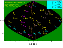
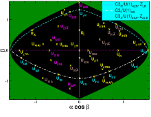
Figure 6: Sanson-Flamsteed projection of the $\alpha$-$\beta$ parameter space in $E_{6}$. The vertical line $\cos\beta=0$ represent the models with charges orthogonal to the SM hypercharge, thus, deviations of this line show that at low energies there is a mixing between the $Z^{\prime}$ and the field associated with the SM hypercharge. To obtain the values of $\alpha$ and $\beta$ in the top figures and in the bottom-left one we used the RGE [2] in order to get the $g_{a}$, $g_{b}$ and $g_{c}$ coupling strengths at the EW scale (from their initial values at the grand unification scale), then, we solved Eq. (C) varying $\theta$ between $-\pi$ and $\pi$. For the bottom-right figure, we put aside the unification hypothesis and, by ignoring the mixing with the fields associated with the charges that do not contribute to the electric charge, we explored the possible values for the coupling strengths; see section 5 for additional details.

For these models the hypercharge is the combination of the charges of two $U(1)^{\prime}\text{s}$. If we put $k_{c}=0$ and $\sin\theta=0$, the charges in Eq. (12) reduce to

$$g_{Z^{\prime}}\epsilon^{Z^{\prime}}_{L,R}= g_{Y}\left(k_{a}\frac{\epsilon^{b}_{L,R}}{\hat{\beta}}-\hat{\beta}k_{b}\epsilon^{a}_{L,R}\right)\ .$$ (28)

Owing to the fact that $Q_{c}$ does not contribute to the electric charge, in these models is possible to have a low-energy theory without the corresponding $Z^{\prime\prime}$ associated with $U(1)_{c}$. In section 4 we denoted them as LEE6Ms. In $E_{6}$ there are three chains of subgroups where one of the $Q_{k}$ corresponds to the SM hypercharge, in these cases, the SM is the LEE6M and, in principle, it does not require from other vector bosons to be a consistent theory. In Eq. (28) the $U_{a}$ and $U_{b}$ charges appear in a symmetric way, except by a global sign which, in general, can not be determined from the symmetry group.

In panel (6) the bottom-right figure shows the parameter space of some models based on $E_{6}$ subgroups. The horizontal dotted magenta line corresponds to the parameter space of the well-known LR models, which are LEE6Ms in the chains of subgroups $A2_{R}$, $B2_{R}$ and the $C3_{R}$. As expected, in this line appears the charges of the $Z_{B-L}$ ($U_{31R}$) and $Z_{R}$ ($U_{R}$). This line also represents the set of possible $Z^{\prime}$ models for flipped $SU(5)$ which are a linear combination of the $U_{\chi RA}$ and $U_{32A}$. The dashed cyan line contains the $Z^{\prime}$ parameter space of the alternative left-right model $Z_{ALR}$. These models are the linear combination of $U_{31A}$ and $U_{A}$ (the downphobic model $Z_{\not{d}}$). This line also corresponds to the possible $Z^{\prime}$ of the LEE6M of the chain of subgroups $A1_{AR}$ which has not been reported in the literature, as far as we know. The dot-dashed gray line is the set of the possible $Z^{\prime}$ models of the LEE6M associated with the chain of subgroups $C4_{I}$ which contains the universal 331 model [46, 40, 13]. We obtain these models from the linear combination of the $U(1)_{33}$ and the $U_{21\bar{I}}$, which have the quantum numbers of $\lambda_{8L}$ and $U(1)^{\prime}$ in the 331 models, respectively. This line is also generated from the third alternative left right model [13] and results from the linear combination of $U_{31I}$ (the leptophobic model $Z_{\not{L}}$) and $U_{42I}$. This line also corresponds to the possible $Z^{\prime}$ for the LEE6M of $C2_{I}$, which, to the best of our knowledge, has not been reported in the literature. This set of points contains the $Z_{\eta}$ ($U_{51I}$) model.

6 LHC constraints

Finally, we also report the most recent constraints from colliders and low-energy experiments on the neutral current parameters for some $Z^{\prime}$-motivated $E_{6}$ models and the sequential standard model (SSM). For the time being, the strongest constraints come from the proton-proton collisions data collected by the ATLAS experiment at the LHC with an integrated luminosities of 36.1 fb^-1 and 13.3 fb^-1 at a center of mass energy of 13 TeV [52, 53]. In particular, we used the upper limits at 95% C.L. on the total cross-section of the $Z^{\prime}$ decaying into dileptons (i.e., $e^{+}e^{-}$ and $\mu^{+}\mu^{-}$). Figure (7) shows the contours of the lower limits on the $M_{Z^{\prime}}$ at 95% C.L. We obtain these limits from the intersection of $\sigma^{\text{NLO}}(pp\rightarrow Z^{\prime}\rightarrow l^{-}l^{+})$ with the ATLAS 95% C.L. upper limits on the cross-section (for additional details see reference [21]). As a cross-check we calculated these limits for some models as shown in table 6 for various $E_{6}$-motivated $Z^{\prime}$ models and the SSM model. In order to compare, we also show in this figure the constraints for all the models reported by ATLAS. For the 36.1 fb^-1 data we multiply the theoretical cross-section by a global $K$ factor to reproduce the ATLAS constraints for the $Z_{\chi}$ model. This procedure was not necessary for the 13.3 fb^-1 dataset.

95$\%$ C.L. lower mass limits (in TeV) for $E_{6}$-motivated $Z^{\prime}$ models and the sequential standard model $Z_{\text{ssm}}$. These constraints come from the 36.1 fb^-1 and 13.3 fb^-1 datasets for proton-proton collision at a center of mass energy of $\sqrt{s}=13$ TeV [52, 53]. $Z^{\prime}$ model luminosity $Z_{\chi}$ $Z_{\psi}$ $Z_{\eta}$ $Z_{LR}$ $Z_{R}$ $Z_{N}$ $Z_{S}$ $Z_{I}$ $Z_{B-L}$ $Z_{\not{d}}$ $Z_{331G}$ $Z_{SSM}$ $M_{Z^{\prime}}$(^†fitted) (36.1fb^-1) 4.1^† 3.81 3.91 4.28 4.41 3.84 4.02 3.94 4.44 4.66 4.608 4.58 ATLAS (36.1fb^-1) 4.1 3.8 3.9 — — 3.8 4.0 4.0 — — — 4.5 $M_{Z^{\prime}}$ (13.3fb^-1) 3.62 3.35 3.43 3.77 3.92 3.38 3.54 3.47 3.95 4.15 4.10 4.05 ATLAS (13.3fb^-1) 3.66 3.36 3.43 — — 3.41 3.62 3.55 — — — 4.05

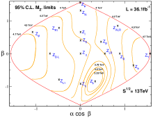
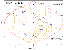
Figure 7: $\alpha$-$\beta$ Sanson-Flamsteed projection of the $Z^{\prime}$ parameter space in $E_{6}$. The contours show the 95% C.L. lower limits on the $Z^{\prime}$ mass (in TeV).

7 Conclusions

In the present work we have reported the most general expression for the chiral charges of a neutral gauge boson $Z^{\prime}$ coming from an $E_{6}$ unification model, in terms of the EW parameters and the charges of the $U(1)$ factors in the chain of subgroups.

We also showed for any breaking pattern that, the charges of SM hypercharge are orthogonal to the corresponding charges of the $Z^{\prime}$ gauge boson i.e., $\sum_{f\in 27}Y(f)Q_{Z^{\prime}}(f)=0$ (see section 3), if the values of the $g_{\kappa}$ coupling strengths associated with the $U(1)_{\kappa}$ factors of the chains of breakings are equal to each other. Due to the RGE the couplings are no longer identical at low energies, therefore there must be a mixing between the field associated with $Y$ and the $Z^{\prime}$. This mixing can modify several observables as it has been shown in reference [31, 33, 20].

Pure neutral gauge bosons coming from $E_{6}$ are $Z_{\psi}$ and $Z_{\chi}$ as introduced in section 4.1 but the physical neutral states $Z^{\prime}$ and $Z^{\prime\prime}$ are a mixing of those states according to Eqs. (26) and (27), which define the $\alpha$ and $\beta$ angles in our analysis. By using the RGE [2] and assuming $E_{6}$ unification, we showed that for most of the chains of breaking in $E_{6}$ it is possible to solve the equations for the mass scales in a consistent way (one important exception are the chains of subgroups that contain the Georgi-Glashow $SU(5)$ model and their alternative versions). This procedure allowed us to calculate the low-energy coupling strengths for several chains of subgroups and the $Z^{\prime}$ parameter space in the Sanson-Flamsteed projection. It is worth noting that in $E_{6}$ unification at low energies the parameter space of these models keeps close to the mentioned vertical line as can be seen in figure (6). To the best of our knowledge, several of the analyzed chains of subgroups presented here are new in the literature.

The most general charges of any $E_{6}$-motivated $Z^{\prime}$ model is generated by the linear combination of three independent set of charges associated with the different $U(1)$ symmetries. By putting aside the unification hypothesis it is not possible to determine the preferred region in the parameter space; however, by ignoring the mixing with the associated charges that do not contribute to the electric charge, the corresponding parameter space reduces to a single line in the $\alpha$-$\beta$ Sanson-Flamsteed projection as shown for some models in the bottom right figure in (6).

By using the most recent upper limits on the cross-section for extra gauge vector bosons $Z^{\prime}$ decaying into dileptons form ATLAS data at 13 TeV with accumulated luminosities of 36.1fb^-1 [52] and 13.3fb^-1 [53] for the Drell-Yang processes $pp\rightarrow Z(\gamma)\rightarrow l^{+}l^{-}$, we set 95$\%$ C.L. lower limits on the $Z^{\prime}$ mass for the typical $E_{6}$ benchmark models. We also reported the contours in the 95% C.L. $Z^{\prime}$ mass limits for the entire $Z^{\prime}$ parameter space in $E_{6}$. Our results are in agreement with the lower mass limits reported by ATLAS for the $E_{6}$-motivated $Z^{\prime}$ models and the sequential standard model $Z_{\text{SSM}}$.

Finally it is important to stress that the recent LHCb anomalies could also be explained by $E_{6}$ subgroups [54, 55, 56, 57, 58, 59]. A natural continuation of our work would be to find which of these models are able to explain the anomalies. That is an interesting question since the $E_{6}$ models, in general, have been considered as phenomenologically safe.

Appendix A Rotation matrix

Let us now consider an explicit representation for the orthogonal matrix $\mathcal{O}$ in terms of three angles $\omega$, $\phi$ and $\theta$, which are allowed to take values in the $[-\pi,\pi)$ interval. For convenience we choose

$$\mathcal{O} =\begin{pmatrix}1&0&0&0\\ 0&\cos\omega&-\sin\omega&0\\ 0&\sin\omega&\cos\omega&0\\ 0&0&0&1\end{pmatrix}\begin{pmatrix}1&0&0&0\\ 0&\cos\phi&0&-\sin\phi\\ 0&0&1&0\\ 0&\sin\phi&0&\cos\phi\end{pmatrix}\begin{pmatrix}1&0&0&0\\ 0&1&0&0\\ 0&0&\cos\theta&-\sin\theta\\ 0&0&\sin\theta&\cos\theta\end{pmatrix}\ .$$

Relations in Eq.(10) imply then that

$$\cos\phi\cos\omega=\frac{k_{a}g_{Y}}{g_{a}}\ ,\hskip 14.22636pt\cos\phi\sin\omega=\frac{k_{b}g_{Y}}{g_{b}}\ ,\hskip 14.22636pt\sin\phi=\frac{k_{c}g_{Y}}{g_{c}}\ ,$$ (29)

which allows us to write the $\phi$ and $\omega$ angles in terms of the $g_{a}$ and $g_{b}$ coupling constants and of the $k_{a}$, $k_{b}$ and $k_{c}$ coefficients. The $\theta$ angle, however, cannot be fixed and must be considered to be another free-parameter. It is easy to show that

$$\cos\phi =\hat{\alpha}_{c}\frac{g_{Y}}{g_{c}},$$ (30)

$$\cos\omega =\frac{k_{a}g_{c}}{\hat{\alpha}_{c}g_{a}}\ ,$$ (31)

$$\sin\omega =\frac{k_{b}g_{c}}{\hat{\alpha}_{c}g_{b}}\ ,$$ (32)

where

$$\hat{\alpha}_{c}=g_{c}\sqrt{\frac{k_{a}^{2}}{g_{a}^{2}}+\frac{k_{b}^{2}}{g_{b}^{2}}}=\sqrt{\frac{g_{c}^{2}}{g^{2}}\cot^{2}\theta_{W}-k_{c}^{2}}\ .$$ (33)

Appendix B $Z^{\prime}$ charges

From the Lagrangian

$$-\mathcal{L}_{NC}= gJ_{3L}^{\mu}A_{3L\mu}+g_{a}J_{a\mu}A^{\mu}_{a}+g_{b}J_{b\mu}A^{\mu}_{b}+g_{c}J_{c\mu}A^{\mu}_{c}$$

$$= g_{\kappa}J_{\kappa\mu}A^{\mu}_{\kappa}=g_{\kappa^{\prime\prime}}J_{\kappa^{\prime\prime}\mu}\mathcal{O}_{\kappa^{\prime\prime}\kappa^{\prime}}\mathcal{O}_{\kappa^{\prime}\kappa}^{T}A^{\mu}_{\kappa}$$

$$\equiv g_{\kappa^{\prime}}J_{\kappa^{\prime}\mu}Z_{\kappa^{\prime}}^{\mu}\ ,$$ (34)

where $\kappa$ runs over $3L,a,b,c$ and $k^{\prime}$ and $k^{\prime\prime}$ runs over $3L,Y,Z^{\prime},Z^{\prime\prime}$, from this equation we obtain

$$J_{\kappa^{\prime}\mu}=J_{\kappa\mu}\mathcal{O}_{\kappa\kappa^{\prime}}=\mathcal{O}_{\kappa^{\prime}\kappa}^{T}J_{\kappa\mu}\ .$$ (35)

From this equation the current associated with the $Z^{\prime}$ is given by

$$g_{Z^{\prime}}J_{Z^{\prime}}= g_{Y}\left(-\frac{k_{a}J_{a}^{\mu}+k_{b}J_{b}^{\mu}}{\hat{\alpha}_{c}}k_{c}+\hat{\alpha}_{c}J_{c}^{\mu}\right)\sin\theta+\frac{g_{c}}{\hat{\alpha}_{c}}\left(\frac{k_{a}J_{b}^{\mu}}{\hat{\beta}}-\hat{\beta}k_{b}J_{a}^{\mu}\right)\cos\theta\ ,$$ (36)

$$g_{Z^{\prime\prime}}J_{Z^{\prime\prime}}= g_{Y}\left(-\frac{k_{a}J_{a}^{\mu}+k_{b}J_{b}^{\mu}}{\hat{\alpha}_{c}}k_{c}+\hat{\alpha}_{c}J_{c}^{\mu}\right)\cos\theta-\frac{g_{c}}{\hat{\alpha}_{c}}\left(\frac{k_{a}J_{b}^{\mu}}{\hat{\beta}}-\hat{\beta}k_{b}J_{a}^{\mu}\right)\sin\theta\ ,$$ (37)

where $\hat{\beta}=\frac{g_{a}}{g_{b}}$. For the LEE6Ms ($c=0$ and $\sin\theta=0$) we obtain

$$g_{Z^{\prime}}J_{g_{Z^{\prime}}}^{\mu}= g_{Y}\left(k_{a}\frac{J_{b}^{\mu}}{\hat{\beta}}-\hat{\beta}k_{b}J_{a}^{\mu}\right)=g_{Y}\left(k_{b}\frac{J_{b}^{\mu}}{\hat{\alpha}_{a}}k_{a}-\hat{\alpha}_{a}J_{a}^{\mu}\right)\text{sign}(k_{b})\ ,$$ (38)

$$= g_{Y}\left(\hat{\alpha}_{b}J_{b}^{\mu}-k_{a}\frac{J_{a}^{\mu}}{\hat{\alpha}_{b}}k_{b}\right)\text{sign}(k_{a})\ ,$$ (39)

where

$$\hat{\alpha}_{a,b}=\sqrt{\frac{g_{a,b}^{2}}{g^{2}}\cot^{2}\theta_{W}-k_{a,b}^{2}}\ .$$ (40)

Appendix C Sanson-Flamsteed Projection

As we mentioned in section 4 in general any $Z^{\prime}$ in $E_{6}$ can be written as a linear combination of three linear independent models. One usual basis is given by

$$g_{Z^{\prime}}\epsilon^{Z^{\prime}}_{L,R}= g_{Z^{\prime}}\left(\cos\alpha\cos\beta\epsilon^{Z_{\chi}}_{L,R}+\sin\alpha\cos\beta Y_{L,R}+\sin\beta\epsilon^{Z_{\psi}}_{L,R}\right)\eta\ ,$$

$$= A_{L,R}\sin\theta+B_{L,R}\cos\theta\ ,\hskip 5.69046pt\text{with}\hskip 5.69046pt\eta=\pm 1\ ,$$ (41)

where the $\epsilon^{Z_{\chi}}_{L,R}$ and $\epsilon^{Z_{\psi}}_{L,R}$ are the chiral charges of the $Z_{\chi}$ and $Z_{\psi}$ models, respectively. In this equation $g_{Z^{\prime}}$ is given by the Eq. 16. In the last line we equate the chiral charges for the $Z^{\prime}$ associated to a given chain of subgroups Eq. (12) to the general expression of the $E_{6}$ motivated $Z^{\prime}$ charges in the $\alpha\text{-}\beta$ parameter space Eq. 27. We can obtain the partial unification mass scales for every breaking pattern according to the reference [2]. By evolving $g_{a}$, $g_{b}$ and $g_{c}$ down to low energies for every $\theta$ there is a pair $(\alpha,\beta)$ according with the equation (C). $\theta$ parametrizes the mixing between the $Z^{\prime}$ and $Z^{\prime\prime}$ the charges (C) and the corresponding parameter space to low energies is shown in figure (6). It is important to notice that at low energies the charges keep close to the vertical line which corresponds to the unification parameter space.

Appendix D tables

$E_{6}$ normalized chiral charges of ordinary fermions and right-handed neutrinos. Here $l_{L}=(\nu_{L},e_{L})^{T}$ and $q_{L}=(u_{L},d_{L})^{T}$ denote the left-handed lepton and quark doublets. Model $\epsilon_{L}(l)$ $\epsilon_{R}(\nu)$ $\epsilon_{R}(e)$ $\epsilon_{L}(q)$ $\epsilon_{R}(u)$ $\epsilon(d)$ $U_{Y}$ $-\frac{1}{2}\sqrt{\frac{3}{5}}$ $0$ $-\sqrt{\frac{3}{5}}$ $\frac{1}{2\sqrt{15}}$ $\frac{2}{\sqrt{15}}$ $-\frac{1}{\sqrt{15}}$ $U_{R}$ $0$ $\frac{1}{2}$ $-\frac{1}{2}$ $0$ $\frac{1}{2}$ $-\frac{1}{2}$ $U_{I}$ $\frac{1}{2}$ $\frac{1}{2}$ $0$ $0$ $0$ $-\frac{1}{2}$ $U_{A}$ $\frac{1}{2}$ $0$ $\frac{1}{2}$ $0$ $-\frac{1}{2}$ $0$ $U_{33}$ $\frac{1}{2\sqrt{3}}$ $\frac{1}{\sqrt{3}}$ $\frac{1}{\sqrt{3}}$ $-\frac{1}{2\sqrt{3}}$ $0$ $0$ $U_{21\overline{R}}$ $\frac{1}{\sqrt{3}}$ $\frac{1}{2\sqrt{3}}$ $\frac{1}{2\sqrt{3}}$ $0$ $-\frac{1}{2\sqrt{3}}$ $-\frac{1}{2\sqrt{3}}$ $U_{21\overline{I}}$ $-\frac{1}{2\sqrt{3}}$ $\frac{1}{2\sqrt{3}}$ $-\frac{1}{\sqrt{3}}$ $0$ $\frac{1}{\sqrt{3}}$ $-\frac{1}{2\sqrt{3}}$ $U_{21\overline{A}}$ $\frac{1}{2\sqrt{3}}$ $\frac{1}{\sqrt{3}}$ $-\frac{1}{2\sqrt{3}}$ $0$ $\frac{1}{2\sqrt{3}}$ $-\frac{1}{\sqrt{3}}$ $U_{31R}$ $\frac{1}{2}\sqrt{\frac{3}{2}}$ $\frac{1}{2}\sqrt{\frac{3}{2}}$ $\frac{1}{2}\sqrt{\frac{3}{2}}$ $-\frac{1}{2\sqrt{6}}$ $-\frac{1}{2\sqrt{6}}$ $-\frac{1}{2\sqrt{6}}$ $U_{31I}$ $0$ $\frac{1}{2}\sqrt{\frac{3}{2}}$ $0$ $-\frac{1}{2\sqrt{6}}$ $\frac{1}{\sqrt{6}}$ $-\frac{1}{2\sqrt{6}}$ $U_{31A}$ $0$ $0$ $-\frac{1}{2}\sqrt{\frac{3}{2}}$ $\frac{1}{2\sqrt{6}}$ $\frac{1}{2\sqrt{6}}$ $-\frac{1}{\sqrt{6}}$ $U_{42R}$ $\frac{1}{2\sqrt{6}}$ $-\frac{1}{2\sqrt{6}}$ $-\frac{1}{2\sqrt{6}}$ $\frac{1}{2\sqrt{6}}$ $-\frac{1}{2\sqrt{6}}$ $-\frac{1}{2\sqrt{6}}$ $U_{42I}$ $\frac{1}{\sqrt{6}}$ $\frac{1}{2\sqrt{6}}$ $\sqrt{\frac{2}{3}}$ $-\frac{1}{2\sqrt{6}}$ $-\frac{1}{\sqrt{6}}$ $\frac{1}{2\sqrt{6}}$ $U_{42A}$ $\frac{1}{\sqrt{6}}$ $\sqrt{\frac{2}{3}}$ $\frac{1}{2\sqrt{6}}$ $-\frac{1}{2\sqrt{6}}$ $\frac{1}{2\sqrt{6}}$ $-\frac{1}{\sqrt{6}}$ $U_{32R}$ $\frac{1}{2}\sqrt{\frac{3}{5}}$ $0$ $0$ $\frac{1}{2\sqrt{15}}$ $-\frac{1}{\sqrt{15}}$ $-\frac{1}{\sqrt{15}}$ $U_{32I}$ $-\frac{1}{2}\sqrt{\frac{3}{5}}$ $0$ $-\sqrt{\frac{3}{5}}$ $\frac{1}{2\sqrt{15}}$ $\frac{2}{\sqrt{15}}$ $-\frac{1}{\sqrt{15}}$ $U_{32A}$ $\frac{1}{2}\sqrt{\frac{3}{5}}$ $\sqrt{\frac{3}{5}}$ $0$ $-\frac{1}{2\sqrt{15}}$ $\frac{1}{\sqrt{15}}$ $-\frac{2}{\sqrt{15}}$ $U_{32\overline{R}}$ $0$ $\frac{1}{2}\sqrt{\frac{3}{5}}$ $\frac{1}{2}\sqrt{\frac{3}{5}}$ $-\frac{1}{\sqrt{15}}$ $\frac{1}{2\sqrt{15}}$ $\frac{1}{2\sqrt{15}}$ $U_{32\overline{I}}$ $\frac{1}{2}\sqrt{\frac{3}{5}}$ $\frac{1}{2}\sqrt{\frac{3}{5}}$ $\sqrt{\frac{3}{5}}$ $-\frac{1}{\sqrt{15}}$ $-\frac{1}{\sqrt{15}}$ $\frac{1}{2\sqrt{15}}$ $U_{32\overline{A}}$ $\frac{1}{2}\sqrt{\frac{3}{5}}$ $\sqrt{\frac{3}{5}}$ $\frac{1}{2}\sqrt{\frac{3}{5}}$ $-\frac{1}{\sqrt{15}}$ $\frac{1}{2\sqrt{15}}$ $-\frac{1}{\sqrt{15}}$ $U_{51R}$ $\frac{2}{\sqrt{15}}$ $\frac{1}{2}\sqrt{\frac{5}{3}}$ $\frac{1}{2}\sqrt{\frac{5}{3}}$ $-\frac{1}{\sqrt{15}}$ $-\frac{1}{2\sqrt{15}}$ $-\frac{1}{2\sqrt{15}}$ $U_{51I}$ $\frac{1}{2\sqrt{15}}$ $\frac{1}{2}\sqrt{\frac{5}{3}}$ $\frac{1}{\sqrt{15}}$ $-\frac{1}{\sqrt{15}}$ $\frac{1}{\sqrt{15}}$ $-\frac{1}{2\sqrt{15}}$ $U_{51A}$ $\frac{1}{2\sqrt{15}}$ $\frac{1}{\sqrt{15}}$ $\frac{1}{2}\sqrt{\frac{5}{3}}$ $-\frac{1}{\sqrt{15}}$ $-\frac{1}{2\sqrt{15}}$ $\frac{1}{\sqrt{15}}$ $U_{51\overline{R}}$ $\frac{1}{2}\sqrt{\frac{5}{3}}$ $\frac{2}{\sqrt{15}}$ $\frac{2}{\sqrt{15}}$ $-\frac{1}{2\sqrt{15}}$ $-\frac{1}{\sqrt{15}}$ $-\frac{1}{\sqrt{15}}$ $U_{51\overline{I}}$ $-\frac{1}{2\sqrt{15}}$ $\frac{2}{\sqrt{15}}$ $-\frac{1}{\sqrt{15}}$ $-\frac{1}{2\sqrt{15}}$ $\frac{2}{\sqrt{15}}$ $-\frac{1}{\sqrt{15}}$ $U_{51\overline{A}}$ $\frac{1}{2\sqrt{15}}$ $\frac{1}{\sqrt{15}}$ $-\frac{2}{\sqrt{15}}$ $\frac{1}{2\sqrt{15}}$ $\frac{1}{\sqrt{15}}$ $-\frac{2}{\sqrt{15}}$ $U_{41IA}$ $\sqrt{\frac{2}{5}}$ $\sqrt{\frac{2}{5}}$ $\frac{3}{2\sqrt{10}}$ $-\frac{1}{2\sqrt{10}}$ $-\frac{1}{2\sqrt{10}}$ $-\frac{1}{\sqrt{10}}$ $U_{41AR}$ $-\frac{1}{2\sqrt{10}}$ $\frac{3}{2\sqrt{10}}$ $-\frac{1}{2\sqrt{10}}$ $-\frac{1}{2\sqrt{10}}$ $\frac{3}{2\sqrt{10}}$ $-\frac{1}{2\sqrt{10}}$ $U_{41RI}$ $0$ $\frac{1}{2\sqrt{10}}$ $-\sqrt{\frac{2}{5}}$ $\frac{1}{2\sqrt{10}}$ $\frac{1}{\sqrt{10}}$ $-\frac{3}{2\sqrt{10}}$ $U_{41AI}$ $\sqrt{\frac{2}{5}}$ $\frac{3}{2\sqrt{10}}$ $\sqrt{\frac{2}{5}}$ $-\frac{1}{2\sqrt{10}}$ $-\frac{1}{\sqrt{10}}$ $-\frac{1}{2\sqrt{10}}$ $U_{41RA}$ $0$ $\sqrt{\frac{2}{5}}$ $-\frac{1}{2\sqrt{10}}$ $-\frac{1}{2\sqrt{10}}$ $\frac{3}{2\sqrt{10}}$ $-\frac{1}{\sqrt{10}}$ $U_{41IR}$ $\frac{1}{2\sqrt{10}}$ $\frac{1}{2\sqrt{10}}$ $-\frac{3}{2\sqrt{10}}$ $\frac{1}{2\sqrt{10}}$ $\frac{1}{2\sqrt{10}}$ $-\frac{3}{2\sqrt{10}}$ $U_{\chi RI}$ $\frac{3}{2\sqrt{10}}$ $\frac{1}{2}\sqrt{\frac{5}{2}}$ $\frac{1}{2\sqrt{10}}$ $-\frac{1}{2\sqrt{10}}$ $\frac{1}{2\sqrt{10}}$ $-\frac{3}{2\sqrt{10}}$ $U_{\chi AR}$ $-\frac{1}{\sqrt{10}}$ $0$ $-\frac{1}{2}\sqrt{\frac{5}{2}}$ $\frac{1}{2\sqrt{10}}$ $\frac{3}{2\sqrt{10}}$ $-\frac{1}{\sqrt{10}}$ $U_{\chi IA}$ $\frac{1}{\sqrt{10}}$ $-\frac{1}{2\sqrt{10}}$ $0$ $\frac{1}{2\sqrt{10}}$ $-\frac{1}{\sqrt{10}}$ $-\frac{1}{2\sqrt{10}}$ $U_{\chi IR}$ $\frac{1}{\sqrt{10}}$ $\frac{1}{2}\sqrt{\frac{5}{2}}$ $0$ $-\frac{1}{2\sqrt{10}}$ $\frac{1}{\sqrt{10}}$ $-\frac{3}{2\sqrt{10}}$ $U_{\chi RA}$ $\frac{3}{2\sqrt{10}}$ $\frac{1}{2\sqrt{10}}$ $\frac{1}{2}\sqrt{\frac{5}{2}}$ $-\frac{1}{2\sqrt{10}}$ $-\frac{3}{2\sqrt{10}}$ $\frac{1}{2\sqrt{10}}$ $U_{\chi AI}$ $\frac{1}{\sqrt{10}}$ $0$ $-\frac{1}{2\sqrt{10}}$ $\frac{1}{2\sqrt{10}}$ $-\frac{1}{2\sqrt{10}}$ $-\frac{1}{\sqrt{10}}$

Models arising from the $E_{6}\longrightarrow SO(10)\otimes U(1)_{42X}\longrightarrow SU(3)_{C}\otimes SU(2)_{L}\otimes G\longrightarrow G_{SM}$ chains of subgroups, where $G_{SM}\equiv SU(3)_{C}\otimes SU(2)_{L}\otimes U(1)_{Y}$. Model $G$ factor $A1_{XY}$ $U(1)_{32Y}\otimes U(1)_{\chi XY}\otimes U(1)_{42X}$ $k_{a}$ $k_{b}$ $k_{c}$ $A1_{IR}$: $U(1)_{32R}\otimes U(1)_{\chi IR}\otimes U(1)_{42I}$ $-\frac{1}{\sqrt{15}}$ $\frac{1}{\sqrt{10}}$ $-\sqrt{\frac{3}{2}}$ $A1_{AR}$: $U(1)_{32R}\otimes U(1)_{\chi AR}\otimes U(1)_{42A}$ $-\frac{1}{\sqrt{15}}$ $2\sqrt{\frac{2}{5}}$ $0$ $A1_{RI}$: $U(1)_{32I}\otimes U(1)_{\chi RI}\otimes U(1)_{42R}$ $\sqrt{\frac{5}{3}}$ $0$ $0$  [36, 1, 24] $A1_{AI}$: $U(1)_{32I}\otimes U(1)_{\chi AI}\otimes U(1)_{42A}$ $\sqrt{\frac{5}{3}}$ $0$ $0$  [12] $A1_{RA}$: $U(1)_{32A}\otimes U(1)_{\chi RA}\otimes U(1)_{42R}$ $\frac{1}{\sqrt{15}}$ $-2\sqrt{\frac{2}{5}}$ $0$  [1] $A1_{IA}$: $U(1)_{32A}\otimes U(1)_{\chi IA}\otimes U(1)_{42I}$ $\frac{1}{\sqrt{15}}$ $-\frac{1}{\sqrt{10}}$ $-\sqrt{\frac{3}{2}}$ $A2_{X}$ $U(1)_{X}\otimes U(1)_{31X}\otimes U(1)_{42X}$ $k_{a}$ $k_{b}$ $k_{c}$ $A2_{R}$: $U(1)_{R}\otimes U(1)_{31R}\otimes U(1)_{42R}$ $1$ $-\sqrt{\frac{2}{3}}$ $0$  [41, 47] $A2_{I}$: $U(1)_{I}\otimes U(1)_{31I}\otimes U(1)_{42I}$ $0$ $\frac{1}{\sqrt{6}}$ $-\sqrt{\frac{3}{2}}$  [13] $A2_{A}$: $U(1)_{A}\otimes U(1)_{31A}\otimes U(1)_{42A}$ $-1$ $\sqrt{\frac{2}{3}}$ $0$  [4] $A3_{X}$ $U(1)_{31X}\otimes U(1)_{42X}$ $k_{a}$ $k_{b}$ $A3_{R}$: $U(1)_{31R}\otimes U(1)_{42R}$ $--$ $--$ $A3_{I}$: $U(1)_{31I}\otimes U(1)_{42I}$ $\frac{1}{\sqrt{6}}$ $-\sqrt{3/2}$ $A3_{A}$: $U(1)_{31A}\otimes U(1)_{42A}$ $--$ $--$

Models arising from the $E_{6}\longrightarrow SU(2)_{X}\otimes SU(6)\longrightarrow SU(3)_{C}\otimes SU(2)_{L}\otimes G\longrightarrow G_{SM}$ chains of subgroups, where $G_{SM}\equiv SU(3)_{C}\otimes SU(2)_{L}\otimes U(1)_{Y}$. Model $G$ factor $B1_{X}$ $U(1)_{32X}\otimes U(1)_{51X}\otimes U(1)_{X}$ $k_{a}$ $k_{b}$ $k_{c}$ $B1_{R}$: $U(1)_{32R}\otimes U(1)_{51R}\otimes U(1)_{R}$ $-\frac{1}{\sqrt{15}}$ $-\sqrt{\frac{3}{5}}$ $1$ $B1_{I}$: $U(1)_{32I}\otimes U(1)_{51I}\otimes U(1)_{I}$ $\sqrt{\frac{5}{3}}$ $0$ $0$  [3] $B1_{A}$: $U(1)_{32A}\otimes U(1)_{51A}\otimes U(1)_{A}$ $\frac{1}{\sqrt{15}}$ $-\sqrt{\frac{3}{5}}$ $-1$ $B2_{X}$ $U(1)_{31X}\otimes U(1)_{42X}\otimes U(1)_{X}$     same as $A2_{X}$ $B3_{X}$ $U(1)_{33}\otimes U(1)_{21\overline{X}}\otimes U(1)_{X}$     same as $D_{X}$

Models arising from the $E_{6}\longrightarrow SU(2)_{L}\otimes SU(6)\longrightarrow SU(3)_{C}\otimes SU(2)_{L}\otimes G\longrightarrow G_{SM}$ chains of subgroups, where $G_{SM}\equiv SU(3)_{C}\otimes SU(2)_{L}\otimes U(1)_{Y}$. Model $G$ factor $C1_{XY}$ $U(1)_{31Y}\otimes U(1)_{41XY}\otimes U(1)_{51\overline{X}}$ $k_{a}$ $k_{b}$ $k_{c}$ $C1_{IR}$: $U(1)_{31R}\otimes U(1)_{41IR}\otimes U(1)_{51\overline{I}}$ $-\sqrt{\frac{2}{3}}$ $\sqrt{\frac{2}{5}}$ $\sqrt{\frac{3}{5}}$ $C1_{AR}$: $U(1)_{31R}\otimes U(1)_{41AR}\otimes U(1)_{51\overline{A}}$ $-\sqrt{\frac{2}{3}}$ $\sqrt{\frac{2}{5}}$ $\sqrt{\frac{3}{5}}$ $C1_{RI}$: $U(1)_{31I}\otimes U(1)_{41RI}\otimes U(1)_{51\overline{R}}$ $\frac{1}{\sqrt{6}}$ $\frac{3}{\sqrt{10}}$ $-\sqrt{\frac{3}{5}}$ $C1_{AI}$: $U(1)_{31I}\otimes U(1)_{41AI}\otimes U(1)_{51\overline{A}}$ $\frac{1}{\sqrt{6}}$ $-\frac{3}{\sqrt{10}}$ $\sqrt{\frac{3}{5}}$ $C1_{RA}$: $U(1)_{31A}\otimes U(1)_{41RA}\otimes U(1)_{51\overline{R}}$ $\sqrt{\frac{2}{3}}$ $\sqrt{\frac{2}{5}}$ $-\sqrt{\frac{3}{5}}$ $C1_{IA}$: $U(1)_{31A}\otimes U(1)_{41IA}\otimes U(1)_{51\overline{I}}$ $\sqrt{\frac{2}{3}}$ $-\sqrt{\frac{2}{5}}$ $\sqrt{\frac{3}{5}}$ $C2_{X}$ $U(1)_{X}\otimes U(1)_{32\overline{X}}\otimes U(1)_{51\overline{X}}$ $k_{a}$ $k_{b}$ $k_{c}$ $C2_{R}$: $U(1)_{R}\otimes U(1)_{32\overline{R}}\otimes U(1)_{51\overline{R}}$ $1$ $-\frac{1}{\sqrt{15}}$ $-\sqrt{\frac{3}{5}}$ $C2_{I}$: $U(1)_{I}\otimes U(1)_{32\overline{I}}\otimes U(1)_{51\overline{I}}$ $0$ $-\frac{4}{\sqrt{15}}$ $\sqrt{\frac{3}{5}}$ $C2_{A}$: $U(1)_{A}\otimes U(1)_{32\overline{A}}\otimes U(1)_{51\overline{A}}$ $-1$ $-\frac{1}{\sqrt{15}}$ $\sqrt{\frac{3}{5}}$ $C3_{X}$ $U(1)_{X}\otimes U(1)_{31X}\otimes U(1)_{42X}$     same as $A2_{X}$ $C4_{X}$ $U(1)_{X}\otimes U(1)_{21\overline{X}}\otimes U(1)_{33}$     same as $D_{X}$

Models arising from the $E_{6}\longrightarrow SU(3)\otimes SU(3)\otimes SU(3)\longrightarrow SU(3)_{C}\otimes SU(2)_{L}\otimes G\longrightarrow G_{SM}$ chains of subgroups, where $G_{SM}\equiv SU(3)_{C}\otimes SU(2)_{L}\otimes U(1)_{Y}$. Model $G$ factor $D_{X}$ $U(1)_{X}\otimes U(1)_{21\overline{X}}\otimes U(1)_{33}$ $k_{a}$ $k_{b}$ $k_{c}$ $D_{R}$: $U(1)_{R}\otimes U(1)_{21\overline{R}}\otimes U(1)_{33}$ $1$ $-\frac{1}{\sqrt{3}}$ $-\frac{1}{\sqrt{3}}$ $D_{I}$: $U(1)_{I}\otimes U(1)_{21\overline{I}}\otimes U(1)_{33}$ $0$ $\frac{2}{\sqrt{3}}$ $-\frac{1}{\sqrt{3}}$  [48, 23, 49, 50, 13] $D_{A}$: $U(1)_{A}\otimes U(1)_{21\overline{A}}\otimes U(1)_{33}$ $-1$ $\frac{1}{\sqrt{3}}$ $-\frac{1}{\sqrt{3}}$

References

- [1] S. M. Barr, Phys. Lett. 112B, 219 (1982), 10.1016/0370-2693(82)90966-2.
- [2] R. W. Robinett and J. L. Rosner, Phys. Rev. D26, 2396 (1982), 10.1103/PhysRevD.26.2396.
- [3] E. Witten, Nucl. Phys. B258, 75 (1985), 10.1016/0550-3213(85)90603-0.
- [4] E. Ma, Phys. Rev. D36, 274 (1987), 10.1103/PhysRevD.36.274.
- [5] E. Ma, Phys. Lett. B380, 286 (1996), arXiv:hep-ph/9507348 [hep-ph], 10.1016/0370-2693(96)00524-2.
- [6] R. Martinez, W. A. Ponce and L. A. Sanchez, Phys. Rev. D65, 055013 (2002), arXiv:hep-ph/0110246 [hep-ph], 10.1103/PhysRevD.65.055013.
- [7] E. Rojas and J. Erler, JHEP 10, 063 (2015), arXiv:1505.03208 [hep-ph], 10.1007/JHEP10(2015)063.
- [8] S. F. Mantilla, R. Martinez, F. Ochoa and C. F. Sierra, Nucl. Phys. B911, 338 (2016), arXiv:1602.05216 [hep-ph], 10.1016/j.nuclphysb.2016.08.014.
- [9] C.-S. Huang, W.-J. Li and X.-H. Wu (2017), arXiv:1705.01411 [hep-ph].
- [10] A. E. Cárcamo Hernández, S. Kovalenko, J. W. F. Valle and C. A. Vaquera-Araujo, JHEP 07, 118 (2017), arXiv:1705.06320 [hep-ph], 10.1007/JHEP07(2017)118.
- [11] J. P. Derendinger, J. E. Kim and D. V. Nanopoulos, Phys. Lett. 139B, 170 (1984), 10.1016/0370-2693(84)91238-3.
- [12] S. F. King, S. Moretti and R. Nevzorov, Phys. Rev. D73, 035009 (2006), arXiv:hep-ph/0510419 [hep-ph], 10.1103/PhysRevD.73.035009.
- [13] O. Rodríguez, R. H. Benavides, W. A. Ponce and E. Rojas, Phys. Rev. D95, 014009 (2017), arXiv:1605.00575 [hep-ph], 10.1103/PhysRevD.95.014009.
- [14] S. Dimopoulos and L. J. Hall, Nucl. Phys. B255, 633 (1985), 10.1016/0550-3213(85)90157-9.
- [15] J. Rizos and K. Tamvakis, Phys. Lett. B414, 277 (1997), arXiv:hep-ph/9702295 [hep-ph], 10.1016/S0370-2693(97)01181-7.
- [16] Q. Shafi and Z. Tavartkiladze, Nucl. Phys. B552, 67 (1999), arXiv:hep-ph/9807502 [hep-ph], 10.1016/S0550-3213(99)00178-9.
- [17] A. E. Faraggi, M. Paraskevas, J. Rizos and K. Tamvakis, Phys. Rev. D90, 015036 (2014), arXiv:1405.2274 [hep-ph], 10.1103/PhysRevD.90.015036.
- [18] P. V. Dong, D. T. Huong, F. S. Queiroz, J. W. F. Valle and C. A. Vaquera-Araujo (2017), arXiv:1710.06951 [hep-ph].
- [19] R. Benavides, L. A. Muñoz, W. A. Ponce, O. Rodríguez and E. Rojas, Phys. Rev. D95, 115018 (2017), arXiv:1612.07660 [hep-ph], 10.1103/PhysRevD.95.115018.
- [20] P. Langacker, Rev. Mod. Phys. 81, 1199 (2009), arXiv:0801.1345 [hep-ph], 10.1103/RevModPhys.81.1199.
- [21] C. Salazar, R. H. Benavides, W. A. Ponce and E. Rojas, JHEP 07, 096 (2015), arXiv:1503.03519 [hep-ph], 10.1007/JHEP07(2015)096.
- [22] F. Gursey, P. Ramond and P. Sikivie, Phys. Lett. 60B, 177 (1976), 10.1016/0370-2693(76)90417-2.
- [23] Y. Achiman and B. Stech, Phys. Lett. 77B, 389 (1978), 10.1016/0370-2693(78)90584-1.
- [24] D. London and J. L. Rosner, Phys. Rev. D34, 1530 (1986), 10.1103/PhysRevD.34.1530.
- [25] J. E. Camargo-Molina, A. P. Morais, A. Ordell, R. Pasechnik and J. Wessén (2017), arXiv:1711.05199 [hep-ph].
- [26] J. Erler, Nucl. Phys. B586, 73 (2000), arXiv:hep-ph/0006051 [hep-ph], 10.1016/S0550-3213(00)00427-2.
- [27] M. Carena, A. Daleo, B. A. Dobrescu and T. M. P. Tait, Phys. Rev. D70, 093009 (2004), arXiv:hep-ph/0408098 [hep-ph], 10.1103/PhysRevD.70.093009.
- [28] J. Erler, P. Langacker, S. Munir and E. Rojas, JHEP 11, 076 (2011), arXiv:1103.2659 [hep-ph], 10.1007/JHEP11(2011)076.
- [29] R. Slansky, Phys. Rept. 79, 1 (1981), 10.1016/0370-1573(81)90092-2.
- [30] J. Erler, P. Langacker, S. Munir and E. Rojas, JHEP 08, 017 (2009), arXiv:0906.2435 [hep-ph], 10.1088/1126-6708/2009/08/017.
- [31] B. Holdom, Phys. Lett. 166B, 196 (1986), 10.1016/0370-2693(86)91377-8.
- [32] K. S. Babu, C. F. Kolda and J. March-Russell, Phys. Rev. D54, 4635 (1996), arXiv:hep-ph/9603212 [hep-ph], 10.1103/PhysRevD.54.4635.
- [33] K. S. Babu, C. F. Kolda and J. March-Russell, Phys. Rev. D57, 6788 (1998), arXiv:hep-ph/9710441 [hep-ph], 10.1103/PhysRevD.57.6788.
- [34] F. del Aguila, G. D. Coughlan and M. Quiros, Nucl. Phys. B307, 633 (1988), 10.1016/0550-3213(88)90266-0, [Erratum: Nucl. Phys.B312,751(1989)].
- [35] L. Baulieu and R. Coquereaux, Annals Phys. 140, 163 (1982), 10.1016/0003-4916(82)90339-6.
- [36] H. Georgi and S. L. Glashow, Phys. Rev. Lett. 32, 438 (1974), 10.1103/PhysRevLett.32.438.
- [37] J. Erler, P. Langacker, S. Munir and E. Rojas, AIP Conf. Proc. 1200, 790 (2010), arXiv:0910.0269 [hep-ph], 10.1063/1.3327731.
- [38] J. Erler, P. Langacker, S. Munir and E. rojas, Z’ searches: From tevatron to lhc, in 22nd Rencontres de Blois on Particle Physics and Cosmology Blois, Loire Valley, France, July 15-20, 2010, .
- [39] J. Erler, P. Langacker, S. Munir and E. Rojas, Z’ Bosons from E(6): Collider and Electroweak Constraints, in 19th International Workshop on Deep-Inelastic Scattering and Related Subjects (DIS 2011) Newport News, Virginia, April 11-15, 2011, (2011). arXiv:1108.0685 [hep-ph].
- [40] L. A. Sanchez, W. A. Ponce and R. Martinez, Phys. Rev. D64, 075013 (2001), arXiv:hep-ph/0103244 [hep-ph], 10.1103/PhysRevD.64.075013.
- [41] J. C. Pati and A. Salam, Phys. Rev. D10, 275 (1974), 10.1103/PhysRevD.10.275, 10.1103/PhysRevD.11.703.2, [Erratum: Phys. Rev.D11,703(1975)].
- [42] S. L. Glashow, Nucl. Phys. 22, 579 (1961), 10.1016/0029-5582(61)90469-2.
- [43] S. Weinberg, Phys. Rev. Lett. 19, 1264 (1967), 10.1103/PhysRevLett.19.1264.
- [44] J. Erler, P. Langacker and T.-j. Li, Phys. Rev. D66, 015002 (2002), arXiv:hep-ph/0205001 [hep-ph], 10.1103/PhysRevD.66.015002.
- [45] J. Kang, P. Langacker, T.-j. Li and T. Liu, Phys. Rev. Lett. 94, 061801 (2005), arXiv:hep-ph/0402086 [hep-ph], 10.1103/PhysRevLett.94.061801.
- [46] M. Singer, J. W. F. Valle and J. Schechter, Phys. Rev. D22, 738 (1980), 10.1103/PhysRevD.22.738.
- [47] R. N. Mohapatra and J. C. Pati, Phys. Rev. D11, 566 (1975), 10.1103/PhysRevD.11.566.
- [48] Y. Achiman, Phys. Lett. 70B, 187 (1977), 10.1016/0370-2693(77)90517-2.
- [49] S. L. Glashow, Trinification of All Elementary Particle Forces, in Fifth Workshop on Grand Unification Providence, Rhode Island, April 12-14, 1984, (1984), p. 0088.
- [50] K. S. Babu, X.-G. He and S. Pakvasa, Phys. Rev. D33, 763 (1986), 10.1103/PhysRevD.33.763.
- [51] Y. Bai and B. A. Dobrescu (2017), arXiv:1710.01456 [hep-ph].
- [52] ATLAS Collaboration (M. Aaboud et al.), JHEP 10, 182 (2017), arXiv:1707.02424 [hep-ex], 10.1007/JHEP10(2017)182.
- [53] ATLAS Collaboration (T. A. collaboration) (2016).
- [54] C. Hati, G. Kumar and N. Mahajan, JHEP 01, 117 (2016), arXiv:1511.03290 [hep-ph], 10.1007/JHEP01(2016)117.
- [55] A. Joglekar and J. L. Rosner, Phys. Rev. D96, 015026 (2017), arXiv:1607.06900 [hep-ph], 10.1103/PhysRevD.96.015026.
- [56] D. Das, C. Hati, G. Kumar and N. Mahajan, Phys. Rev. D94, 055034 (2016), arXiv:1605.06313 [hep-ph], 10.1103/PhysRevD.94.055034.
- [57] I. Doršner, S. Fajfer, D. A. Faroughy and N. Košnik (2017), arXiv:1706.07779 [hep-ph], 10.1007/JHEP10(2017)188, [JHEP10,188(2017)].
- [58] M. Blanke and A. Crivellin (2018), arXiv:1801.07256 [hep-ph].
- [59] O. Popov and G. A. White, Nucl. Phys. B923, 324 (2017), arXiv:1611.04566 [hep-ph], 10.1016/j.nuclphysb.2017.08.007.