Distinguishing Cause from Effect Using Quantiles:
Bivariate Quantile Causal Discovery

Abstract

Causal inference using observational data is challenging, especially in the bivariate case. Through the minimum description length principle, we link the postulate of independence between the generating mechanisms of the cause and of the effect given the cause to quantile regression. Based on this theory, we develop Bivariate Quantile Causal Discovery (bQCD), a new method to distinguish cause from effect assuming no confounding, selection bias or feedback. Because it uses multiple quantile levels instead of the conditional mean only, bQCD is adaptive not only to additive, but also to multiplicative or even location-scale generating mechanisms. To illustrate the effectiveness of our approach, we perform an extensive empirical comparison on both synthetic and real datasets. This study shows that bQCD is robust across different implementations of the method (i.e., the quantile regression), computationally efficient, and compares favorably to state-of-the-art methods.

1 Introduction

Driven by the usefulness of causal inference in most scientific fields, an increasing body of research has contributed towards understanding the generative processes behind data. The aim is elevation of learning models towards more powerful interpretations: from correlations and dependencies towards causation (Pearl, 2009; Spirtes et al., 2000b; Dawid et al., 2007; Pearl et al., 2016; Schölkopf, 2019).

While the golden standard for causal discovery is randomized control trials (Fisher, 1936), experiments or interventions in a system are often prohibitively expensive, unethical, or, in many cases, impossible. In this context, an alternative is to use observational data to infer causal relationships (Spirtes et al., 2000b; Maathuis & Nandy, 2016). This challenging task has been tackled by many, often relying on testing conditional independence and backed up by heuristics (Maathuis & Nandy, 2016; Spirtes & Zhang, 2016; Peters et al., 2017).

Borrowing from structural equations and graphical models, structural causal models (SCMs, Pearl et al., 2016; Peters et al., 2017) represent the causal structure of variables $X_{1},\cdots,X_{d}$ using equations such as

$$X_{c}=f_{c}(X_{PA(c),\mathcal{G}},N_{c}),\,c\in\left\{1,\dots,d\right\},$$

where $f_{c}$ is a causal mechanism linking the child/effect $X_{c}$ to its parents/direct causes $X_{PA(c),\mathcal{G}}$, $N_{c}$ is another variable independent of $X_{PA(c),\mathcal{G}}$, and $\mathcal{G}$ is the directed graph obtained from drawing arrows from parents to their children.

Further complications arise when observing only two variables: one cannot distinguish between latent confounding ($X\leftarrow Z\rightarrow Y$) and direct causation ($X\rightarrow Y$ or $X\leftarrow Y$) without additional assumptions (Shimizu et al., 2006; Janzing et al., 2012; Peters et al., 2014; Lopez-Paz et al., 2015). In this paper, we focus on distinguishing cause fom effect in a bivariate setting, assuming the presence of a causal link, but no confounding, selection bias or feedback.

An alternative is to impose specific structural restrictions. For example, (non-)linear additive noise models with $Y=f(X)+N_{Y}$ (Shimizu et al., 2006; Hoyer et al., 2009; Peters et al., 2011) or post nonlinear models $Y=g(f(X)+N_{Y})$ (Zhang & Hyvärinen, 2009) allow to establish causal identifiability without some of those assumptions.

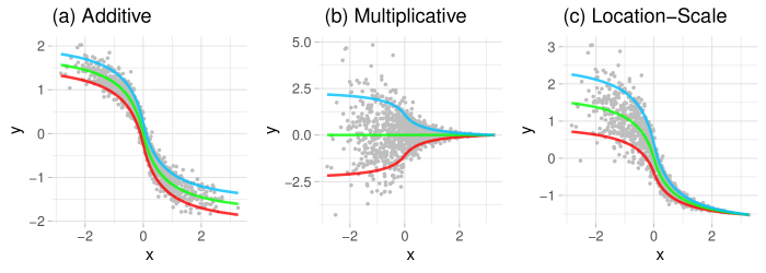
Figure 1: Diverse cause-effect ($X\rightarrow Y$) setups. Green - median, blue - $0.9^{th}$ quantile, red - $0.1^{th}$ quantile. Focusing on the mean only is not enough in the location-scale and multiplicative cases.

In Figure 1, we illustrate a limitation of causal inference methods based on the conditional mean and refer to Section 2.2 for more details on the underlying generative mechanisms. From Figure 1(a), it is clear that the variance of the effect variable is independent of the cause. As a result, the independence between the cause and the effect’s noise can be measured in various ways by substracting an estimate of the conditional mean. In Figure 1(b) and (c) however, the mechanisms are $Y=g(X)N_{Y}$ and $Y=f(X)+g(X)N_{Y}$ respectively. In other words, the variance of the effect also depends on the cause, i.e. it exhibits heteroskedasticity. Assume that $E(N_{Y})=0$, then in the multiplicative case, we have that $E(Y|X=x)=0$. And it is not sensible to use the conditional mean to identify the causal direction. But since $\mbox{Var}(Y|X=x)=x^{2}$, the variance is more informative. Similarly, features of the conditional distributions (e.g., conditional spread) different from the location might help. In such cases, relying on mutliple (conditional) quantiles rather than on the mean only can help. As we show in Section 3, it allows us to correctly determine the causal direction across various benchmarks where additive-noise competitors fail when their assumptions are not met.

A classic example of real world data displaying such features is the impact of income on expenditure on meals: as an individual’s income increases, so does its food expenditure and food expenditure variability. An explanation could be as follows: while a poorer person will spend a rather constant amount on inexpensive food, wealthier individuals occasionally buy inexpensive food and sometimes eat expensive meals. Or, that wealthier individuals have more leeway when deciding which fraction of their income to allocate to food expenditure, whereas poorer ones are constrained by necessity. This heteroskedastic effect can be observed in Figure 2, where our method use multiple quantiles to find the correct causal direction.

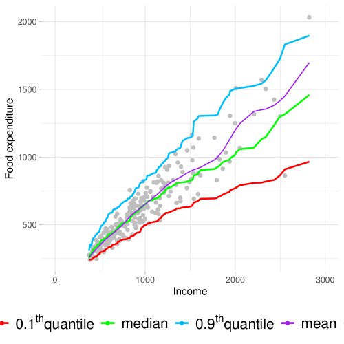
Figure 2: Heteroskedasticity in food expenditure as a function of income for Belgian working class households. Our method uses multiple quantiles to find the correct causal direction.

Another line of work avoids functional restrictions by relying on the independence of cause and mechanism postulate (Schölkopf et al., 2012; Peters et al., 2017).

Postulate 1 (Sgouritsa et al. 2015).

The marginal distribution of the cause and the conditional distribution of the effect given the cause, corresponding to independent mechanisms of nature, are algorithmically independent (i.e., they contain no information about each other).

Information Geometric Causal Inference (IGCI) (Janzing et al., 2012) uses the postulate directly for causal discovery. Similarly, Regression Error based Causal Inference (RECI) (Blöbaum et al., 2018) develops structural assumptions based on the postulate to imply that, if $X$ causes $Y$ implies an asymmetry in mean-regression errors, that is

$$E[(Y-E[Y|X])^{2}]\leq E[(YX-E[X|Y])^{2}].$$ (1)

Alternatively, (Mooij et al., 2009; Janzing & Schölkopf, 2010) reformulate the postulate through asymmetries in Kolmogorov complexities (Kolmogorov, 1963) between marginal and conditionals distributions. However, the halting problem (Turing, 1938) implies that the Kolmogorov complexity is not computable, and approximations or proxies have to be derived to make the concept practical.

In this context, (Mooij et al., 2010) proposes a method based on the minimum message length principle using Bayesian priors, while others are based on reproducing kernel Hilbert space embedding such as EMD (Chen et al., 2014), FT (Liu & Chan, 2017) and KCDC by Mitrovic et al. (2018), or using entropy as a measure of complexity (Kocaoglu et al., 2017). A related line of work suggests using the minimum description length (MDL, Rissanen, 1978) principle as a proxy for Kolmogorov complexity: (Budhathoki & Vreeken, 2017) uses MDL for causal discovery on binary data, and Slope (Marx & Vreeken, 2017, 2019) implements (local and) global functional relations using MDL based regression and is suitable for continuous data.

In this paper, we build on a similar idea, using quantile scoring as a proxy for the Kolmogorov complexity through the MDL principle. We develop a method leveraging asymetries similar to (1), replacing the squared loss and conditional mean by the pinball loss and conditional quantiles. To the best of our knowledge, quantiles have only been mentioned in a somewhat related context by (Heinze-Deml et al., 2018), where quantile predictions are used to exploit the invariance of causal models across different environments. As opposed to (Heinze-Deml et al., 2018), our method uses an asymmetry directly derived from the postulate, and therefore it does not require an additional variable for the environment.

To avoid the restrictive assumptions imposed by standard quantile regression techniques (e.g., linearity of the quantiles or additive relationships), we suggest fully nonparametric bQCD implementations using three different approaches: copulas, quantile forests or quantile neural networks. We also show that bQCD is robust to the choice regression approach. To the best of our knowledge, we are the first to explore the idea of using conditional quantiles to distinguish cause from effect in bivariate observational data. Our main contributions are:

• a new method based on quantile scoring to determine the causal direction without any assumptions on the class of causal mechanisms along with a theoretical analysis justifying its usage (Section 2),

• quantile causal discovery (bQCD), an efficient implementation robust to the choice of underlying regressor (Section 3.1),

• a new benchmark set of synthetic cause-effect pairs from additive, location-scale and multiplicative noise models (Section 3.2),

• a comparative study to benchmark bQCD against state-of-the-art alternatives (Section 3).

2 Causal Discovery using Quantiles

In this section, we develop our quantile-based method for distinguishing between cause and effect from continuous and discrete observational data.

Problem setting We restrict ourselves to bivariate cases by considering pairs of univariate random variables. We further simplify the problem by assuming the existence of a causal relationship but the absence of confounding, selection bias, and feedback.

2.1 Kolmogorov Complexity and Quantile Scoring

Let $X$ and $Y$ be two random variables with some joint distribution $F$, and where $F_{X},F_{Y}$ and $F_{Y\mid X},F_{X\mid Y}$ are respectively the marginal and conditional distributions. The Kolmogorov complexity of a distribution $F$, denoted by $K(F)$, is the length of the shortest program $p$ that outputs $F(x)$ up to precision $q$ for all $x$, that is

$$K(F)=\min\left\{\mid p\mid\,:\,\mid U(p,q,x)-F(x)\mid\leq 1/q,\,\forall x\right\},$$

with $U$ a Turing machine extracting $p(x,q)$ (see Janzing & Schölkopf, 2010, and references therein).

In our setting, the Kolmogorov complexity can be leveraged to discover which one of $X$ and $Y$ is the cause and which one is the effect through the following theorem:

Theorem 1 (Mooij et al. 2010).

If Postulate 1 holds and $X$ causes $Y$, then $K(F_{X})+K(F_{Y|X})\leq K(F_{Y})+K(F_{X|Y})$.

Stated differently, the causal direction between $X$ and $Y$ can be recognized as the least complex, that is the decomposition of the joint distribution leading to the lowest value of the Kolmogorov complexity. This is because, in this context, the direct translation of Postulate 1 is that the mutual information between $F_{X}$ and $F_{Y|X}$ equals zero while that between $F_{Y}$ and $F_{X|Y}$ does not. In other words, the number of bits saved when compressing $X$ and $Y$ jointly rather than compressing them independently is smaller when using the causal factorization of the joint distribution. Importantly, because we assumed the existence of a causal link, the asymmetry in Theorem 1 is not only necessary but also sufficient.

Remark 1.

Note that our problem setting corresponds to assumptions A, B and C in (Mooij et al., 2010). Furthermore, Theorem 1 holds up to an additive constant, as the asymmetry does not depend on the strings involved, but may depend on the Turing machines they refer to (see e.g., Janzing & Schölkopf, 2010; Hernández-Orallo & Dowe, 2010). When using the same Turing machine to compute all complexities, carrying this constant over is not required.

Since the Kolmogorov complexity is not computable, we use the MDL principle (Rissanen, 1978) as a proxy: the less complex direction becomes the one allowing a better compression of the data. In other words, the correct causal direction allows to store information using the shortest description length, or code length (CL).

Two-step MDL encoding To construct a coding scheme satisfying the MDL principle, we use a two-stage approach (see e.g., Hansen & Yu, 2001, Section 3.1): first encode a model and then the data using that model. Assume that the goal is to compress $X=\left\{X_{i}\right\}_{i=1}^{n}$ with $X_{i}\in\mathcal{X}$ i.i.d. according to some distribution $F_{X}\in\mathcal{F}$, where the model class is known to be $\mathcal{F}=\left\{f_{\theta}(\cdot)\mid\theta\in\Theta\right\}$ and $\theta$ is an indexing parameter. When $\theta$ is known, Shanon’s source coding theorem implies that an encoding based on $f_{\theta}$ is “optimal”: on average, it achieves the lower bound on any lossless compression, that is the differential entropy $-n\int_{\mathcal{X}}f_{\theta}(z)\log f_{\theta}(z)dz$. And the code length of a dataset encoded using the known $f_{\theta}$ is given by minus its log-likelihood $\mbox{CL}(X\mid\theta)=-\sum_{i=1}^{n}\log f_{\theta}(X_{i})$. This optimal scheme thus amounts at transmitting the true parameter along with the data encoded using its known distribution:

$$\mbox{CL}_{\theta}(X)=\mbox{CL}(\theta)+\mbox{CL}(X\mid\theta),$$ (2)

where the two terms on the right-hand side result from transmitting the model and the data encoded using the model (see e.g., Hansen & Yu, 2001, Section 3.1).

Encoding marginals via quantiles Since knowledge of the model class and true parameter is seldom achieved, consider compression using partial information about the data-generating process. Assuming that we only know a $\tau$-quantile $q_{X,\tau}=\operatorname{arg\,inf}_{q}\left\{q\mid F_{X}(q)=\tau\right\}$, we can compress the data by transmitting $\tau$, $q_{X,\tau}$, and the “residuals” $E_{X}=\{X_{i}-q_{X,\tau}\}_{i=1}^{n}$. This encoding results in

$$\mbox{CL}_{\tau}(X) =\mbox{CL}(\tau)+\mbox{CL}(q_{X,\tau})+\mbox{CL}(E_{X}\mid q_{X,\tau},\tau).$$ (3)

To encode $E_{X}$, it is then natural to use the asymmetric Laplace (AL) distribution (see Aue et al., 2014; Geraci & Bottai, 2007; Yu et al., 2003) with density $f(z;q,\tau)=\tau(1-\tau)\exp(-S_{\tau}(q,z))$, where $S_{\tau}(\cdot,\cdot)$ is the quantile scoring (QS) function

$$S_{\tau}(x_{1},x_{2})=(\mathbb{I}\left\{x_{1}\geq x_{2}\right\}-\tau)(x_{1}-x_{2}).$$

Given that the distribution of $E_{X}$ is generally unknown, using the AL is optimal in the sense that the population quantile is exactly the minimizer of the QS’s expected value, namely $q_{X,\tau}=\mbox{argmin}_{q}\,\mathbb{E}\left[S_{\tau}(q,X)\right]$. We revisit the link between QS and the AL in Section 2.2.

Using this encoding, the last term in the right-hand side of (3) is finally given by the negative of the AL log-likelihood (Rissanen, 1986), that is

$$\mbox{CL}(E_{X}\mid q_{X,\tau},\tau)=\sum_{i=1}^{n}S_{\tau}(q_{X,\tau},X_{i})-a_{n}(\tau),$$ (4)

where $a_{n}(\tau)=n\log(\tau(1-\tau))$.

Encoding conditionals via quantiles Next, consider the problem of compressing $\left\{X_{i},Y_{i}\right\}_{i=1}^{n}$ with $(X_{i},Y_{i})$ i.i.d. according to some joint distribution $F$. Because $F$ can be decomposed using the marginal and the conditional distributions, one can proceed as above with $F_{X}$ to compress $X$, and then use $F_{Y\mid X}$ to compress $Y$ given $X$. Assume similarly that the only information about the conditional data-generating process is the conditional $\tau$-quantile $q_{Y\mid X=x,\tau}=\operatorname{arg\,inf}_{q}\left\{q\mid F_{Y\mid X=x}(q)=\tau\right\}$ of $Y$ given $X=x$. Encoding a conditional distribution using (3) and (4) thus results in

$$\mbox{CL}_{\tau}(Y\mid X) =\mbox{CL}(\tau)+\mbox{CL}(q_{Y\mid X,\tau})$$ (5)

$$\phantom{=}+\sum_{i=1}^{n}S_{\tau}(q_{Y\mid X=X_{i},\tau},Y_{i})-a_{n}(\tau).$$

In other words, the data is compressed by transmitting $\tau$, $q_{Y\mid X,\tau}$, and the “residuals” $E_{Y\mid X}=\{Y_{i}-q_{Y\mid X=X_{i},\tau}\}_{i=1}^{n}$. Note that, for a given fixed quantile level $\tau$, while $q_{X,\tau}$ is a real number, $q_{Y\mid X,\tau}$ is generally a function of the conditioning variable.

Causal identification via quantiles The same idea can be applied to compress the data with the decomposition of the joint distribution $F$ using the marginal $F_{Y}$ and the conditional $F_{X\mid Y}$ distributions. But according to Theorem 1 and using CLs as proxies for Kolmogorov complexities, if $X$ is a cause of $Y$, one expects that for all $\tau\in(0,1)$

$$\mbox{CL}_{\tau}(X)+\mbox{CL}_{\tau}(Y\mid X)\leq\mbox{CL}_{\tau}(Y)+\mbox{CL}_{\tau}(X\mid Y)$$

with high probability as the sample size increases. We thus make the following “identifying” assumption for $X$ to be a cause of $Y$:

Assumption 1.

$P\left(\frac{\mbox{CL}_{\tau}(X)+\mbox{CL}_{\tau}(Y\mid X)}{\mbox{CL}_{\tau}(Y)+\mbox{CL}_{\tau}(X\mid Y)}\leq 1\right)\underset{n\to\infty}{\longrightarrow}1$

This assumption is called identifying because, if the ratio of CLs equals 1 for all $\tau\in\left(0,1\right)$, quantile-based CLs cannot be leveraged for causal discovery. For any given sample size and quantile level $\tau$, cases where $\mbox{CL}(\tau)=\infty$, $\mbox{CL}(q_{X,\tau})=\infty$ or $\mbox{CL}(q_{Y\mid X,\tau})=\infty$ are problematic. The issue can be resolved by assuming for instance that all population quantities are computable and can be transmitted using a finite albeit potentially increasing precision.

Using $O$/$o$ for the usual asymptotic notations, we draw a first link between CLs and QSs at the population level.

Theorem 2.

Assume that $\mbox{CL}(l)=o(n)$ for $l\in\{\tau,q_{X,\tau},q_{Y,\tau},q_{Y|X,\tau},q_{X|Y,\tau})\}$, then Assumption 1 holds if and only if

$$\frac{\mathbb{E}\left[S_{\tau}(q_{X,\tau},X_{i})\right]+\mathbb{E}\left[S_{\tau}(q_{Y\mid X=X_{i},\tau},Y_{i})\right]}{\mathbb{E}\left[S_{\tau}(q_{Y,\tau},Y_{i})\right]+\mathbb{E}\left[S_{\tau}(q_{X\mid Y=Y_{i},\tau},X_{i})\right]}\leq 1.$$ (6)

Because the population (conditional) quantiles and the expectations involved in the ratio are seldom known in practice, Theorem 2 cannot be leveraged directly for causal discovery. However, it can be used to determine whether a given causal model satisfies Assumption 1, as exmplified below. The proof can be found in Section A.1.

Example 1.

Consider $X$ being a cause of $Y$ in the linear model defined by $X=\theta_{1}N_{X}$ and $Y=\gamma X+\theta_{2}N_{Y}$ with $N_{X}$ and $N_{Y}$ two independent sources of noise and $\theta_{1},\theta_{2},\gamma>0$ such that $\mbox{var}(X)=\mbox{var}(Y)$. Note that the condition on the variances simply ensures that the variables have the same scale.

Letting $N_{X},N_{Y}\sim N(0,1)$, $X\sim N(0,\theta_{1}^{2})$ and $Y\sim N(0,\gamma^{2}\theta_{1}^{2}+\theta_{2}^{2})$. The variance equality condition can be satisfied by choosing $\gamma\in(0,1)$ and letting $\theta_{2}=\theta_{1}\sqrt{1-\gamma^{2}}$, resulting in $X\mid Y=y\sim N(\gamma y,(1-\gamma^{2})\theta_{1}^{2})$ and $Y\mid X=x\sim N(\gamma x,(1-\gamma^{2})\theta_{1}^{2})$. Using the fact that, if $Z\sim N(\mu,\sigma)$, then $\mathbb{E}\left[S_{\tau}(q_{Z,\tau},Z)\right]=\sigma c(\tau)$, where $c(\tau)=e^{-\Phi^{-1}(\tau)^{2}/2}/\sqrt{2\pi}$ with $\Phi$ the standard normal cumulative distribution, it is then straightforward to verify that the ratio of expectations in Theorem 2 is equal to one independently of $\tau$. In other words, the linear Gaussian model is not identifiable (Shimizu et al., 2006; Hoyer et al., 2009; Peters et al., 2014).

Remark 2.

Developing structural or distributional assumptions, e.g. based directly on Postulate 1, such that Assumption 1 or (6) holds is an open problem. (Blöbaum et al., 2018) paves the way in the context of (1) and in the regime of almost deterministic relations. But quantiles and quantile scores are harder to manipulate than conditional variances and squared losses.

Causal discovery via quantiles In order to leverage Assumption 1 for causal discovery, we let $\widehat{q}_{X,\tau}$, $\widehat{q}_{Y,\tau}$, $\widehat{q}_{X|Y,\tau}$, $\widehat{q}_{Y|X,\tau}$ be estimators of the respective population quantiles, and further make the following assumption:

Assumption 2.

$\widehat{q}_{X,\tau}$, $\widehat{q}_{Y,\tau}$, $\widehat{q}_{X|Y,\tau}$, $\widehat{q}_{Y|X,\tau}$ satisfy

• $\left|\widehat{q}_{X,\tau}-q_{X,\tau}\right|=o_{p}(1)$ and $\left|\widehat{q}_{Y,\tau}-q_{Y,\tau}\right|=o_{p}(1)$,

• $\left|\widehat{q}_{Y\mid X=x,\tau}-q_{Y\mid X=x,\tau}\right|=o_{p}(1)$ for every $x$ and
  $\left|\widehat{q}_{X\mid Y=y,\tau}-q_{X\mid Y=y,\tau}\right|=o_{p}(1)$ for every $y$,

• $\mbox{CL}(\widehat{q}_{X,\tau})=o(n)$, $\mbox{CL}(\widehat{q}_{Y|X,\tau})=o(n)$,
  $\mbox{CL}(\widehat{q}_{Y,\tau})=o(n)$, and $\mbox{CL}(\widehat{q}_{X|Y,\tau})=o(n)$,

using $O_{p}$/$o_{p}$ for stochastic boundedness and convergence in probability.

The first two bullet points simply state that the unconditional and conditional quantile estimators are consistent without rate. As for the third bullet point, note that having the same growth rate for the CL of all models does not prevent a smaller number of parameters in the correct causal direction (see e.g., Blöbaum et al., 2018; Marx & Vreeken, 2019). However, it means that, if the population quantiles $q_{\cdot,\tau}$ are replaced by estimators $\widehat{q}_{\cdot,\tau}$ in (3) and (5), the CLs of the models are all asymptotically dominated by the CLs of the residuals, namely the $\sum_{i=1}^{n}S_{\tau}(\cdot,\cdot)$ terms.

The third bullet point of Assumption 2 includes the important case where all CLs are $O(\log n)$ (Rissanen, 1983, 1986): discretizing a compact parameter space with a $n^{-1/2}$ grid (i.e., the magnitude of the estimation error) and transmitting an estimated parameter using a uniform encoder with this precision is optimal for regular parametric families. Using this $n^{-1/2}$ precision, each parameter thus leads to a cost of $1/2\,\log n$.

For nonparametric (i.e., with a non-Euclidean parameter space) models, a similar idea can be applied, as estimators typically converge at a rate slower than $n^{-1/2}$. For instance, it is well known that the optimal grid size for histogram estimators of continuous densities with bounded first derivative is proportional to $n^{-1/3}$ (Theorem 6.11, Wasserman, 2006). And if each of the histogram heights is encoded using $n^{-1/2}$ grid (i.e., smaller than the estimation error), the resulting estimator’s CL is proportional to $n^{1/3}/2\,\log n$, which satisfies the third bullet point of Assumption 2. More generally, the fastest possible rate for kernel density estimators of continuous densities with $k$ bounded derivatives is $n^{k/(2k+1)}$ (Theorem 6.31, Wasserman, 2006). As a result, discretizing the support on a grid proportional to $n^{-k/(2k+1)}$ and encoding the kernel values using a $n^{-1/2}$ grid encures an estimator’s CL proportional to $n^{k/(2k+1)}/2\,\log n$.

However, Assumption 2 excludes datasets where quantiles can only be consistently estimated with models having “too many parameters”. For instance, if the only consistent estimator is an over-parametrized neural network with $o(n_{layers}\times n_{neurons/layer})>o(n)$, then Assumption 2 does not hold. But such a situation is unlikely in our bivariate setting.

We can then state the following theorem:

Theorem 3.

Under Assumption 2, Assumption 1 holds if and only if

$$P\left(\frac{S_{X,\tau}+S_{Y\mid X,\tau}}{S_{Y,\tau}+S_{X\mid Y,\tau}}\leq 1\right)\underset{n\to\infty}{\longrightarrow}1,$$

with the scores $S_{X,\tau}=\sum_{i=1}^{n}S_{\tau}(\widehat{q}_{X,\tau},X_{i})$, $S_{Y\mid X,\tau}=\sum_{i=1}^{n}S_{\tau}(\widehat{q}_{Y\mid X=X_{i},\tau},Y_{i})$ and similarly for $Y$ and $X\mid Y$.

Note that Theorem 3 does not state that CLs and QSs are equivalent, but rather that inequalities in CLs imply inequalities in QSs with respect to a specific statistical model, and conversely. In other words, Theorem 3 implies that there is an equivalence between minimizing code length and quantile score. Hence, because of the MDL principle, the causal direction can be inferred from the lowest quantile score. The proof can be found in the supplementary material (Section A.2), but the intuition is as follows.

Because of the third bullet point in Assumption 2, QSs, namely the CLs of the residuals, asymptotically dominate the CLs of the models. As a result, using QSs corresponding to consistent models is sufficient for causal discovery.

Thanks to the stability (or invariance) of the true causal model, we expect Assumption 1 to hold over different quantile levels. However, since a single quantile is generally not enough to characterize a distribution, we further consider

$$\widehat{S}_{X}=\int_{[0,1]}S_{X,\tau}d\tau,$$ (7)

and similarly for $X\mid Y$, $Y$ and $X|Y$. By pooling results at different quantile levels, we aim at better describing the marginal and conditional distributions. Arguing that estimating high and low (conditional) quantiles is hard, we could use only quantiles close to the median, that is integrating between over $[0.4,0.6]$ instead of $[0,1]$). We empirically found that this was more error prone when the generative models have asymmetries or multiplicative noises. Finally, we use averaging through integration rather than the maximal QS difference over quantile levels because the scale of QS is not uniform (e.g., the closer to 0.5 the higher). Hence, using maximization would essentially mean basing the decision on the median only, whereas properly capturing the spread of the data is also important.

Decision rule 1 (Bivariate Quantile Causal Discovery).

Let $S_{X\to Y}=\widehat{S}_{X}+\widehat{S}_{Y|X}$ and $S_{Y\to X}=\widehat{S}_{Y}+\widehat{S}_{X|Y}$ If $S_{X\to Y}<S_{Y\to X}$, conclude that $X$ causes $Y$. If $S_{X\to Y}>S_{Y\to X}$, conclude that $Y$ causes $X$. Otherwise, do not decide.

2.2 Intuition

The mean and squared loss duality leads to using the MSE as a metric for mean regression even for non-Gaussian data. And the pinball loss plays a similar role in quantile regression. In the MDL paradigm, the optimal encoding uses the data’s true distribution, which is usually unkown for the residuals of either a mean or quantile regression. Without knowing this optimal encoding, it is sensible to use a distribution related to the loss that is minimized. A Gaussian or asymmetric Laplace (AL) encoding should thus not be seen as optimal, but as a “default” related to the specific mean or quantile regression problem. Furthermore, a Gaussian encoding is unlikely to be appropriate for quantile residuals, which are often asymmetrically distributed.

To make this idea more precise, consider (1), albeit from the point of view of the MDL principle. One seeks a model that allows the best compression of the data, measured in code length (CL). Using a two-part scheme as in (2), the total CL is the sum of the conditional mean’s CL and that of the residuals, which is equal to the negative log-likelihood of the distribution used to encode them. And encoding the residuals using the normal distribution is natural in the same sense as using the mean squared error as a regression metric. The reason is that minimizing the squared loss is equivalent to maximizing the Gaussian log-likelihood, thus minimizing the residuals’ CL.

A similar reasoning can be applied to quantile regression, where encoding the residuals using an AL distribution (Koenker & Machado, 1999) represents a sensible default. This is because minimizing the quantile score (QS) is equivalent to maximizing the AL log-likelihood ($a_{n}(\tau)-\mbox{QS}$), thus minimizing the residuals’ CL. Intuitively, the likelihood corresponding to (conditional) residuals in the causal direction is higher, that is the QS and CL are smaller: the shortest CL corresponds to the largest AL likelihood/smallest QS, which establishes a link between minimizing QS and the MDL principle.

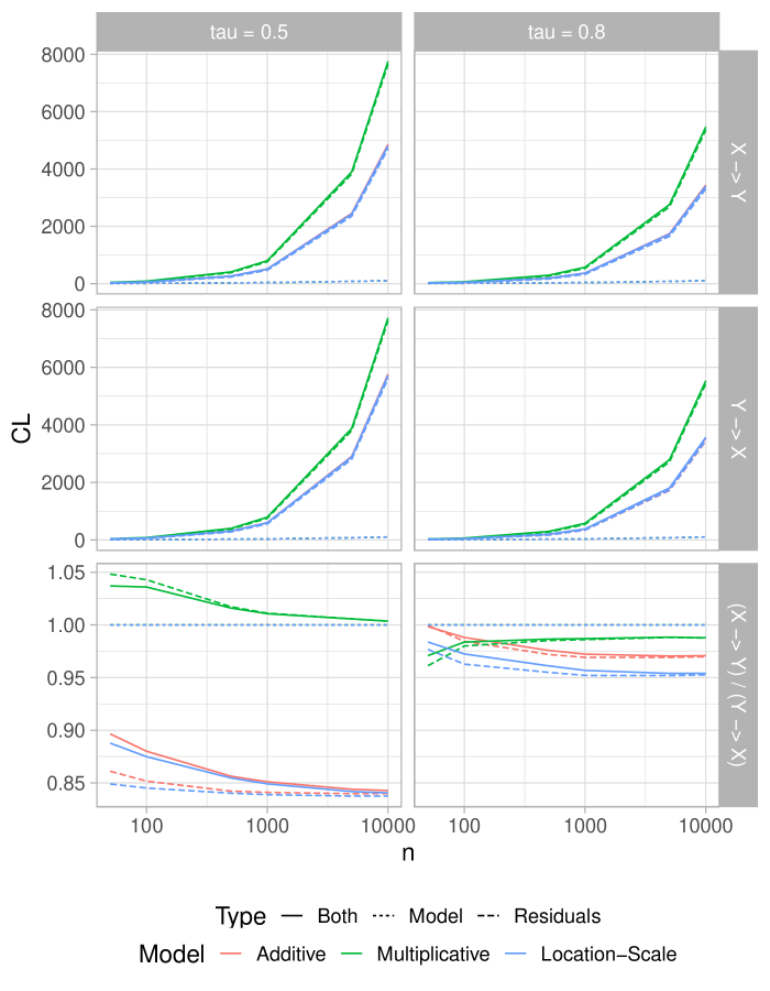
Figure 3: Verifying Assumption 1 for the setups of Figure 1. The CLs of the residuals asymptotically dominate the CLs of the marginal and conditional models. The multiplicative model is not identifiable using the median only. The correct causal direction has a lower CL.

Let us now illustrate the key ideas in the theoretical justification of bQCD. In Figure 3, we revisit the toy examples from Figure 1, namely, the different setups: additive, multiplicative and location-scale causal pairs. We disentangle the CL’s different components for both the causal $X\rightarrow Y$ and anti-causal $Y\rightarrow X$ direction, for two quantile levels $\tau\in\{0.5,0.8\}$ and per generative model.

Curves are obtained by averaging over 100 repetitions.

As described in Section 2.1, causal discovery by MDL involves four summands for each possible direction. For instance, for $X\to Y$, we have

• two for the marginal and conditional model parameters, $\mbox{CL}(\widehat{q}_{X,\tau})$ and $\mbox{CL}_{\tau}(\widehat{q}_{Y\mid X,\tau})$,

• and two for the marginal and conditional residuals, $\mbox{CL}(E_{X}\mid\widehat{q}_{X,\tau},\tau)$ and $\mbox{CL}(E_{X|Y}\mid\widehat{q}_{X|Y,\tau},\tau)$.

In Figure 3, we use Model for the former and Residuals for latter and sum them by type. The sum of both model and residuals CLs is given by full lines. Unconditional and conditional quantiles are estimated respectively using the empirical quantile and kernel quantile regression. A uniform encoding is assumed in both cases, resulting in respective model CLs of $1/2\log(n)$ and $n^{1/3}/2\log(n)$.

In the top four panels of Figure 3, it is clear that the CLs of the residuals (i.e., the QSs) dominate the CLs of the marginal and conditional models. This illustrates the third bullet point in Assumption 2.

In the bottom two panels of Figure 3, we see that the ratio of causal to anti-causal CLs generally converges to some constant smaller than 1, which illustrates Assumption 1. It also means that Decision rule 1 would lead to the correct causal direction. The multiplicative noise mechanism has an interesting behaviour: considering the median only (i.e., $\tau=0.5$), the ratio converges slowly to one, and therefore, the causal direction is not identifiable. However given that the ratio converges to some constant smaller than one for $\tau=0.8$, pooling the decision over multiple quantiles as in Decision rule 1 would again lead to the correct causal direction.

3 Experiments

3.1 bQCD implementation

Quantile regression Theorem 3 holds provided that the model is consistent and its complexity does not grow too fast. As such, Decision rule 1 can be implemented using any quantile regression approach that satisfies Assumption 2. In our experiments, we use three methods, namely nonparametric copulas (Geenens et al., 2017), quantile forests (Meinshausen, 2006), quantile neural networks (Cannon, 2018), and show that they yield qualitatively and quantitatively similar results. We refer to Appendix B for more details on the regression methods and their specific implementations.

For estimating the overall quantile scores (aggregating multiple quantile levels), we use Legendre quadrature to approximate the integral over $[0,1]$, as it is fast and precise for univariate functions. In other words, denoting by $\left\{w_{j},\tau_{j}\right\}_{j=1}^{m}$ the $m$ pairs of quadrature weights and nodes, we use $\int_{0}^{1}g(\tau)d\tau\approx\sum_{j=1}^{m}w_{j}g(\tau_{j})$, which when plugged into (2.1) yields $\widehat{S}_{X}=\sum_{j=1}^{m}w_{j}\widehat{S}_{X}(\tau_{j})$, $\widehat{S}_{Y}=\sum_{j=1}^{m}w_{j}\widehat{S}_{Y}(\tau_{j})$, $\widehat{S}_{X|Y}=\sum_{j=1}^{m}w_{j}\widehat{S}_{X|Y}(\tau_{j})$, and $\widehat{S}_{Y|X}=\sum_{j=1}^{m}w_{j}\widehat{S}_{Y|X}(\tau_{j})$. Summing over an equally spaced grid with uniform weights or using quadrature nodes and weights yields two valid approximations of an integral, and using one or the other should not matter. But the quadrature gives more importance to the center of the distribution (i.e., quantiles closer to 0.5 have a higher weight). Note that, to compute scores free of scale bias, the variables are transformed to the standard normal scale.

Computational complexity bQCD scales linearly with the size of input data, $O(n)$ for copulas, $O(n_{tree}\times n_{attr}\times depth\times n)$ for random forests and $O(epochs\times n_{weights}\times n)$ corresponding to the choice of regressor. However, using multiple quantile levels does not increase the complexity significantly since all of the suggested implementations allow for simultaneous conditional quantile estimation, that is, we estimate a single model at each possible causal direction , from which we compute all of the requested quantiles. Roughly speaking, since $n>>m$, the overall complexity scales with $\mathcal{O}(n)$. As such, bQCD compares favorably to nonparametric methods relying on computationally intensive procedures, for an instance based on kernels (Chen et al., 2014; Hernández-Lobato et al., 2016) or Gaussian processes (Hoyer et al., 2009; Mooij et al., 2010; Sgouritsa et al., 2015).

The parameter $m$ can be used to control for the trade-off between the computational complexity and the precision of the estimation. We recommend the value $m=3$ which, makes it possible to capture variability in both location and scale. Setting $m=1$ is essentially equivalent to using only the conditional median for causal discovery, a setting that suitable for distributions with constant variance. An empirical analysis of the choice of $m$ is provided in the following section. In what follows, we report results for bQCD with $m=3$ if not stated otherwise.

3.2 Datasets, baselines and metrics

Benchmarks For simulated data, we first rely on the following scenarios (Mooij et al., 2016): SIM (without confounder), SIM-ln (with low noise), SIM-G (with distributions close to Gaussian), and SIM-c (with latent confounder). There are 100 pairs of size $n=1000$ in each of these datasets.

As a second benchmark, inspired by (Peters et al., 2014), we generate a diverse dataset of additive, location-scale and multiplicative causal pairs. We include nonlinear additive noise (AN) models of the form $Y=f(X)+E_{Y}$ for some deterministic function $f$ with $E_{Y}\sim{\cal{N}}(0,\sigma)$, $X\sim{\cal{N}}(0,\sqrt{2})$, and $\sigma\sim{\cal{U}}[1/5,\sqrt{2/5}]$. In AN, $f$ is an arbitrary nonlinear function simulated using Gaussian processes (GP, Rasmussen & Williams, 2006) with a Gaussian kernel of bandwidth one. Since the functions in AN are often non-injective, we include AN-s to explore the behavior of bQCD in injective cases. In this setup, $f$ are sigmoids as in (Bühlmann et al., 2014). The third experiment considers location-scale (LS) data generating processes with both the mean and variance of the effect being functions of the cause, that is $Y=f(X)+g(X)E_{Y}$, and $E_{Y}$ and $X$ are similar as for the additive noise models. LS and LS-s then correspond to the Gaussian processes and sigmoids described for AN and AN-s. Finally, the fourth experiment considers multiplicative models (MN) as $Y=f(X)E_{Y}$, with $f(X)$ sampled as sigmoid functions and $E_{Y}\sim{\cal{U}}(0,1)$. In each of the second, third, and fourth experiments, we simulate 100 pairs of size $n=1000$. All pairs have equal weights with variable ordering according to a coin flip, therefore resulting in balanced datasets. Example datasets for each of the simulated experiments are shown in the supplementary material (Appendix F).

For real data, we use the Tübingen CE benchmark (version Dec 2017), consisting of 108 pairs from 37 different domains, from which we consider only the 99 pairs that have univariate continuous or discrete cause and effect variables. When evaluating the performance on this dataset we included the pairs’ corresponding weights which accounts for potential bias in cases where pairs were selected from same multivariable dataset.

Baselines On simulated data, we compare bQCD to state-of the-art approaches, namely RESIT (Peters et al., 2014), biCAM (Bühlmann et al., 2014), LinGaM (Shimizu et al., 2006), and GR-AN (Hernández-Lobato et al., 2016), which are ANM-based, and IGCI (Janzing & Schölkopf, 2010), EMD (Chen et al., 2014), RECI (Blöbaum et al., 2018), Slope (Marx & Vreeken, 2017) and Sloppy (Marx & Vreeken, 2019), based on the independence postulate. We also consider other methods such as PNL-MLP (Zhang & Hyvärinen, 2009), GPI (Mooij et al., 2010), ANM (Hoyer et al., 2009), and CURE (Sgouritsa et al., 2015). All baselines distinguish between cause and effect solely in the bivariate case, except for CAM, RESIT and LinGaM whose impementations allow for higher dimensional causal discovery. Implementation details and hyper parameters for all baselines are described in the supplementary material (Section C.1).

Our code and datasets are available in the submitted supplementary package and https://github.com/tagas/bQCD.

Evaluation metrics As (Mooij et al., 2016), we use the accuracy for forced decisions and the area under the receiver operating curve (ROC) for ranked decisions. The former corresponds to forcing the compared methods to decide the causal direction. The later corresponds to using heuristic scores allowing to rank confidence in the directions along with ROC/AUC as performance measure. As a confidence heuristic for the ranked decisions for bQCD, we use same score as (24) in (Mooij et al., 2016), that is $\hat{C}=-S_{X\to Y}+S_{Y\to X}$, with higher absolute values corresponding to higher confidence. This score can also be paired with the null-hypercompressibility inequality (Grünwald & Grunwald, 2007) to derive a significance test and abstain from making insignificant inferences.

3.3 Results and discussion

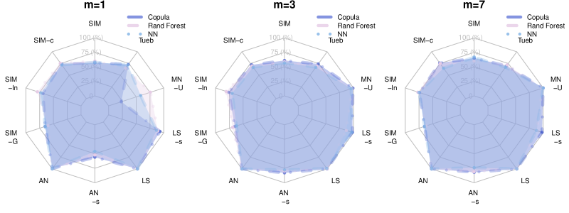
Figure 8: bQCD robustness with respect to implementation for different number quantiles.

bQCD robustness wrt to its implementation From Figure 4 it is clear that the choice of implementation in estimating the conditional quantiles has no significant impact and bQCD provides consistent results across all benchmarks. Further results that confirm the robustness to implementation for different values of $m$ are shown in Appendix B, Figure 8. In the remaining of the paper we will show the copula-based results.

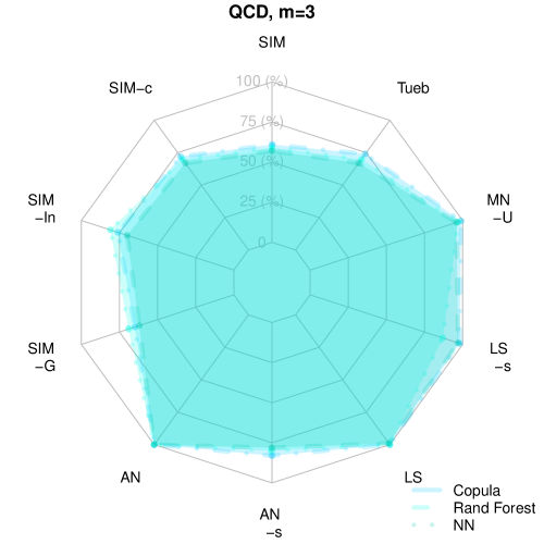
Figure 4: bQCD achieves consistent results across all benchmarks regardless of the practical implementation.

Selection of $m$ In an ablation study we explored the significance of the parameter $m$ with regards to different sample sizes. Looking at the figures in Figure 5, we can clearly see in which cases multiple quantile levels can indeed increase the accuracy, namely for sigmoid (i.e., harder to detect) causal mechanisms. For confounded data, increasing $m$ seems to help too, albeit faintlier. Additionally, we can notice that higher values of $m$ have more pronounced effect as the sample size increases. This was used to improve our results on real data, namely by setting the parameter $m$ to 1 when $n<200$ and $m=3$ for the rest.

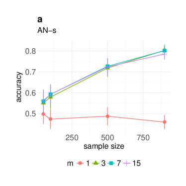
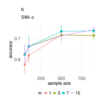
Figure 5: The accuracy increases with $m$ and the sample size.

Comparison to baselines In Figure 6, we compare causal discovery algorithms across simulated datasets with regards to accuracy. Tabulated numbers are in Section D.1.

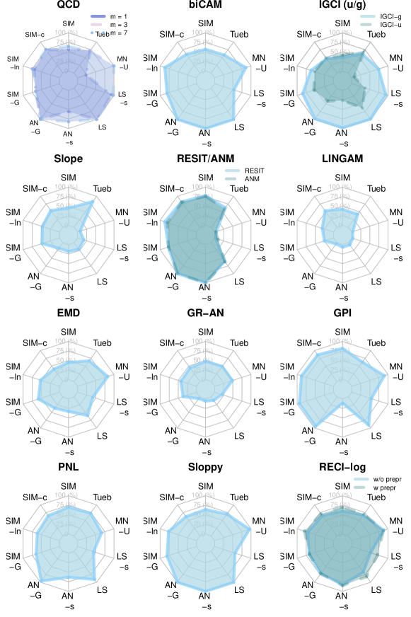
Figure 6: Accuracy of bQCD and competitors.

There is no single baseline is an overall best performer, however, we notice that bQCD has most consistent results across all benchmarks. Starting with the SIM benchmarks, we notice that GPI achieves highest accuracy in all four scenarios, followed with similar results by RESIT/ANM . On this benchmark, bQCD behaves similarly to the rest of the baselines, while being more robust in the confounded scenario where others achieve results on the scale of random guess. Interestingly, higher values of the parameter $m$ improve the results in such pairs.

The results are significantly different for the AN, LS and MN scenarios. biCAM, ANM and RESIT easily handle the AN pairs since their underlying assumptions are met, while we can notice some discrepancy in the LS and MN scenarios where there is an interaction between the noise and the cause. Similarly, LINGAM does not perform well on any of the datasets, which are all highly nonlinear, hence violating its assumptions. IGCI can handle any scenario with the gaussian reference measure, while this is not the case with the uniform measure. In the LS generative models where not only the mean, but the variance of the effect changes with the cause only IGCI-g was on-par with bQCD, but bQCD is still better than IGCI-g on the SIM benchmark and real data pairs. On the other hand, more flexible methods such as PNL and EMD had difficulties in the non-injective cases. bQCD has satisfactory ($>75\%$ accuracy) for all different data generative mechanisms (AN, LS and MN). From the baselines presented, RECI’s model allows for dependence between the noise and the cause. Although it shows good results in practice, it is important to note that the outcome depends significantly on the preprocessing step as well as the selection of the regressor, for which still, there is no clear guidance. For more details on the variations of the proposed solution, we refer to the original paper (Blöbaum et al., 2018). On the contrary, bQCD achieves the same results no matter the implementation, which makes it straightforward to use.

With real data pairs, Table 1 shows that bQCD is highly competitive in terms of weighted accuracy, with only Slope achieving better overall results. However, note that Slope does well only on this dataset and performs poorly on synthetic benchmarks, while bQCD performs well under diverse setups. Additionally, we include accuracy decision-rate plot in Figure 7. Note that bQCD provides statistically significant results (i.e., compared to a coin flip) and is second out of the 6 best performing algorithms with respect to weighted accuracy. In Appendix D, Figure 10, we further provide accuracy decision rate plot and ROC curves with all baselines. Moreover, the efficiency of our method is highlighted in the last row of Table 1, where bQCD is able to go over the whole dataset in $\sim$ 7 minutes. As for other nonparametric methods, only IGCI and Sloppy are faster, Slope is twice as slow, RESIT 55 times, PNL 71 times, and the others required days to go through the whole dataset of had to be averaged on subsamples due to slow execution (GRAN).

Overall, we can conclude that compared to baselines bQCD performs well in both real and simulated scenarios therefore being more robust to different generative models while also having computational advantages.

Table 1: Results for the Tübingen Benchmark.

	bQCD	IGCI-u/g	biCAM	Slope	LINGAM	RESIT	Sloppy
Acc	0.68	0.67/0.61	0.57	0.75	0.3	0.53	0.59
Weig Acc	0.75	0.72/0.62	0.58	0.83	0.36	0.63	0.7
AUC ROC	0.71	0.67	0.61	0.84	0.3	0.56	0.67
CPU	7 min.	2 sec.	10 sec.	25 min.	3.5 sec.	12 h	1.3 min
	EMD	GRAN	GPI	PNL-MLP	ANM	CURE	RECI
Acc	0.55	0.4	0.6	0.75	0.6	0.6	0.63
Weig Acc	0.6	0.5	0.63	0.73	0.6	0.54	0.7
AUC ROC	0.53	0.47	0.61	0.7	0.45	0.61	0.68
CPU	4.6 days	NA	30 days	8.3 h	3.2 days	NA	1.2h

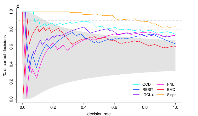
Figure 7: Accuracy decision-rates for the top baselines on the Tübingen Benchmark.

4 Conclusion

In this work, we develop a causal discovery method based on conditional quantiles. We propose bQCD, an effective implementation of our method based on nonparametric quantile regression, compares favorably to state-of-the-art methods on both simulated and real datasets. The new method should be preferred mainly because of three reasons. First, quantiles are less sensitive to outliers than the mean, thus bQCD is robust to contamination or heavy-tails, hence, it does not require preprocesing (“cleaning”) step. Second, we make no assumption on the parametric class considered, thus allowing for a wide range of mechanisms, whereas baselines perform worse when their assumptions are not satisfied. Third, our implementation is computationally more efficient than other nonparametric methods. There are currently three directions that we are explorig to extend this work. First, bQCD can be extended to multivariate cause-effect pairs. Second, it is interesting to see how quantile scores can fit in the invariant causal prediction framework (Peters et al., 2016). Third, the computational efficiency of bQCD is promising in the context of extensions to higher dimensional datasets. As such, ongoing research leverages existing graph discovery algorithms for hybrid learning, as suggested in the supplementary material. Fourth, as discussed in Remark 2, finding structural or distributional assumptions for which Assumption 1 or (11) holds remains an open problem.

Appendix A Theory

A.1 Proof of Theorem 2

We start by proving the sufficiency part of the theorem, namely that, if $\mbox{CL}(l)=o(n)$ for $l\in\{\tau,q_{X,\tau},q_{Y,\tau},q_{Y|X,\tau},q_{X|Y,\tau})\}$, then

$$P\left(\frac{\mbox{CL}_{\tau}(X)+\mbox{CL}_{\tau}(Y\mid X)}{\mbox{CL}_{\tau}(Y)+\mbox{CL}_{\tau}(X\mid Y)}\leq 1\right)\underset{n\to\infty}{\longrightarrow}1$$ (8)

implies that

$$\frac{\mathbb{E}\left[S_{\tau}(q_{X,\tau},X_{i})\right]+\mathbb{E}\left[S_{\tau}(q_{Y\mid X=X_{i},\tau},Y_{i})\right]}{\mathbb{E}\left[S_{\tau}(q_{Y,\tau},Y_{i})\right]+\mathbb{E}\left[S_{\tau}(q_{X\mid Y=Y_{i},\tau},X_{i})\right]}\leq 1.$$ (9)

First, notice that we have

$$\frac{\mbox{CL}_{\tau}(X)+\mbox{CL}_{\tau}(Y\mid X)}{\mbox{CL}_{\tau}(Y)+\mbox{CL}_{\tau}(X\mid Y)}=\frac{\sum\limits_{i=1}^{n}S_{\tau}(q_{X,\tau},X_{i})+\sum\limits_{i=1}^{n}S_{\tau}(q_{Y\mid X=X_{i},\tau},Y_{i})+K_{1}}{\sum\limits_{i=1}^{n}S_{\tau}(q_{Y,\tau},Y_{i})+\sum\limits_{i=1}^{n}S_{\tau}(q_{X\mid Y=Y_{i},\tau},X_{i})+K_{2}},$$ (10)

with

$$K_{1} =2\mbox{CL}(\tau)+\mbox{CL}(q_{X,\tau})+\mbox{CL}(q_{Y\mid X,\tau})-2a_{n}(\tau)=o(n)-2a_{n}(\tau),$$

$$K_{2} =2\mbox{CL}(\tau)+\mbox{CL}(q_{Y,\tau})+\mbox{CL}(q_{X\mid Y,\tau})-2a_{n}(\tau)=o(n)-2a_{n}(\tau).$$

Thus, we have that

$$\frac{\mbox{CL}_{\tau}(X)+\mbox{CL}_{\tau}(Y\mid X)}{\mbox{CL}_{\tau}(Y)+\mbox{CL}_{\tau}(X\mid Y)}\leq 1\iff\frac{\sum\limits_{i=1}^{n}S_{\tau}(q_{X,\tau},X_{i})+\sum\limits_{i=1}^{n}S_{\tau}(q_{Y\mid X=X_{i},\tau},Y_{i})}{\sum\limits_{i=1}^{n}S_{\tau}(q_{Y,\tau},Y_{i})+\sum\limits_{i=1}^{n}S_{\tau}(q_{X\mid Y=Y_{i},\tau},X_{i})}\leq 1+o_{p}(1),$$ (11)

where we used the fact that $K_{2}-K_{1}=o(n)$, which implies that

$$\frac{K_{2}-K_{1}}{\sum\limits_{i=1}^{n}S_{\tau}(q_{Y,\tau},Y_{i})+\sum\limits_{i=1}^{n}S_{\tau}(q_{X\mid Y=Y_{i},\tau},X_{i})}=o_{p}(1).$$

Finally, (9) follows because the law of large numbers along with the continuous mapping theorem imply

$$\left|\frac{\sum\limits_{i=1}^{n}S_{\tau}(q_{X,\tau},X_{i})+\sum\limits_{i=1}^{n}S_{\tau}(q_{Y\mid X=X_{i},\tau},Y_{i})}{\sum\limits_{i=1}^{n}S_{\tau}(q_{Y,\tau},Y_{i})+\sum\limits_{i=1}^{n}S_{\tau}(q_{X\mid Y=Y_{i},\tau},X_{i})}-\frac{\mathbb{E}\left[S_{\tau}(q_{X,\tau},X_{i})\right]+\mathbb{E}\left[S_{\tau}(q_{Y\mid X=X_{i},\tau},Y_{i})\right]}{\mathbb{E}\left[S_{\tau}(q_{Y,\tau},Y_{i})\right]+\mathbb{E}\left[S_{\tau}(q_{X\mid Y=Y_{i},\tau},X_{i})\right]}\right|=o_{p}(1).$$

To prove necessity, assume that

$$P\left(\frac{\mbox{CL}_{\tau}(Y)+\mbox{CL}_{\tau}(X\mid Y)}{\mbox{CL}_{\tau}(X)+\mbox{CL}_{\tau}(Y\mid X)}\leq 1\right)\underset{n\to\infty}{\longrightarrow}1.$$

By the sufficiency part of the proof, this implies that

$$\frac{\mathbb{E}\left[S_{\tau}(q_{X,\tau},X_{i})\right]+\mathbb{E}\left[S_{\tau}(q_{Y\mid X=X_{i},\tau},Y_{i})\right]}{\mathbb{E}\left[S_{\tau}(q_{Y,\tau},Y_{i})\right]+\mathbb{E}\left[S_{\tau}(q_{X\mid Y=Y_{i},\tau},X_{i})\right]}\geq 1.$$

which establishes necessity by contraposition. $\square$

A.2 Proof of Theorem 3

We start by proving the sufficiency part of the theorem, namely that, if Assumption 2 holds, then

$$P\left(\frac{\mbox{CL}_{\tau}(X)+\mbox{CL}_{\tau}(Y\mid X)}{\mbox{CL}_{\tau}(Y)+\mbox{CL}_{\tau}(X\mid Y)}\leq 1\right)\underset{n\to\infty}{\longrightarrow}1$$ (12)

implies that

$$P\left(\frac{S_{X,\tau}+S_{Y\mid X,\tau}}{S_{Y,\tau}+S_{X\mid Y,\tau}}\leq 1\right)\underset{n\to\infty}{\longrightarrow}1.$$ (13)

Denote by $\widehat{\mbox{CL}}_{\tau}(\cdot)$ the quantity corresponding to $\mbox{CL}_{\tau}(X)$ but replacing the population quantile by estimates, namely

$$\widehat{\mbox{CL}}_{\tau}(X) =\mbox{CL}(\tau)+\mbox{CL}(\widehat{q}_{X,\tau})+S_{X,\tau}-a_{n}(\tau),$$

$$\widehat{\mbox{CL}}_{\tau}(Y\mid X) =\mbox{CL}(\tau)+\mbox{CL}(\widehat{q}_{Y\mid X,\tau})+S_{X\mid Y,\tau}-a_{n}(\tau),$$

and similarly for $Y$ and $X\mid Y$. Hence, we have

$$\frac{\widehat{\mbox{CL}}_{\tau}(X)+\widehat{\mbox{CL}}_{\tau}(Y\mid X)}{\widehat{\mbox{CL}}_{\tau}(Y)+\widehat{\mbox{CL}}_{\tau}(X\mid Y)}=\frac{S_{X,\tau}+S_{Y\mid X,\tau}+K_{1}}{S_{Y,\tau}+S_{X\mid Y,\tau}+K_{2}},$$ (14)

with

$$K_{1} =2\mbox{CL}(\tau)+\mbox{CL}(\widehat{q}_{X,\tau})+\mbox{CL}(\widehat{q}_{Y\mid X,\tau})-2a_{n}(\tau),$$

$$K_{2} =2\mbox{CL}(\tau)+\mbox{CL}(\widehat{q}_{Y,\tau})+\mbox{CL}(\widehat{q}_{X\mid Y,\tau})-2a_{n}(\tau).$$

Consistency of the estimators (i.e., Assumption 2) along with the continuous mapping theorem implies

$$\left|\frac{\mbox{CL}_{\tau}(X)+\mbox{CL}_{\tau}(Y\mid X)}{\mbox{CL}_{\tau}(Y)+\mbox{CL}_{\tau}(X\mid Y)}-\frac{\widehat{\mbox{CL}}_{\tau}(X)+\widehat{\mbox{CL}}_{\tau}(Y\mid X)}{\widehat{\mbox{CL}}_{\tau}(Y)+\widehat{\mbox{CL}}_{\tau}(X\mid Y)}\right|=o_{p}(1)$$ (15)

Therefore, combining (12) and (15), we have that

$$P\left(\frac{\widehat{\mbox{CL}}_{\tau}(X)+\widehat{\mbox{CL}}_{\tau}(Y\mid X)}{\widehat{\mbox{CL}}_{\tau}(Y)+\widehat{\mbox{CL}}_{\tau}(X\mid Y)}\leq 1\right)\underset{n\to\infty}{\longrightarrow}1.$$ (16)

In turn, from (14), we have that

$$\frac{\widehat{\mbox{CL}}_{\tau}(X)+\widehat{\mbox{CL}}_{\tau}(Y\mid X)}{\widehat{\mbox{CL}}_{\tau}(Y)+\widehat{\mbox{CL}}_{\tau}(X\mid Y)}\leq 1\iff\frac{S_{X,\tau}+S_{Y\mid X,\tau}}{S_{Y,\tau}+S_{X\mid Y,\tau}}\leq 1+\frac{K_{2}-K_{1}}{S_{Y,\tau}+S_{X\mid Y,\tau}}=1+o_{p}(1),$$ (17)

where the last equality follows from assuming, without loss of generality, that $CL(\tau)=o(n)$, which implies that $K_{1}=o(n)-2a_{n}(\tau)$ and $K_{2}=o(n)-2a_{n}(\tau)$ and thus that $K_{2}-K_{1}=o(n)$. Finally, (13) follows from combining (16) and (17).

To prove necessity, assume that

$$P\left(\frac{\mbox{CL}_{\tau}(Y)+\mbox{CL}_{\tau}(X\mid Y)}{\mbox{CL}_{\tau}(X)+\mbox{CL}_{\tau}(Y\mid X)}\leq 1\right)\underset{n\to\infty}{\longrightarrow}1.$$

By the sufficiency part of the proof, this implies that

$$P\left(\frac{S_{X,\tau}+S_{Y\mid X,\tau}}{S_{Y,\tau}+S_{X\mid Y,\tau}}\geq 1\right)\underset{n\to\infty}{\longrightarrow}1.$$

which establishes necessity by contraposition. $\square$

Appendix B bQCD implementation

To leverage Theorem 3 and Decision rule 1 for causal discovery, we need a flexible model that yields computable expressions for all conditional quantiles. We show the efficiency of our method independent of the choice of underlying regressor through various implementations, namely copulas, quantile forests and neural networks.

Algorithm 1 bQCD algorithm

  Inputs:

• $\left\{X_{i},Y_{i}\right\}^{n}_{i=1}$, $n$ i.i.d. observations of the rvs $X$ and $Y$,

• $qr$, a quantile regression method,

• $m$, the number of quantiles levels (weights/nodes pairs to approximate the integral).

  1. Transform $X$ and $Y$ to standard normal.

  2. Compute the quadrature weights and nodes $\left\{w_{j},\tau_{j}\right\}_{j=1}^{m}$.

  3. Compute the conditional and marginal scores for $X\rightarrow Y$ (and similarly for $Y\rightarrow X$):

  for $j=1$ to $m$ do

     

• Use the empirical quantile to compute $\widehat{q}_{X,\tau_{j}}$ and $S_{X,\tau_{j}}=\sum_{i=1}^{n}S_{\tau_{j}}(\widehat{q}_{X,\tau_{j}},X_{i})$.

• Use the method $qr$ to compute $\widehat{q}_{X|Y,\tau_{j}}$ and $S_{Y\mid X,\tau_{j}}=\sum_{i=1}^{n}S_{\tau_{j}}(\widehat{q}_{Y\mid X=X_{i},\tau_{j}},Y_{i})$.

  end for

  4. Compute the scores $\widehat{S}_{\star}=\sum_{j=1}^{m}w_{j}S_{\star,\tau_{j}}$ for $\star\in\{X,Y,Y\mid X,X\mid Y\}$.

  5. Define $S_{X\to Y}=\widehat{S}_{X}+\widehat{S}_{Y|X}$ and $S_{Y\to X}=\widehat{S}_{Y}+\widehat{S}_{X|Y}$.

  if $S_{Y\to X}>S_{X\to Y}$ then

     Define the causal direction as $d=X\rightarrow Y$.

  else if $S_{Y\to X}<S_{X\to Y}$ then

     Define the causal direction as $d=Y\rightarrow X$.

  end if

  Define the confidence score as $C=-S_{X\to Y}+S_{Y\to X}$.

  Output: ($d$, $C$)

Nonparametric copulas

Copulas (i.e., multivariate distributions with uniform margins), represent an appealing alternative to compute conditional quantiles. In a nutshell, copulas make it possible to flexibly model the dependence structure between random variables while avoiding assumptions about the scales, functional forms, or other restrictions imposed when dealing with marginal distributions.

Following (Joe, 1996), copulas lead to a useful representation of the distributions of $Y|X$ and $X|Y$, namely $F_{Y|X}(x,y)=P(Y\leq y|X=x)=P(V\leq v|U=u)=\partial_{u}C(u,v)$ where $C$ is a copula, $\partial_{u}C(u,v)=\partial C(u,v)/\partial u$, $u=F_{X}(x)$, and $v=F_{Y}(y)$, and similarly $F_{X|Y}(x,y)=\partial_{v}C(u,v)$. This means that conditional distributions can be evaluated by taking partial derivatives of the copula function. The $\tau$-quantiles of $Y|X$ can then be written as $F^{-1}_{Y|X}(x,\tau)=F^{-1}_{Y}((\partial_{u}C)^{-1}(u,\tau))$ and similarly for $F^{-1}_{X|Y}(\tau,y)$, with inverse functions of the copula derivatives are with respect to $\tau$. Using the above equations, one can then compute all $\tau$-quantiles using the marginal distributions and the copula. To benefit from a fully nonparametric estimation, in practice we use nonparametric copulas (Geenens et al., 2017). We implemented Quantile Copula Causal Discovery (bQCD) using the R interface (R Core Team, 2017) interface to vinecopulib called rvinecopulib (Nagler & Vatter, 2018) and Gauss-Legendre quadrature from the package statmod (Smyth, 2005). We refer to Section B.1 for more details.

Quantile forest

Another nonparametric and consistent way of estimating conditional quantiles is via quantile regression forests. In contrast to random forests (Breiman, 2001), for each node in each tree, quantile regression forest keeps the value of all observations in this node, not just their mean, which allows us to assess the conditional distribution based on this information. For detailed explanation of the algorithm and its consistency we refer the reader to the original paper (Meinshausen, 2006). In experiments we used nodesize=10, sampsize=50 and n_trees=500 for both regression directions.

Quantile neural network

Recently, quantile estimation has become of interest in the deep learning community as part of uncertainty estimation framework. We leverage such an approach for a flexible approximation of the conditional quantiles which are estimated simultaneously by a neural network trained with pinball loss, i.e. the quantile scoring as a loss function. In the experiments we use the qrnn package by Cannon (2018) which includes monotonicity constraints to guard against quantile crossing. Again, for both sides (possible causal directions) we use symmetric models, which is a two-layered neural network with 10 neurons per layer, with sigmoid nonlinearities. The networks were trained to 1000 iterations.

B.1 Predicting Quantiles with Copulas

While not the only statistical model satisfying Assumption 2, copulas (i.e., multivariate distributions with uniform margins), represent an appealing alternative. Any bivariate nonparametric estimator allowing to compute the required inverse conditional CDFs could be used. But, to the best of our knowledge, no available implementation allows directly for this. With copulas, obtaining conditional quantiles is straightforward through (18). And they are implemented efficiently because they appear in higher-dimensional models such as vines (Bedford et al., 2002; Aas et al., 2009).

According to the theorem of (Sklar, 1959), any $F$ can be represented by its marginal distributions $F_{X},F_{Y}$ and a copula $C$, which is is the joint distribution of $(U,V)=\bigl{(}F_{X}(X),F_{Y}(Y)\bigr{)}$. In other words, for any $F$, there exists a $C$ such that $F(x,y)=C(F_{X}(x),F_{Y}(y))$ for each $(x,y)\in{\mathbb{R}}^{2}$. Moreover, if all the distributions are continuous, then $C$ is unique.

Following (Joe, 1996), copulas lead to a useful representation of the distributions of $Y|X$ and $X|Y$, namely $F_{Y|X}(x,y)=P(Y\leq y|X=x)=P(V\leq v|U=u)=\partial_{u}C(u,v)$ where $\partial_{u}C(u,v)=\partial C(u,v)/\partial u$, $u=F_{X}(x)$, and $v=F_{Y}(y)$, and similarly $F_{X|Y}(x,y)=\partial_{v}C(u,v)$. This means that conditional distributions can be evaluated by taking partial derivatives of the copula function. The $\tau$-quantiles of $Y|X$ can then be written as

$$F^{-1}_{Y|X}(x,\tau)=F^{-1}_{Y}((\partial_{u}C)^{-1}(u,\tau)),$$ (18)

and similarly for $F^{-1}_{X|Y}(\tau,y)$, with inverse functions of the copula derivatives are with respect to $\tau$. Using (18), one can then compute all $\tau$-quantiles using the marginal distributions and the copula.

Assume that we have $n$ i.i.d. random variables $\left\{(X_{1},Y_{1}),\cdots,(X_{n},Y_{n})\right\}$. To avoid relying on restrictive assumptions, $S_{X\to Y}$ and $S_{Y\to X}$ are estimated completely nonparametrically.

Note that, if all the considered distributions are differentiable, $F(x,y)=C(F_{X}(x),F_{Y}(y))$ implies

$$f(x,y)=c\bigl{\{}F_{X}(x),F_{Y}(y)\bigr{\}}f_{X}(x)f_{Y}(x),$$ (19)

where $f,c,f_{X}$, and $f_{Y}$ are the densities corresponding to $F,C,F_{X}$, and $F_{Y}$ respectively. Equation (19) has an important implication for inference: because the right-hand side is a product, the joint log-likelihood can be written as a sum of the log-likelihood of each margin and the log-likelihood of the copula. This fact can be conveniently exploited in a two-step procedure: estimate the margins separately to obtain $\widehat{F}_{X}$ and $\widehat{F}_{Y}$, and then take the probability integral transform of the data using those margins, that is, define $\widehat{U}_{i}=\widehat{F}_{X}(X_{i})$ and $\widehat{V}_{i}=\widehat{F}_{Y}(Y_{i})$, to estimate $\widehat{C}$.

For the first step, we simply use the empirical distribution $\widehat{F}_{X}(x)=\sum_{i=1}^{n}\mathbb{I}\left\{X_{i}\leq x\right\}/(n+1)$ (and similarly for $Y$), where $n+1$ is used instead of $n$ in the copula context to avoid boundary problems. Discrete datasets are handled by jittering, that is breaking ties at random. As for the second step, since typical nonparametric estimators are targeted at densities with unbounded support, they are unsuited to densities restricted to $[0,1]^{2}$. To get around this issue, (Scaillet et al., 2007) suggests to first transform the data to standard normal margins, and then use any nonparametric estimator suited to unbounded densities. The transformation estimator of the copula density $c(u,v)$ is then defined as

$$\widehat{c}(u,v)=\frac{\widehat{g}(\Phi^{-1}(u)-\Phi^{-1}(\widehat{U}_{i}),\Phi^{-1}(v)-\Phi^{-1}(\widehat{V}_{i}))}{\phi(\Phi^{-1}(u))\phi(\Phi^{-1}(v))},$$ (20)

where $\widehat{U}_{i}=\widehat{F}_{X}(X_{i})$, $\widehat{V}_{i}=\widehat{F}_{Y}(Y_{i})$, $\widehat{g}$ is a bivariate nonparametric estimator, and $\phi,\Phi$ denote the standard normal density and distribution, respectively. Following (Scaillet et al., 2007; Geenens et al., 2017), we then use a bivariate Gaussian kernel estimator for $\widehat{g}$.

The consistency and asymptotic normality of this estimator are derived in (Geenens et al., 2017). Given that the empirical distribution is also consistent, consistency of the resulting joint distribution is also straightforward. Furthermore, using the fact that $F_{X}(x)=F(x,\infty)$, $F_{Y}(y)=F(\infty,y)$, $F_{X|Y}(x,y)=\partial_{y}F(x,y)/\left.\partial_{y}F(x,y)\right|_{x\to\infty}$, $F_{Y|X}(x,y)=\partial_{x}F(x,y)/\left.\partial_{x}F(x,y)\right|_{y\to\infty}$, consistent estimators of the marginal and conditional distributions are obtained by replacing $F$ by the copula-based joint estimator and using the same relations.

The transformation kernel estimator for bivariate copula densities is implemented in C++ as part of vinecopulib (Nagler & Vatter, 2017), a header-only C++ library for copula models based on Eigen (*)eigenweb and Boost (Schäling, 2011). From (20), vinecopulib constructs and stores a $30\times 30$ grid over $[0,1]^{2}$ along with the evaluated density at the grid points. Then, a cubic-spline approximation makes it possible to efficiently compute the copula distribution $\widehat{C}(u,v)$ and its derivatives, $\partial_{u}\widehat{C}(u,v)$ and $\partial_{v}\widehat{C}(u,v)$, as the integrals of the spline-approximation of the density admits an analytic expression. Finally, vinecopulib implements the numerical inversion of $\partial_{u}\widehat{C}(u,v)$ and $\partial_{v}\widehat{C}(u,v)$ to compute $(\partial_{u}\widehat{C})^{-1}(u,v)$ and $(\partial_{v}\widehat{C})^{-1}(u,v)$ by a vectorized version of the bisection method.

Appendix C Baseline implementation details

C.1 Baselines - Implementations and hyper parameters

For IGCI, we use the original implementation of Janzing et al. (2012) with slope-based estimation with both gaussian and uniform reference measure. For LINGAM, we use the implementation of Peters et al. (2014), which also provides RESIT with GP regression and the HSIC independence test with a threshold value $\alpha=0.05$. For CAM, we use the R package (Peters & Ernest, 2015) with the default parameters. For GR-AN and EMD, we use the code of Hernández-Lobato et al. (2016). The parameters for EMD on simulated data are as in the original paper, $\lambda=1e^{-3}$ and $\sigma=\frac{1}{5}S_{m}$ ($S_{m}$ being the median of distances across all input patterns). For the real data benchmark, GR-AN was evaluated over 15 subsamples limited to 500 observations, and the results are then averaged. However, the parameters are tuned and selected from the overall best results. GR-AN has a built-in function that takes care parameter tuning.

For Slope, we use the implementation of Marx & Vreeken (2017), with local regression included in the fitting process. For PNL, GPI-MML, and ANM, we use the MATLAB implementation from the Cause Effect Pairs Challenge FirfiD, with the same setup as RESIT for ANM. For Sloppy we use the results as provided with the code of (Marx & Vreeken, 2019) with the AIC score. For RECI we use an example MATLAB code provided by the authors with the ’log’ implementation, with and without the data preprocessing step. Because there is no publicly available implementation of CURE, we use the results from files obtained by Marx & Vreeken (2017). Our code and datasets used for the paper are included in the submitted supplementary package.

All experiments are carried out using R version 3.4.1 on a MacBook Pro (mid-2015) with 16GB memory, a 2.2 GHz Intel Core i7 processor and 250GB SSD.

C.2 Computational complexity

Figure 9: Linear scaling of bQCD over 100 pairs, $m=1$, $n$ varies

Appendix D Additional results from experiments

D.1 Tabular results for spider plots

Table 2: Accuracy on simulated and real data.

	SIM	SIM-c	SIM-ln	SIM-G	AN	AN-s	LS	LS-s	MN-U	Tüb	Tüb weigh.
bQCD m = 1	0.57	0.69	0.69	0.59	0.99	0.47	1	0.93	0.23	0.64	0.74
bQCD m = 3	0.61	0.72	0.76	0.65	1	0.81	1	0.98	0.99	0.69	0.77
bQCD m = 7	0.65	0.76	0.74	0.66	1	0.82	1	0.98	0.99	0.67	0.75
IGCI - u	0.42	0.49	0.52	0.54	0.41	0.27	0.63	0.37	0.07	0.67	0.72
IGCI - g	0.36	0.46	0.62	0.85	0.98	0.98	0.99	0.94	0.74	0.61	0.64
biCAM	0.57	0.6	0.87	0.81	1	1	1	0.53	0.86	0.57	0.58
Slope	0.45	0.54	0.47	0.48	0.18	0.18	0.21	0.17	0.07	0.75	0.83
RESIT	0.78	0.82	0.87	0.77	1	1	0.6	0.03	0.05	0.53	0.63
ANM	0.76	0.81	0.80	0.77	1	1	0.62	0.09	0.03	0.59	0.59
LINGAM	0.42	0.53	0.31	0.25	0	0.04	0.07	0.03	0	0.27	0.42
EMD	0.45	0.4	0.52	0.58	0.36	0.33	0.6	0.42	0.83	0.6	0.68
GRAN	0.48	0.44	0.43	0.37	0.05	0.06	0.11	0.20	0.5	0.4	0.5
GPI	0.82	0.86	0.88	0.94	0.95	0.11	0.91	0.54	0.90	0.6	0.63
PNL	0.70	0.65	0.61	0.64	0.96	0.63	0.91	0.44	0.66	0.75	0.73
Sloppy	0.64	0.62	0.77	0.81	1	1	1	0.56	0.96,	0.59	0.74
RECI w/wo pp	0.7/0.6	0.71/0.65	0.8/0.71	0.66/0.67	0.72/0.72	0.15/0.17	0.82/0.67	0.71/0.52	0.88/0.88	0.61/0.63	0.7/0.67

Table 3: Accuracy on simulated and real data for different selection of $\tau$ values.

	SIM	SIM-c	SIM-ln	SIM-G	AN	AN-s	LS	LS-s	MN-U	Tueb	Tueb-w
$\tau\in[0.1,0.5,0.9]$	0.61	0.72	0.76	0.65	1	0.81	1	0.98	0.99	0.69	0.77
$\tau\in[0.4,0.5,0.6]$	0.56	0.71	0.72	0.58	1	0.45	1	0.95	0.25	0.63	0.73

Table 4: Area under the ROC and PR curves for bQCD.

	SIM	SIM-c	SIM-ln	SIM-G	AN	AN-s	LS	LS-s	MN-U
ROC-AUC	0.67	0.79	0.87	0.69	1	0.9	1	1	1
PR-AUC	0.67	0.82	0.86	0.7	1	0.89	1	1	1

Note that due to RESIT being undecided in few of the real data pairs, we observe the random classifier behavior at the beginning of its ROC curve in Figure 10.

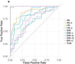
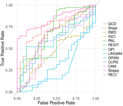
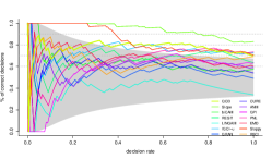
Figure 10: ROC curves (a) for bQCD all benchmarks, (b) all baselines on Tuebingen, (c) and weighted accuracy-decision rate curves for all baselines on the Tübingen dataset.

Appendix E Extensions of the pairwise method

Recent work by Goudet et al. (2017a) suggests that pairwise and CPDAG (i.e., the skeleton and the $v$-structures) learning procedures can suitably complement each other. In this section, we follow a similar approach to suggest an extension of bQCD to multivariate datasets: start from the CPDAG resulting from another method, and then use bQCD to orient the edges. We rank edges and include them in the graph sequentially, starting from the edge with the highest confidence, while checking the acyclicity of the resulting graph after each addition. Note that this approach also requires a final verification to test edge orientation and $v$-structures consistency (Goudet et al., 2017a).

We do this by using CAM to learn a CPDAG and then use bQCD to orient its edges. The rationale is that, while Bühlmann et al. (2014) proves the consistency of the variable ordering by CAM used to learn the structure even when its assumptions are not met, bQCD is better in pairwise discoveries (see Section 3). But we could also have used the PC algorithm (Spirtes et al., 2000b).

We now turn to the well know protein causal dataset by Sachs et al. (2005), for which a ground truth DAG of the causal structure is provided. We used the cd3cd28 dataset with 853 observations of 11 proteins. For evaluation we use the structural hamming distance (SHD) as proposed in (Tsamardinos et al., 2006) (adding, removing or reversing an edge) necessary to transform one graph to the another and the structural intervention distance (SID), as in (Pet, 2015), which is considered to be appropriate for quantifying the correct order among variables, by estimating the causal effects they entail. CAM by itself outputs a DAG with $SID_{CAM}=53$, and $SHD_{CAM}=17$, while with bQCD we can reduce this to average $SID_{bQCD}=46(2.5)$, and average $SHD_{bQCD}=15.1(1.6)$. In Table 5 we provide the average results over ten random sub-samples of the dataset where the edges of CAM’s CPDAG were oriented by each of the pairwise methods . From the presented results, we note that bQCD achieves best scores in terms of SHD and SID.

So What exactly is the nature of the output on these undirected/directed edges, are there reported confidence scores on why the edge wasn’t oriented e.g. if it were borderline or not

As such, it is reassuring that bQCD is able to correctly decide for the causal direction, even though other dependencies affect the pairwise (direct) causal relationships in such confounded dataset. While such results are promising, a consistent hybrid method extending bQCD and quantile based methods to higher dimensional datasets is left for further work. Even in this simplified setting, if one were to use Decision rule 1 on all pairwise adjacent vertices in a CPDAG, one may still get a PDAG (i.e., due to non-decisions). Furthermore, extensions to higher dimensional settings could use quantile based independence tests in RESIT, or replace mean regression in CAM by quantile regression.

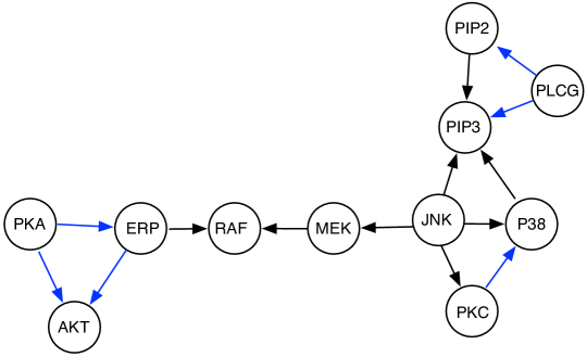
Figure 11: Causal protein network as obtained by CAM’s CPDAG oriented with bQCD. Blue edges are correctly oriented.

Table 5: SID and SHD for the Sachs dataset using CAM CPDAG with causal directions from pairwise methods by 10-fold cross validation. Average and standard deviations.

	bQCD	IGCI-u	Slope	RESIT	CAM	EMD	LINGAM	GRAN	Random
SID	46.5(2.5)	50.3(1.9)	54.5(3.3)	51(0)	53.4(1.4)	51.5(2.7)	48.9(0.87)	49.5(4)	52.5(3.6)
SHD	15.1(1.6)	15.8(1.7)	17.6(1.2)	14(0.3)	15.4(1.6)	16(1.7)	14.3(0.82)	16.4(1.34)	17.2(1.4)

Appendix F Scatter plots of simulated pairs

Figure 12: SIM/SIM-ln/SIM-G (first/second/third row).

Figure 13: By row AN/AN-s/LS/LS-s/MN.

References

- Pea (2010) An Introduction to Causal Inference. The International Journal of Biostatistics, 2010.
- Voo (2014) Graph estimation with joint additive models. Biometrika, 2014.
- Pet (2015) Structural Intervention Distance for Evaluating Causal Graphs. Neural Computation, 27(3):771–799, mar 2015.
- Aas et al. (2009) Aas, K., Czado, C., Frigessi, A., and Bakken, H. Pair-copula constructions of multiple dependence. Insurance: Mathematics and economics, 44(2):182–198, 2009.
- Aue et al. (2014) Aue, A., Cheung, R. C. Y., Lee, T. C. M., and Zhong, M. Segmented model selection in quantile regression using the minimum description length principle. Journal of the American Statistical Association, 109(109):507–1241, 2014.
- Bauer & Czado (2016a) Bauer, A. and Czado, C. Pair-copula Bayesian networks. Journal of Computational and Graphical Statistics, 25(4):1248–1271, 2016a.
- Bauer & Czado (2016b) Bauer, A. and Czado, C. Pair-copula Bayesian networks. Journal of Computational and Graphical Statistics, 25(4):1248–1271, 2016b.
- Bauer et al. (2012) Bauer, A., Czado, C., and Klein, T. Pair-copula constructions for non-Gaussian DAG models. The Canadian Journal of Statistics, 40(1):86–109, 2012.
- Bedford et al. (2002) Bedford, T., Cooke, R. M., et al. Vines–a new graphical model for dependent random variables. The Annals of Statistics, 30(4):1031–1068, 2002.
- Besag (1974) Besag, J. Spatial Interaction and the Statistical Analysis of Lattice Systems. Journal of the Royal Statistical Society. Series B (Methodological), 36(2):192–236, 1974.
- Blöbaum et al. (2018) Blöbaum, P., Janzing, D., Washio, T., Shimizu, S., and Schölkopf, B. Cause-effect inference by comparing regression errors. In International Conference on Artificial Intelligence and Statistics, pp. 900–909, 2018.
- Breiman (2001) Breiman, L. Random forests. Machine learning, 45(1):5–32, 2001.
- (13) Budhathoki, K. and Vreeken, J. MDL for Causal Inference on Discrete Data.
- Budhathoki & Vreeken (2017) Budhathoki, K. and Vreeken, J. Causal inference by compression. In ICDM, pp. 41–50, 2017.
- Bühlmann et al. (2014) Bühlmann, P., Peters, J., and Ernest, J. CAM: Causal additive models, high-dimensional order search and penalized regression. Annals of Statistics, 42(6):2526–2556, 2014.
- Cannon (2018) Cannon, A. J. Non-crossing nonlinear regression quantiles by monotone composite quantile regression neural network, with application to rainfall extremes. Stochastic Environmental Research and Risk Assessment, pp. 3207–3225, 2018. ISSN 1436-3259.
- Chalupka et al. (2017) Chalupka, K., Eberhardt, F., and Perona, P. Causal feature learning: an overview. Behaviormetrika, 44(1):137–164, 2017.
- Chang et al. (2016) Chang, Y., Li, Y., Ding, A., and Dy, J. A robust-equitable copula dependence measure for feature selection. AISTATS, 41:84–92, 2016.
- Chen et al. (2014) Chen, Z., Zhang, K., Chan, L., and Schölkopf, B. Causal discovery via reproducing kernel hilbert space embeddings. Neural Computation, 26(7):1484–1517, 2014.
- Chickering (2002) Chickering, D. M. Optimal Structure Identification With Greedy Search. Journal of Machine Learning Research, 3:507–554, 2002.
- Cui et al. (2016) Cui, R., Groot, P., and Heskes, T. Copula PC algorithm for causal discovery from mixed data. In Lecture Notes in Computer Science (including subseries Lecture Notes in Artificial Intelligence and Lecture Notes in Bioinformatics), volume 9852 LNAI, pp. 337–392. Springer, Cham, sep 2016.
- Dawid et al. (2007) Dawid, C. A. et al. Fundamentals of statistical causality. 2007.
- Drton & Maathuis (2017) Drton, M. and Maathuis, M. H. Structure Learning in Graphical Modeling. Annual Review of Statistics and Its Application, 4:365–393, 2017.
- Elidan (2010) Elidan, G. Copula Bayesian Networks. In NIPS 23, pp. 559–567, 2010.
- Elidan (2013) Elidan, G. Copulas in machine learning. In Copulae in mathematical and quantitative finance, pp. 39–60. Springer, 2013.
- Embrechts et al. (1999) Embrechts, P., Mcneil, E., and Straumann, D. Correlation: Pitfalls and alternatives. Risk Magazine, 1999.
- Ernest (2016) Ernest, J. Causal inference in semiparametric and nonparametric structural equation models ETH Library. PhD thesis, 2016.
- (28) Fisher, R. A. Statistical Methods for Research Workers.
- Fisher (1936) Fisher, R. A. Statistical methods for research workers. Especially Section, 21, 1936.
- Flaxman et al. (2016) Flaxman, S. R., Neill, D. B., and Smola, A. J. Gaussian Processes for Independence Tests with Non-iid Data in Causal Inference. ACM Transactions on Intelligent Systems and Technology (TIST), 7(2):21–22, 2016.
- Freedman & Diaconis (1981) Freedman, D. and Diaconis, P. On the histogram as a density estimator:l2 theory. Zeitschrift für Wahrscheinlichkeitstheorie und Verwandte Gebiete, 57(4):453–476, Dec 1981. ISSN 1432-2064. doi: 10.1007/BF01025868. URL https://doi.org/10.1007/BF01025868.
- Geenens et al. (2017) Geenens, G., Charpentier, A., and Paindaveine, D. Probit transformation for nonparametric kernel estimation of the copula density. Bernoulli, 23(3):1848–1873, 2017.
- Geraci & Bottai (2007) Geraci, M. and Bottai, M. Quantile regression for longitudinal data using the asymmetric laplace distribution. Biostatistics, 8(1):140–154, 2007.
- Gneiting (2011) Gneiting, T. Making and evaluating point forecasts. Journal of the American Statistical Association, 106(494):746–762, jun 2011.
- Goudet et al. (2017a) Goudet, O., Kalainathan, D., Caillou, P., Guyon, I., Lopez-Paz, D., and Sebag, M. Causal Generative Neural Networks. 2017a.
- Goudet et al. (2017b) Goudet, O., Kalainathan, D., Caillou, P., Lopez-Paz, D., Guyon, I., Sebag, M., Tritas, A., and Tubaro, P. Learning functional causal models with generative neural networks. preprint, nov 2017b. arXiv: 1709.05321.
- Grünwald & Grunwald (2007) Grünwald, P. D. and Grunwald, A. The minimum description length principle. MIT press, 2007.
- Guennebaud et al. (2010) Guennebaud, G., Jacob, B., and Others. Eigen v3, 2010. URL http://eigen.tuxfamily.org.
- Hall & Hannan (1988) Hall, P. and Hannan, E. J. On stochastic complexity and nonparametric density estimation. Biometrika, 75(4):705–714, 1988.
- Hansen & Yu (2001) Hansen, M. H. and Yu, B. Model selection and the principle of minimum description length. Journal of the American Statistical Association, 96(454):746–774, 2001.
- Harrell Jr et al. (2017) Harrell Jr, F. E., with contributions from Charles Dupont, and others., M. Hmisc: Harrell Miscellaneous, 2017. URL https://cran.r-project.org/package=Hmisc.
- Harris & Drton (2013) Harris, N. and Drton, M. PC Algorithm for nonparanormal graphical models. Journal of Machine Learning Research, 14:3365–3383, 2013.
- Heinze-Deml et al. (2018) Heinze-Deml, C., Peters, J., and Meinshausen, N. Invariant causal prediction for nonlinear models. Journal of Causal Inference, 6(2), 2018.
- Hernández-Lobato et al. (2016) Hernández-Lobato, D., Morales Mombiela, P., Lopez-Paz, D., and Suárez, A. Non-linear causal inference using Gaussianity measures. Journal of Machine Learning Research, 17(1):939–977, 2016.
- Hernández-Orallo & Dowe (2010) Hernández-Orallo, J. and Dowe, D. L. Measuring universal intelligence: Towards an anytime intelligence test. Artificial Intelligence, 174(18):1508–1539, 2010.
- Hoeffding (1948) Hoeffding, W. A Non-Parametric Test of Independence. The Annals of Mathematical Statistics, 19(4):546–557, 1948.
- Hoyer et al. (2009) Hoyer, P. O., Janzing, D., Mooij, J., Peters, J., and Schölkopf, B. Nonlinear causal discovery with additive noise models. In NIPS 22, pp. 689–696, 2009.
- Hyvärinen & Smith (2013) Hyvärinen , A. and Smith, S. M. Pairwise Likelihood Ratios for Estimation of Non-Gaussian Structural Equation Models. Journal of Machine Learning Research, 14:111–152, 2013.
- Janzing & Schölkopf (2010) Janzing, D. and Schölkopf, B. Causal Inference using the algorithmic markov condition. IEEE Transactions on Information Theory, 56(10):5168–5194, 2010.
- (50) Janzing, D., Peters, J., Mooij, J., and Schölkopf, B. Identifying confounders using additive noise models.
- Janzing et al. (2012) Janzing, D., Mooij, J., Zhang, K., Lemeire, J., Zscheischler, J., Daniušis, P., Steudel, B., and Schölkopf, B. Information-geometric approach to inferring causal directions. Artificial Intelligence, 182:1–31, 2012.
- Joe (1996) Joe, H. Families of m-variate distributions with given margins and m(m-1)/2 bivariate dependence parameters. In Distributions with fixed marginals and related topics, pp. 120–141. Institute of Mathematical Statistics, 1996.
- Karra & Mili (2016) Karra, K. and Mili, L. Hybrid Copula Bayesian Networks. In Conference on Probabilistic Graphical Models, volume 52, pp. 240–251, 2016.
- Kocaoglu et al. (2017) Kocaoglu, M., Dimakis, A. G., Vishwanath, S., and Hassibi, B. Entropic causal inference. In Thirty-First AAAI Conference on Artificial Intelligence, 2017.
- Koenker & Machado (1999) Koenker, R. and Machado, J. A. Goodness of fit and related inference processes for quantile regression. Journal of the american statistical association, 94(448):1296–1310, 1999.
- Koenker, Roger (2005) Koenker, Roger . Quantile regression. Econometric Society monographs, 2005.
- Kolmogorov (1963) Kolmogorov, A. N. On tables of random numbers. Sankhyā: The Indian Journal of Statistics, Series A, pp. 369–376, 1963.
- Kpotufe et al. (2014) Kpotufe, S., Sgouritsa, E., Janzing, D., and Schölkopf, B. Consistency of causal inference under the additive noise model. In ICML 31, pp. 478–486, 2014.
- Lichman (2013) Lichman, M. {UCI} Machine Learning Repository, 2013. URL http://archive.ics.uci.edu/ml.
- Liu & Chan (2017) Liu, F. and Chan, L.-W. Causal inference on multidimensional data using free probability theory. IEEE Transactions on Neural Networks and Learning Systems, 2017.
- Liu et al. (2009) Liu, H., Lafferty, J., and Wasserman, L. The Nonparanormal: semiparametric estimation of high dimensional undirected graphs. Journal of Machine Learning Research, 10:2295–2328, 2009.
- Loader (2006) Loader, C. Local regression and likelihood. Springer Science & Business Media, 2006.
- Lopez-Paz (2016) Lopez-Paz, D. From Dependence to Causation. PhD thesis, University of Cambridge, 2016.
- Lopez-Paz et al. (2013) Lopez-Paz, D., Hernandez-Lobato, J. M., and Schölkopf, B. Semi-supervised domain adaptation with copulas. NIPS 26, pp. 674–682, 2013.
- Lopez-Paz et al. (2015) Lopez-Paz, D., Muandet, K., Schölkopf, B., and Tolstikhin, I. Towards a learning theory of cause-effect inference. In ICML 32, pp. 1452–1461, 2015.
- Maathuis & Nandy (2016) Maathuis, M. H. and Nandy, P. A review of some recent advances in causal inference. In Handbook of Big Data. CRC Press, 2016.
- Mandros et al. (2017) Mandros, P., Boley, M., and Vreeken, J. Discovering reliable approximate functional dependencies. KDD, pp. 355–364, 2017.
- Marx & Vreeken (2017) Marx, A. and Vreeken, J. Telling cause from effect using MDL-based local and global regression. In ICDM, 2017.
- Marx & Vreeken (2019) Marx, A. and Vreeken, J. Identifiability of cause and effect using regularized regression. In ACM SIGKDD, 2019.
- Meinshausen (2006) Meinshausen, N. Quantile regression forests. JMLR, 2006.
- Mitrovic et al. (2018) Mitrovic, J., Sejdinovic, D., and Teh, Y. W. Causal inference via kernel deviance measures. In Advances in Neural Information Processing Systems, pp. 6986–6994, 2018.
- Mooij et al. (2009) Mooij, J., Janzing, D., Peters, J., and Schölkopf, B. Regression by dependence minimization and its application to causal inference in additive noise models. In ICML 26, pp. 745–752, 2009.
- Mooij et al. (2010) Mooij, J. M., Stegle, O., Janzing, D., Zhang, K., and Schölkopf, B. Probabilistic latent variable models for distinguishing between cause and effect. In NIPS 23, pp. 1687–1695, 2010.
- Mooij et al. (2016) Mooij, J. M., Peters, J., Janzing, D., Zscheischler, J., and Schölkopf, B. Distinguishing cause from effect using observational data: methods and benchmarks. Journal of Machine Learning Research, 17:1–102, 2016.
- Müller & Czado (2017) Müller, D. and Czado, C. Selection of sparse vine copulas in high dimensions with the lasso. may 2017.
- Nagler & Vatter (2017) Nagler, T. and Vatter, T. vinecopulib: High Performance Algorithms for Vine Copula Modeling in C++. http://vinecopulib.org, 2017.
- Nagler & Vatter (2018) Nagler, T. and Vatter, T. rvinecopulib: high performance algorithms for vine copula modeling, 2018. URL https://cran.r-project.org/package=rvinecopulib.
- Oates et al. (2016a) Oates, C. J., Smith, J. Q., and Mukherjee, S. Estimating Causal Structure Using Conditional DAG Models. Journal of Machine Learning Research, 17:1–23, 2016a.
- Oates et al. (2016b) Oates, C. J., Smith, J. Q., and Mukherjee, S. Estimating Causal Structure Using Conditional DAG Models. Journal of Machine Learning Research, 17:1–23, 2016b.
- Pearl (1988) Pearl, J. Probabilistic Reasoning in Intelligent Systems: Networks of Plausible Inference. Morgan Kaufmann Series in Representation and Reasoning, 1988.
- Pearl (2009) Pearl, J. Causality. Cambridge University Press, 2009.
- Pearl et al. (2016) Pearl, J., Glymour, M., and Jewell, N. P. Causal Inference in Statistics: A Primer. John Wiley & Sons, 2016.
- Peters & Ernest (2015) Peters, J. and Ernest, J. CAM: Causal Additive Model (CAM), 2015. URL https://cran.r-project.org/package=CAM.
- Peters et al. (2011) Peters, J., Mooij, J. M., Janzing, D., and Schölkopf, B. Identifiability of causal graphs using functional models. In UAI 27, pp. 589–598, 2011.
- Peters et al. (2014) Peters, J., Mooij, J. M., Janzing, D., and Schölkopf, B. Causal discovery with continuous additive noise models. Journal of Machine Learning Research, 15(1):2009–2053, 2014.
- Peters et al. (2016) Peters, J., Bühlmann, P., and Meinshausen, N. Causal inference by using invariant prediction: identification and confidence intervals. Journal of the Royal Statistical Society. Series B: Statistical Methodology, 78(5):947–1012, 2016.
- Peters et al. (2017) Peters, J., Janzing, D., and Schölkopf, B. Elements of Causal Inference: Foundations and Learning Algorithms. MIT Press (available on-line), 2017.
- Pircalabelu et al. (2017) Pircalabelu, E., Claeskens, G., and Gijbels, I. Copula directed acyclic graphs. Statistics and Computing, 27(1):55–78, 2017.
- R Core Team (2017) R Core Team. R: A language and environment for statistical computing, 2017. URL https://www.r-project.org/.
- Rasmussen & Williams (2006) Rasmussen, C. E. and Williams, C. K. I. Gaussian Processes for Machine Learning, volume 1. MIT Press Cambridge, 2006.
- Rissanen (1978) Rissanen, J. Modeling by shortest data description. Automatica, 14(5):465–471, 1978.
- Rissanen (1983) Rissanen, J. A Universal Prior for Integers and Estimation by Minimum Description Length. The Annals of Statistics, 11(2):416–431, 1983.
- Rissanen (1986) Rissanen, J. Stochastic complexity and modeling. The annals of statistics, pp. 1080–1100, 1986.
- Rissanen (2005) Rissanen, J. Complexity and Information in Modeling. pp. 1–16, 2005.
- Rissanen et al. (1992) Rissanen, J., Speed, T. P., and Yu, B. Density estimation by stochastic complexity. IEEE Transactions on Information Theory, 38(2):315–323, 1992.
- Rojas-Carulla et al. (2017) Rojas-Carulla, M., Baroni, M., and Lopez-Paz, D. Causal Discovery Using Proxy Variables. 2017.
- Sachs et al. (2005) Sachs, K., Perez, O., Pe’er, D., Lauffenburger, D. A., and Nolan, G. P. Causal Protein-Signaling Networks Derived from Multiparameter Single-Cell Data. Science, 308(5721):523–529, apr 2005.
- Scaillet et al. (2007) Scaillet, O., Charpentier, A., and Fermanian, J.-D. The estimation of copulas: Theory and practice. Technical report, Ensae-Crest and Katholieke Universiteit Leuven, NP-Paribas and Crest; HEC Genève and Swiss Finance Institute, 2007.
- Schäling (2011) Schäling, B. The Boost C++ Libraries. 2011.
- Schölkopf (2019) Schölkopf, B. Causality for machine learning. arXiv preprint arXiv:1911.10500, 2019.
- Schölkopf et al. (2012) Schölkopf, B., Janzing, D., Peters, J., Sgouritsa, E., Zhang, K., and Mooij, J. On causal and anticausal learning. In ICML 29, pp. 1255–1262, 2012.
- Schölkopf et al. (2016) Schölkopf, B., Hogg, D. W., Wang, D., Foreman-Mackey, D., Janzing, D., Simon-Gabriel, C.-J., and Peters, J. Modeling confounding by half-sibling regression. Proceedings of the National Academy of Sciences, 2016.
- Sgouritsa et al. (2015) Sgouritsa, E., Janzing, D., Hennig, P., and Schölkopf, B. Inference of cause and effect with unsupervised inverse regression. In AISTATS 38, pp. 847–855, 2015.
- Shimizu et al. (2006) Shimizu, S., Hoyer, P., Hyvärinen , Aapo, and Antti, K. A linear non-gaussian acyclic model for causal discovery. Journal of Machine Learning Research, 7:2003–2030, 2006.
- Sklar (1959) Sklar, A. Fonctions de répartition à n dimensions et leurs marges. Publications de L’Institut de Statistique de L’Université de Paris, 8:229–231, 1959.
- Smyth (2005) Smyth, G. K. Numerical integration. Encyclopedia of Biostatistics, pp. 3088–3095, 2005.
- Spirtes & Glymour (1991) Spirtes, P. and Glymour, C. An algorithm for fast recovery of sparse causal graphs. Social science computer review, 9(1):62–72, 1991.
- Spirtes & Zhang (2016) Spirtes, P. and Zhang, K. Causal discovery and inference: Concepts and recent methodological advances. Applied Informatics, pp. 165–191, 2016.
- Spirtes et al. (1995) Spirtes, P., Meek, C., and Richardson, T. Causal Inference in the Presence of Latent Variables and Selection Bias. In UAI 11, pp. 499—-506, 1995.
- Spirtes et al. (2000a) Spirtes, P., Glymour, C., and Scheines, R. Causation, Prediction, and Search. MIT press, 2000a.
- Spirtes et al. (2000b) Spirtes, P., Glymour, C., and Scheines, R. Causation, Prediction, and Search. MIT press, Causation2000, 2000b.
- Tagasovska & Lopez-Paz (2019) Tagasovska, N. and Lopez-Paz, D. Single-model uncertainties for deep learning. In NeurIPS, 2019.
- Tagasovska et al. (2019) Tagasovska, N., Ackerer, D., and Vatter, T. Copulas as high-dimensional generative models: Vine copula autoencoders. In Advances in Neural Information Processing Systems, pp. 6525–6537, 2019.
- Takeuchi et al. (2002) Takeuchi, I., Bengio, Y., and Kanamori, T. Robust Regression with Asymmetric Heavy-Tail Noise Distributions. Neural Computation, 14(10):2469–2496, oct 2002.
- Tran et al. (2015) Tran, D., Blei, D. M., and Airoldi, E. M. Copula variational inference. In NIPS 28, pp. 3564–3572, 2015.
- Tsamardinos et al. (2006) Tsamardinos, I., Brown, L. E., and Aliferis, C. F. The max-min hill-climbing Bayesian network structure learning algorithm. Machine Learning, 65(1):31–78, oct 2006.
- Turing (1937) Turing, A. M. On computable numbers, with an application to the Entscheidungsproblem. Proceedings of the London Mathematical Society, 2(1):230–265, 1937.
- Turing (1938) Turing, A. M. On computable numbers, with an application to the Entscheidungsproblem. A correction. Proceedings of the London Mathematical Society, 2(1):544–546, 1938.
- Vatter & Chavez-Demoulin (2015) Vatter, T. and Chavez-Demoulin, V. Generalized additive models for conditional dependence structures. Journal of Multivariate Analysis, 2015.
- Vereshchagin & Vitanyi (2004) Vereshchagin, N. and Vitanyi, P. Kolmogorov’s Structure Functions and Model Selection. IEEE Transactions on Information Theory, 50(12):3265–3290, dec 2004.
- Vereshchagin & Vitányi (2004) Vereshchagin, N. K. and Vitányi, P. M. B. Kolmogorov ’s structure functions and model selection. IEEE Transactions on Information Theory, 50(12):3265–3290, 2004.
- Vreeken (2015) Vreeken, J. Causal Inference by Direction of Information. SIAM, 2015. URL http://eda.mmci.uni-saarland.de/pubs/2015/ergo-vreeken.pdf.
- Wasserman (2006) Wasserman, L. All of nonparametric statistics. Springer Science & Business Media, 2006.
- Wieczorek et al. (2018) Wieczorek, A., Wieser, M., Murezzan, D., and Roth, V. Learning sparse latent representations with the deep copula information bottleneck. ICLR, 2018.
- Yu & Dauwels (2016) Yu, H. and Dauwels, J. Modeling Spatio-Temporal Extreme Events Using Graphical Models. IEEE Transactions on Signal Processing, 64(1), 2016.
- Yu et al. (2003) Yu, K., Lu, Z., and Stander, J. Quantile regression: applications and current research areas. Journal of the Royal Statistical Society: Series D (The Statistician), 52(3):331–350, 2003.
- Zhang & Hyvärinen (2009) Zhang, K. and Hyvärinen, A. On the identifiability of the post-nonlinear causal model. In UAI 25, pp. 647–655, 2009.
- Zhang et al. (2013) Zhang, K., Muandet, K., Wang, Z., and Others. Domain adaptation under target and conditional shift. ICML 30, pp. 819–827, 2013.
- Zhang et al. (2017) Zhang, K., Schölkopf, B., Spirtes, P., and Glymour, C. Special Topic: Machine Learning Learning Causality and Causality-Related Learning: Some Recent Progress Learning Causal Relations. National Science Review, pp. nwx137, 2017.
- Zhang, Kun and Wang, Zhikun and Zhang, Jiji and Sch{”o}lkopf (2016) Zhang, Kun and Wang, Zhikun and Zhang, Jiji and Sch{”o}lkopf, B. On Estimation of Functional Causal Models: General Results and Application to Post-Nonlinear Causal Model. ACM Transactions on Intelligent Systems and Technology (TIST), 7(2):13, 2016.