Abstract

A restrictive assumption in change point analysis is “stationarity under the null hypothesis of no change-point”, which is crucial for asymptotic theory but not very realistic from a practical point of view. For example, if change point analysis for correlations is performed, it is not necessarily clear that the mean, marginal variance or higher order moments are constant, even if there is no change in the correlation. This paper develops change point analysis for the correlation structures under less restrictive assumptions. In contrast to previous work, our approach does not require that the mean, variance and fourth order joint cumulants are constant under the null hypothesis. Moreover, we also address the problem of detecting relevant change points.

Key words: piecewise locally stationary process, change point analysis, relevant change points, second order structure, local linear estimation

1 Introduction

Change point analysis is a well studied subject in the statistical and econometric literature. Since the seminal work on detecting structural breaks in the mean of Page, (1954) a powerful methodology has been developed to detect various types of change points in time series (see for example Aue and Horváth, (2013) and Jandhyala et al., (2013) for recent reviews of the literature). Several authors have argued that, in applications, besides the mean the detection of changes in the variance or the correlation structure of a time series is of importance. Typical examples include the discrimination between stages of high and low asset volatility or the detection of changes in the parameters of an AR($p$) model in order to obtain superior forecasting procedures. Wichern et al., (1976) studied the change point problem for the variance in a first order autoregressive model. These authors pointed out that - even if log-return data exhibits a stationary behavior in the mean - the variability is often not constant and as a consequence any conclusions based on the assumption of homoscedasticity could be misleading. Abraham and Wei, (1984) and Baufays and Rasson, (1985) used a Bayesian and an ML approach to find change points in AR-models. Inclán and Tiao, (1994) proposed a nonparametric CUSUM-type test for changes in the variance of an independent identically distributed sequence and Lee and Park, (2001) derived corresponding results applicable to linear processes (see also Chen and Gupta, (1997) who used the Schwarz information criterion. Galeano and Peña, (2007) and Aue et al., (2009) suggested nonparametric tests for structural breaks in the variance matrix of a multivariate time series. There exist also several papers discusssing change point analysis in the second order structure of a time series. For example, Berkes et al., (2009) and Killick et al., (2013) considered the more classical problem of a change point in a correlation at fixed lag. Davis et al., (2006) and Preuss et al., (2015) proposed methods for detecting multiple breaks in piecewise stationary processes.

This list of references is by no means complete but an important and common feature of the cited references and most of the literature on testing for structural breaks in the covariance or correlation structure (at different lags) consists in the fact that the model is formulated such that the stochastic process under the null hypothesis of “no change-point” is stationary. This assumption is crucial to derive (asymptotic) critical values for the corresponding testing procedures using strong approximations or invariance principles. On the other hand this assumption drastically restricts the applicability of the methodology. For example, Inclán and Tiao, (1994) and Aue et al., (2009) assume for the construction of a testing procedure for the hypothesis for change point in the variance that the mean of the sequence under consideration does not change in time (as the variance under the null hypothesis). A similar assumption was made by Wied et al., (2012) in the context of testing for a constant correlation, where the authors suggested a CUSUM-type statistic for a change in the correlation of a stationary time series if at the same time the means and variances do not change. However, from a practical point of view, assumptions of this type are very restrictive and there might be many situations where one is interested in a change of the correlation even if the mean and the variances change gradually in time. In this case the classical approach is not applicable.

The present paper is devoted to the construction of change point tests for the second-order characteristics of a non-stationary time series, in particular changes in the lag-$k$ correlation. In Section 2 we introduce piecewise locally stationary processes as considered by Zhou, (2013) who investigated the properties of the classical CUSUM test for the mean under non-stationarity. Section 3 is devoted to the “classical” change point problem for a (vector) of correlations at different lags in a piecewise locally stationary process. In the simplest case of one lag-$1$ autocorrelation, say $\rho_{i}={\emph{C}orr}(X_{i},X_{i+1})$ the hypothesis can be formulated as

$$H_{0}:\ \rho_{i}=\rho_{j}~{}\ \text{ for all}\ i,j=1,\ldots,n~{}\text{ versus }\ H_{1}:\ \rho_{i}\neq\rho_{j}\ \text{for some}\ i\neq j.$$ (1.1)

We propose a CUSUM approach based on nonparametric residuals and prove weak convergence of the corresponding CUSUM statistic. It turns out that the limiting distribution depends in a complicated way on the dependence structure of the piecewise locally stationary process, and for this reason a wild bootstrap approach is developed and its consistency is proved. The methodology is very general and applicable in many situations where the assumptions of classical tests are not satisfied. In particular, we neither assume that the mean, variance or higher order joint cumulants of the non-stationary sequence are constant nor that the change in the variance and the lag-$k$ correlation occur at the same location. Furthermore, we show that the stochastic errors produced in the nonparametric estimation of the mean and variance function are asymptotically negligible in the second-order CUSUM statistic. This result is of particular interest, and non-trivial because the order of the stochastic errors of the nonparametric estimates is larger than the $1/\sqrt{n}$ convergence rate of the CUSUM test.

The situation is more complicated if one is interested in such sophisticated hypotheses as precise hypotheses (see Berger and Delampady, (1987)). Here (in the simplest case) one assumes the existence of a change point $k\in\{1,\ldots,n\}$ such that

$$v_{1}=\rho_{1}=\ldots=\rho_{k}~{}\not=~{}v_{2}=\rho_{k+1}=\ldots=\rho_{n}~{},$$ (1.2)

and is interested in hypotheses of the form

$$H_{0}:\Delta:=|v_{2}-v_{1}|\leq\delta\ \ \text{versus}\ \ H_{1}:\Delta:=|v_{2}-v_{1}|>\delta$$ (1.3)

for some pre-specified constant $\delta>0$. Throughout this paper we call hypotheses of the form (1.1) “classical” in order to distinguish these from the precise hypotheses of the form (1.3). Although hypotheses of the form (1.3) have been discussed in other fields (see Chow and Liu, (1992) and McBride, (1999)) the problem of testing precise hypotheses has only recently been considered by Dette and Wied, (2016) in the context of change point analysis. These authors point out that in many cases a modification of the statistical analysis might not be necessary if a change point has been identified but the difference between the parameters before and after the change-point is rather small. In particular, inference might be robust under “small” changes of the parameters and changing decisions (such as trading strategies or modifying a manufacturing process) are expensive and should therefore only be performed if changes have serious consequences. Testing a hypothesis of the form (1.3) to detect a structural break also avoids the consistency problem mentioned in Berkson, (1938): any test will detect negligible changes in the parameter if the sample size is sufficiently large. Dette and Wied, (2016) call the hypotheses of the form (1.3) hypotheses of a non-relevant (null hypothesis) and relevant change point (alternative) and, according to their argumentation, only relevant change points should be detected, because one has to distinguish scientific from statistical significance.

Although the testing problem in the form (1.3) is appealing, the construction of corresponding tests faces several mathematical challenges. In particular, even under the null hypothesis of a non-relevant change point one has to deal with the problem of non-stationarity. For example, Dette and Wied, (2016) developed a CUSUM-type test for the hypotheses in (1.3) which is only applicable under the assumption that the time series before and after the change point is strictly stationary. In the context of change point analysis for correlations this means that the mean and the variances of the process have to be constant before and after the change point. From a practical point of view this assumption seems to be very strong and not very realistic.

Section 4 is devoted to the problem of testing the hypothesis of a non-relevant change in the several correlations at different lags. We use the CUSUM approach proposed in Dette and Wied, (2016) to obtain a test for the hypothesis (1.3) and its analogue in the case of lag-$k$ correlations. Asymptotic normality of a corresponding $\mathcal{L}_{2}$-type statistic is established and a wild bootstrap method is developed that addresses the particular structure of the hypotheses in relevant change point analysis. To our best knowledge resampling procedures for this type of change point analysis in non-stationary nonparametric problems have not been considered in the literature. The finite sample properties of the new procedures are investigated by means of a simulation study in Section 5. In Section 6 we analyze the USD/CAD exchange rate series and illustrate the usefulness of the proposed methodology in identifying second order change points in modeling volatilities. All proofs and technical details are deferred to an online supplement (see also Dette et al., (2015)).

2 Piecewise locally stationary processes

We start writing some notations of frequent use. For an $l$-dimensional (random) vector $\mathbf{v}=(v_{1},...,v_{l})$, $l\geq 1$, let $|\mathbf{v}|=(\sum_{i=1}^{l}v_{i}^{2})^{1/2}$. A random vector $\mathbf{V}$ is said to be in $\mathcal{L}_{q}$ , $q>0$, if $\mathbb{E}(|\mathbf{V}|^{q})<\infty$. In this case write $\|\mathbf{V}\|_{q}=(\mathbb{E}|\mathbf{V}|^{q})^{1/q}$, and $\|\mathbf{V}\|=\|\mathbf{V}\|_{2}.$ The symbol $\stackrel{{\scriptstyle\cal D}}{{\longrightarrow}}$ means weak convergence of real-valued random variables (convergence in distribution). For any interval $\mathcal{I}\subset\mathbb{R}$ and nonnegative integer $q$ let $\mathcal{C}^{q}(\mathcal{I})$ be the set of $q$ times continuously differentiable functions $f:\mathcal{I}\to\mathbb{R}$ and $\mathcal{C}(\mathcal{I})=\mathcal{C}^{0}(\mathcal{I})$. Let $\{\varepsilon_{i}\}_{i\in\mathbb{Z}}$ denote a sequence of independent identically distributed (i.i.d.) random variables and denote by $\mathcal{F}_{i}=\sigma(...,\varepsilon_{0},...,\varepsilon_{i-1}\varepsilon_{i})$ the sigma field generated by $\{\varepsilon_{j}|j\leq i\}$. We define the sigma field $\mathcal{F}_{i}^{(j)}=\sigma(...,\varepsilon_{j-1}\varepsilon^{\prime}_{j}\varepsilon_{j+1}...,\varepsilon_{i})$, where $\{\varepsilon^{\prime}_{i}\}_{i\in\mathbb{Z}}$ is an independent copy of $\{\varepsilon_{i}\}_{i\in\mathbb{Z}}$, and $\mathcal{F}_{i}^{*}=\mathcal{F}_{i}^{(0)}$ for short. For any real number $a$, write $\lfloor a\rfloor$ be the largest integer which $\leq a$. Let $\mathbf{1}(\cdot)$ be the indicator function, $sign(\cdot)$ be the usual sign function, such that $sign(x)=\mathbf{1}(x\geq 0)-\mathbf{1}(x<0)$. Define $0/0=1$. Let $a\wedge b$ denote $\min(a,b)$ for $a,b\in\mathbb{R}$. Through out the paper we consider the case that type I error $\alpha\leq 0.05$. We discuss autocorrelation in the rest of the paper, and use the term “correlation” for “autocorrelation” for short. Our method can be applied to cross correlation without further difficulty.

We consider the model

$$Y_{i}=\mu(t_{i})+e_{i},\qquad i=1,\dots,n,$$ (2.1)

where (for the sake of simplicity) $t_{i}=i/n$ ($i=1,\ldots,n$) and $\mu(\cdot)$ is a smooth function. Formally $\{Y_{i}\}_{i=1}^{n}$ is a triangular array of random variables but we do not reflect this fact in our notation. Change point problems for this model have found considerable attention in the recent literature, where most of the work refers to problems of detecting changes of the mean in the situation of centered and independent identically distributed (i.i.d.) errors (even assumed to be Gaussian in some cases) (see Müller, (1992) for an early reference and Mallik et al., (2011) and Mallik et al., (2013) for more recent references). Vogt and Dette, (2015) proposed a generalized CUSUM approach to detect gradual changes in model (2.1) using a different concept of local stationarity (see Vogt, (2012)).
In the present paper we consider non-stationary processes of the form (2.1) and are interested in identifying abrupt changes in the correlations. More precisely we consider an error process $\{e_{i}\}_{i=1}^{n}$ in (2.1) that is piecewise locally stationary ($PLS$) with $r$ breaks for some $r\in\mathbb{N}$. Formally, we use a definition for a $PLS$ process and the concept of “physical dependence measure for PLS” that is given in Zhou, (2013).

Definition 2.1.

(1) The sequence $\{e_{i}\}_{i=1}^{n}$ is called PLS with $r$ break points if there exist constants $0=b_{0}<b_{1}<...<b_{r}<b_{r+1}=1$ and nonlinear filters $G_{0},G_{1},...,G_{r}$, such that

$$e_{i}=e_{i}(t_{i}),\text{where}\ e_{i}(t)=G_{j}(t,\mathcal{F}_{i}),\mbox{ if }b_{j}<t_{i}\leq b_{j+1}$$

where $\mathcal{F}_{i}=\sigma(...,\varepsilon_{0},...,\varepsilon_{i-1}\varepsilon_{i})$, and $\{\varepsilon_{i}\}_{i\in\mathbb{Z}}$ is a sequence of i.i.d. random variables.

(2) Assume that $\max_{1\leq i\leq n}\|e_{i}\|_{p}<\infty$ for some $p\geq 1$. Then for $k>0$, define the $k_{th}$ physical dependence measure in $\mathcal{L}_{p}$-norm as

$$\delta_{p}(k)=\max_{0\leq i\leq r}\sup_{b_{i}<t\leq b_{i+1}}\|G_{i}(t,\mathcal{F}_{k})-G_{i}(t,\mathcal{F}_{k}^{*})\|_{p},$$

where $\delta_{p}(k)=0$ if $k<0$.

The $PLS$ process is a natural non-stationary extension of many well known statistical processes, with the dependence measure easy to calculate.

Example 2.1.

(PLS linear process) For $\{\varepsilon_{i}\}_{i\in\mathbb{Z}}$ take $\mathcal{F}_{i}=\sigma(\{\varepsilon_{j}|j\leq i\})$, and consider the process

$$G_{j}(t,\mathcal{F}_{i})=\sum_{s=0}^{\infty}a_{j,s}(t)\varepsilon_{i-s}\ b_{j}<t\leq b_{j+1}\ 0\leq j\leq r,$$ (2.2)

where $0=b_{0}<b_{1}<...<b_{r+1}=1$ are unknown break points, $a_{j,s}(t)$ for $b_{j}<t\leq b_{j+1}\ 0\leq j\leq r$, $s\in\mathbb{Z}$ are Lipchitz continuous functions. Straightforward calculations show that $\delta_{p}(k)=O(\max_{0\leq j\leq r}\sup_{b_{j}<t\leq b_{j+1}}|a_{j,k}(t)|)$ provided $\|\varepsilon_{0}\|_{p}<\infty$. Model (2.2) is a time-varying MA process with possible abrupt changes. For smooth time-varying MA process, it could be shown, for example in Zhang and Wu, (2012) that it well-approximates the locally stationary autoregressive processes that have been studied extensively in the literature (see for example Dahlhaus, (1997) among others).

Example 2.2.

(PLS nonlinear process) For $\{\varepsilon_{i}\}_{i\in\mathbb{Z}}$ take $\mathcal{F}_{i}=\sigma(\{\varepsilon_{j}|j\leq i\})$ and consider the process

$$G_{j}(t,\mathcal{F}_{i})=R_{j}(t,G_{j}(t,\mathcal{F}_{i-1}),\varepsilon_{i}),\ b_{j}<t\leq b_{j+1}\ 0\leq j\leq r,$$ (2.3)

where $0=b_{0}<b_{1}<...<b_{r+1}=1$ are unknown break points. Many important nonlinear time series have the form $X_{i}=R(X_{i-1}\varepsilon_{i})$. Typical examples include (G)ARCH models (see Engle, (1982) Bollerslev, (1986)), threshold models (see Tong, (1990)) and bilinear models. It can be shown similarly to Zhou and Wu, (2009) that, under some mild conditions, $\delta_{p}(k)=O(\chi^{k})$ for some $\chi\in(0,1)$, and that $\chi$ can be evaluated as

$$\chi:=\max_{0\leq j\leq r}\sup_{t\in(b_{j},b_{j+1}]}\sup_{x\neq y}\frac{\|R_{j}(t,x,\varepsilon_{0})-R_{j}(t,y,\varepsilon_{0})\|_{p}}{|x-y|}.$$ (2.4)

For our asymptotic analysis we list some conditions.

(A1) The process $\{e_{i}\}^{n}_{i=1}$ is $PLS$ and piecewise stochastic Lipschitz continuous with $r$ break points: there exists a constant $C>0$ such that, for all $i\in\{0,\dots,r\}$ and all $t,s\in(b_{i},b_{i+1}]$,

$$\|G_{i}(t,\mathcal{F}_{0})-G_{i}(s,\mathcal{F}_{0})\|_{\iota}\leq C|t-s|$$

holds for $\iota\geq 8$. In addition, $\mathbb{E}[e_{i}]=0$ for all $1\leq i\leq n$, and there is a variance function $\sigma^{2}(\cdot):[0,1]\to\mathbb{R}^{+}$, such that $\sigma^{2}_{i}:=\sigma^{2}(t_{i})={\rm Var}(e_{i})$, for $i=1,\dots,n.$

(A2) The second derivative $\ddot{\mu}(\cdot)$ of the function $\mu(\cdot)$ in model (2.1) exists and is Lipschitz continuous on the interval $[0,1]$.

(A3) $\max_{0\leq i\leq r}\sup_{t\in(b_{i},b_{i+1}]}\|G_{i}(t,\mathcal{F}_{0})\|_{\iota}<\infty$ for some $\iota\geq 8$.

(A4) $\delta_{\iota}(k)=O(\chi^{k})$ for some $\chi\in(0,1)$ and some $\iota\geq 8$.

Remark 2.1.

a) The bound of $\max_{1\leq i\leq n}\|e_{i}\|_{p}$ in Definition 2.1 does not depend on $n$. This simplifies the assumptions and the proofs in the subsequent discussion. It is also possible to develop corresponding results for an $n$-dependent bound with added complications in the technical arguments.
b) For the sake of brevity we use the condition $\iota\geq 8$ in (A3) and (A4). Using additional technical arguments it can be shown that our methodology is still valid for innovations with a heavier tail (see also Section 5 for some simulation results with heavy-tailed distributions).
c) The process $\{e_{i}^{2}\}^{n}_{i=1}$ of squared errors is also $PLS$. Simple calculations show that $\{e_{i}^{2}\}^{n}_{i=1}$ satisfies the assumptions (A1), (A3), (A4) with $\iota\geq 4$.

3 Tests for changes in correlations

Suppose that we observe data $\{Y_{i}\}_{i=1}^{n}$ according to model (2.1) where the process $\{e_{i}\}_{i=1}^{n}$ is $PLS$ and $\mu(\cdot)$ is an unknown deterministic trend. We are interested in testing nonparametrically the “classical” hypothesis of a change point in the correlations. The important difference to previous work on this subject (see for example Inclán and Tiao, (1994) or Aue et al., (2009)) is that in general the process is NOT assumed to be stationary under the null hypothesis of no change point. This means - for example - that the approach proposed here can be used to test the hypotheses (1.1) where the mean is not constant. The price for this type of flexibility is that critical values of the asymptotic distribution of the CUSUM statistic are not directly available. For this we develop a bootstrap CUSUM-type test for the “classical” hypotheses of a change point in correlations based on residuals from a local linear fit. For the definition of the local linear estimator we assume that the corresponding kernel function, say $K$, is symmetric with support $[-1,1]$ satisfying $\int K(x)dx=1$, and define for $b>0$ the function $K_{b}(\cdot)=K(\frac{\cdot}{b})$. We assume that $K\in\mathcal{C}^{2}([-1,1])$. and, for convenience, we set $e_{i}=0$, $\hat{e}_{i}=0$ if $i>n$, where $n$ is the sample size.

Consider the problem of testing whether there are changes in correlations $\rho_{i,k}:=Corr(Y_{i},Y_{i+k})$ for some pre-specified lag-$k$’s, with

$$H_{0}:\ \rho_{i,k}=\rho_{j,k}=\rho_{k}\ \text{ for all}\ i,j=1,\ldots,n,k=r_{1},\dots,r_{l}~{}$$ (3.1)

$$H_{1}:\text{ There exists }1\leq s\leq l\text{ and }i\neq j\text{ such that }\ \rho_{i,r_{s}}\neq\rho_{j,r_{s}}\$$ (3.2)

where the integers $r_{1}<r_{2}<\cdots<r_{l}$ define the lags of interest. A test for the classical hypothesis for stationary processes can be derived by similar arguments as given in Wied et al., (2012) under the additional assumption that the mean and variance are not changing. However, statistical inference regarding changes the correlation structure in a locally stationary framework (including non constant mean or variance) requires estimates of the mean and variances. For this purpose consider the CUSUM statistic

$$\hat{T}_{n}=\max_{1\leq i\leq n}\Big{|}\hat{\mathbf{S}}_{i}-\frac{i}{n}\hat{\mathbf{S}}_{n}\Big{|},$$ (3.3)

where $\hat{\mathbf{S}}_{i}=(\hat{S}^{(r_{1})}_{i},...,\hat{S}^{(r_{l})}_{i})$, $\hat{S}^{(j)}_{i}=\sum_{s=1}^{i}\frac{\hat{e}_{s}\hat{e}_{s+j}}{\hat{\sigma}^{2}(t_{s})}$, $\hat{e}_{s}=Y_{s}-\hat{\mu}_{b_{n}}(t_{s})$, $\hat{e}_{s+j}=Y_{s+j}-\hat{\mu}_{b_{n}}(t_{s+j})$, and $\hat{\mu}_{b_{n}}({\cdot})$ is the local linear estimator of the function $\mu(\cdot)$ with bandwidth $b_{n}$,

$$(\hat{\mu}_{b_{n}}(t),\hat{\dot{\mu}}_{b_{n}}(t))=\mathop{\mbox{argmin}}_{\beta_{0},\beta_{1}}\sum^{n}_{i=1}\big{(}Y_{i}-\beta_{0}-\beta_{1}(t_{i}-t)\big{)}^{2}K_{b_{n}}(t_{i}-t)$$ (3.4)

(see Fan and Gijbels, (1996)).

We allow the variance to possibly have a structural break at a point, say $\tilde{t}_{v}$ that need not coincide with the location of the change point in any of the lag-$k$ correlations. We assume that $\ddot{\sigma}^{2}(\cdot)$ is Lipschitz continuous on the intervals $(0,\tilde{t}_{v})$ and $(\tilde{t}_{v},1)$ and that there exists a constant $\zeta>0$, such that $\tilde{t}_{v}\in[\zeta,1-\zeta]$. We define an estimator, say $t_{n}^{*}$, of the change point $\tilde{t}_{v}$ in the variance by

$$t^{*}_{n}=\mathop{\mbox{argmax}}_{\lfloor{n\zeta}\rfloor\leq i\leq n-\lfloor n\zeta\rfloor+1}|\mathcal{M}(i)|/n,$$ (3.5)

where

$$\mathcal{M}(i)=\frac{1}{L}\Big{(}\sum_{j=i-L+1}^{i}\hat{e}_{j}^{2}-\sum_{j=i}^{i+L-1}\hat{e}_{j}^{2}\Big{)}$$ (3.6)

and $L\in\mathbb{N}$ is a regularization parameter that increases with $n$. The maximum in (3.5) is not taken over the full range $1\leq i\leq n$, as recommended in Andrews, (1993) (see also Qu, (2008)). We estimate $\sigma^{2}(t_{i})$ by $\hat{\sigma}^{2}(t_{i})=\hat{\sigma}^{2}_{c_{n},b_{n}}(t_{i},nt_{n}^{*}),$ where for $k=1,\ldots,n$

$$\hat{\sigma}^{2}_{c_{n},b_{n}}(t,k)=\hat{\sigma}^{2}_{c_{n},b_{n}}(t,k-)\mathbf{1}(t\leq k/n)+\hat{\sigma}^{2}_{c_{n},b_{n}}(t,k+)\mathbf{1}(t>k/n)$$

and

$$(\hat{\sigma}^{2}_{c_{n},b_{n}}(t,k-),\widehat{\dot{\sigma^{2}}}_{c_{n},b_{n}}(t,k-))=\mathop{\mbox{argmin}}_{\beta_{0},\beta_{1}}\sum_{i=1}^{k}(\hat{e}^{2}_{i}-\beta_{0}-\beta_{1}(t_{i}-t))^{2}K_{c_{n}}(t_{i}-t),$$

$$(\hat{\sigma}^{2}_{c_{n},b_{n}}(t,k+),\widehat{\dot{\sigma^{2}}}_{c_{n},b_{n}}(t,k+))=\mathop{\mbox{argmin}}_{\beta_{0},\beta_{1}}\sum_{i={k+1}}^{n}(\hat{e}^{2}_{i}-\beta_{0}-\beta_{1}(t_{i}-t))^{2}K_{c_{n}}(t_{i}-t).$$ (3.7)

We take the (non-observable) analogue of $\hat{S}_{i}^{(j)}$ to be

$$S_{i}^{(j)}=\sum_{s=1}^{i}W_{s}^{(j)}~{},$$ (3.8)

where $W_{s}^{(j)}=\frac{e_{s}e_{s+j}}{\sigma(t_{s})\sigma(t_{s+j})}$, and consider the random variable

$${T}_{n}=\max_{1\leq i\leq n-r_{l}}\Big{|}{\mathbf{S}}_{i}-\frac{i}{n}{\mathbf{S}}_{n}\Big{|},$$ (3.9)

where ${\mathbf{S}}_{i}=(S^{(r_{1})}_{i},...,S^{(r_{l})}_{i})$. It is easy to see that $W_{i}^{(j)}$ is $\mathcal{F}_{i+j}$ measurable and that the process $(W_{i}^{(j)})^{n-j}_{i=1}$ is $PLS$. Moreover, $\{W_{i}^{(k)}k=r_{1},...,r_{l}\}_{1\leq i\leq n-r_{l}}$ can be modeled by an $l$-dimensional $PLS$ process. Take $q$ as the number of break points, $0=v_{0}<v_{1}<...<v_{q+1}=1$ as the corresponding locations of the breaks, and ${\mathbf{H}}$ as the corresponding nonlinear filters, $(W_{i}^{(r_{1})}...W_{i}^{(r_{l})})^{T}={\mathbf{H}}_{j}(t_{i},\mathcal{F}_{i+r_{l}})$ if $v_{j}<t_{i}\leq v_{j+1}$, $0\leq j\leq q$.

The following result shows that $t_{n}^{*}$ is a consistent estimate of $\tilde{t}_{v}$; its proof can be found in Section LABEL:sec61 of the online supplement.

Lemma 3.1.

Assume that $nb^{6}_{n}\rightarrow 0$, $nb^{3}_{n}\rightarrow\infty$ and that (A1) - (A4) are satisfied with $\iota>8$. Suppose that the variance function is twice differentiable on the intervals $(0,\tilde{t}_{v})$ and $(\tilde{t}_{v},1)$, such that the second derivative $\ddot{\sigma^{2}}(\cdot)$ is Lipschitz continuous (here $\tilde{t}_{v}$ is the location of the change point of the variance such that $\zeta\leq\tilde{t}_{v}\leq 1-\zeta$). Then the estimator $t_{n}^{*}$ defined in (3.5) satisfies $t^{*}_{n}-\tilde{t}_{v}=o_{p}(n^{-(1-4/\iota)}\log n)$.

Remark 3.1.

The rate of convergence of the estimator $t_{n}^{*}$ is arbitrarily close to the optimal rate $n^{-1}$ subject to a logarithmic factor if (A1) and (A4) hold for any $\iota>0$.

The rates of convergence of the estimators (3.4) and (3) are of the order $n^{-2/5}$ under suitable bandwidth conditions. Thus, a naive plug-in argument of $\hat{\mu}(t_{i})$ does not lead to the crucial result that

$$|\hat{T}_{n}-T_{n}|=o_{p}(\sqrt{n}),$$ (3.10)

that is required for constructing the hypothesis testing procedure. In the Appendix we demonstrate that the estimate (3.10) is in fact valid using delicate arguments to overcome the slow rate of convergence of the non-parametric fit. Then the weak convergence of the statistic $\hat{T}_{n}/\sqrt{n}$ follows from the weak convergence of $T_{n}/\sqrt{n}$, which can be established under an additional assumption.

(A5) The long run variance function

$$\kappa^{2}(t)=\sum_{k=-\infty}^{\infty}\text{cov}(\mathbf{H}_{i}(t,\mathcal{F}_{k}),\mathbf{H}_{i}(t,\mathcal{F}_{0}))\in\mathbb{R}^{l\times l}\qquad\text{if $t\in(v_{i},v_{i+1}]$}\ 0\leq i\leq q,$$ (3.11)

and $\kappa^{2}(0):=\lim_{t\downarrow 0}\lambda_{\min}(\kappa^{2}(t))$ exists with $\inf_{t\in[0,1]}\lambda_{\min}(\kappa^{2}(t))>0$, where for any positive semi-definite matrix $A$, $\lambda_{\min}(A)$ denotes the minimal eigenvalue of matrix $A$.

The proof of the following result is deferred to the online appendix.

Theorem 3.1.

Assume that $b_{n}\rightarrow 0$, $c_{n}/b_{n}\rightarrow 0$, $c_{n}b_{n}^{-2}\rightarrow\infty$, $nc_{n}^{4}\rightarrow 0$, $nb_{n}^{6}c_{n}^{-1/2}\rightarrow 0$, $nb_{n}^{4}c_{n}^{1/2}\rightarrow\infty$ and suppose that (A1) - (A5) are satisfied with $\iota\geq 8$. Assume that the variance $\sigma^{2}(t)>0$. Suppose that one of the the following conditions is satisfied.

(i) $\sigma^{2}(\cdot)$ is twice differentiable on [0,1] and the second derivative $\ddot{\sigma}^{2}(\cdot)$ is Lipschitz continuous.

(ii) $\sigma^{2}(\cdot)$ has one abrupt change point $\tilde{t}_{v}\in[\zeta,1-\zeta]$, and on the intervals $[0,\tilde{t}_{v})$ and $(\tilde{t}_{v},1]$, $\sigma^{2}(t)$ is twice differentiable and the second derivative $\ddot{\sigma}^{2}(\cdot)$ is Lipschitz continuous.

Then under the null hypothesis (3.1) we have

$$\frac{1}{\sqrt{n}}\hat{T}_{n}\stackrel{{\scriptstyle\cal D}}{{\longrightarrow}}\mathcal{K}_{1}:=\sup_{t\in(0,1)}|\mathbf{U}(t)-t\mathbf{U}(1)|,$$ (3.12)

where $\{\mathbf{U}(t)\}_{t\in[0,1]}$ is a zero mean $l-$dimensional Gaussian process with covariance function

$$\gamma(t,s)=\int_{0}^{\min(t,s)}\kappa^{2}(r)dr.$$ (3.13)

As a consequence of Theorem 3.1 we obtain - in principle - an asymptotic level $\alpha$ test for the hypothesis (1.1) by rejecting $H_{0}$, whenever $\frac{1}{\sqrt{n}}\hat{T}_{n}>q_{1-\alpha}$ where $q_{1-\alpha}$ is the $(1-\alpha)$-quantile of the distribution of the random variable $\mathcal{K}_{1}$ in (3.12). However, under non-stationarity (more precisely under the $PLS$ assumption), the function $\kappa^{2}(t)$ defined in (3.11) and, as a consequence, the covariance structure of the Gaussian process $\{\mathbf{U}(t)-t\mathbf{U}(1)\}_{t\in[0,1]}$ involves the complicated dependence structure of the data generating process.

Due to the $PLS$ structure, the covariance structure of the Gaussian process $\mathbf{U}(\cdot)$ and the quantiles of the limiting distribution in Theorem 3.1 are hard to estimate. As an alternative, a data-driven critical value will be derived using a wild bootstrap method to mimic the distributional properties of the Gaussian process $\mathbf{U}(\cdot)$. Following Zhou, (2013) we define for a fixed window size, say $m$, the quantities

$$\hat{\mathbf{\Phi}}_{i,m}=\frac{1}{\sqrt{m(n-m+1)}}\sum_{j=1}^{i}\Big{(}\hat{\mathbf{S}}_{j,m}-\frac{m}{n}\hat{\mathbf{S}}_{n}\Big{)}R_{j},\qquad i=1,...,n-m+1,$$ (3.14)

where $\hat{\mathbf{S}}_{j,m}=(S^{(r_{1})}_{j,m}...,S^{(r_{l})}_{j,m})^{T}$, $\hat{\mathbf{S}}_{n}=\hat{\mathbf{S}}_{1,n}$, $\hat{S}^{(k)}_{j,m}=\sum_{r=j}^{j+m-1}\frac{\hat{e}_{r}\hat{e}_{r+k}}{\hat{\sigma}^{2}(t_{r})}$, and $\{R_{i}\}_{i\in\mathbb{Z}}$ is a sequence of i.i.d standard normal distributed random variables independent of $\{\varepsilon_{i}\}_{i\in\mathbb{Z}}$.

Theorem 3.2.

If the conditions of Theorem 3.1 are satisfied and, for $m\rightarrow\infty$, assume $m/\sqrt{n}\rightarrow 0$, $\sqrt{m}\big{(}c_{n}^{2}+(\frac{1}{\sqrt{nc_{n}}}+b_{n}^{2}+\frac{1}{\sqrt{nb_{n}}})c_{n}^{-1/4}\big{)}\log n\rightarrow 0$ (conditional on $\mathcal{F}_{n}$ in probability)

$$M_{n}=\max_{m+1\leq i\leq n-m+1}\Big{|}{\hat{\mathbf{\Phi}}}_{i,m}-\frac{i}{n-m+1}{\hat{\mathbf{\Phi}}}_{n-m+1,m}\Big{|}\stackrel{{\scriptstyle\cal D}}{{\longrightarrow}}\mathcal{K}_{1},$$

where the random variable $\mathcal{K}_{1}$ is defined in (3.12).

Theorem 3.2 provides an asymptotic level $\alpha$ test for the hypothesis of constant correlations in model (2.1) with critical values obtained by resampling. The proof is deferred to the online supplement. The details of generating the critical values and performing the test are summarized in an algorithm.

Algorithm 3.1.

[1] Calculate the statistic $\hat{T}_{n}$ at (3.3).

[2] Generate $B$ conditionally $i.i.d$ copies $\{\hat{\mathbf{\Phi}}^{(r)}_{i,m}\}_{i=1}^{n-m+1}$ $(r=1,\dots,B)$ of the random variables $\{\hat{\mathbf{\Phi}}_{i,m}\}_{i=1}^{n-m+1}$ defined in (3.14) and calculate

$$M_{r}=\max_{m+1\leq i\leq n-m+1}\Big{|}\hat{\mathbf{\Phi}}_{i,m}^{(r)}-\frac{i}{n-m+1}\hat{\mathbf{\Phi}}^{(r)}_{n-m+1,m}\Big{|}.$$

[3] If $M_{(1)}\leq M_{(2)}\leq...\leq M_{(B)}$ denote the order statistics of $M_{1},\dots,M_{B}$, null hypothesis of constant correlations is rejected at level $\alpha$ when

$$\hat{T}_{n}/\sqrt{n}>M_{\lfloor B(1-\alpha)\rfloor}.$$ (3.15)

The $p$-value of this test is given by $1-\frac{B^{*}}{B}$, where $B^{*}=\max\{r:M_{(r)}\leq\hat{T}_{n}/\sqrt{n}\}$.

Remark 3.2.

(1) If the sequence $b_{n}$ is of order $n^{-1/5}$ and $m$ is of order $n^{1/3}$, then the bandwidth conditions of Theorem 3.2 hold if the sequence $c_{n}$ is of order $n^{-\beta}$, where $\beta\in(\frac{1}{4}\frac{2}{5})$.
(2) It follows by similar arguments as in the proof of Theorem 2, Proposition 3 of Zhou, (2013) and Lemma LABEL:mu and Lemma LABEL:boundhat in the online supplement, that the bootstrap test (3.15) is consistent. For $1\leq s\leq l$, write $\rho_{r_{s}}(t_{i})=\rho_{i,r_{s}}$, $\mathbf{\rho}(\cdot)=(\rho_{r_{1}}(\cdot),...\rho_{r_{l}}(\cdot))^{T}$. It can be shown that the bootstrap is able to detect local alternatives of the form $\rho(\cdot)=\rho_{0}+n^{-1/2}f(\cdot)$, where $f(\cdot)$ is a nonconstant piecewise Lipschitz continuous $l-$dimensional vector function.

4 Relevant changes of correlations

After a change point has been detected and localized a modification of the statistical analysis is necessary, one that addresses the different features of the data generating process before and after the change point. Dette and Wied, (2016) pointed out that, in many cases, such a modification might not be necessary if the difference between the parameters before and after the change point is rather small. Inference might be robust with respect to small changes of the correlation structure, but changing decisions (such as trading strategies or modifying a manufacturing process) might be very expensive and only be performed if changes would have serious consequences. Here we investigate the hypothesis (1.3) of a non-relevant change point for correlations in a general non-stationary context under the assumption of PLS.

Consider model (2.1) and suppose that there exist time points $t_{k}\in(0,1)$, $k=r_{1},...,r_{l}$, such that

$$\rho_{1}^{(k)}=\rho_{1,k}=...=\rho_{\lfloor nt_{k}\rfloor,k}\quad\quad\rho_{2}^{(k)}=\rho_{\lfloor nt_{k}\rfloor+1,k}=...=\rho_{n,k}.$$

We are interested in testing the hypotheses

$$H_{0}:\ |\rho_{1}^{(k)}-\rho_{2}^{(k)}|\leq\delta_{k}\text{ for all}\ k=r_{1},\dots,r_{l}~{}$$ (4.1)

$$H_{1}:\text{There exists a lag }k\in\{r_{1},\ldots,r_{l}\}\text{ such that }\ |\rho_{1}^{(k)}-\rho_{2}^{(k)}|>\delta_{k},$$ (4.2)

where $\delta_{r_{1}}\ldots,\delta_{r_{l}}$ are given thresholds. Problems of this type have recently been discussed in Dette and Wied, (2016) under assumptions that are not practically tenable. In the PLS framework, these assumptions will be relaxed. However, under these more general assumptions, the construction of a test and the investigation of its asymptotic properties is substantially more difficult, as described in the following paragraphs.

We denote by, for $1\leq s\leq l$, ${\Delta}_{r_{s}}=\rho^{(r_{s})}_{2}-\rho^{(r_{s})}_{1}$ the (unknown) difference before and after the change point and assume here that, under the null hypothesis of a non-relevant change in the correlations, the variance function $\sigma^{2}(\cdot)$ has either no jumps or has a jump at a point, say $\tilde{t}_{v}$, that need not coincide with any of the change point $t_{k}$ in the correlation structure. We define the CUSUM process, for $k=r_{1},...,r_{l}$, by

$$\hat{\mathcal{V}}^{(k)}_{n}(s)=\frac{1}{n}\sum_{j=1}^{\lfloor ns\rfloor}\frac{\hat{e}_{j}\hat{e}_{j+k}}{\hat{\sigma}^{2}(t_{j})}-\frac{\lfloor ns\rfloor}{n}\sum_{j=1}^{n}\frac{\hat{e}_{j}\hat{e}_{j+k}}{\hat{\sigma}^{2}(t_{j})}$$ (4.3)

where $\hat{e}_{i}=Y_{i}-\hat{\mu}_{b_{n}}(t_{i})$ denotes the nonparametric residuals from the local linear fit while using the convention that $\hat{e}_{i}=0$ for $i>n$. The estimator for the change point of the correlation structure at lag-$k$ is taken to be

$$\hat{t}^{(k)}_{n}=\mathop{\mbox{argmax}}_{1\leq m\leq n}\big{(}\hat{\mathcal{V}}_{n}^{(k)}(m/n)\big{)}^{2}/n.$$ (4.4)

The statistic $\hat{t}^{(k)}_{n}$ depends on the estimator $t_{n}^{*}$ for the change point in the variance as defined in (3.5). The estimator is consistent (a proof can be found in the online supplement.)

Lemma 4.1.

Suppose that one of the following conditions holds.

(i) Conditions of Lemma 3.1 are satisfied.

(ii) $\sigma^{2}(\cdot)$ is twice differentiable on $[0,1]$ and the second derivative $\ddot{\sigma}^{2}(\cdot)$ is Lipschitz continuous.

In addition, suppose the conditions for the bandwidths $b_{n}$ and $c_{n}$ of Theorem 3.1 hold. Then for any $k=r_{s}$, $1\leq s\leq l$, the estimate $\hat{t}^{(k)}_{n}$ of the change point in the correlation structure at lag-$k$ defined by (4.4) satisfies

$$\hat{t}_{n}^{(k)}\stackrel{{\scriptstyle\cal D}}{{\longrightarrow}}T^{(k)}_{\max}\ {\text{if}\ |\Delta_{k}|=0}$$ (4.5)

$$|\hat{t}^{(k)}_{n}-t_{k}| =O_{p}(n^{-\upsilon}),\ {\text{if}\ |\Delta_{k}|>0}$$ (4.6)

for some $\upsilon\in(1/2,2/3)$, where $T^{(k)}_{\max}$ is a $[0,1]$-valued random variable.

The test for the hypothesis of a non-relevant change is based on the statistic

$$\hat{T}^{(k),r}_{n}=\frac{3}{(\hat{t}^{(k)}_{n})^{2}(1-\hat{t}^{(k)}_{n})^{2}}\int_{0}^{1}(\hat{\mathcal{V}}^{(k)}_{n}(s))^{2}ds,$$ (4.7)

where the the process $\{\hat{\mathcal{V}}_{n}^{(k)}(s),0\leq s\leq 1\}$ is defined in (4.3). We show that $\hat{T}^{(r_{s}),r}_{n}$ is a consistent estimator of $\Delta_{r_{s}}^{2}=(\rho_{1}^{(r_{s})}-\rho_{2}^{(r_{s})})^{2}$ for $s=1,\ldots,l$, and provide its asymptotic distribution.

Theorem 4.1.

Assume that the conditions for the bandwidths $b_{n}$ and $c_{n}$ of Theorem 3.1 hold and that (A1) - (A4) are satisfied with $\iota\geq 16$.

(i) If $\Delta_{k}\neq 0$ for $k=r_{1},...,r_{l}$, then

$$\Big{\{}\sqrt{n}\ \frac{\hat{T}^{(r_{s}),r}_{n}-\Delta_{r_{s}}^{2}}{|\Delta_{r_{s}}|}\Big{\}}_{s=1}^{l}~{}\stackrel{{\scriptstyle\cal D}}{{\longrightarrow}}~{}\mathcal{Z}:=\{\mathcal{Z}^{(r_{s})}\frac{\Delta_{r_{s}}}{|\Delta_{r_{s}}|}\}_{s=1}^{l}~{},$$ (4.8)

where

$$\mathcal{Z}^{(r_{s})}:=\frac{6}{{t_{r_{s}}}^{2}(1-{t_{r_{s}}})^{2}}\int_{0}^{1}\left(\mathbf{U}^{(s)}(u)-u\mathbf{U}^{(s)}(1)\right)\left(ut_{r_{s}}-u\wedge t_{r_{s}}\right){}du,$$ (4.9)

with the process $\{\mathbf{U}(u)\}_{u\in[0,1]}=\{(\mathbf{U}^{(1)}(u),\ldots,\mathbf{U}^{(l)}(u))^{T}\}_{u\in[0,1]}$ as defined in Theorem 3.1.

(ii) If $\Delta_{r_{s}}=0$ for some $1\leq s\leq l$, then $\hat{T}_{n}^{(r_{s}),r}=O_{P}(1/n)$, the $s_{th}$ coordinate of the process on the left side of (4.8) degenerates.

A careful inspection of the proof of Theorem 4.1 shows that (4.8) remains that for any estimator of the change point in the correlation structure that satisfies (4.5) and (4.6) (for $\upsilon>1/2$) for any given fixed lag-$k$’s. Theorem 4.1 yields an asymptotic level $\alpha$ test for the hypothesis (4.1) of a non-relevant change in the correlation structure by rejecting $H_{0}$, whenever

$$\hat{T}_{n,\max}:=\max_{1\leq s\leq l}\frac{\hat{T}^{(r_{s}),r}_{n}-\delta^{2}_{r_{s}}}{{\color[rgb]{0,0,0}\delta}_{r_{s}}}~{}>{\frac{\bar{v}_{1-\alpha}}{\sqrt{n}}}$$ (4.10)

where $\bar{v}_{1-\alpha}$ denotes the $(1-\alpha)$-quantile of the distribution of the random variable

$$\max_{1\leq s\leq l}\{\mathcal{Z}^{(r_{s})}\frac{\Delta_{r_{s}}}{|\Delta_{r_{s}}|}\},$$

$\mathcal{Z}^{(r_{s})}$ as defined in (4.9). This distribution is a maximum of $l$-variate centered normal distributions with a covariance depending on the data generating process in a complicated way, in particular on the long run variance as (3.11). We construct a bootstrap procedure for generating the critical values with the asymptotically correct nominal level.

Recall the definition of the estimator $\hat{t}^{(k)}_{n}$ of the change point in the correlation structure in (4.4). Consider the statistics

$$\hat{\Delta}^{(k)}_{n,1}={1\over\lfloor n\hat{t}^{(k)}_{n}\rfloor}\sum_{j=1}^{\lfloor n\hat{t}^{(k)}_{n}\rfloor}\frac{\hat{e}_{j}\hat{e}_{j+k}}{\hat{\sigma}^{2}_{n}(t_{j})}~{},~{}~{}\hat{\Delta}^{(k)}_{n,2}={1\over n-\lfloor n\hat{t}^{(k)}_{n}\rfloor}\sum_{j=\lfloor n\hat{t}^{(k)}_{n}\rfloor+1}^{n}\frac{\hat{e}_{j}\hat{e}_{j+k}}{\hat{\sigma}^{2}_{n}(t_{j})}$$

and take

$$\hat{\Delta}^{(k)}_{n}=\hat{\Delta}^{(k)}_{n,2}-\hat{\Delta}^{(k)}_{n,1}$$ (4.11)

as an estimator of the difference $\Delta_{k}=\rho^{(k)}_{2}-\rho^{(k)}_{1}$. We have consistency of $\hat{\Delta}^{(k)}_{n}$. (The proof is deferred to the online supplement.)

Lemma 4.2.

If the conditions of Theorem 4.1 hold, then

$$\hat{{\Delta}}^{(k)}_{n}-{\Delta_{k}}=O_{p}\big{(}\tfrac{\log n}{\sqrt{n}}\big{)}$$

for $k=r_{1},...,r_{l}$.

Let

$$\hat{A}^{(k)}_{j}={\frac{\hat{e}_{j}\hat{e}_{j+k}}{\hat{\sigma}^{2}(t_{j})}}-\hat{{\Delta}}^{(k)}_{n}\mathbf{1}(j\geq\lfloor n\hat{t}^{(k)}_{n}\rfloor),$$ (4.12)

and let $\{R_{j}\}_{j\in\mathbb{Z}}$ be a sequence of i.i.d. standard normal distributed random variables independent of $\{\mathcal{F}_{i}\}_{i\in\mathbb{Z}}$. We introduce the partial sums $\hat{S}_{j,m}^{A,(k)}=\sum_{r=j}^{j+m-1}\hat{A}^{(k)}_{r},$ $\hat{S}_{n}^{A,(k)}=\sum_{r=1}^{n}\hat{A}^{(k)}_{r}$ and define $\hat{\mathbf{S}}_{j,m}^{A}=(\hat{S}_{j,m}^{A,(r_{1})}...,\hat{S}_{j,m}^{A,(r_{l})})$, $\hat{\mathbf{S}}_{n}^{A}=(\hat{S}_{n}^{A,(r_{1})}...,\hat{S}_{n}^{A,(r_{l})})$,

$$\hat{\mathbf{\Phi}}^{A}_{i,m}=\frac{1}{\sqrt{m(n-m+1)}}\sum_{j=1}^{i}\Big{(}\hat{\mathbf{S}}_{j,m}^{A}-\frac{m}{n}\hat{\mathbf{S}}_{n}^{A}\Big{)}R_{j}.$$ (4.13)

Let $\hat{\Phi}^{A,(s)}_{i,m}$ be the $s_{th}$ component of $\hat{\mathbf{\Phi}}^{A}_{i,m}$. Then the following result is proved in Section LABEL:sec63 of the online supplement.

Theorem 4.2.

Suppose the conditions of Theorem 4.1 hold and that $m\rightarrow\infty$, $m\log n/\sqrt{n}\rightarrow 0$, $\sqrt{m}\big{(}c_{n}^{2}+(\frac{1}{\sqrt{nc_{n}}}+b_{n}^{2}+\frac{1}{\sqrt{nb_{n}}})c_{n}^{-1/4}\big{)}\log n\rightarrow 0$. If for $1\leq s\leq l$,

$$M_{n}^{r,(r_{s})}=\frac{1}{n}\frac{6}{(\hat{t}^{(r_{s})}_{n})^{2}(1-\hat{t}^{(r_{s})}_{n})^{2}}\sum_{m+1\leq i\leq n-m+1}\Big{(}\hat{\Phi}^{A,(s)}_{i,m}-\frac{i}{n-m+1}\hat{\Phi}^{A,(s)}_{n-m+1,m}\Big{)}\Big{(}\frac{i\hat{t}^{(r_{s})}_{n}}{n}-\frac{i}{n}\wedge\hat{t}^{(r_{s})}_{n}\Big{)}$$

then (conditional on $\mathcal{F}_{n}$ in probability)

$$(M_{n}^{r,(r_{1})}...,M_{n}^{r,(r_{l})})^{T}\stackrel{{\scriptstyle\cal D}}{{\longrightarrow}}{\tilde{\mathcal{Z}}:=\{\mathcal{Z}^{(r_{s})}\}_{s=1}^{l}~{}}$$ (4.14)

where the random variables $\{\mathcal{Z}^{(r_{s})}\}_{s=1}^{l}~{}$ are defined in Theorem 4.1.

The bootstrap test for the hypothesis (1.3) of a non-relevant change in the correlation structure results as follows.

Algorithm 4.1.

[1] Calculate the statistics $\hat{T}^{(r_{u}),r}_{n}$ defined in (4.7) for $u=1,\ldots,l$. For given $\delta=(\delta_{r_{1}}...,\delta_{r_{l}})^{T}$, calculate $\hat{T}_{n,\max}$ by (4.10).

[2] Generate $B$ conditionally $i.i.d$ copies $\{\hat{\mathbf{\Phi}}^{A}_{i,m,r}\}_{i=1}^{n-m+1}$ ($r=1,2,...,B$) of the sequence $\{\hat{\mathbf{\Phi}}^{A}_{i,m}\}_{i=1}^{n-m+1}$ defined in (4.13). Calculate $M_{r}^{A}:=\max_{1\leq u\leq l}(M_{n,r}^{A,(r_{u})})$ where, for $1\leq u\leq l$,

$$M_{n,r}^{A,(r_{u})}=\frac{1}{n}\frac{6{sign}(\hat{\Delta}^{(r_{u})}_{n})}{(\hat{t}^{(r_{u})}_{n})^{2}(1-\hat{t}^{(r_{u})}_{n})^{2}}\sum_{i=m+1}^{n-m+1}\Big{(}\hat{\Phi}_{i,m,r}^{A,(u)}-\frac{i}{n-m+1}\hat{\Phi}^{A,(u)}_{n-m+1,m,r}\Big{)}\Big{(}\frac{i\hat{t}^{(r_{u})}_{n}}{n}-\frac{i}{n}\wedge\hat{t}^{(r_{u})}_{n}\Big{)}.$$

[3] If $M_{(1)}^{A}\leq M_{(2)}^{A}\leq...\leq M_{(B)}^{A}$ denote the order statistics of $M_{1}^{A},\ldots,M_{B}^{A}$, reject the null hypothesis (1.3) of a non-relevant change in the correlations at level $\alpha$ if

$$\hat{T}_{n,\max}>\frac{M_{(\lfloor B(1-\alpha)\rfloor)}^{A}}{\sqrt{n}}.$$ (4.15)

The $p$-value of this test is given by $1-\frac{B^{*}}{B}$, where $B^{*}=\max\{r:\frac{M^{A}_{(r)}}{\sqrt{n}}\leq\hat{T}_{n,\max}\}$.

If only one lag is considered, then the term ${sign}(\hat{\Delta}^{(r_{u})}_{n})$ in the definition of $M^{A,(r_{u})}_{n,r}$ can be dropped by the symmetry of a centered Gaussian process.

Remark 4.1.

We investigate the power of the test (4.15). Let $\bar{v}_{r_{s},1-\alpha}$ be the $(1-\alpha)$-quantile of the distribution of the random variable $\max\{\mathcal{Z}^{(r_{s})}sign(\Delta_{r_{s}})\}_{s=1}^{l}$. If $\Delta_{r_{1}}^{2}>\delta^{2}_{r_{1}}$, then we obtain from Theorem 4.1 an approximation for the power of the test (4.10) as

$$\beta_{n}(\delta,\Delta) :=\mathbb{P}\Big{(}\hat{T}_{n,\max}>\frac{\bar{v}_{1-\alpha}}{\sqrt{n}}\Big{)}\geq\mathbb{P}\Big{(}\hat{T}^{(r_{1}),r}_{n}>\delta_{r_{1}}^{2}+\frac{\bar{v}_{1-\alpha}\delta_{r_{1}}}{\sqrt{n}}\Big{)}$$

$$=\mathbb{P}\Big{(}\sqrt{n}\frac{\hat{T}^{(r_{1}),r}_{n}-\Delta_{r_{1}}^{2}}{{|\Delta_{r_{1}}|}}>\sqrt{n}\frac{\delta_{r_{1}}^{2}-\Delta_{r_{1}}^{2}}{{|\Delta_{r_{1}}|}}+\frac{\bar{v}_{1-\alpha}\delta_{r_{1}}}{{|\Delta_{r_{1}}|}}\Big{)}$$

$$\approx 1-\Psi_{r_{1}}\Bigl{(}\sqrt{n}\frac{\delta_{r_{1}}^{2}-\Delta_{r_{1}}^{2}}{{|\Delta_{r_{1}}|}}+\frac{\bar{v}_{1-\alpha}\delta_{r_{1}}}{{|\Delta_{r_{1}}|}}\Bigr{)},$$ (4.16)

where $\Psi_{r_{1}}$ is the distribution function of the random variable ${\cal Z}^{(r_{1})}$ (in fact a centered normal distribution). Therefore, under the alternative of a relevant change for some lag $r_{1}$, $\Delta_{r_{1}}^{2}>\delta_{r_{1}}^{2}$, we have $\beta_{n}(\delta,\Delta)\to 1$ as $n\to\infty$, which provides the consistency of the test (4.15). Under the null hypothesis $0<\Delta_{r_{s}}^{2}\leq\delta_{r_{s}}^{2}$ for $1\leq s\leq l$, we have

$$1-\beta_{n}(\delta,\Delta) =\mathbb{P}\Big{(}\hat{T}_{n,\max}\leq\frac{\bar{v}_{1-\alpha}}{\sqrt{n}}\Big{)}$$ (4.17)

$$=\mathbb{P}\Big{(}\max_{1\leq s\leq l}\Big{\{}\frac{\Delta_{r_{s}}}{\delta_{r_{s}}}\mathcal{Z}^{(r_{s})}+\sqrt{n}\frac{\Delta_{r_{s}}^{2}-\delta^{2}_{r_{s}}}{\delta_{r_{s}}}\Big{\}}\leq\bar{v}_{1-\alpha}\Big{)}\big{(}1+o(1)\big{)}$$ (4.18)

Consequently, if $0<\Delta_{r_{s}}^{2}\leq\delta_{r_{s}}^{2}$ ($1\leq s\leq l$) and

$$if\l^{*}:=\#\big{\{}s\in\{1,\ldots,l\}~{}|~{}|\Delta_{r_{s}}|=\delta_{r_{s}}\big{\}}$$

denotes the number of coordinates where the “true” difference between the lag-$r_{s}$ correlations is at the boundary of the null hypothesis, we have

$$\lim_{n\to\infty}\beta_{n}(\delta,\Delta)\left\{\begin{array}[]{ll}=0&\mbox{ if }l^{*}=0\\ =\alpha&\mbox{ if }l^{*}=l\\ <\alpha&\mbox{ if }1\leq l^{*}\leq l-1.\end{array}\right.$$ (4.22)

If there exist some lags, without loss of generality $r_{1},\ldots,r_{k}$, with $\Delta_{r_{i}}=0$ ($1\leq i\leq k$) and $k<l$, then it follows that $\hat{T}^{(r_{i}),r}_{n}=O_{P}(1/n)$ for all $1\leq i\leq k$, and it is easy to see that a result similar to (4.22) holds. Moreover, if $\Delta_{r_{s}}=0$ for all $s=1,\ldots,l$, then $\hat{T}^{(r_{s}),r}_{n}=O_{P}(1/n)$ for $s=1,\ldots,l$ and $\lim_{n\to\infty}\beta_{n}(\delta,\Delta)=0$ (since $\alpha\leq 0.5$ and $\bar{v}_{1-\alpha}>0$). Summarizing these calculations shows that the test (4.15) has, in fact, asymptotic level $\alpha$.
We can also use (4.16) to investigate the power as a function of the parameter $\delta$ in the hypothesis (1.3): for sufficiently large $n$ the power $\beta_{n}(\delta,\Delta)$ is approximately $1$ if $\delta\rightarrow 0$ and $\sqrt{n}\delta\rightarrow\infty$, and approximately $0$ if $\delta\rightarrow\infty$. Moreover, it is easy to see that all statements mentioned in this remark hold also for the bootstrap test defined by (4.15).

Remark 4.2.

In applications of the test (4.15) for a non-relevant change in the correlation, the thresholds $\Delta_{r_{s}}$ are usually very small, and this can lead to a less accurate approximation of the nominal level. Consider, for example, the univariate test for a relevant change in the lag-$1$ correlation. We obtain from the proof of in Theorem 4.1 for the estimating object of statistic defined in (4.7) the stochastic expansion (omitting the subscript)

$$\sqrt{n}(T_{n}^{2}-\Delta^{2}) =\frac{6\Delta}{t^{2}(1-t)^{2}}\int(U(s)-sU(1))(st-s\wedge t)ds$$

$$+\frac{3}{\sqrt{n}t^{2}(1-t)^{2}}\int(U(s)-sU(1))^{2}ds+o_{p}(n^{-1/2}),$$ (4.23)

where $t$ is the jump time in lag-$1$ correlation and the process $\{U(t)\}_{t\in[0,1]}$ is defined in Theorem 3.1. The second term vanishes asymptotically. However, when $\Delta$ is small and the sample size is not too large, the first and second term on the right hand side of (4.23) could be comparable in size. The bootstrap methodology proposed in this paper provides us with a convenient way to solve this problem. We propose to replace $\hat{T}_{n,\max}$ in (4.10) by $\max_{1\leq u\leq l}\{\hat{T}^{(r_{u}),r}_{n}-\delta^{2}_{r_{u}}\}$, and to replace the statistic $M_{n,r}^{A,(r_{u})}$ in step [2] of Algorithm 4.1 by the statistic

$$M_{n,r}^{A,(r_{u})}=\frac{1}{n}\frac{6{sign}(\hat{\Delta}^{(r_{u})}_{n})\delta_{r_{u}}}{(\hat{t}^{(r_{u})}_{n})^{2}(1-\hat{t}^{(r_{u})}_{n})^{2}}\sum_{i=m+1}^{n-m+1}\Big{(}\hat{\Phi}_{i,m,r}^{A,(u)}-\frac{i}{n-m+1}\hat{\Phi}^{A,(u)}_{n-m+1,m,r}\Big{)}\Big{(}\frac{i\hat{t}^{(r_{u})}_{n}}{n}-\frac{i}{n}\wedge\hat{t}^{(r_{u})}_{n}\Big{)}+N^{A}_{n,r_{u}}$$

where

$$N_{n,r}^{A,(r_{u})}=\frac{1}{n^{3/2}}\frac{3}{(\hat{t}^{(r_{u})}_{n})^{2}(1-\hat{t}^{(r_{u})}_{n})^{2}}\sum_{i=m+1}^{n-m+1}\Big{(}\hat{\Phi}_{i,m,r}^{A,(u)}-\frac{i}{n-m+1}\hat{\Phi}^{A,(u)}_{n-m+1,m,r}\Big{)}^{2}.$$

Remark 4.3.

Straightforward calculation shows that the computational time complexity of Algorithms 3.1 and 4.1 is $O(Bn+\alpha(n))$, where $n$ is the length of time series, $\alpha(n)$ is the time cost of obtaining $\{\hat{e}_{i}\}_{1\leq i\leq n}$ and $\{\hat{\sigma}^{2}(t_{i})\}_{1\leq i\leq n}$ which depends on the particular optimization method that users choose, and $B$ is the number of bootstrap replications that is mainly determined by the nominal level. As a rule of thumb, for a nominal level of 5%, our experience shows that $B=2000$ is sufficient, though we use $B=4000$ and $8000$ in our simulations and data analysis, respectively.

Remark 4.4.

For the change point test defined in Algorithm 3.1 the alternative hypothesis allows for multiple change points and one could use a similar approach as in Section 5 of Qu, (2008). For the test of relevant change points defined in Algorithm 4.1 we propose to proceed in two steps: we use Algorithm 3.1 and the binary segmentation technique to deal with multiple change points (see Vostrikova, (1981)); if this procedure identifies the potential relevant change points $0=t_{0}<t_{1}<,\ldots<t_{s}<t_{s+1}=1$, we perform a test for a relevant change point in every two consecutive intervals $(t_{l},t_{l+2}]$ for $0\leq l\leq s-1$.

Remark 4.5.

The behaviour of the test statistics may not be close to the limiting distribution when the sequence is short, especially under piecewise local stationarity. As a result, the finite performance of those tests only based on the limiting distribution may not be satisfactory under non-stationarity. Thanks to the bootstrap procedure, our proposed method works reasonably well and is not very sensitive to the length of the sequence. This is also justified by the simulation results for sample sizes 300, 500, 800 in Section LABEL:differen-sample-simulation of the supplementary material. As a rule of thumb, we recommend our method when the length of sequence is larger than 300.

5 Finite sample properties

In this section we investigate the finite sample properties of the proposed tests by means of a simulation study. In all examples considered we used the quadratic mean function $\mu(t)=8(-(t-0.5)^{2}+0.25)$ and a sequence of independent identically random variables $\{\varepsilon_{j}\}_{j\in\mathbb{Z}}$ in the definition of the errors $e_{i}=G_{j}(t_{i},\mathcal{F}_{i})$ in model (2.1) where $\mathcal{F}_{i}=\sigma(\ldots,\varepsilon_{0},\ldots,\varepsilon_{i})$, if not mentioned otherwise. The dependence structures differ by choice of the nonlinear filters $G_{j}$. The sample size was $n=500$ and all results were based on $4000$ simulation runs. In each run, the critical values were generated by $B=4000$ bootstrap replications. We use the Epanechnikov kernel; We analyzed the impact of different kernel functions on the performance of the tests and saw no substantial differences. Some of these investigations are summarized in Section LABEL:different-kernel of the supplementary material.

Figure 1: Typical sample paths of the processes corresponding to model $(I)$ - $(IV)$.

5.1 Change point tests for correlations

We investigate properties of the tests for changes in the lag-$1$ and lag-$2$ correlations. For this purpose we consider these models.

(I) $G(t,\mathcal{F}_{i})=H(t,\mathcal{F}_{i})\sqrt{1-(t-0.5)^{2}}/2$, where $H(t,\mathcal{F}_{i})=0.2H(t,\mathcal{F}_{i-1})+\varepsilon_{i}$.

(II,IIt) $G(t,\mathcal{F}_{i})=H(t,\mathcal{F}_{i})\sqrt{c(t)}/2$ for $t\leq 0.5$, and $G(t,\mathcal{F}_{i})=H(t,\mathcal{F}_{i})\sqrt{d(t)}/2$ for $t>0.5$, where $c(t)=1-(t-0.5)^{2}$, $d(t)=1-\frac{1}{2}\sin t$, and $H(t,\mathcal{F}_{i})=0.2H(t,\mathcal{F}_{i-1})+\varepsilon_{i}$.

(III,IIIt) $G(t,\mathcal{F}_{i})=H(t,\mathcal{F}_{i})\sqrt{1-(t-0.5)^{2}}/2$, where $H(t,\mathcal{F}_{i})=0.1H(t,\mathcal{F}_{i-1})+\varepsilon_{i}$ for $t\leq 0.5$, and $H(t,\mathcal{F}_{i})=0.4H(t,\mathcal{F}_{i-1})+\varepsilon_{i}$ for $t>0.5$.

(IV) $G(t,\mathcal{F}_{i})=H(t,\mathcal{F}_{i})\sqrt{1-(t-0.5)^{2}}/2$, where $H(t,\mathcal{F}_{i})=0.5H(t,\mathcal{F}_{i-1})+0.1H(t,\mathcal{F}_{i-2})+\varepsilon_{i}$ for $t\leq 0.5$, and $H(t,\mathcal{F}_{i})=0.3H(t,\mathcal{F}_{i-1})+0.2H(t,\mathcal{F}_{i-2})+\varepsilon_{i}$ for $t>0.5$.

For models (I) (II) (III) (IV) the innovations were $\varepsilon_{i}\sim_{i.i.d}\ N(0,1)$, and for model (IIt) and (IIIt) , $\varepsilon_{i}\sim_{i.i.d}\ {t(5)}/{\sqrt{5/3}}$. Model (I) was for locally stationary processes. The variance of the process was time-varying, but the correlation remained constant. Model (II,IIt), (III,IIIt) and model (IV) were piecewise locally stationary processes, where the variances had an abrupt change. Before and after the jump, the variance varied smoothly. The correlations of model (I) and (II,IIt) were constant, while the correlations of model (III,IIIt,IV) had a break at $t=0.5$ and were used to illustrate the approximation of the nominal level of the test for the hypothesis of a non-relevant change point, as discussed at the end of this section. Model (IV) is a tvAR($2$) model with a change in the lag-$1$ and lag-$2$ scaled AR coefficients. Typical trajectories corresponding to these processes are depicted in Figure 1

Change point analysis on the basis of the tests proposed in Section 3 and 4 requires the choices of two bandwidths in the local linear estimates of the mean and variance. We used a generalized cross validation method (GCV) introduced by Zhou and Wu, (2010) to select the bandwidth for estimating the mean function. Then we applied this cross validation procedure again to select the bandwidth for estimating the variance function. The parameters $L$ and $\zeta$ in the estimator (3.5) were chosen as $L=\lfloor 3n^{1/3}\rfloor$ and $\zeta=0.2$, respectively. For the choice of window size $m$ in Section 3 and 4 we used the minimal volatility method (MV) in Zhou, (2013).

For the nominal level we display in Table 1 the rejection probabilities of the test for the hypothesis (3.1) of a “classical” change point, where various bandwidths $b_{n}$ from the interval $[0.075,0.225]$ were considered. At each fixed $b_{n}$, the bandwidth $c_{n}$ for estimating the variance was calculated by cross validation. The last row of the table shows the simulated rejection probabilities for the case that both bandwidths $b_{n}$ and $c_{n}$ were calculated by cross validation. In the $1_{st}$-$3_{rd}$ column we display results of the test (3.15) for models I, II and IIt, where we used lag-$1$ correlation. The $4_{th}$ column (denoted by II^∗) corresponds to model II, where lag-$1$ and lag-$2$ correlations were used simultaneously in the test (3.15). We observed a reasonable approximation of the nominal level, only slightly affected by the choice of the bandwidth $b_{n}$. Moreover, generalized cross validation yielded a good approximation of the nominal level in all cases under consideration.

In Table 2 we show corresponding results for the test (4.15) of a non-relevant change point, where in all cases the simulated type I error was calculated for a boundary point of the null hypothesis. Thus $l^{*}=l$ in (4.22) and, by the discussion in Remark 4.1 the nominal level of the test should be close to $\alpha$ at this point. In the $1_{st}$ and $2_{nd}$ columns we show the simulated type I error of the test (4.15) for a relevant change in lag-$1$ correlation with $\delta=\Delta=0.3$ for Models III and IIIt, respectively. In the $3_{rd}$ column of Table 2 we display the simulated level of the test for the hypotheses (4.1) for a relevant change in lag-$1$ and lag-$2$ correlations for model III, where $\delta_{1}=\Delta_{1}=0.3$ and $\delta_{2}=\Delta_{2}=0.15$, respectively. Finally, the $4_{th}$ column shows corresponding results for the locally stationary AR(2) model (IV) where again lag-$1$ and lag-$2$ correlations were considered (here $(\delta_{1},\delta_{2})=(\Delta_{1},\Delta_{2})=(0.18,0.065)$). Once again, all displayed results correspond to the boundary, and at interior points of the null hypothesis the type I error of the test (4.15) is usually smaller (see the discussion in Remark 4.1).

Table 1: Simulated Type I error of the test for the classical hypothesis (3.1) of a change in the correlation for various bandwidths and the bandwidth calculated by generalized cross validation (last line). Columns $1-3$: test (3.15) based on the lag-$1$ correlation for Models I, II and IIt. Column $4$: test (3.15) based on lag-$1$ and lag-$2$ correlations for Model II.

model	I		II		IIt		II*
$b_{n}/\alpha$	5%	10%	5%	10%	5%	10%	5%	10%
0.075	5.625	11.6	4.375	9.6	4.825	10.025	4.725	10.35
0.1	5.2	10.8	4.3	9.775	4.9	10.925	5.325	10.675
0.125	4.025	9.35	4.05	9.275	4.075	8.875	4.425	8.95
0.15	4.575	10.075	3.75	8.4	4.35	9.75	3.95	9.45
0.175	4.1	8.675	3.85	8.75	3.65	8.4	4.175	9.05
0.2	3.725	8.6	3.575	8.15	3.525	8.225	3.825	8.35
0.225	3.925	8.675	3.2	8.025	4.025	8.65	3.95	8.625
GCV	4.275	9.625	4.575	9.425	4.25	9.475	4.75	9.8

Table 2: Simulated Type I error of the test for the hypothesis (4.1) of a relevant change in the correlation for various bandwidths and the bandwidth calculated by generalized cross validation (last line). Columns $1$ and $2$: tests based on the lag-$1$ correlation for Models III and IIIt. Column $3$ and $4$: test based on lag-$1$ and lag-$2$ correlations for Models III and IV.

model	III		IIIt		III*		IV
$b_{n}$/$\alpha$	5%	10%	5%	10%	5%	10%	5%	10%
0.075	5.275	9.575	6.65	10.775	4.925	9.9	5.6	10.85
0.1	6.2	10.825	6.325	10.575	5.45	10.475	5	9.825
0.125	6.05	11.3	6.425	11.125	5	10.025	4.875	9.55
0.15	5.8	10.25	6.575	11.075	5.25	10.35	4.025	8.325
0.175	5.775	10.1	6.075	10.8	4.85	10.275	4.175	8.5
0.2	5.775	9.425	5.575	9.9	4.775	10.1	4	8.925
0.225	5.3	10.15	5.45	9.95	4.525	9.425	3.75	8.2
GCV	5.45	9.9	5.875	10.55	5.45	10.675	4.875	9.6

Figure 2 shows the simulated rejection probabilities of the tests for the hypothesis (4.1) of a non-relevant change in the lag-$1$ correlation for model III as a function of the parameter $\delta\in[0,2\Delta]$. The significance level was chosen as $0.1$. As expected the probability of rejection decreases with $\delta$ (see also the discussion in Remark 4.1). More simulation results for different sample sizes can be found in Section LABEL:differen-sample-simulation of the supplementary material.

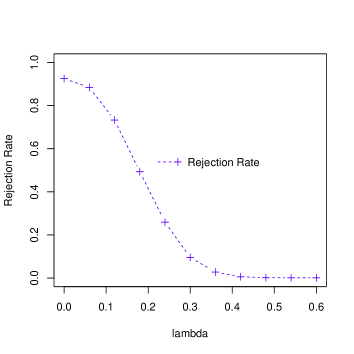
Figure 2: Simulated rejection probabilities of the test for lag-$1$ correlation as a function of the threshold $\delta\in[0,2\Delta]$ in the hypothesis (1.3) for Model III.

Importantly, the symmetry of the innovations do not affect the asymptotic properties of the tests, since the rates of Gaussian approximations of partial sums from skewed random variables are of the same order as in the symmetric case. To investigate if there exist differences in the finite sample properties we took model II and III, with the $i.i.d.$ Gaussian innovations replaced by $i.i.d$ $(\chi^{2}(5)-5)/\sqrt{10}$ random variables. In Table 3 we display the simulated type I error of the test (3.15) for a change point in the lag-$1$ correlation in model $II$ and of the test (4.15) for a relevant change point in the lag-$1$ correlation in model $III$. The corresponding results for a symmetric error can be found in Tables 1 and 2; we only observe minor differences in the approximation of the nominal level between the symmetric and non-symmetric case.

Table 3: Simulated type I error of the test (3.15) for a change point in the lag-$1$ correlation in model $II$ and of the test (4.15) for a relevant change point test in lag-$1$ correlation (at the boundary point of the null) in model $III$ with $(\chi^{2}(5)-5)/\sqrt{10}$ innovations. The last column represents the simulated Type I error if the bandwidth is $b_{n}$ selected by GCV.

II model	$b_{n}$	0.075	0.1	0.125	0.15	0.175	0.2	0.225	GCV
	5%	4.6	4.55	3.6	2.6	2.95	3.25	2.9	4.2
	10%	10.35	8.95	8.7	7.15	7.65	7.35	6.8	9.3
III	5%	4.85	5.1	4.95	6.9	5.25	6	5.35	5.4
	10%	8.9	8.85	9.7	11.7	9.9	10.35	9.85	9.95

Remark 5.1.

Throughout, the bandwidth $b_{n}$ is assumed to be the same over the whole sequence. As pointed out by one referee, it might be of interest to investigate a time-dependent bandwidth $b_{n}$ with respect to its potential to deal with local stationarity. Using similar arguments as in Zhou and Wu, (2009) we can obtain the optimal time varying bandwidth as

$$b_{n}(t)=\left|\frac{\hat{\kappa}(t)}{\hat{\sigma}(t)}\right|b_{n},$$ (5.1)

where $b_{n}$ is the time invariant bandwidth obtained by the GCV method, $\hat{\kappa}^{2}$ and $\hat{\sigma}^{2}$ are estimates of the long run variance and the variance of the random variables $e_{i}$, respectively. It is hard to accurately estimate $\kappa^{2}$ in a PLS model due to the unknown break points. In the case of local stationarity, an estimate of $\kappa^{2}$ was proposed by Zhou and Wu, (2010) and we used this method to investigate the differences between a local and global bandwidth in the locally stationary model I. The simulated levels of the corresponding bootstrap tests are shown in Table 4 and we observe that the performance of the procedure with a time dependent bandwidth is quite similar to the one using a constant bandwidth.

Table 4: Simulated type I error of the test (3.15) for a change point in the lag-$1$ correlation in model I using the time varying bandwidth (5.1). The last column represents the simulated Type I error if the bandwidth is $b_{n}$ selected by GCV.

Model I	$b_{n}$	0.075	0.1	0.125	0.15	0.175	0.2	0.225	GCV
	5%	5.05	4.9	4.3	3.95	4.2	3.15	3.55	4.15
	10%	10.45	9.75	9.5	9.85	8.9	7.55	8	10.7

5.2 Some robustness considerations

As was pointed out by a referee it might be of interest to investigate the approximation of the nominal level if the assumption of PLS is violated. For this purpose we considered modifications of the models $II$ and $III$ introduced in the previous section. Let $\{\eta_{i},i\in\mathbb{Z}\}$ denote $i.i.d.$ standard normal distributed and $\{\varepsilon_{i},i\in\mathbb{Z}\}$ denote $i.i.d$ $t$-distributed random variables with $5$ degrees of freedom, normalized such that they have variance $1$. We consider the processes

($II_{0}$) $G_{i}=H_{i}\sqrt{c(i/n)}/2$ for $i/n\leq 0.5$, and $G_{i}=H_{i}\sqrt{d(i/n)}/2$ for $i/n>0.5$, where $c(t)=1-(t-0.5)^{2}$, $d(t)=1-\frac{1}{2}\sin t$ and $H_{i}=0.2H_{i-1}+\varepsilon_{i}$ for $i/n\leq 0.5$, and $H_{i}=0.2H_{i-1}+\eta_{i}$ for $i/n>0.5$.

($III_{0}$) $G_{i}=H_{i}\sqrt{1-(i/n-0.5)^{2}}/2$, where $H_{i}=0.1H_{i-1}+\varepsilon_{i}$ for $i/n\leq 0.5$, and $H_{i}=0.4H_{i-1}+\eta_{i}$ for $i/n>0.5$.

These models are not PLS in the sense of Definition 2.1. In Table 5 we show the simulated type I error of the test (3.15) for a change point in the lag-$1$ correlation in model $II_{0}$ and of the test (4.15) for a relevant change point test in the lag-$1$ correlation in model $III_{0}$. We observe reasonable approximations of the nominal level in all cases under consideration.

Table 5: Simulated type I error of the test (3.15) for a change point in the lag-$1$ correlation in model $II_{0}$ and of the test (4.15) for a relevant change point test in the lag-$1$ correlation (at the boundary point of the null) in model $III_{0}$. The last column represents the simulated Type I error if the bandwidth is $b_{n}$ selected by GCV.

$II_{0}$	$b_{n}$	0.075	0.1	0.125	0.15	0.175	0.2	0.225	GCV
	5%	4.45	3.9	3.8	4.15	2.9	3	2.85	3.6
	10%	9.8	9.2	9.2	8.4	7	7.55	6.7	8.55
$III_{0}$	5%	6.25	5.75	5.9	5.2	6.2	6.05	4.7	4.6
	10%	10.15	10	10.1	9.7	11.4	10.8	8.8	8.35

In fact, it follows from Zhou, (2012) that model $II_{0}$ and $III_{0}$ can be approximated by the two PLS models

($II_{0}^{*}$). $G(t,\mathcal{F}_{i})=H(t,\mathcal{F}_{i})\sqrt{c(t)}/2$ for $t\leq 0.5$, and $G(t,\mathcal{F}_{i})=H(t,\mathcal{F}_{i})\sqrt{d(t)}/2$ for $t>0.5$, where $c(t)=1-(t-0.5)^{2}$, $d(t)=1-\frac{1}{2}\sin t$ and $H(t,\mathcal{F}_{i})=0.2H(t,\mathcal{F}_{i-1})+\varepsilon_{i}$ for $t\leq 0.5$, and $H(t,\mathcal{F}_{i})=0.2H(t,\mathcal{F}_{i-1})+\eta_{i}$ for $t>0.5$.

($III_{0}^{*}$). $G(t,\mathcal{F}_{i})=H(t,\mathcal{F}_{i})\sqrt{1-(t-0.5)^{2}}/2$, where $H(t,\mathcal{F}_{i})=0.1H(t,\mathcal{F}_{i-1})+\varepsilon_{i}$ for $t\leq 0.5$, and $H(t,\mathcal{F}_{i})=0.4H(t,\mathcal{F}_{i-1})+\eta_{i}$ for $t>0.5$,

where $\mathcal{F}_{i}=(\eta_{-\infty}\varepsilon_{-\infty}...,\eta_{0},\varepsilon_{0},...,\eta_{i},\varepsilon_{i})$. In summary, the proposed test procedures work reasonably well as long as the underlying processes are not too different from PLS processes. An important class of non-stationary processes that are not PLS and cannot be handled by our methodology are the unit root non-stationary processes.

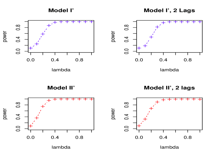
Figure 3: Simulated power. Upper left panel: test for a constant lag-$1$ correlation defined in (3.15) (model (I’)). Upper right panel: test for constant lags-$1$ and lag-$2$ correlation defined in (3.15) (model (I’)). Lower left panel: test for the hypothesis of a non-relevant change in the lag-$1$ correlation defined in (4.15) (model (II’)). Lower right panel: test for the hypothesis of a non-relevant change in the lag-$1$ and lag-$2$ correlation defined in (4.15) (model (II’)).

5.3 Power properties

In this section we investigate the power of the proposed tests in two scenarios. Let $\{\varepsilon_{i}\}_{i\in\mathbb{Z}}$ be $i.i.d$ N(0,1).

(I’) $G(t,\mathcal{F}_{i})=H(t,\mathcal{F}_{i})\sqrt{c(t)}/2$ for $t\leq 0.5$, and $G(t,\mathcal{F}_{i})=H_{1}(t,\mathcal{F}_{i})\sqrt{c(t)}/2$ for $t>0.5$, where $c(t)=1-(t-0.5)^{2}$, $H(t,\mathcal{F}_{i})=0.2H(t,\mathcal{F}_{i-1})+\varepsilon_{i}$ for $t\leq 0.5$, and $H(t,\mathcal{F}_{i})=(0.2-\lambda)H(t,\mathcal{F}_{i-1})+\varepsilon_{i}$ for $t>0.5$.

(II’) $G(t,\mathcal{F}_{i})=H(t,\mathcal{F}_{i})\sqrt{1-(t-0.5)^{2}}/2$, where $H(t,\mathcal{F}_{i})=(0.1-\lambda)H(t,\mathcal{F}_{i-1})+\varepsilon_{i}$ for $t\leq 0.5$, and $H(t,\mathcal{F}_{i})=0.4H(t,\mathcal{F}_{i-1})+\varepsilon_{i}$ for $t>0.5$.

Model (I’) is used to study the power of the test (3.15) for the “classical” hypothesis of no change point in the correlation for various values of $\lambda$, where $\lambda=0$ corresponds to the null hypothesis of a constant correlation. In the upper panel of Figure 3 we show the simulated power of the test for a constant lag-$1$ correlation while in the upper right panel corresponding results of the test for a constant lag-$1$ and lag-$2$ correlations are displayed. We observe a decrease in power, which can be explained by the observation, that in model (I’) the jump size of the lag $2$-correlation is $|0.2^{2}-(0.2-\lambda)^{2}|$, which is not monotone with respect to $\lambda$. The power properties of the test (4.15) of a change is investigated in model (II’). In the lower left panel of Figure 3 we display the simulated rejection probabilities for the hypotheses of a non-relevant change in the lag-$1$ correlation, that is

$$H_{0}:\Delta_{1}\leq 0.3~{}\mbox{ versus }~{}H_{1}:\Delta_{1}>0.3,$$

where $-0.6\leq\lambda\leq 0$ corresponds to the null hypothesis. In the lower right panel we investigate the hypotheses for lag-$1$ and lag-$2$ correlations, that is

$$H_{0}:\Delta_{1}\leq 0.3\ \text{and}\ \Delta_{2}\leq 0.15~{}\mbox{ versus }~{}H_{1}:\Delta_{1}>0.3\ \text{or}\ \Delta_{2}>0.15,$$

where $0.1-\sqrt{0.31}\leq\lambda\leq 0$ corresponds to the null hypothesis. We observe a decrease in power (note again that, the jump size of the lag $2$-correlation is $|0.4^{2}-(0.1-\lambda)^{2}|$, which is not monotone with respect to $\lambda$). We conclude that in all cases under consideration the proposed methodology can detect (relevant) changes in the correlation structures with reasonable size.

Remark 5.2.

The power of the proposed tests depends sensitively on the choice of the bandwidth $b_{n}$. Ideally, if the errors are $i.i.d$ or the series is strictly stationary, the optimal bandwidth can be calculated by an Edgeworth-expansion-based method (see Gao and Gijbels, (2008)) such that the power is optimized. However, the extension of this approach to a PLS scenario is non-trivial, and is out of the present scope but an interesting problem for future work. In the case of a stationary null hypothesis, we have also compared the power of our test presented with algorithms specifically designed for stationary processes. We observed that our approach has decent power; these results are presented in Section LABEL:StationaryPerformance of the supplementary material.

6 Data Analysis

Figure 4: Percentage change (left panel) and the squared percentage change (right panel) of exchange rate of USD/CAD. The line in the right panel is the fitted mean for the squared percentage change.

Figure 5: p-values of the bootstrap test for a relevant change in the lag-$1$, lag-$2$ and lag-($1$, $2$) correlations for the squared percentage change of USD/CAD for different values of the threshold $\delta$. The horizontal line marks the significance level $0.05$.

Table 6: Tests for the existence of a change point in the lag-$1$ and lag-$2$ correlations of the USD/CAD series, respectively. $v^{*}_{\alpha}$ denotes the critical values obtained by the bootstrap procedure. “Whole” represents the whole period, “Before” and “After” represent the period before and after the detected change date.

	lag $1$-Correlation			lag $2$-Correlation
	Whole	Before	After	Whole	Before	After
Test Stat.	1.28*	0.50	0.99	1.38**	0.40	2.74
$v^{*}_{90\%}$	1.23	0.70	1.01	1.15	0.72	3.95
$v^{*}_{95\%}$	1.36	0.78	1.12	1.3	0.80	4.70
$b_{n}$	0.34	0.18	0.54	0.34	0.29	0.15
$m$	18	9	22	18	18	12
$c_{n}$	0.13	0.24	0.19	0.13	0.14	0.34

We analyze the daily exchange rate of U.S. dollar/Canadian dollar from Nov 18th, 2011 to Jun 24th, 2016. The data can be obtained from https://www.federalreserve.gov/releases
/h10/hist/. The series contains 1154 data points. During the period, USD/CAD has changed drastically in the range (0.9710, 1.4592). The wide range of the exchange rate motivates us to further investigate the robustness of the volatility of the percentage change of the series during the period. Figure 4 shows the percentage change and squared percentage change of the exchange rate data. The pattern of the squared percentage change of exchange rate displays non-stationarity. For the test over the whole period, the GCV method selects $b_{n}=0.34$ and $c_{n}=0.3$ and the MV method select $m=18$. For this section, the critical values were generated by $8000$ bootstrap replications. We used the statistic (3.5) to estimate the abrupt change points in the variance with $\zeta=0.10$ and $L=31$, and identified a variance change point $t^{*}_{n}=795$, which corresponds to Jan 15th, 2015.

Let $X_{t}$ represent the squared percentage change at day $t$, and consider the relationship between $X_{t}$ and $X_{t-i}$, $i=1,2,3$. We performed our test on lag $1$, $2$ and $3$ simultaneously to check two null hypothesis: (i) all three correlations are $0$, (ii) all three correlations stay constant during the time considered. For (ii), we use the testing procedure in Section 3. For testing (i), we modified the test procedure in Section 3 by setting ${T}_{n}$ in (3.9) as ${T}_{n}=\max_{1\leq i\leq n}|{\mathbf{S}}_{i}|$. The test statistic is the corresponding quantity $\hat{T}_{n}$ that replaces the error in $T_{n}$ by the local linear residuals. The critical value was generated by the bootstrap sample of $\max_{m+1\leq i\leq n-m+1}|{\hat{\mathbf{\Phi}}}_{i,m}|$ where $\hat{\mathbf{\Phi}}_{i,m}$ is defined in (3.14). For null hypothesis (i), the test statistics was 4.05, with simulated $p$-Value 1.2%. For null hypothesis (ii), the test statistics was 2.09 with simulated $p$-value 4.5%. Hence there is moderately strong evidence that there are non-zero and non-constant correlations among the three lags.

We analyzed the correlation at lags 1,2,3 separately. We tested the constancy in the lag-$1$ correlation for squared percentage change. The $p$-value for the test of no change points in the lag-$1$ correlation was $7.6\%$. (see Table 6), and the $p$-value for null hypothesis (i) of zero lag-1 correlation was $4.1\%$. Next we used the statistic (4.4) to identify the location of the change point of the first order correlation and found $\hat{t}_{n}=397$, which corresponds to Jun 18th, 2013. We investigated the existence of further changes in the lag-$1$ correlation before and after the Jun 18th, 2013 and concluded that there are no further structural breaks in the lag-$1$ correlation during the two periods at $5\%$ significance level, with the $p$-value $40\%$ and $11\%$, respectively, for the first and second period. For the first period, the test statistic for zero lag-$1$ correlation was $1.98$ with $p$-value $<$ $1\%$. For the second period, the test statistic for zero lag-1 correlation was 2.25 with $p$-value $1.1\%$. The identified change point in the lag-$1$ correlation is close to the date that USD/CAD significantly exceeded the boundary $1$. Before this date, the exchange rate was slightly fluctuating around $1$, and after this point the exchange rate increased over 1.4 and never returned to $1$.

For lag-2, the testing result are also presented in Table 6. There $p$-value for the test of hypothesis of zero lag-2 correlation is $<1\%$, while the $p$-value of constant lag-2 correlation is $2.7\%$. The location of the jump time for the lag-2 correlation is 695 which corresponds to Aug 25, 2014. We also investigated the lag-2 correlation before and after Aug 25, 2014. For the hypothesis of constant lag-2 correlation, The $p$-values were $71\%$ and $26\%$ for the first and second period, respectively. For the hypothesis of zero lag-2 correlation, the $p$-values were $1\%$ and $18\%$ before and after the jump, respectively. The identified change point in the lag-$2$ correlation is close to the date where the Crude oil price drastically decreased from 100 USD per barrel to 50 USD per barrel. The oil price has a great impact on the economy of Canada, which is one of the decisive factors of the exchange rate.

For lag-3, the test statistic for no changes in correlation was 0.96 with $p$-value $43.3\%$. The test statistic for zero lag-3 correlation was 1.11 with $p$-value $58.9\%$. We conclude that correlations of the squared percentage changes concentrate in lag-1 and lag-2, with change points existing in both lags. Interestingly, the time of change for lag-1 and 2 correlations are different.

We further performed tests from Section 4 for relevant changes in lag-1, lag-2 correlations separately and jointly (the trajectory we considered was $\delta_{1}=\delta_{2}$) for the USD/CAD data. The estimates of the lag-$1$ correlation before and after the break point were $-0.056$ and $0.079$ while, for the lag-2 correlation, the estimates before and after the jump were $0.092$ and $-0.034$. The $p$-values of the tests for a relevant change in the lag-$1$/lag-$2$ correlation for different values of the threshold $\delta$ are displayed in Figure 5. At 5% significance level, we conclude that there are relevant changes with size $\delta=0.032$ in the lag-$1$ correlation, $\delta=0.024$ in the lag-2 correlation, and size $\delta=0.026$ in lag-1 or lag-2 correlation. The $p$-values of the tests for relevant changes in the lag-$1$ or $2$ correlation for different values of the threshold $\delta$ for the USD/CAD are displayed in Figure 5.

The correlations of the squared series are closely related to the ARCH effect. For example, Baillie and Chung, (2001) estimated the GARCH model via the autocorrelations of the square of the process. Our method shows that the USD/CAD from late 2011-mid 2016 may not be well fitted by a simple ARCH/GARCH model due to the changes in the correlation structure. Further, the negative first order correlation in the first period shows that USD/CAD from late 2011-mid 2013 may not be well fitted by usual ARCH/GARH model, due to their restriction of positive coefficients. Other models, for example the EGARCH model should be considered. We have also identified very different pattern of squared percentage changes of USD/CAD in the three lags considered: there is weak evidence against the null hypothesis of constant lag-1 correlation, strong evidence against constant lag-2 correlation, no evidence against constant lag-3 correlation, and strong evidence against constant lag-1, lag-2 and lag-3 correlations. We have no evidence against zero lag-3 correlation, while we have strong evidence against the hypotheses of zero lag-1 or lag-2 correlations.

7 Supplementary Materials

The supplementary materials contains the proofs of theorems and additional simulation results.  
 
Acknowledgements. The work of H. Dette has been supported in part by the Collaborative Research Center “Statistical modeling of nonlinear dynamic processes” (SFB 823, Teilprojekt A1, C1) of the German Research Foundation (DFG). Z. Zhou’s research has been supported in part by NSERC of Canada. The authors would like to thank Martina Stein who typed parts of this manuscript with considerable technical expertise. The authors would also like to thank three referees and an associate editor for their constructive comments on an earlier version of this paper.

See pages - of proof-Sep-02-2017

References

- Abraham and Wei, (1984) Abraham, B. and Wei, W. W. S. (1984). Inferences about the parameters of a time series model with changing variance. Metrika 31,183–194.
- Ahamada, Jouini and Boutahar, (2004) Ahamada, I. and Jouini, J. and Boutahar, M. (2004). Detecting multiple breaks in time series covariance structure, A nonparametric approach based on the evolutionary spectral density. Applied Economics 36,1095–1101.
- Andrews, (1993) Andrews, D. W. K. (1993). Tests for parameter instability and structural change with unknown change point. Econometrica 61(4),128–156.
- Aue et al., (2009) Aue, A., Hörmann, S., Horváth, L., and Reimherr, M. (2009). Break detection in the covariance structure of multivariate time series models. Annals of Statistics 37(6),4046–4087.
- Aue and Horváth, (2013) Aue, A. and Horváth, L. (2013). Structural breaks in time series. Journal of Time Series Analysis 34(1),1–16.
- Baufays and Rasson, (1985) Baufays, P. and Rasson, J. P. (1985). Variance changes in autoregressive models. In Anderson, D., editor, Time Series Analysis, Theory and Practice 7 pages 119–127. North-Holland, New York.
- Baillie and Chung, (2001) Baillie, Richard T., and Huimin Chung. (2001). Estimation of GARCH models from the autocorrelations of the squares of a process Journal of Time Series Analysis 22(6),631–650.
- Berger and Delampady, (1987) Berger, J. O. and Delampady, M. (1987). Testing precise hypotheses. Statistical Science 2(3),317–335.
- Berkes et al., (2009) Berkes, I. and Gombay, E. and Horvath, L. (2009). Testing for changes in the co-variance structure of linear processes. Journal of Statistical Planning and Inference 139,2044–2063.
- Berkson, (1938) Berkson, J. (1938). Some difficulties of interpretation encountered in the application of the chi-square test. Journal of the American Statistical Association 33(203),526–536.
- Bollerslev, (1986) Bollerslev, T. (1986). Generalized autoregressive conditional heteroskedasticity. Journal of econometrics 31(3), 307–327.
- Chen and Gupta, (1997) Chen, J. and Gupta, A. K. (1997). Testing and locating variance changepoints with application to stock prices. Journal of the American Statistical Association 92(438),739–747.
- Chow and Liu, (1992) Chow, S.-C. and Liu, P.-J. (1992). Design and Analysis of Bioavailability and Bioequivalence Studies. Marcel Dekker, New York.
- Dahlhaus, (1997) Dahlhaus, R., (1997). Fitting time series models to nonstationary processes. The Annals of Statistics 25(1), 1-37.
- Davis et al., (2006) Davis, R. A., Lee, T. C. M., and Rodriguez-Yam, G. A. (2006). Structural break estimation for nonstationary time series models. Journal of the American Statistical Association 101(473),223–239.
- Dette et al., (2011) Dette, H. and Preuß P. and Vetter, M. (2011). A measure of stationarity in locally stationary processes with applications to testing. Journal of the American Statistical Association 106,1113–1124.
- Dette and Wied, (2016) Dette, H. and Wied, D. (2016). Detecting relevant changes in time series models. Journal of the Royal Statistical Society, Ser., B 78,371–394.
- Dette et al., (2015) Dette, H., Wu, W. and Zhou, Z. (2015). Change point analysis of second order characteristics in non-stationary time series. arXiv,1503.08610 .
- Dwivedi and Subba Rao, (2011) Dwivedi, Y. and Subba Rao, S. (2011). A test for second order stationarity of a time series based on the discrete Fourier transform. Journal of Time Series Analysis 32,68–91.
- Engle, (1982) Engle, Robert F. (1982) Autoregressive conditional heteroscedasticity with estimates of the variance of United Kingdom inflation. Econometrica (1982), 987–1007.
- Fan and Gijbels, (1996) Fan, J. and Gijbels, I. (1996). Local Polynomial Modelling and its Applications. Chapman & Hall, London.
- Galeano and Peña, (2007) Galeano, P. and Peña, D. (2007). Covariance changes detection in multivariate time series. Journal of Statistical Planning and Inference 137,194–211.
- Gao and Gijbels, (2008) Gao, J. and Gijbels, I. (2008). Bandwidth Selection in Nonparametric Kernel Testing Journal of the American Statistical Association 103 1584–1594.
- Tong, (1990) Tong, H. (1990). Non-linear time series, a dynamical system approach Oxford , Oxford University Press.
- Inclán and Tiao, (1994) Inclán, C. and Tiao, G. C. (1994). Use of cumulative sums of squares for retrospective detection of changes of variance. Journal of the American Statistical Association 89(427).
- Jandhyala et al., (2013) Jandhyala, V., Fotopoulos, S., MacNeill, I., and Liu, P. (2013). Inference for single and multiple change-points in time series. Journal of Time Series Analysis 34(4),423–446.
- Jin et al., (2015) Jin, L. and Wang, S. and Wang, H. (2015). A new non-parametric stationarity test of time series in the time domain. Journal of the Royal Statistical Society, Series B 77,893–922.
- Killick et al., (2013) Killick, R. and Eckley, I. A. and Jonathan, P. (2013). A wavelet-based approach for detecting changes in second order structure within nonstationary time series. Electronic Journal of Statistics 7,1167–1183.
- Lee and Park, (2001) Lee, S. and Park, S. (2001). The cusum of squares test for scale changes in infinite order moving average processes. Scandinavian Journal of Statistics 28(4),625–44.
- Mallik et al., (2013) Mallik, A., Banerjee, M., and Sen, B. (2013). Asymptotics for -value based threshold estimation in regression settings. Electronic Journal of Statistics 7,2477–2515.
- Mallik et al., (2011) Mallik, A., Sen, B., Banerjee, M., and Michailidis, G. (2011). Threshold estimation based on a p-value framework in dose-response and regression settings. Biometrika 98,887–900.
- McBride, (1999) McBride, G. B. (1999). Equivalence tests can enhance environmental science and management. Australian New Zealand Journal of Statistics 41,19–29.
- Müller, (1992) Müller, H.-G. (1992). Change-points in nonparametric regression analysis. Annals of Statistics 20,737–761.
- Page, (1954) Page, E. S. (1954). Continuous inspection schemes. Biometrika 41,100–115.
- Paparoditis, (2009) Paparoditis, E. (2009). Testing temporal constancy of the spectral structure of a time series. Bernoulli 15,1190–1221.
- Paparoditis, (2010) Paparoditis, E. (2010). Validating stationarity assumptions in time series analysis by rolling local periodograms. Journal of the American Statistical Association 105,839–851.
- Paparoditis and Preuß, (2015) Paparoditis, E. and Preuß P. (2015). On local power properties of frequency domain-based tests for stationarity. Scandinavian Journal of Statistics 43,664-682.
- Politis et al., (1999) Politis, D. N., Romano, J. P., and Wolf, M. (1999). Subsampling. Springer, New York.
- Preuß et al., (2013) Preuß P. and Vetter, M. and Dette, H. (2013). A test for stationarity based on empirical processes. Bernoulli 19,2715–2749.
- Preuss et al., (2015) Preuss, P., Puchstein, R., and Dette, H. (2015). Detection of multiple structural breaks in multivariate time series. Journal of the American Statistical Association 110,654-668.
- Qu, (2008) Qu, Z. (2008). Testing for structural change in regression quantiles. Journal of Econometrics 148,170–184.
- Solomon, (2007) Solomon, S. (2007). Climate change 2007-the physical science basis, Working group I contribution to the fourth assessment report of the IPCC volume 4. Cambridge University Press.
- Vogt, (2012) Vogt, M. (2012). Nonparametric regression for locally stationary time series. The Annals of Statistics 40(5),2601–2633.
- Vogt and Dette, (2015) Vogt, M. and Dette, H. (2015). Detecting gradual changes in locally stationary processes. Annals of Statistics 43(2),713–740.
- Vostrikova, (1981) Vostrikova, L. J. (1981). Detecting ‘disorder’ in multidimensional random processes. Soviet Mathematics Doklady 24,55–59.
- Wichern et al., (1976) Wichern, D. W., Miller, R. B., and Hsu, D.-A. (1976). Changes of variance in first-order autoregressive time series models - with an application. Journal of the Royal Statistical Society. Ser. C (Applied Statistics) 25(3),248–256.
- Wied et al., (2012) Wied, D., Krämer, W., and Dehling, H. (2012). Testing for a change in correlation at an unknown point in time using an extended functional delta method. Econometric Theory 28(3),570–589.
- Wu, (2005) Wu, W. B. (2005). Nonlinear system theory, Another look at dependence. Proceedings of the National Academy of Sciences of the United States of America 102(40),14150–14154.
- Zhang and Wu, (2012) Zhang, T., and Wu, W. B. (2012). Inference of time-varying regression models. The Annals of Statistics 40(3), 1376–1402.
- Zhou and Wu, (2009) Zhou, Z. and Wu, W.B. (2009). Local linear quantile estimation for nonstationary time series. Annals of Statistics 2696-2729.
- Zhou and Wu, (2010) Zhou, Z. and Wu, W. B. (2010). Simultaneous inference of linear models with time-varying coefficients. Journal of the Royal Statistical Society, Series B 72,513–531.
- Zhou, (2012) Zhou, Z (2012). Measuring Nonlinear Dependence in Multivariate Time Series, A Distance Correlation Approach. Journal of Time Series Analysis 33, 438–457.
- Zhou, (2013) Zhou, Z. (2013). Heteroscedasticity and autocorrelation robust structural change detection. Journal of the American Statistical Association 108,726–740.
- Zhou, (2014) Zhou, Z. (2014). Inference of weighted -statistics for non-stationary time series and its applications. Annals of Statistics 42,87–114.