Mean-field theory of differential rotation in density stratified turbulent convection

Abstract

A mean-field theory of differential rotation in a density stratified turbulent convection has been developed. This theory is based on a combined effect of the turbulent heat flux and anisotropy of turbulent convection on the Reynolds stress. A coupled system of dynamical budget equations consisting in the equations for the Reynolds stress, the entropy fluctuations and the turbulent heat flux has been solved. To close the system of these equations, the spectral tau approach which is valid for large Reynolds and Peclet numbers, has been applied. The adopted model of the background turbulent convection takes into account an increase of the turbulence anisotropy and a decrease of the turbulent correlation time with the rotation rate. This theory yields the radial profile of the differential rotation which is in agreement with that for the solar differential rotation.

1 Introduction

Origin of the solar and stellar magnetic fields is associated with a mean-field dynamo (refereed as $\alpha\Omega$ or $\alpha^{2}\Omega$ dynamos) that is based on the combined effect of helical turbulent motions and a differential rotation (see, e.g., Moffatt, 1978; Parker, 1979; Krause & Rädler, 1980; Zeldovich et al., 1983; Rüdiger et al., 2013). A non-zero mean kinetic helicity produced by a rotating density stratified turbulent convection, causes the $\alpha$ effect in the solar convective zone. An origin of the solar differential rotation is related to an anisotropic eddy viscosity (Kippenhahn, 1963; Durney, 1985; Rüdiger, 1980, 1989). This idea has been applied in developing a theory of the differential rotation (Durney, 1993; Kichatinov & Rüdiger, 1993; Kitchatinov & Rüdiger, 2005). The turbulent heat flux in these theories has been introduced phenomenologically using the mixing-length theory relation: $\langle{\bf u^{\prime}}^{2}\rangle\propto g\tau_{0}\langle u^{\prime}_{z}s^{\prime}\rangle$, where $\langle u^{\prime}_{z}s^{\prime}\rangle$ is the vertical turbulent heat flux, ${\bf u}^{\prime}$ and $s^{\prime}$ are fluctuations of fluid velocity and entropy, ${\bf g}$ is the gravity acceleration and $\tau_{0}$ is the characteristic turbulent time. Also a quasi-linear approach that is valid for small fluid Reynolds numbers has been applied in these studies.

Additional possibility for the production of the solar differential rotation is associated with an effect of the turbulent heat flux on the Reynolds stress in a rotating density stratified turbulent convection. Based on this idea, Kleeorin & Rogachevskii (2006) develop a mean field theory of the differential rotation, where a coupled system of dynamical equations for the Reynolds stress, the entropy fluctuations and the turbulent heat flux has been solved adopting a spectral $\tau$ approach. It was demonstrated (Kleeorin & Rogachevskii, 2006) that the ratio of the contributions to the Reynolds stress caused by the turbulent heat flux and the anisotropic eddy viscosity is of the order of $\sim 10\,(H_{\rho}/\ell_{0})^{2}$, where $\ell_{0}$ is the maximum scale of turbulent motions and $H_{\rho}$ is the fluid density variation scale. This theory allows to determine the profiles of the differential rotation in the upper part of the solar convection zone where the rotation is slow in comparison with the turbulent time.

In the low part of the solar convective zone, the rotation is fast in comparison with the turbulent time. This causes a strong anisotropy of the turbulent convection that is an additional source of the solar differential rotation. One of the key theoretical questions is how can turbulent convection be modified by the fast rotation, and how can it affect the production of the differential rotation. This issue remains to be an open unresolved problem in the solar physics and astrophysics. Note that different theories of the solar differential rotation can be validated using data from the surface measurements of the solar angular velocity (see, e.g., Howard & Harvey, 1970; Snodgrass et al., 1984) and helioseismology based on measurements of the frequency of $p$-mode oscillations (see, e.g., Duvall et al., 1986; Dziembowski et al., 1989; Thompson, 1990; Kosovichev et al., 1997; Schou et al., 1998).

In the present study a combined effect of the turbulent heat flux and the turbulence anisotropy increasing with the rotation rate on the Reynolds stress has been studied for a rotating density stratified turbulent convection. The spectral tau approach which is valid for large Reynolds and Peclet numbers, has been used in this study. This allows us to advance the mean-field theory of the solar differential rotation and obtain the profiles of the differential rotation versus radius which are in agreement with the measured profiles of the solar differential rotation.

2 Effect of rotation on the Reynolds stress, entropy fluctuations and turbulent heat flux

To develop the theory of differential rotation in a small-scale density stratified turbulent convection, we use a mean-field approach whereby the velocity, pressure and entropy are decomposed into mean and fluctuating parts. This approach implies that there is a separation of temporal and spatial scales, so that the mean fields are varied in much larger scales in comparison with those for fluctuations.

Let us determine the dependencies of the Reynolds stresses $\langle u^{\prime}_{i}(t,{\bm{x}})\,u^{\prime}_{j}(t,{\bm{x}})\rangle$ and the turbulent heat flux $\langle s^{\prime}(t,{\bm{x}})\,u^{\prime}_{i}(t,{\bm{x}})\rangle$ on the mean fields, where angular brackets denote the ensemble averaging. To this end we use equations for fluctuations of velocity and entropy in a rotating turbulent convection, which are obtained by subtracting equations for the mean fields from the corresponding equations for the total fields. The equations for fluctuations of velocity ${\bm{u}}^{\prime}$ and entropy $s^{\prime}$ are given by

$${\partial{\bm{u}}^{\prime}\over\partial t} = -({\bm{U}}\cdot\mbox{\boldmath$\nabla$}){\bm{u}}^{\prime}-({\bm{u}}^{\prime}\cdot\mbox{\boldmath$\nabla$}){\bm{U}}-\mbox{\boldmath$\nabla$}\biggl{(}{p^{\prime}\over\rho_{0}}\biggr{)}-{\bm{g}}\,s^{\prime}+2{\bm{u}}^{\prime}\times{\bm{\Omega}}+{\bm{U}}^{N},$$ (1)

$${\partial s^{\prime}\over\partial t} = -{\Omega_{b}^{2}\over g}({\bm{u}}^{\prime}\cdot{\bm{e}})-({\bm{U}}\cdot\mbox{\boldmath$\nabla$})s^{\prime}+S^{N}.$$ (2)

Equations (1) and (2) are written in the reference frame rotating with the angular velocity ${\bm{\Omega}}$. Here $p^{\prime}$ are fluctuations of fluid pressure, the entropy fluctuations are determined by $s^{\prime}=(\gamma P_{0})^{-1}p^{\prime}-\rho_{0}^{-1}\rho^{\prime}$, the mean fields ${\bm{U}}$ and $S$ are the mean velocity and entropy, ${\bm{e}}$ is the unit vector directed opposite to ${\bm{g}}$ and $\Omega_{b}^{2}=-{\bm{g}}\cdot\mbox{\boldmath$\nabla$}S$. The fluid velocity for a low Mach number flows satisfies the continuity equation written in the anelastic approximation, ${\rm div}\,(\rho_{0}\,{\bm{U}})=0$ and ${\rm div}\,(\rho_{0}\,{\bm{u}}^{\prime})=0$. The variables with the subscript $"0"$ correspond to the hydrostatic nearly isentropic basic reference state, i.e., $\mbox{\boldmath$\nabla$}P_{0}=\rho_{0}{\bm{g}}$ and ${\bm{g}}\cdot[(\gamma P_{0})^{-1}\mbox{\boldmath$\nabla$}P_{0}-\rho_{0}^{-1}\mbox{\boldmath$\nabla$}\rho_{0}]\approx 0$, where $\gamma$ is the ratio of specific heats. The turbulent convection is regarded as a small deviation from a well-mixed adiabatic reference state. The nonlinear terms ${\bm{U}}^{N}$ and $S^{N}$ in Eqs. (1) and (2) which include the molecular dissipative terms, are given by

$$U^{N} = \langle({\bm{u}}^{\prime}\cdot\mbox{\boldmath$\nabla$}){\bm{u}}^{\prime}\rangle-({\bm{u}}^{\prime}\cdot\mbox{\boldmath$\nabla$}){\bm{u}}^{\prime}+{\bm{f}}_{\nu}({\bm{u}}^{\prime}),$$

$$S^{N} = \langle({\bm{u}}^{\prime}\cdot\mbox{\boldmath$\nabla$})s^{\prime}\rangle-({\bm{u}}^{\prime}\cdot\mbox{\boldmath$\nabla$})s^{\prime}-(1/T_{0})\,\mbox{\boldmath$\nabla$}\cdot{\bm{F}}_{\kappa}({\bm{u}}^{\prime},s^{\prime}),$$

where $\rho_{0}\,{\bm{f}}_{\nu}({\bm{U}})$ is the mean molecular viscous force, ${\bm{F}}_{\kappa}({\bm{U}},S)$ is the mean heat flux associated with the molecular thermal conductivity.

To study the rotating turbulent convection we perform the derivations which include the following steps: (i) adopting new variables for fluctuations of velocity ${\bm{v}}=\sqrt{\rho_{0}}\,{\bm{u}}^{\prime}$ and entropy $s=\sqrt{\rho_{0}}\,s^{\prime}$; (ii) derivation of the equations for the second moments of the velocity fluctuations $\langle v_{i}\,v_{j}\rangle$, the entropy fluctuations $\langle s^{2}\rangle$ and the turbulent heat flux $\langle v_{i}\,s\rangle$ in the ${\bm{k}}$ space, where we apply a multi-scale approach (Roberts & Soward, 1975), which separates the mean fields varied in large scales from fluctuations varied in small scales; (iii) application of the spectral $\tau$ approximation and solution of the derived second-moment equations in the ${\bm{k}}$ space; (iv) returning to the physical space to obtain formulae for the Reynolds stress and the turbulent heat flux as the functions of the rotation rate.

Using Eqs. (27)-(28) for the fluctuations of velocity and entropy in ${\bm{k}}$ space derived in Appendix A, we obtain equations for the following correlation functions: $f_{ij}({\bm{k}},{\bm{K}})=\langle v_{i}(t,{\bm{k}}_{1})v_{j}(t,{\bm{k}}_{2})\rangle$, $F_{i}({\bm{k}},{\bm{K}})=\langle s(t,{\bm{k}}_{1})v_{i}(t,{\bm{k}}_{2})\rangle$, and $\Theta({\bm{k}},{\bm{K}})=\langle s(t,{\bm{k}}_{1})s(t,{\bm{k}}_{2})\rangle$, where ${\bm{k}}_{1}={\bm{k}}+{\bm{K}}/2$ and ${\bm{k}}_{2}=-{\bm{k}}+{\bm{K}}/2$. Here the wave vectors ${\bm{K}}$ and ${\bm{k}}$ are related to the large and small scales, respectively. Hereafter we omit the argument $t$ in the correlation functions to simplify notations. The equations for these second moments are given by

$${\partial f_{ij}({\bm{k}},{\bm{K}})\over\partial t} = \left(I_{ijmn}^{U}+L_{ijmn}^{\Omega}\right)\,f_{mn}+M_{ij}^{F}+\hat{\cal N}\tilde{f}_{ij},$$ (3)

$${\partial F_{i}({\bm{k}},{\bm{K}})\over\partial t} = \left(J_{im}^{U}+D_{im}^{\Omega}\right)\,F_{m}+ge_{m}P_{im}({\bm{k}}_{1})\,\Theta+\hat{\cal N}\tilde{F}_{i},$$ (4)

$${\partial\Theta({\bm{k}},{\bm{K}})\over\partial t} = -{\rm div}\,\left({\bm{U}}\Theta\right)+\hat{\cal N}\Theta,$$ (5)

where

$$I_{ijmn}^{U} = J^{U}_{im}({\bm{k}}_{1})\,\delta_{jn}+J^{U}_{jn}({\bm{k}}_{2})\,\delta_{im}=\biggl{[}2k_{iq}\delta_{mp}\delta_{jn}+2k_{jq}\delta_{im}\delta_{pn}-\delta_{im}\delta_{jq}\delta_{np}$$

$$\;-\delta_{iq}\delta_{jn}\delta_{mp}+\delta_{im}\delta_{jn}k_{q}{\partial\over\partial k_{p}}\biggr{]}\nabla_{p}U_{q}-\delta_{im}\delta_{jn}\,\left({\rm div}\,{\bm{U}}+{\bm{U}}{\bm{\cdot}}\mbox{\boldmath$\nabla$}\right),$$

$$M_{ij}^{F} = ge_{m}[P_{im}({\bm{k}}_{1})F_{j}({\bm{k}},{\bm{K}})+P_{jm}({\bm{k}}_{2})F_{i}(-{\bm{k}},{\bm{K}})],$$

and $L_{ijmn}^{\Omega}=D_{im}^{\Omega}({\bm{k}}_{1})\,\delta_{jn}+D_{jn}^{\Omega}({\bm{k}}_{2})\,\delta_{im}$, $\,J_{ij}^{U}({\bm{k}})=2k_{in}\nabla_{j}U_{n}-\nabla_{j}U_{i}-(1/2)\,{\rm div}\,{\bm{U}}\,\delta_{ij}$ and $D_{ij}^{\Omega}({\bm{k}})=2\varepsilon_{ijm}\Omega_{n}k_{mn}$. Here $\delta_{ij}$ is the Kronecker tensor, $k_{ij}=k_{i}k_{j}/k^{2}$, $\varepsilon_{ijk}$ is the Levi-Civita tensor, and $F_{i}(-{\bm{k}},{\bm{K}})=\langle s({\bm{k}}_{2})v_{i}({\bm{k}}_{1})\rangle$. The correlation functions $f_{ij}$, $\,F_{i}$ and $\Theta$ are proportional to the non-uniform fluid density $\rho_{0}$. Here $\hat{\cal N}\tilde{f}_{ij}$, $\,\hat{\cal N}\tilde{F}_{i}$ and $\hat{\cal N}\Theta$ are the terms which are related to the third-order moments appearing due to the nonlinear terms. In particular,

$$\hat{\cal N}\tilde{f}_{ij} = \langle P_{im}({\bm{k}}_{1})v^{N}_{m}({\bm{k}}_{1})v_{j}({\bm{k}}_{2})\rangle+\langle v_{i}({\bm{k}}_{1})P_{jm}({\bm{k}}_{2})v^{N}_{m}({\bm{k}}_{2})\rangle,$$

$$\hat{\cal N}\tilde{F}_{i} = \langle s^{N}({\bm{k}}_{1})u_{j}({\bm{k}}_{2})\rangle+\langle s({\bm{k}}_{1})P_{im}({\bm{k}}_{2})v^{N}_{m}({\bm{k}}_{2})\rangle,$$

$$\hat{\cal N}\Theta = \langle s^{N}({\bm{k}}_{1})s({\bm{k}}_{2})\rangle+\langle s({\bm{k}}_{1})s^{N}({\bm{k}}_{2})\rangle.$$

The equations for the second-order moments contain high-order moments and a closure problem arises (see, e.g., Monin & Yaglom, 2013; McComb, 1990). We apply the spectral $\tau$ approximation that is a sort of third-order closure procedure (see, e.g., Orszag, 1970; Pouquet et al., 1976; Kleeorin et al., 1990; Rogachevskii & Kleeorin, 2004). The spectral $\tau$ approximation postulates that the deviations of the third-order-moment terms, $\hat{\cal N}f_{ij}({\bm{k}})$, from the contributions to these terms afforded by the background turbulent convection, $\hat{\cal N}f_{ij}^{(0)}({\bm{k}})$, are expressed through the similar deviations of the second moments, $f_{ij}({\bm{k}})-f_{ij}^{(0)}({\bm{k}})$, i.e.,

$$\hat{\cal N}f_{ij}({\bm{k}})-\hat{\cal N}f_{ij}^{(0)}({\bm{k}})=-{f_{ij}({\bm{k}})-f_{ij}^{(0)}({\bm{k}})\over\tau_{r}(k)},$$ (6)

and similarly for other tensors, where $\hat{\cal N}f_{ij}=\hat{\cal N}\tilde{f}_{ij}+M_{ij}^{F}(F^{\Omega=0})$ and $\hat{\cal N}F_{i}=\hat{\cal N}\tilde{F}_{i}+ge_{n}P_{in}(k)\Theta^{\Omega=0}$, the superscript $(0)$ corresponds to the background turbulent convection (i.e., a turbulent convection with $\nabla_{i}U_{j}=0)$, $\,\tau_{r}(k)$ is the characteristic relaxation time of the statistical moments, which can be identified with the correlation time $\tau(k)$ of the turbulent velocity field for large Reynolds numbers. The quantities $F^{\Omega=0}$ and $\Theta^{\Omega=0}$ are for a nonrotating turbulent convection with nonzero spatial derivatives of the mean velocity. Validation of the $\tau$ approximation has been done in various numerical simulations and analytical studies (see, e.g., Brandenburg & Subramanian, 2005; Brandenburg et al., 2004, 2012a; Rogachevskii & Kleeorin, 2007; Rogachevskii et al., 2011, 2012; Käpylä et al., 2012). Note that we apply the $\tau$-approximation (6) only to study the deviations from the background turbulent convection which are caused by the spatial derivatives of the mean velocity. The background turbulent convection is assumed to be known (see below).

We use the following model of the background turbulent convection which takes into account an increase of the anisotropy of turbulence with increase of the rate of rotation:

$$f_{ij}^{(0)}\equiv\langle v_{i}({\bm{k}}_{1})\,v_{j}({\bm{k}}_{2})\rangle^{(0)} = {E(k)\,[1+2k\,\varepsilon_{u}\,\delta(k_{z})]\over 8\pi\,k^{2}\,(k^{2}+\tilde{\lambda}^{2})\,(1+\varepsilon_{u})}\Big{[}\delta_{ij}\,(k^{2}+\tilde{\lambda}^{2})-k_{i}\,k_{j}-\tilde{\lambda}_{i}\,\tilde{\lambda}_{j}$$ (7)

$$+i\,\big{(}\tilde{\lambda}_{i}\,k_{j}-\tilde{\lambda}_{j}\,k_{i}\big{)}\Big{]}\rho_{0}\,\langle{\bm{u}}^{\prime 2}\rangle^{(0)},$$

$$F_{i}^{(0)}\equiv\langle v_{i}({\bm{k}}_{1})\,s({\bm{k}}_{2})\rangle^{(0)} = {3\,E(k)\over 8\pi\,k^{4}}\Big{[}k^{2}\,e_{j}\,P_{ij}({\bm{k}})-i\tilde{\lambda}\,k_{j}\,P_{ij}({\bm{e}})\Big{]}\rho_{0}\,\langle s^{\prime}\,u^{\prime}_{z}\rangle^{(0)},$$ (8)

and $\Theta^{(0)}\equiv\langle s({\bm{k}}_{1})\,s({\bm{k}}_{2})\rangle^{(0)}=\rho_{0}\,\langle(s^{\prime})^{2}\rangle^{(0)}\,E(k)/4\pi k^{2}$, where $\mbox{\boldmath$\tilde{\lambda}$}=(\mbox{\boldmath$\lambda$}-\mbox{\boldmath$\nabla$})/2$, $\,\mbox{\boldmath$\lambda$}=-(\mbox{\boldmath$\nabla$}\rho_{0})/\rho_{0}$. We assume that the background turbulent convection is the Kolmogorov type turbulence with a constant flux of energy over the spectrum, i.e., the kinetic energy spectrum $E(k)=-d\bar{\tau}(k)/dk$, $\,\bar{\tau}(k)=(k/k_{0})^{1-q}$ with the exponent of the kinetic energy spectrum $1<q<3$, e.g., $q=5/3$ is for Kolmogorov spectrum. The turbulent correlation time $\tau(k)=2\tau_{{}_{\Omega}}\bar{\tau}(k)$, where $\tau_{{}_{\Omega}}=\ell_{0}/u_{0}$, and $\ell_{0}$ is the energy containing scale of turbulent motions, $u_{0}=\sqrt{\langle{\bm{u}}^{\prime 2}\rangle^{(0)}}$ is the characteristic turbulent velocity in the scale $\ell_{0}$ and $k_{0}=1/\ell_{0}$. We consider an anisotropic turbulent convection as a combination of a three-dimensional isotropic turbulence and two-dimensional turbulence in the plane perpendicular to the rotational axis. The degree of anisotropy $\varepsilon_{u}$ is defined as the ratio of turbulent kinetic energies of two-dimensional to three-dimensional motions. In this model we neglect effects which are O$(\lambda^{3},\nabla^{3}\langle{\bm{v}}^{2}\rangle^{(0)})$.

The effect of rotation on the turbulent correlation time is described just by an heuristic argument, i.e., we assume that $\tau_{\Omega}^{-2}=\tau_{0}^{-2}+\Omega^{2}/C_{\Omega}^{2}$, that yields:

$$\tau_{{}_{\Omega}}={\tau_{0}\over\left[1+\left(C_{{}_{\Omega}}^{-1}\,\Omega\,\tau_{0}\right)^{2}\right]^{1/2}}.$$ (9)

This implies that for fast rotation, $\Omega\,\tau_{0}\gg 1$, the parameter $\omega=8\Omega\,\tau_{{}_{\Omega}}$ tends to be limiting value $\omega_{m}=8C_{{}_{\Omega}}$, where the dimensionless constant $C_{{}_{\Omega}}\sim 1$.

The solution of Eqs. (3)–(5) after application of the spectral $\tau$ approximation, and the integration over the ${\bm{k}}$ space (see Appendix B) allow us to determine the Reynolds stress and the effective force versus angular velocity. The latter yields the mean-field equation for the differential rotation (see next section), which takes into account the effects of rotating density stratified turbulent convection.

3 Mean-field equation for differential rotation

The differential rotation in the axisymmetric fluid flow is determined by linearized Navier-Stokes equation for the toroidal component $U_{\varphi}(r,\theta)\equiv r\,\sin\theta\,\delta\Omega$ of the mean velocity:

$$\rho_{0}\,{\partial U_{\varphi}\over\partial t} = {1\over r^{3}}{\partial\over\partial r}(r^{3}\sigma_{r\varphi})+{1\over r\sin^{2}\theta}{\partial\over\partial\theta}(\sin^{2}\theta\,\sigma_{\theta\varphi})+2\,\rho_{0}\,({\bm{U}}{\bm{\times}}{\bm{\Omega}})_{\varphi},$$ (10)

where the tensor $\sigma_{ij}=-\langle v_{i}\,v_{j}\rangle$ is determined by the Reynolds stress:

$$\sigma_{r\varphi} \equiv -e_{j}^{\varphi}\,e_{i}^{r}\,\langle v_{i}\,v_{j}\rangle=\sigma_{r\varphi}^{\nu_{T}}+\sigma_{r\varphi}^{F}+\sigma_{r\varphi}^{u},$$ (11)

$$\sigma_{\theta\varphi} \equiv -e_{j}^{\varphi}\,e_{i}^{\theta}\,\langle v_{i}\,v_{j}\rangle=\sigma_{\theta\varphi}^{\nu_{T}}+\sigma_{\theta\varphi}^{F}+\sigma_{\theta\varphi}^{u}.$$ (12)

and ${\bm{e}}^{r}$, $\,{\bm{e}}^{\theta}$ and $\,{\bm{e}}^{\varphi}$ are the unit vectors along the radial, meridional and toroidal directions of the spherical coordinates $r,\theta,\varphi$. There are three contributions to the tensor $\sigma_{ij}=-\langle v_{i}\,v_{j}\rangle$ in Eqs. (11) and  (12). The first term in the right hand side of Eqs. (11) and  (12) describes the contribution $\sigma_{ij}^{\nu_{T}}$ to the Reynolds stress caused by turbulent viscosity $\nu_{{}_{T}}$:

$$\sigma_{r\varphi}^{\nu_{T}}=\rho_{0}\,\nu_{{}_{T}}\,r\,{\partial\over\partial r}\biggl{(}{U_{\varphi}\over r}\biggr{)},$$ (13)

$$\sigma_{\theta\varphi}^{\nu_{T}}=\rho_{0}\,\nu_{{}_{T}}\,{\sin\theta\over r}\,{\partial\over\partial\theta}\biggl{(}{U_{\varphi}\over\sin\theta}\biggr{)}.$$ (14)

The second term in Eqs. (11) and  (12) determines the contribution $\mbox{\boldmath$\sigma$}^{F}$ to the Reynolds stress caused by the turbulent heat flux:

$$\sigma_{r\varphi}^{F} = {1\over 6}\,\rho_{0}\,\tau_{{}_{\Omega}}^{2}\,g\,\langle s^{\prime}\,u^{\prime}_{z}\rangle^{(0)}\,\Omega\,\sin\theta\,[\Phi_{1}(\omega)+\cos^{2}\theta\,\Phi_{2}(\omega)]\;,$$ (15)

$$\sigma_{\theta\varphi}^{F} = {1\over 3}\,\rho_{0}\,\tau_{{}_{\Omega}}^{2}\,g\,\langle s^{\prime}\,u^{\prime}_{z}\rangle^{(0)}\,\Omega\,\sin^{2}\theta\,\cos\theta\,\Phi_{2}(\omega),$$ (16)

where the parameter $\omega=8\,\Omega\,\tau_{{}_{\Omega}}$. The functions $\Phi_{1}(\omega)$ and $\Phi_{2}(\omega)$ are given by Eqs. (36)–(38) in Appendix B and are shown in Fig. 1. When the turbulent correlation time is independent of the rotation rate, Eqs. (15) and (16) coincide with those obtained by Kleeorin & Rogachevskii (2006).

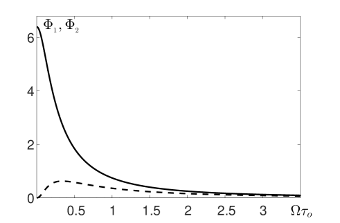
Figure 1: The functions $\Phi_{1}(\Omega\tau_{0})$ (solid) and $\Phi_{2}(\Omega\tau_{0})$ (dashed) versus $\Omega\tau_{0}$.

The third term in Eqs. (11) and (12) determines the contribution $\mbox{\boldmath$\sigma$}^{u}$ to the Reynolds stress caused by the anisotropy of turbulence due to the nonuniform fluid density and fast uniform rotation (see Eq. (35) in Appendix B):

$$\sigma_{r\varphi}^{u} = -{\lambda^{2}\,\ell_{0}^{2}\over 20}\,\rho_{0}\,\langle{\bm{u}}^{\prime 2}\rangle^{(0)}\,\tau_{{}_{\Omega}}\,\Omega\,\sin\theta\,(1+\cos^{2}\theta),$$ (17)

$$\sigma_{\theta\varphi}^{u} = {\lambda^{2}\,\ell_{0}^{2}\over 20}\,\rho_{0}\,\langle{\bm{u}}^{\prime 2}\rangle^{(0)}\,\tau_{{}_{\Omega}}\,\Omega\,\sin^{2}\theta\,\cos\theta.$$ (18)

Equation (10) in a steady-state that determines the profiles of the differential rotation, reads:

$$\hat{\cal W}(r)\,\rho_{0}\nu_{{}_{T}}\biggl{\{}{\partial\over\partial r}{\delta\Omega\over\Omega} + {1\over r}\,\Big{[}a_{F}\,\left(\Phi_{1}(\omega)+\Phi_{2}(\omega)X^{2}\right)-2a_{u}\,\lambda^{2}\ell_{0}^{2}\left(1+X^{2}\right)\Big{]}\biggr{\}}$$ (19)

$$- {\rho_{0}\nu_{{}_{T}}\over r^{2}}\,\hat{\cal M}(X)\,\biggl{\{}{\delta\Omega\over\Omega}-\Big{[}a_{F}\,\Phi_{2}(\omega)+a_{u}\lambda^{2}\ell_{0}^{2}\Big{]}\,X^{2}\biggr{\}}=0,$$

where the operators $\hat{\cal W}(r)$ and $\hat{\cal M}(X)$ are defined as

$$\hat{\cal W}(r)f(r)={1\over r^{4}}\,{\partial\over\partial r}\,\left[r^{4}f(r)\right],\quad\quad\hat{\cal M}(X)\phi(X)=\left[(X^{2}-1){\partial^{2}\over\partial X^{2}}+4X{\partial\over\partial X}\right]\phi(X),$$

$X=\cos\theta$, and the parameters $a_{F}$ and $a_{u}$ are given by $a_{F}=\tau_{\Omega}^{2}\,g\,\langle s^{\prime}\,u^{\prime}_{z}\rangle^{(0)}/6\,\nu_{{}_{T}}$ and $a_{u}=\tau_{\Omega}\,\langle{\bm{u}}^{\prime 2}\rangle^{(0)}/40\,\nu_{{}_{T}}$. We seek a solution of Eq. (19) in the form:

$${\delta\Omega\over\Omega}=\sum_{n=0}^{\infty}\,C_{2n}^{3/2}(X)\,\tilde{\Omega}_{2n}(r),$$ (20)

where the radius $r$ is measured in units of the solar radius $R_{\odot}$, and the function $C_{n}^{3/2}(X)$ satisfies the equation for the ultra-spherical polynomials:

$$[\hat{\cal M}(X)-n(n+3)]\,C_{n}^{3/2}(X)=0.$$ (21)

The function $C_{n}^{3/2}(X)$ has the following properties:

$$\int_{-1}^{1}\,(1-X^{2})\,C_{n}^{3/2}(X)\,C_{m}^{3/2}(X)\,dX={(n+1)(n+2)\over n+3/2}\,\delta_{nm},$$ (22)

$C_{0}^{3/2}(X)=1$ and $C_{2}^{3/2}(X)=(3/2)(5X^{2}-1)$. Substituting Eq. (20) into Eq. (19), we obtain equations for the functions $\tilde{\Omega}_{0}(r)$:

$$\tilde{\Omega}_{0}(r)=\tilde{\Omega}_{\ast}-{1\over 5}\int^{1}_{r/R_{\odot}}\Big{\{}12a_{u}\lambda^{2}\ell_{0}^{2}-a_{F}\,\left[5\Phi_{1}(\omega)+\Phi_{2}(\omega)\right]\Big{\}}\,{dr\over r},$$ (23)

and $\tilde{\Omega}_{2}(r)$:

$$\hat{\cal W}(r)\,\rho_{0}\nu_{{}_{T}}\,\biggl{[}{\partial\tilde{\Omega}_{2}(r)\over\partial r}+{2\over 15\,r}\,\Big{(}a_{F}\,\Phi_{2}(\omega)-2a_{u}\lambda^{2}\ell_{0}^{2}\Big{)}\biggr{]}$$

$$\quad\quad\quad\quad-{10\,\rho_{0}\nu_{{}_{T}}\over r^{2}}\biggl{[}\tilde{\Omega}_{2}(r)-{2\over 15}\left(a_{F}\,\Phi_{2}(\omega)+a_{u}\lambda^{2}\ell_{0}^{2}\right)\biggr{]}=0,$$ (24)

where $\tilde{\Omega}_{\ast}$ is the free constant determined by the surface boundary condition.

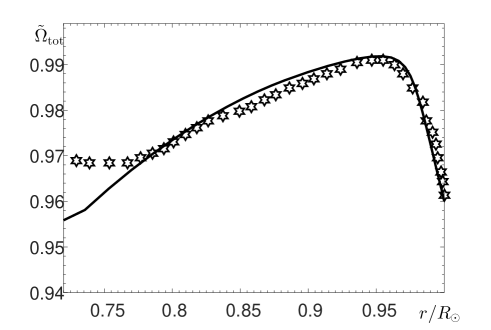
Figure 2: The total angular velocity $\tilde{\Omega}_{\rm tot}=\tilde{\Omega}_{0}+1$ that includes the uniform rotation $\Omega$ versus the radius $r/R_{\odot}$ (solid). This theoretical profile is compared with the radial profile of the solar angular velocity obtained from the helioseismology observational data (stars) at the latitude $\phi=30^{\circ}$ and normalized by the solar rotation frequency $\Omega_{\odot}(\phi=0)$ at the equator, where $R_{\odot}$ is the solar radius.

In Fig. 2 we show the total angular velocity $\tilde{\Omega}_{\rm tot}=\tilde{\Omega}_{0}+1$ that includes the uniform rotation $\Omega$ versus the radius $r/R_{\odot}$. This theoretical profile is compared with the radial profile of the solar angular velocity obtained from the helioseismology observational data (Kosovichev et al., 1997) specified for the latitude $\phi=30^{\circ}$ and normalized by the solar angular velocity $\Omega_{\odot}(\phi=0)$ at the equator. Note that at $\phi=30^{\circ}$ the contribution from the term $C_{2}^{3/2}(X)\,\tilde{\Omega}_{2}(r)$ to the differential rotation vanishes, because the function $C_{2}^{3/2}(X)=(3/2)(5X^{2}-1)$ at the angle around $\phi=30^{\circ}$ vanishes. To determine $\tilde{\Omega}_{\rm tot}$ we use the rotation rate dependence of the turbulent viscosity $\nu_{{}_{T}}(\omega)=\nu_{{}_{T}}^{\ast}\Phi_{\nu}(\omega)$, where $\nu_{{}_{T}}^{\ast}=\tau_{0}\langle{\bm{u}}^{\prime 2}\rangle^{(0)}/6$, the functions $\Phi_{\nu}(\omega)$ is given by Eq. (39) in Appendix B and is shown in Fig. 3. Strong change of the turbulent viscosity is caused by the fast rotation during the transition from isotropic three-dimensional turbulence to strongly anisotropic quasi two-dimensional turbulence.

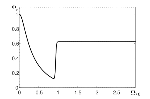
Figure 3: The rotation rate dependence of the functions $\Phi_{\nu}(\Omega\tau_{0})$, where $\nu_{{}_{T}}(\Omega\tau_{0})=\nu_{{}_{T}}^{\ast}\Phi_{\nu}(\Omega\tau_{0})$.

For the comparison of the theoretical profiles of the differential rotation and observational data, we use the radial profiles of $\Omega\,\tau_{0}(r)$ (see Fig. 4) and the ratio $\ell_{M}(r)/H_{\rho}(r)$ (see Fig. 5) of the mixing length $\ell_{M}$ to the density stratification length $H_{\rho}$ based on the model of the solar convective zone by Spruit (1974). Inspection of Fig. 2 demonstrates that the theoretical profile of the differential rotation is in agreement with the profile of the solar differential rotation when $\ell_{M}/\ell_{0}=5$. The latter is justified by the results of analytical study (Elperin et al., 2002, 2006) and laboratory experiments (Bukai et al., 2009), which show that the integral scale $\ell_{0}$ of the turbulent convection is smaller in 5 times in comparison with the size of the coherent structures (the large-scale circulations). We compare the theoretical and observation profiles of the differential rotation for the latitude $\phi=30^{\circ}$ because for the latitudes which are far from $\phi=30^{\circ}$, the contribution of the term $\propto\tilde{\Omega}_{2}$ (determined by Eq. (24)) to the differential rotation cannot be ignored. More detail comparison of the theoretical and observation profiles of the differential rotation for different latitudes requires the mean-field numerical modelling that is a subject of the separate study.

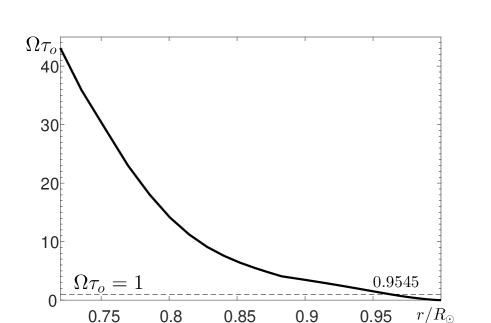
Figure 4: The profile of $\Omega\tau_{0}$ versus $r/R_{\odot}$ based on the model of the solar convective zone by Spruit (1974).

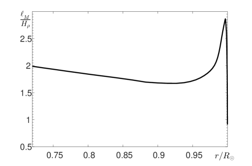
Figure 5: The profile of the ratio $\ell_{M}/H_{\rho}$ of the mixing length $\ell_{M}$ to the density stratification length $H_{\rho}$ versus $r/R_{\odot}$ that is based on the model of the solar convective zone by Spruit (1974).

4 Conclusions

We discuss a new theory of differential rotation based on a combined effect of the turbulent heat flux and the turbulence anisotropy increasing with the rate of rotation on the Reynolds stress in a density stratified turbulent convection. We solve a coupled system of dynamical budget equations which includes the equations for the Reynolds stress, the entropy fluctuations and the turbulent heat flux, applying a spectral $\tau$ approach to close the system of these equations. The model of the background turbulent convection takes into account an increase of the turbulence anisotropy and a decrease of the turbulent correlation time with the rotation rate. This theory allows to obtain the profile of the differential rotation versus radius which is in agreement with the profile of the solar differential rotation.

The mechanism of the differential rotation that is related to the effect of the turbulent heat flux on Reynolds stress in a rotating turbulent convection is as follows. The total angular velocity includes the uniform rotation $\Omega$ and the differential rotation $\delta\Omega$. The uniform rotation results in the counter-rotation turbulent heat flux $\langle s^{\prime}\,u^{\prime}_{\varphi}\rangle$ that is directed opposite to the uniform rotation $\Omega$. The counter-rotation turbulent heat flux is similar to the counter-wind turbulent heat flux that is directed opposite to the mean wind known in the atmospheric physics (Elperin et al., 2002, 2006). In turbulent convection an ascending fluid element obeys larger temperature than the temperature of the surrounding fluid and smaller toroidal fluid velocity, while a descending fluid element obeys smaller temperature and larger toroidal fluid velocity. This results in the turbulent heat flux in the direction opposite to the uniform rotation. The entropy fluctuations produce fluctuations of the buoyancy force, that increases fluctuations of the vertical and meridional components of the velocity which are correlated with the fluctuations of the toroidal component of the velocity. This implies that the off-diagonal components of the Reynolds stress, $\langle u^{\prime}_{r}u^{\prime}_{\varphi}\rangle$ and $\langle u^{\prime}_{\theta}u^{\prime}_{\varphi}\rangle$ are non-zero, producing the toroidal component of the effective force. The latter results in the formation of the differential rotation $\delta\Omega$ in turbulent convection.

Appendix A Derivation of equations for the second moments

Equations (1) and (2) in the new variables for fluctuations of velocity ${\bm{v}}=\sqrt{\rho_{0}}\,{\bm{u}}^{\prime}$ and entropy $s=\sqrt{\rho_{0}}\,s^{\prime}$ are given by

$${1\over\sqrt{\rho_{0}}}{\partial{\bm{v}}({\bm{x}},t)\over\partial t} = -\mbox{\boldmath$\nabla$}\biggl{(}{p^{\prime}\over\rho_{0}}\biggr{)}+{1\over\sqrt{\rho_{0}}}\biggl{[}2{\bm{v}}{\bm{\times}}{\bm{\Omega}}-({\bm{v}}\cdot\mbox{\boldmath$\nabla$}){\bm{U}}-G^{U}\,{\bm{v}}-{\bm{g}}\,s\biggr{]}+{\bm{F}}_{M}+{\bm{v}}^{N},$$

$${\partial s({\bm{x}},t)\over\partial t} = -{\Omega_{b}^{2}\over g}({\bm{v}}\cdot{\bm{e}})-G^{U}\,s+s^{N},$$ (26)

where $G^{U}=(1/2)\,{\rm div}\,{\bm{U}}+{\bm{U}}{\bm{\cdot}}\mbox{\boldmath$\nabla$}$, $\,{\bm{v}}^{N}$ and $s^{N}$ are the nonlinear terms which include the molecular viscous and dissipative terms. The fluid velocity fluctuations ${\bm{v}}$ satisfy the equation $\mbox{\boldmath$\nabla$}\cdot{\bm{v}}={\bm{v}}\cdot{\bm{\lambda}}/2$.

Let us derive equations for the second-order moments. For this purpose we rewrite the momentum equation and the entropy equation in a Fourier space. In particular,

$${dv_{i}({\bm{k}})\over dt} = [D_{im}^{\Omega}({\bm{k}})+\tilde{J}_{im}^{U}({\bm{k}})]v_{m}({\bm{k}})+g\,e_{m}\,P_{im}({\bm{k}})\,s({\bm{k}})+v_{i}^{N}({\bm{k}}),$$ (27)

$${ds({\bm{k}})\over dt} = -G^{U}({\bm{k}})\,s({\bm{k}})+s^{N},$$ (28)

where

$$\tilde{J}_{ij}^{U}({\bm{k}})=2k_{in}\nabla_{j}U_{n}-\nabla_{j}U_{i}-G^{U}({\bm{k}})\delta_{ij},\quad G^{U}({\bm{k}})={1\over 2}\,{\rm div}\,{\bm{U}}+i({\bm{U}}{\bm{\cdot}}{\bm{k}}),$$

$D_{ij}^{\Omega}({\bm{k}})=2\varepsilon_{ijm}\Omega_{n}k_{mn}$, $\delta_{ij}$ is the Kronecker tensor, $k_{ij}=k_{i}k_{j}/k^{2}$ and $\varepsilon_{ijk}$ is the Levi-Civita tensor. To derive Eq. (27) we multiply the momentum equation written in ${\bm{k}}$-space by $P_{ij}({\bm{k}})=\delta_{ij}-k_{ij}$ to exclude the pressure term. We also use the following identities:

$$\sqrt{\rho_{0}}\,\big{[}\mbox{\boldmath$\nabla$}{\bm{\times}}[\mbox{\boldmath$\nabla$}{\bm{\times}}({\bm{u}}^{\prime}{\bm{\times}}{\bm{\Omega}})]\big{]}=\big{(}{\bm{\Omega}}{\bm{\times}}\mbox{\boldmath$\nabla$}^{(\lambda)}\big{)}\,(\mbox{\boldmath$\lambda$}{\bm{\cdot}}{\bm{v}})+\big{(}{\bm{\Omega}}{\bm{\cdot}}\mbox{\boldmath$\nabla$}^{(\lambda)}\big{)}\,\big{(}\mbox{\boldmath$\nabla$}^{(\lambda)}{\bm{\times}}{\bm{v}}\big{)},$$

$$\sqrt{\rho_{0}}\,\big{[}\mbox{\boldmath$\nabla$}{\bm{\times}}[\mbox{\boldmath$\nabla$}{\bm{\times}}({\bm{g}}\,s^{\prime})]\big{]}=-g_{j}\,\big{[}\delta_{ij}\,\big{(}\mbox{\boldmath$\nabla$}^{(\lambda)}\big{)}^{2}-\nabla_{i}^{(\lambda)}\nabla_{j}^{(\lambda)}\big{]}s,$$

$$\sqrt{\rho_{0}}\,\big{[}\mbox{\boldmath$\nabla$}{\bm{\times}}[\mbox{\boldmath$\nabla$}{\bm{\times}}({\bm{u}})]\big{]}_{\bm{k}}=-\big{[}\Lambda^{2}\,\delta_{ij}-\Lambda_{i}\lambda_{j}\big{]}v_{j}({\bm{k}}),$$

where $\mbox{\boldmath$\nabla$}^{(\lambda)}=\mbox{\boldmath$\nabla$}+\mbox{\boldmath$\lambda$}/2$, $\,\mbox{\boldmath$\lambda$}=-(\mbox{\boldmath$\nabla$}\rho_{0})/\rho_{0}$, $\,\mbox{\boldmath$\Lambda$}=i{\bm{k}}+\mbox{\boldmath$\lambda$}/2$. Using Eqs. (27) and (28) we derive equations for the second moments which are given by Eqs. (3)–(5).

Appendix B Solutions for the second moments

Equations (3)-(5) in a steady state and after applying the spectral $\tau$ approximation (6), read

$$f_{ij}({\bm{k}}) = L_{ijmn}^{-1}\big{[}f^{(0)}_{mn}+\tau\,\tilde{M}_{mn}^{F}+\tau\,(I_{mnpq}^{U}+L_{mnpq}^{\nabla}+L_{mnpq}^{\lambda}+L_{mnpq}^{\nabla^{2}}+L_{mnpq}^{\lambda^{2}})\,f_{pq}\big{]},$$

$$F_{i}({\bm{k}}) = D_{im}^{-1}\big{[}F^{(0)}_{m}({\bm{k}})+\tau\,(J_{mn}^{U}+D_{mn}^{\nabla}+D_{mn}^{\lambda}+D_{mn}^{\nabla^{2}}+D_{mn}^{\lambda^{2}})F_{n}\big{]},$$ (30)

and $\Theta({\bm{k}})=[1-\tau({\bm{U}}{\bm{\cdot}}\mbox{\boldmath$\nabla$})]\Theta^{(0)}({\bm{k}})$, where

$$\tilde{M}_{ij}^{F} = ge_{m}\big{\{}\big{[}P_{im}({\bm{k}})+k_{im}^{\nabla}+k_{im}^{\lambda}-k_{im}^{\nabla^{2}}+k_{im}^{\lambda^{2}}\big{]}\tilde{F}_{j}({\bm{k}})+\big{[}P_{jm}({\bm{k}})-k_{jm}^{\nabla}$$ (31)

$$-k_{jm}^{\lambda}-k_{jm}^{\nabla^{2}}+k_{jm}^{\lambda^{2}}\big{]}\tilde{F}_{i}(-{\bm{k}})\big{\}},$$

and $\tilde{F}_{i}=F_{i}-F_{i}^{\Omega=0}$ and we neglected terms $\sim O(\nabla^{3},\lambda^{3})$. Here the operator $D_{ij}^{-1}=\chi(\psi)\,(\delta_{ij}+\psi\,\varepsilon_{ijm}\,\hat{k}_{m}+\psi^{2}\,k_{ij})$ is the inverse of $\delta_{ij}-\tau\tilde{D}_{ij}$ and the operator $L_{ijmn}^{-1}({\bm{\Omega}})$ is the inverse of $\delta_{im}\delta_{jn}-\tau\,\tilde{L}_{ijmn}$ (Kleeorin & Rogachevskii, 2003; Elperin et al., 2005), where

$$L_{ijmn}^{-1}({\bm{\Omega}}) = {1\over 2}[B_{1}\,\delta_{im}\delta_{jn}+B_{2}\,k_{ijmn}+B_{3}\,(\varepsilon_{imp}\delta_{jn}+\varepsilon_{jnp}\delta_{im})\hat{k}_{p}+B_{4}\,(\delta_{im}k_{jn}$$ (32)

$$+\delta_{jn}k_{im})+B_{5}\,\varepsilon_{ipm}\varepsilon_{jqn}k_{pq}+B_{6}\,(\varepsilon_{imp}k_{jpn}+\varepsilon_{jnp}k_{ipm})],$$

and $\hat{k}_{i}=k_{i}/k$, $\,\chi(\psi)=1/(1+\psi^{2})$, $\,\psi=2\tau(k)\,({\bm{k}}\cdot{\bm{\Omega}})/k$, $\,B_{1}=1+\chi(2\psi),$ $\,B_{2}=B_{1}+2-4\chi(\psi),$ $\,B_{3}=2\psi\,\chi(2\psi),$ $\,B_{4}=2\chi(\psi)-B_{1},$ $\,B_{5}=2-B_{1}$ and $B_{6}=2\psi\,[\chi(\psi)-\chi(2\psi)]$.

To obtain solutions for the second moments, we extract in tensors $D_{ij}^{\Omega}$ and $L_{ijmn}^{\Omega}$ the parts which depend on large-scale spatial derivatives and on the density stratification effects:

$$D_{ij}^{\Omega} = \tilde{D}_{ij}+D_{ij}^{\nabla}+D_{ij}^{\nabla^{2}}+D_{ij}^{\lambda}+D_{ij}^{\lambda^{2}}+O(\nabla^{3}),$$ (33)

$$L_{ijmn}^{\Omega} = \tilde{L}_{ijmn}+L_{ijmn}^{\nabla}+L_{ijmn}^{\nabla^{2}}+L_{ijmn}^{\lambda}+L_{ijmn}^{\lambda^{2}}+O(\nabla^{3}),$$ (34)

where

$$\tilde{L}_{ijmn} = 2\,\Omega_{q}\,(\varepsilon_{imp}\,\delta_{jn}+\varepsilon_{jnp}\,\delta_{im})\,k_{pq},\quad L_{ijmn}^{\nabla}=-2\,\Omega_{q}\,(\varepsilon_{imp}\,\delta_{jn}-\varepsilon_{jnp}\,\delta_{im})\,k_{pq}^{\nabla},$$

$$L_{ijmn}^{\lambda} = -2\,\Omega_{q}\,\Big{[}(\varepsilon_{imp}\,\delta_{jn}-\varepsilon_{jnp}\,\delta_{im})\,k_{pq}^{\lambda}+{i\over k^{2}}(\varepsilon_{ilq}\,\delta_{jn}\,\lambda_{m}-\varepsilon_{jlq}\,\delta_{im}\,\lambda_{n})\,k_{l}\Big{]},$$

$$L_{ijmn}^{\nabla^{2}} = 2\,\Omega_{q}\,(\varepsilon_{imp}\,\delta_{jn}+\varepsilon_{jnp}\,\delta_{im})\,k_{pq}^{\nabla^{2}},\quad L_{ijmn}^{\lambda^{2}}=2\,\Omega_{q}\,(\varepsilon_{imp}\,\delta_{jn}+\varepsilon_{jnp}\,\delta_{im})\,k_{pq}^{\lambda^{2}},$$

and $\tilde{D}_{ij}=2\varepsilon_{ijp}\Omega_{q}k_{pq}$, $D_{ij}^{\nabla}=2\varepsilon_{ijp}\Omega_{q}k_{pq}^{\nabla}$, $D_{ij}^{\lambda}=2\varepsilon_{ijp}\Omega_{q}k_{pq}^{\lambda}$, $D_{ij}^{\nabla^{2}}=2\varepsilon_{ijp}\Omega_{q}k_{pq}^{\nabla^{2}}$, and $D_{ij}^{\lambda^{2}}=2\varepsilon_{ijp}\Omega_{q}k_{pq}^{\lambda^{2}}$. Here

$$k_{ij}^{\nabla} = {i\over 2k^{2}}\,[k_{i}\nabla_{j}+k_{j}\nabla_{i}-2k_{ij}({\bm{k}}{\bm{\cdot}}\mbox{\boldmath$\nabla$})],\quad k_{ij}^{\lambda}={i\over 2k^{2}}\,[k_{i}\lambda_{j}+k_{j}\lambda_{i}-2k_{ij}({\bm{k}}{\bm{\cdot}}\mbox{\boldmath$\lambda$})],$$

$$k_{ij}^{\nabla^{2}} = {1\over 4k^{2}}\,\big{[}k_{ij}\mbox{\boldmath$\nabla$}^{2}+2(k_{ip}\nabla_{j}+k_{jp}\nabla_{i})\,\nabla_{p}-4k_{ijpq}\nabla_{p}\nabla_{q}-\nabla_{i}\nabla_{j}\big{]},$$

$$k_{ij}^{\lambda^{2}} = {1\over 4k^{2}}\big{[}\lambda_{i}\tilde{\nabla}_{j}+\lambda_{j}\tilde{\nabla}_{i}-2\lambda_{m}(k_{im}\tilde{\nabla}_{j}+k_{jm}\tilde{\nabla}_{i}+k_{ij}\tilde{\nabla}_{m})+\lambda_{i}\lambda_{j}-k_{ij}\lambda^{2}+4k_{ijpq}\lambda_{p}\lambda_{q}\big{]},$$

and $\tilde{\nabla}_{i}=\nabla_{i}-4k_{il}\nabla_{l}$.

After integration in ${\bm{k}}$ space we obtain contributions to the Reynolds stress caused by turbulence anisotropy due to the rapid rotation:

$$f_{ij}^{(u)} = {\lambda\over 20}\biggl{\{}\left[\left(\hat{\bm{\omega}}{\bm{\times}}{\bm{e}}\right)_{i}e_{j}+\left(\hat{\bm{\omega}}{\bm{\times}}{\bm{e}}\right)_{j}e_{i}\right]\,(\lambda-\nabla_{z})+\left(\hat{\bm{\omega}}{\bm{\cdot}}{\bm{e}}\right)\Big{[}\left(\hat{\bm{\omega}}{\bm{\times}}{\bm{e}}\right)_{i}\hat{\omega}_{j}$$ (35)

$$+\left(\hat{\bm{\omega}}{\bm{\times}}{\bm{e}}\right)_{j}\hat{\omega}_{i}\Big{]}\,(\lambda+\nabla_{z})\biggr{\}}{\varepsilon_{u}\over 1+\varepsilon_{u}}\,\rho_{0}\,\langle{\bm{u}}^{\prime 2}\rangle^{(0)}\,\Omega\tau_{{}_{\Omega}}\,\ell_{0}^{2}.$$

To derive Eq. (35), we use the following integrals:

$$\int k_{ij}^{\perp}\,d\varphi=\pi\delta_{ij}^{(2)},\quad\int k_{ijmn}^{\perp}\,d\varphi={\pi\over 4}\Delta_{ijmn}^{(2)},$$

where $\delta_{ij}^{(2)}\equiv P_{ij}(\Omega)=\delta_{ij}-\Omega_{i}\Omega_{j}/\Omega^{2}$ and $\Delta_{ijmn}^{(2)}=\delta_{ij}^{(2)}\delta_{mn}^{(2)}+\delta_{im}^{(2)}\delta_{jn}^{(2)}+\delta_{in}^{(2)}\delta_{jm}^{(2)}$.

The contributions to the Reynolds stress caused by the turbulent heat flux are given by Eqs. (15) and (16), where the functions $\Phi_{1}(\omega)$ and $\Phi_{2}(\omega)$ are given by

$$\Phi_{1}(\omega) = 2\Psi_{1}(\omega)+\Psi_{2}(\omega/2),\quad\Phi_{2}(\omega)=2\Psi_{2}(\omega)+\Psi_{2}(\omega/2),$$ (36)

$$\Psi_{1}(\omega) = -{6\over\omega^{4}}\biggl{[}{\arctan\,\omega\over\omega}(1+\omega^{2})-{8\omega^{2}\over 3}-1+2\,\omega\,Y(\omega)\biggr{]},$$ (37)

$$\Psi_{2}(\omega) = {6\over\omega^{4}}\biggl{[}5\,{\arctan\,\omega\over\omega}(1+\omega^{2})+{8\omega^{2}\over 3}-5-6\,\omega\,Y(\omega)\biggr{]},$$ (38)

$\omega=8\Omega\tau_{{}_{\Omega}}$ and $Y(\omega)=\int_{0}^{\omega}[\arctan\,y/y]\,dy$. When the turbulent correlation time is independent of the rotation rate, Eqs. (15) and (16) coincide with those obtained by Kleeorin & Rogachevskii (2006).

To determine the profile of the differential rotation, we use the rotation rate dependence of the turbulent viscosity $\nu_{{}_{T}}(\omega)=\nu_{{}_{T}}^{\ast}\Phi_{\nu}(\omega)$, where $\nu_{{}_{T}}^{\ast}=\tau_{0}\langle{\bm{u}}^{\prime 2}\rangle^{(0)}/6$ and the functions $\Phi_{\nu}(\omega)$ is given by

$$\Phi_{\nu}(\omega) = {1\over 8(1+\varepsilon_{u})}\,\Big{\{}(q+3)\,\varepsilon_{u}+2\,\left[A_{1}^{(1)}(\omega)-A_{1}^{(1)}(0)+(q+2)C_{1}^{(1)}(0)+C_{1}^{(1)}(\omega)\right]$$ (39)

$$+A_{2}^{(1)}(\omega)+C_{3}^{(1)}(\omega)\Big{\}}.$$

Here

$$A_{1}^{(1)}(\omega) = 12\biggl{[}{\arctan(\omega)\over\omega}\biggl{(}1-{1\over\omega^{2}}\biggr{)}+{1\over\omega^{2}}\left[1-\ln\left(1+\omega^{2}\right)\right]\biggr{]},$$

$$A_{2}^{(1)}(\omega) = -12\biggl{[}{\arctan(\omega)\over\omega}\biggl{(}1-{3\over\omega^{2}}\biggr{)}+{1\over\omega^{2}}\left[3-2\ln\left(1+\omega^{2}\right)\right]\biggr{]}\;,$$

$$C_{1}^{(1)}(\omega) = {\arctan(\omega)\over\omega}\biggl{(}3-{6\over\omega^{2}}-{1\over\omega^{4}}\biggr{)}+{1\over\omega^{2}}\biggl{(}{17\over 3}+{1\over\omega^{2}}-4\ln\left(1+\omega^{2}\right)\biggr{)},$$

where $C_{3}^{(1)}(\omega)=A_{1}^{(1)}(\omega)-5C_{1}^{(1)}(\omega)$, and we use equations derived by Elperin et al. (2005), which are adopted for the spherical geometry.

References

Brandenburg et al. (2012a)Brandenburg, A., Gressel, O., Käpylä, P. J., Kleeorin, N.,
Mantere, M. J. & Rogachevskii, I. 2012a New scaling for the alpha effect in
slowly rotating turbulence. Astrophys. J.762 (2), 127.
Brandenburg et al. (2004)Brandenburg, A., Käpylä, P. J. & Mohammed, A. 2004 Non-fickian
diffusion and tau approximation from numerical turbulence. Phys.
Fluids16 (4), 1020–1027.
Brandenburg & Subramanian (2005)Brandenburg, A. & Subramanian, K. 2005 Astrophysical magnetic fields and
nonlinear dynamo theory. Phys. Rep.417 (1), 1–209.
Bukai et al. (2009)Bukai, M., Eidelman, A., Elperin, T., Kleeorin, N., Rogachevskii, I. &
Sapir-Katiraie, I. 2009 Effect of large-scale coherent structures on
turbulent convection. Phys. Rev. E79 (6), 066302.
Durney (1985)Durney, B. R. 1985 On theories of rotating convection zones. Astrophys. J.297, 787–798.
Durney (1993)Durney, B. R. 1993 On the solar differential rotation-meridional motions
associated with a slowly varying angular velocity. Astrophys. J.407, 367–379.
Duvall et al. (1986)Duvall, T. L., Harvey, J. W. & Pomerantz, M. A. 1986 Latitude and depth
variation of solar rotation. Nature321 (6069), 500–501.
Dziembowski et al. (1989)Dziembowski, W. A., Goode, P. R. & Libbrecht, K. G. 1989 The radial
gradient in the sun’s rotation. Astrophys. J.337, L53–L57.
Elperin et al. (2005)Elperin, T., Golubev, I., Kleeorin, N. & Rogachevskii, I. 2005
Excitation of large-scale inertial waves in a rotating inhomogeneous
turbulence. Phys. Rev. E71 (3), 036302.
Elperin et al. (2002)Elperin, T., Kleeorin, N., Rogachevskii, I. & Zilitinkevich, S. 2002
Formation of large-scale semiorganized structures in turbulent convection.
Phys. Rev. E66 (6), 066305.
Elperin et al. (2006)Elperin, T., Kleeorin, N., Rogachevskii, I. & Zilitinkevich, S. S. 2006
Tangling turbulence and semi-organized structures in convective boundary
layers. Boundary-Layer Meteorology119 (3), 449–472.
Howard & Harvey (1970)Howard, R. & Harvey, J. 1970 Spectroscopic determinations of solar
rotation. Solar Phys.12 (1), 23–51.
Käpylä et al. (2012)Käpylä, P.J., Brandenburg, A., Kleeorin, N., Mantere, M.J. &
Rogachevskii, I. 2012 Negative effective magnetic pressure in turbulent
convection. Mon. Not. Roy. Astron. Soc.422 (3), 2465–2473.
Kichatinov & Rüdiger (1993)Kichatinov, L. L. & Rüdiger, G. 1993 Lambda-effect and differential
rotation in stellar convection zones. Astron. Astrophys.276,
96.
Kippenhahn (1963)Kippenhahn, R. 1963 Differential rotation in stars with convective
envelopes. Astrophys. J.137, 664.
Kitchatinov & Rüdiger (2005)Kitchatinov, L. L. & Rüdiger, G. 2005 Differential rotation and
meridional flow in the solar convection zone and beneath. Astron.
Nachr.326 (6), 379–385.
Kleeorin & Rogachevskii (2003)Kleeorin, N. & Rogachevskii, I. 2003 Effect of rotation on a developed
turbulent stratified convection: The hydrodynamic helicity, the
effect, and the effective drift velocity. Phys. Rev. E67 (2),
026321.
Kleeorin & Rogachevskii (2006)Kleeorin, N. & Rogachevskii, I. 2006 Effect of heat flux on differential
rotation in turbulent convection. Phys. Rev. E73 (4), 046303.
Kleeorin et al. (1990)Kleeorin, N., Rogachevskii, I. & Ruzmaikin, A. 1990 Magnetic force
reversal and instability in a plasma with advanced magnetohydrodynamic
turbulence. Sov. Phys. JETP70, 878–883.
Kosovichev et al. (1997)Kosovichev, A., Schou, J., Scherrer, P. H. & Bogart, R. S. et al. 1997
Structure and rotation of the solar interior: initial results from the mdi
medium-l program. Solar Phys.170, 43–61.
Krause & Rädler (1980)Krause, F. & Rädler, K.-H. 1980 Mean-Field Magnetohydrodynamics
and Dynamo Theory. Pergamon.
McComb (1990)McComb, W. D. 1990 The Physics of Fluid Turbulence. Clarendon.
Moffatt (1978)Moffatt, H. K. 1978 Field Generation in Electrically Conducting
Fluids. Cambridge University Press.
Monin & Yaglom (2013)Monin, A. S. & Yaglom, A. M. 2013 Statistical Fluid Mechanics.
Courier Corporation.
Orszag (1970)Orszag, S. A. 1970 Analytical theories of turbulence. J. Fluid
Mech.41 (2), 363–386.
Parker (1979)Parker, E. N. 1979 Cosmical Magnetic Fields: Their Origin and Their
Activity. Oxford University Press.
Pouquet et al. (1976)Pouquet, A., Frisch, U. & Léorat, J. 1976 Strong mhd helical
turbulence and the nonlinear dynamo effect. J. Fluid Mech.77 (2), 321–354.
Roberts & Soward (1975)Roberts, P. H. & Soward, A. M. 1975 A unified approach to mean field
electrodynamics. Astron. Nachr.296 (2), 49–64.
Rogachevskii & Kleeorin (2004)Rogachevskii, I. & Kleeorin, N. 2004 Nonlinear theory of a
“shear–current” effect and mean-field magnetic dynamos. Phys. Rev.
E70 (4), 046310.
Rogachevskii & Kleeorin (2007)Rogachevskii, I. & Kleeorin, N. 2007 Magnetic fluctuations and formation
of large-scale inhomogeneous magnetic structures in a turbulent convection.
Phys. Rev. E76 (5), 056307.
Rogachevskii et al. (2012)Rogachevskii, I., Kleeorin, N., Brandenburg, A. & Eichler, D. 2012
Cosmic-ray current-driven turbulence and mean-field dynamo effect. Astrophys. J.753 (1), 6.
Rogachevskii et al. (2011)Rogachevskii, I., Kleeorin, N., Käpylä, P. J. & Brandenburg, A.
2011 Pumping velocity in homogeneous helical turbulence with shear. Phys. Rev. E84 (5), 056314.
Rüdiger (1980)Rüdiger, G. 1980 Reynolds stresses and differential rotation. i. on
recent calculations of zonal fluxes in slowly rotating stars. Geophys.
Astrophys. Fluid Dyn.16 (1), 239–261.
Rüdiger (1989)Rüdiger, G. 1989 Differential rotation and stellar convection:
Sun and solar-type stars, , vol. 5. Taylor & Francis.
Rüdiger et al. (2013)Rüdiger, G., Kitchatinov, L. L. & Hollerbach, R. 2013 Magnetic Processes in Astrophysics: theory, simulations, experiments.
Wiley-VCH, Weinheim.
Schou et al. (1998)Schou, J., Antia, H. M. & Basu, S. et al. 1998 Helioseismic studies of
differential rotation in the solar envelope by the solar oscillations
investigation using the michelson doppler imager. Astrophys. J.505 (1), 390.
Snodgrass et al. (1984)Snodgrass, H. B., Howard, R. & Webster, L. 1984 Recalibration of mount
wilson doppler measurements. Solar Phys.90 (1), 199–202.
Spruit (1974)Spruit, H. C. 1974 A model of the solar convection zone. Solar
Phys.34 (2), 277–290.
Thompson (1990)Thompson, M. J. 1990 A new inversion of solar rotational splitting data.
Solar Phys.125 (1), 1–12.
Zeldovich et al. (1983)Zeldovich, Ya. B., Ruzmaikin, A. A. & Sokolov, D. D. 1983 Magnetic
Fields in Astrophysics. Gordon and Breach Science Publishers.