Cataloging the Visible Universe through Bayesian Inference at Petascale

Abstract

Astronomical catalogs derived from wide-field imaging surveys are an important tool for understanding the Universe. We construct an astronomical catalog from 55 TB of imaging data using Celeste, a Bayesian variational inference code written entirely in the high-productivity programming language Julia. Using over 1.3 million threads on 650,000 Intel Xeon Phi cores of the Cori Phase II supercomputer, Celeste achieves a peak rate of 1.54 DP PFLOP/s. Celeste is able to jointly optimize parameters for 188M stars and galaxies, loading and processing 178 TB across 8192 nodes in 14.6 minutes. To achieve this, Celeste exploits parallelism at multiple levels (cluster, node, and thread) and accelerates I/O through Cori’s Burst Buffer. Julia’s native performance enables Celeste to employ high-level constructs without resorting to hand-written or generated low-level code (C/C++/Fortran), and yet achieve petascale performance.

I Introduction

Astronomical surveys are the primary source of information about the Universe beyond our solar system. They are essential for addressing key open questions in astronomy and cosmology about topics such as the life-cycles of stars and galaxies, the nature of dark energy, and the origin and evolution of the Universe.

The principal products of astronomical imaging surveys are catalogs of light sources, such as stars and galaxies. These catalogs are generated by identifying light sources in survey images and characterizing each according to physical parameters such as brightness, color, and morphology. Astronomical catalogs are the starting point for many scientific analyses, such as theoretical modeling of individual light sources, modeling groups of similar light sources, or modeling the spatial distribution of galaxies. Catalogs also inform the design and operation of follow-on surveys using more advanced or specialized instrumentation (e.g., spectrographs). For many downstream analyses, accurately quantifying the uncertainty of parameters’ point estimates is as important as the accuracy of the point estimates themselves.

Modern astronomical surveys produce vast amounts of data. Our work uses images from the Sloan Digital Sky Survey (SDSS) [1] as a test case to demonstrate a new, highly scalable algorithm for constructing astronomical catalogs. SDSS produced 55 TB of images covering 35% of the sky and a catalog of 470 million unique light sources. Figure 1 shows image boundaries for a small region from SDSS. Advances in detector fabrication technology, computing power, and networking have enabled the development of a new generation of upcoming wide-field sky surveys orders of magnitude larger than SDSS. In 2020, the Large Synoptic Survey Telescope (LSST) will begin to obtain more than 15 TB of new images nightly [2]. The instrument will produce 10s–100s of PBs of imaging and catalog data over the lifetime of the project.

Producing an astronomical catalog is challenging in part because the parameters of overlapping light sources must be learned collectively: the optimal parameters for one light source depend on the optimal parameters of nearby light sources, and vice versa.

This paper presents Celeste, a novel computer program for inferring astronomical catalogs. Celeste makes three major advances related to high-performance data analytics:

1. Celeste is the largest reported application to date of variational inference, an approximate Bayesian inference technique, to a dataset from any domain.

2. Celeste demonstrates that Julia [3], a high-productivity programming language, excels at HPC, achieving performance previously attained only by languages like C, C++ and Fortran.

3. Celeste is the first program to perform a fully Bayesian analysis of an entire modern astronomical imaging survey. It significantly improves on the accuracy and uncertainty quantification of its predecessors.

Section II provides additional context for each of the three advances above. Section III describes the statistical model that we adopt for this work, and derives a numerical optimization problem that amounts to applying this model to data. Section IV describes a distributed numerical optimization strategy that lends itself to effective scaling. Section V evaluates the suitability of the Julia programming language for HPC. Section VI discusses our performance measurement methodology. Section VII reports on weak scaling, strong scaling, and a performance run that attained 1.54 PFLOP/s. Section VIII assesses the scientific quality of the catalog. Large improvements on several metrics are reported over the current standard practice. Section IX considers the broader implications of our results for three research areas: Bayesian inference, programming languages, and astronomy.

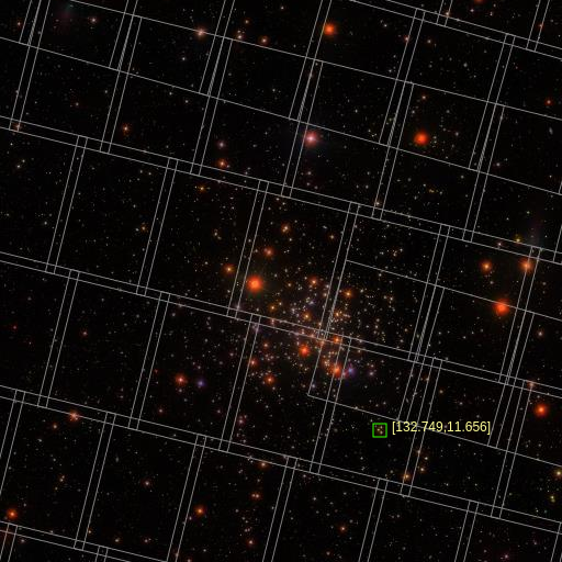
Figure 1: SDSS data highlighting image boundaries. Some images overlap substantially. Some light sources appear in multiple images that do not overlap. Celeste uses all relevant data to locate and characterize each light source whereas heuristics typically ignore all but one image in regions with overlap. Credit: SDSS DR10 Sky Navigate Tool.

II Background

Constructing an astronomical catalog is computationally demanding for any algorithm because of the sheer size of the datasets. Thus, approaches to date have been largely based on computationally efficient heuristics rather than Bayesian methods [4, 5]. Heuristics have a number of drawbacks: 1) they do not make optimal use of prior information because it is unclear how to “weight” it in relation to new information; 2)  they do not effectively combine knowledge from multiple image surveys, or even from multiple overlapping images from the same survey; and 3) they do not correctly quantify uncertainty of their estimates. They may flag some estimates as particularly unreliable, but confidence intervals follow only from a statistical model. Without modeling the arrival of photons as a Poisson process, for example, there is little basis for reasoning about uncertainty in the underlying brightness of light sources.

These shortcomings are addressed by the Bayesian formalism. An astronomical catalog’s entries are modeled as unobserved random variables with prior distributions. The posterior distribution encapsulates knowledge about the catalog’s entries, combining prior knowledge of astrophysics with new data from surveys in a statistically efficient manner; it represents the uncertainty. Because most light sources will be near the detection limit, these uncertainty estimates are as important as the parameter estimates themselves for many analyses.

Unfortunately, exact Bayesian posterior inference is NP-hard for most probabilistic models of interest [6]. Approximate Bayesian inference is an area of active research. Markov chain Monte Carlo (MCMC) is the most common approach. Unfortunately, the computational work required to draw enough “samples” makes it poorly suited to large-scale problems. It is also difficult to determine when the Markov chain has mixed.

To date, Tractor [7] is the only program for Bayesian posterior inference applied to a complete modern astronomical imaging survey. Tractor is a single-threaded program written in Python. It relies on Laplace approximation, in which the posterior is approximated with a multivariate Gaussian distribution centered at the mode, with the Hessian of the log likelihood function at the mode as its covariance matrix. This type of approximation is not suitable for categorical random variables, as no Gaussian distribution could approximate them well. Additionally, because Laplace approximation centers the Gaussian approximation at the mode rather than the mean, the solution depends heavily on the parameterization of the problem [6]. Nonetheless, Laplace approximation has been successfully applied to large-scale problems [8].

Variational inference (VI) extends Laplace approximation to approximate posterior distributions with non-Gaussian distributions. Like Laplace approximation, it uses numerical optimization to find a distribution that approximates the posterior without sampling [9]. In practice, the resulting optimization problem is often orders of magnitude faster to solve compared to MCMC approaches. Scaling VI to large datasets is nonetheless challenging. The largest published applications of VI to date have been to text mining, where topic models are fit to several gigabytes of text [10]. Modern astronomical datasets are at least four orders of magnitude larger than that.

Julia for HPC

To date, most HPC programs have been written in relatively verbose, low-level languages like C, C++, or Fortran. On the other hand, high-level languages’ expressiveness, feature-richness, and succinctness have motivated practitioners to develop techniques which mitigate their computational overhead. These techniques usually subscribe to Ousterhout’s two-language paradigm: one should use a systems programming language to write optimized kernels for performance “hot spots”, and use a scripting language to “glue” the kernels together and steer the overall computation [11]. NumPy [12] and PyFR [13] are examples of Ousterhout’s paradigm.

While the two-language approach has made leveraging high-level languages for HPC more feasible, it features a notable drawback: a sizable fraction of scientific computing projects begin with domain experts prototyping code in a high-level language, with the assumption that further in the development timeline, HPC experts will be able to identify performance bottlenecks and rewrite them into fast kernels by porting the code to a low-level language. Porting is time-consuming, expensive, error-prone, and can prevent rapid iteration between HPC experts and domain experts.

Julia is a high-level programming language that nonetheless lets programmers attain high performance. By leveraging just-in-time (JIT) compilation, multiple dispatch, type inference, and LLVM [14], Julia enables rapid, interactive prototyping while achieving performance competitive with C, C++, and Fortran [3]. Julia accomplishes this without forcing the programmer to use third-party “accelerators” (e.g. Numba, PyPy) or requiring hot kernels to be written in a low-level language.

Julia code is typically 5x to 10x shorter than code implementing the same functionality in C, C++, or Fortran. Computationally efficient Julia code is only slightly less succinct. Using a computationally efficient “StaticArray”, for example, is only slightly more verbose than a native (mutable) array. Moreover, even in an HPC codebase, the vast majority of the code accounts for little of the runtime. Here Julia is at least as succinct as Python.

III The Statistical Model

We adopt the probabilistic model from [15], which reports state-of-the-art scientific results but only scales inference to a several hundred stars and galaxies. The model is a joint probability distribution over observed random variables (the pixel intensities) and unobserved, or latent, random variables (the catalog entries). It is represented graphically in Figure 2.

For image $n=1,\ldots,N$, $\Lambda_{n}$ is a constant vector of metadata describing its sky location and the atmospheric conditions at the time of the exposure. Each pixel $m=1,\ldots,M$ in image $n$ has an intensity $x_{nm}$. This intensity is an observed random variable following a Poisson distribution with a rate parameter $F_{nm}$ unique to that pixel. $F_{nm}$ is a deterministic function of the catalog (which includes random quantities) and the image metadata. Pixel intensities are conditionally independent given the catalog.

For light source $s=1,\ldots,S$, the Bernoulli random variable $a_{s}$ indicates whether it is a star or a galaxy; a log-normal random variable $r_{s}$ denotes its brightness in a particular band of emissions (the “reference band”); and a multivariate normal random vector represents its colors—defined formally as the log ratio of brightnesses in adjacent bands, but corresponding to the colloquial definition of color. These random quantities have prior distributions with parameters $\Phi$, $\Upsilon$, and $\Xi$, respectively. These parameters are learned from preexisting astronomical catalogs. Additionally, each light source is characterized by unknown constant vectors $\mu_{s}$ and $\varphi_{s}$. The former indicates the light source’s location and the latter, if the light source is a galaxy, represents its shape, scale, and morphology. Though non-random, these vectors are nonetheless learned within our inference procedure.

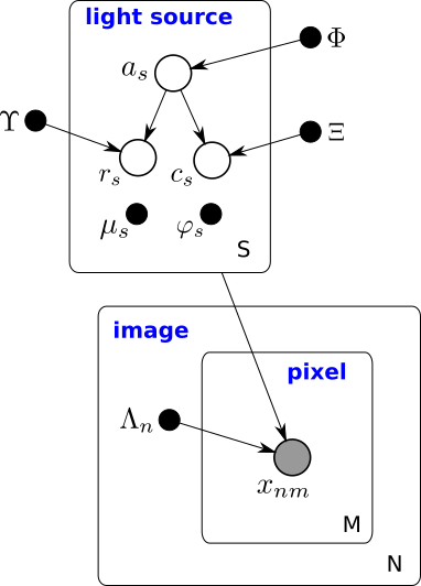
Figure 2: A graphical representation of the model we implement for astronomical images. Shaded vertices represent observed random variables. Empty vertices represent latent random variables. Black dots represent constants. Constants denoted by uppercase Greek characters are fixed throughout our procedure. Constants denoted by lowercase Greek letters are inferred, along with the posterior distribution of the latent random variables. Edges signify permitted conditional dependencies. The rounded rectangles represent independent replication.

Our primary use for the model is computing the distribution of its unobserved random variables conditional on a particular collection of astronomical images. This distribution is known as the posterior, and denoted $p(z|x)$, where $x:=\{x_{nm}\}_{n=1,m=1}^{N,M}$ represents all the pixels and $z:=\{a_{s},r_{s},c_{s}\}_{s=1}^{S}$ represents all the latent random variables. Exact posterior inference is computationally intractable for the proposed model, as it is for most non-trivial Bayesian models.

Variational inference (VI) finds an approximation to the posterior distribution $p(z|x)$ from a class of candidate distributions through numerical optimization [9]. The candidate approximating distributions $q_{\theta}$ are parameterized by a real-valued vector $\theta$. VI maximizes (with respect to $\theta$) the following lower bound on the log probability of the data:

$$\log p(x_{11},\ldots,x_{NM}) \geq\mathbb{E}_{q_{\theta}}\left[\log p(x,z)-\log q_{\theta}(z)\right]$$ (1)

$$=:\mathcal{L}(\theta).$$ (2)

This lower bound holds for any $q_{\theta}$, by Jensen’s inequality. We restrict $q_{\theta}$ to a class of distributions that let us evaluate the expectation in Equation 1 analytically. A complete description appears in [15].

To date, this approach to inference has only been applied to a small astronomical dataset containing 654 stars and galaxies [15]. In that work, numerical optimization is single-threaded, and light sources parameters are optimized in isolation, rather than jointly over the parameters for all the light sources. Joint optimization is a necessity for highly accurate scientific results.

IV Extreme scaling

Inferring an astronomical catalog for the SDSS dataset with the proposed statistical model amounts to solving a massive constrained optimization problem. Each of the 469 million celestial bodies has 44 parameters. Stored in double precision, the parameters alone are 154 GB. Moreover, each celestial body cannot be optimized in isolation: the optimal setting of its parameters depends on the optimal setting of nearby celestial bodies’ parameters, and vice versa. Yet the vast majority of pairs of celestial bodies can be optimized independently of each other (Figure 1).

Approaches to distributed optimization like HogWild [16] show that complicated locking mechanisms are not necessary to attain convergence to a stationary point. But those results apply only to stochastic gradient descent, which converges in sublinear time in theory and requires tens of thousands of iterations in practice. Newton’s method, on the other hand, converges quadratically in theory and in tens of iterations in practice, by leveraging second-order information. Because each iteration necessitates visiting a substantial fraction of the 55 TB dataset, exploiting second-order information is essential.

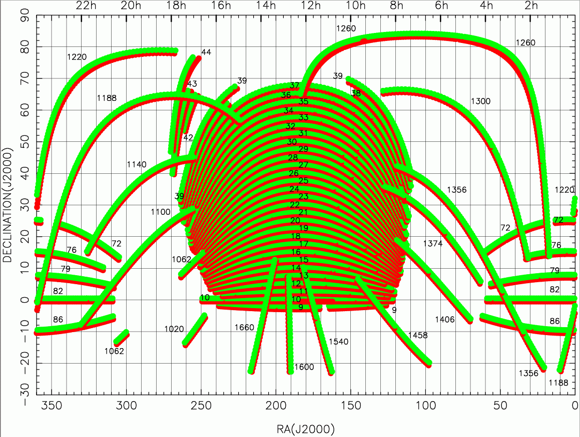
Figure 3: SDSS sky coverage map. Each monocolor arc (a “stripe”) represents the sky photographed during a particular night. The telescope remains fixed while the Earth rotates. Axes units are degrees of right ascension (RA) and declination (DEC) with respect to the equator. Credit: SDSS.

Our method has three levels: 1) non-overlapping rectangular regions of the sky are optimized concurrently on different nodes; 2) light sources within the same region of sky are optimized in parallel by different threads if they do not overlap and 3) individual light sources are optimized by a vectorized implementation of a variant of Newton’s method for nonconvex optimization. The outer- and mid-level of the optimization procedure correspond to block coordinate ascent, while the lowest level is second-order optimization. At each level, the parameters for light sources not optimized are held constant.

The description above explains why our optimizer converges, and gives some indication of how different routines align with the hardware. Now we give a more algorithmic description.

IV-A Task decomposition

The SDSS imaging camera scans the sky in stripes along “great circles” (Figure 3). Each stripe is divided into 12 MB image files that are stored on disk (Figure 1). Stripes overlap, and different stripes were scanned a differing number of times. To reason about a particular light source, all the images of it need to be loaded. The number varies significantly—between 5 and 480 images (up to 5.5 GB).

Most images contain hundreds or thousands of light sources. It is efficient to process multiple nearby light sources together on the same compute node so the images containing them just need to be loaded once for all of them, rather than once for each of them. Additionally, nearby light sources need to be optimized jointly. Optimizing them together on the same node allows for communication among threads through shared memory rather than over the network.

Therefore, we define our node-level tasks to correspond to contiguous regions of sky. Each task is to (jointly) find optimal parameters for the light sources in a particular region of the sky, with light sources in neighboring regions held fixed.

If our tasks correspond to large regions of sky, then most images that overlap with the region will lie entirely within it. That is desirable: the images on the boundary of a region typically overlap with another region too. We can minimize the mean number of times an image is loaded by specifying large tasks.

However, large tasks create inefficiencies both at the beginning and the end of a job. At the beginning of a job, the first task for each compute node cannot start processing until the image data is loaded. For subsequent tasks, the nodes can prefetch images before the previous task has completed, but not for the first task. At the end of a job, once the queue of unclaimed tasks is empty, some compute nodes will remain idle while others are still finishing their last task. We refer to this as load imbalance. If the tasks are long running, the load imbalance will be worse.

This poses a trade-off between effective load balance and image loading overhead. Smaller tasks allow for more effective load balance, but the same images must be loaded repeatedly. Larger tasks reduce the I/O burden, but simultaneously increase the load imbalance between processes.

It is not enough to partition the sky into uniformly sized regions, sized optimally to balance the trade-off between redundant image loading and load imbalance. No uniform size is good. Uniformly sized regions of the sky vary significantly in the number of light sources they contain, and the number of images of those light sources. Highly irregular task durations leads to high load imbalance.

Instead, we leverage an existing astronomical catalog to generate our tasks. We partition the sky recursively into regions that we expect to contain roughly the same number of bright pixels, based on existing astronomical catalogs. Bright pixels correlate with the amount of processing that will subsequently be needed. Task generation does not require loading image data, just an existing catalog, so we do it during preprocessing, as a one-off job, executed on a small number of nodes.

A task description also lists the light sources in the region to optimize subsequently, and gives initial values for these light sources’ parameters, derived from existing astronomical catalogs. Thus, it is an existing astronomical catalog that determines $S$, the total number of light sources in our statistical model. We may ultimately develop our own scripts for proposing candidate light sources for future datasets; for SDSS, however, existing catalogs work well for initializing our algorithm.

Tasks may be executed simultaneously: they consider non-overlapping regions of sky, so they are nearly independent in our objective function. However, light sources near a border of a region may not reach their optimal value if a neighboring region contains light sources that contribute photons to both region. For example, if a region contains a large, bright galaxy that extends beyond that region’s border, but that galaxy’s current parameters are not optimal, then the predictions in neighboring regions could also be off to compensate.

We address this by introducing a second stage to our algorithm—creating a second partitioning of the sky by shifting each region in the first partition by a fixed amount. Light sources near a border in the first partition will almost always away from a border in the second partition.

Each such partition constitutes a stage; tasks for the second stage are processed only after all tasks for the first stage are complete.

Task generation is the only stage of our algorithm completed during preprocessing. All other steps are part of the main job that we benchmark.

IV-B Task scheduling

Although we generate tasks to have roughly the same computational difficulty, their durations nonetheless vary too much for static scheduling. We use Dtree [17], a distributed dynamic scheduler that balances load for irregular tasks, even at petascale. Dtree organizes compute nodes into a tree whose height scales logarithmically in the number of nodes. To distribute tasks, each node only needs to communicate with its parent and its immediate children.

IV-C Shared state

During the optimization procedure, the current parameters for all celestial bodies are stored in a partitioned global address space (PGAS) [18]. Our interface mimics that of the Global Arrays Toolkit [19]. We use MPI-3 as the transport layer; get and put operations on elements make use of one-sided RMA operations that are supported in hardware on most supercomputer fabrics [20].

IV-D Task processing

Each node runs several multi-threaded processes. Each process receives a task for processing from the scheduler and performs some initialization steps—determining the relevant images to load as well as loading them from storage, fitting some image-specific parameters, and retrieving any previously computed parameters for light sources in the region. A typical task involves jointly optimizing roughly 500 light sources, each characterized by 44 parameters (about 20k parameters to optimize in total per task).

Multiple threads then coordinate to jointly optimize the light sources for the current task. They employ block coordinate ascent; each light source’s 44 parameters form a block. At each step of the algorithm, one light source’s parameters are optimized to machine tolerance by Newton’s method, with step sizes controlled by a trust region [21]. The trust region ensures convergence to a stationary point from any starting point even though the objective function is, in general, nonconvex.

Block coordinate ascent is a serial algorithm: if multiple overlapping blocks (of parameters) are updated in parallel the algorithm no longer converges in general. Instead, for a region of sky, threads coordinate their work through the Cyclades approach to conflict-free asynchronous machine learning [22]. Cyclades bases thread assignments on a “conflict graph.” Nodes are light sources and edges indicate a conflict. Light sources are in conflict if they overlap. Light sources that conflict cannot be optimized concurrently. At each iteration, Cyclades samples light sources at random without replacement and partitions the sample into connected components, according to the conflict graph restricted to the sample. Then, connected components are distributed among threads; lights sources that overlap in the sample are all assigned to the same thread. Cyclades works well because even if the conflict graph is connected, its restriction to a random sample of nodes typically has many connected components.

Each thread optimizes a particular light source’s parameters with any overlapping light sources’ parameters held fixed. By using Newton steps with exact Hessians rather than L-BFGS or a first-order optimization method, we attain a 1–2 order-of-magnitude speed-up. While L-BFGS is a robust and widely used optimization method, it struggles with the objective function for our problem, taking up to 2000 iterations to converge. Newton’s method, on the other hand, converges reliably on our problem in tens of iterations. Because the optimization problem is nonconvex, we also introduce a trust region constraint, as detailed in [21]. To apply Newton’s method, exact Hessians must be computed at each iteration. Each Hessian is a dense symmetric matrix with 44 rows and 44 columns. Computing the Hessian along with the gradient, rather than the gradient alone, takes 3x longer, but can reduce the total number of iterations by 100x relative to L-BFGS (which only requires gradients).

V PetaFLOP performance with Julia

Our implementation uses Julia’s multi-threading capabilities and Lisp-like macros, as well as external pure-Julia implementations of statically sized arrays [23]. Additionally, we use a Julia package for performing array-of-structs to struct-of-arrays conversion [24], enabling the compiler to replace certain expensive gather instructions with simple loads.

We also use automatic differentiation (AD), both forward-mode [25] and reverse-mode [26], but only where exploiting the sparsity of the Hessian is not required for good performance. While advanced sparsity-exploiting AD tools have been developed in Julia [27], these tools are either too experimental or restrictive for our use case. Instead, for performance-critical code, we use our own hand-coded derivatives that leverage custom index types to exploit Hessian sparsity structure.

During our final push toward attaining petascale performance, we made two types of changes: source-level refactoring of Celeste, and enhancements to the compiler in order to improve the quality of the generated instructions. For the former, Celeste’s code was refactored to reduce dynamic memory allocations, avoid dynamic method lookup, exploit sparsity patterns in matrix operations, ensure iteration order matched memory layout order, and reduce the memory footprint of per-pixel computations to fit almost entirely into L1 cache.

Additionally, we made three key improvements to Julia’s compiler. First, Julia’s ability to recognize and evaluate at compile time certain constant indexing computations was improved by increasing the precision of various analyses within type inference. Second, dereferenceability and automatic aliasing information was added to generated LLVM IR, augmented by user-provided code annotations and loop unrolling hints exposed as Julia macros. Third, LLVM compilation passes were improved by performing cost model adjustments, experimenting with pass order, and fixing instances where aliasing information was incorrectly discarded during compilation. Once these changes are officially incorporated upstream, they can benefit all Julia users and users of other LLVM frontends, such as the Clang C++ compiler.

With these improvements, the compiler’s vectorization and code generation capabilities—in particular, the fusion of multiplications and additions—allowed Celeste to obtain excellent code quality without resorting to low-level languages, assembly intrinsics, or handwritten libraries. Since most of these improvements were not target architecture specific, they yielded improvements not only on Celeste’s primary target architecture (Intel Xeon Phi), but also on other architectures (notably, Haswell).

VI Performance Measurement

VI-A System

We measure Celeste’s performance on the Cray XC40 Cori supercomputer (“Phase II”) at the National Energy Research Scientific Computing Center (NERSC). Cori Phase II contains 9688 compute nodes, each with one 1.40GHz 68-core Intel^® Xeon Phi^™ 7250 processor. Each core includes two AVX-512 vector processing units. Cores on a node connect through a two-dimensional mesh network with two cores per “tile.” Within a tile, cores share a 1 MB cache-coherent L2 cache.

Each node has 96 GB of DDR4 2400 MHz memory using six 16 GB DIMMs (115.2 GB/s peak bandwidth). Each node also includes 16 GB of on-package high-bandwidth memory with bandwidth five times that of DDR4 DRAM ($>460$ GB/sec). Cori’s high speed network is a Cray Aries high speed “dragonfly” topology interconnect.

Campaign data are stored on Cori’s 30 PB Lustre file system, with a theoretical aggregate bandwidth exceeding 700 GB/s. In addition, Cori features a Burst Buffer, a layer of non-volatile storage that sits between the processors’ memory and the parallel file system that serves to accelerate I/O performance of applications [28]. Cori includes 280 Burst Buffer nodes. Each of these contains two Intel P3608 3.2 TB NAND flash SSD modules attached over two PCIe gen3 interfaces. The Cori Burst Buffer provides approximately 1.7 TB/s of peak I/O performance with 28M IOPs, with 1.8 PB storage capacity.

VI-B Measurement methodology

All floating point operations (FLOPS) performed by Celeste are in double precision. The main source of FLOPS is evaluating the objective function and its gradient and Hessian. These evaluations’ FLOP counts are proportional to the number of active pixels. We use the Intel Software Development Emulator (SDE) to measure one and two active pixel visits and determined that each active pixel visit performs 32,317 FLOPS. We then count the number of active pixel visits during a run in order to measure total FLOPS.

The evaluation of the objective functions is the primary but not the only source of FLOPS. Other sources include the Newton trust region algorithm, as our implementation computes an eigen decomposition, as well as several Cholesky factorizations at each iteration. We again use SDE, this time for a larger multi-threaded run on a single node, and compare the flop count measured with the flop count derived from active pixel visits. We find that these additional sources of FLOPS increase the total flop count to 1.375 times the FLOP count derived from active pixel visits alone.

Thus, we determine the total number of FLOPS for Celeste by counting the number of active pixel visits during a run, and applying the 1.375 factor to account for FLOPS outside the objective function.

VII Performance Results

VII-A Per-thread analysis

Each thread’s runtime is 67% Julia generated code, 18% native dependencies such as image I/O libraries and the Julia runtime (memory allocation, thread management, etc.), 10% the system math library, 3% the Intel Math Kernel Library, and 2% the C standard library and the Linux kernel. Of all FLOPs, 82.3% operated on 8-wide AVX512 vector registers.

VII-B Per-node analysis

We empirically determined that eight threads per process and 17 processes per Intel Xeon Phi processor yields the highest throughput. Changing the number of threads and processes modifies memory access patterns in complicated ways as several factors are in tension: with more threads, several may remain idle at the end of a task while the last few light sources are optimized. With fewer threads, tasks take longer to complete, leading to more processes remaining idle while other processes finish their last task. An additional consideration is that threads share memory, whereas processes do not. Empirically, the 8x17 (threads x processes) node configuration does well at balancing all these considerations.

VII-C Multi-node scaling

We assess both weak and strong scaling with as many as 8192 nodes (557,056 CPU cores). The list of tasks is generated during preprocessing, as explained in Section IV-A. Every other step of our algorithm is measured as part of these scaling runs. We breakout runtimes into four components.

1. image loading – The time taken to load images while worker threads are idle. This time is accumulated by each process only for the first task. Images for subsequent tasks are prefetched.

2. load imbalance – All processes except the last one to finish accumulate load imbalance time after completing their last task; they are idle because the dynamic scheduler has no unassigned tasks left.

3. task processing – The main work loop, detailed in Section IV-D and profiled in section VII-A. This component involves no network or disk I/O: only computation and shared memory access. No time when threads are idle is included in this component.

4. other – Everything else, always a small fraction of the total runtime. This include scheduling overhead, all network I/O (excluding image loading), and writing output to disk.

For weak scaling, the problem size scales with the number of nodes, whereas for strong scaling, the problem size remains fixed. But how do we measure the size of a particular problem? If we double the square degrees of sky to process, we may end up increasing the problem difficulty by more or less than 2x: some regions are much more dense with bright light sources than others, or are imaged more times, as touched on in Section IV-A. It is tempting to consider just regions of sky that have roughly the same density of images, light sources, and bright light sources. But then our problem is not a single contiguous region of sky. Discontiguous regions have fewer dependencies between tasks, and these dependencies are of primary interest for multi-node scaling experiments.

Our solution is to treat the number of tasks, as determined by the preprocessing procedure in Section IV-A, as the size of the problem, and to use only contiguous regions of sky as problems. Tasks are recursively subdivided regions of sky that have roughly equal work. While runtimes for them can vary, that variation is an essential aspect of our approach, and thus something to preserve in our scaling runs.

For the largest scaling runs (139,264 processes), the size of our test dataset (SDSS) limits us to just four tasks per process. That gives the “image loading” component and the “load imbalance” components exaggerated importance. That does not limit the usefulness of the scaling results, but it needs to be accounted for when interpreting the scaling graphs.

VII-C1 Weak scaling

To assess weak scaling, we complete 68 tasks per node, or, equivalently, 4 tasks per process. Figure 4 shows runtimes for 1 node through 8192 nodes.

Task processing runtime is nearly constant throughout this range. This is expected since task processing is performed without communication.

Image loading time is also constant as the number of nodes grows—in part a testament to the hardware. Images are staged on an SSD array and accessed over the high speed interconnect described in Section VI-A.

Load imbalance comes to dominate runtime past 32 nodes (4352 threads), but this is more an artifact of the limited numbers of tasks (discussed above) than an issue with the approach. With just four tasks per process, its no scheduler could keep all the processes busy during a substantial fraction of the job. Nonetheless, the 8192 node run completes all 557,056 tasks in about 15 minutes, finding optimal parameters for 188,107,671 light sources.

Figure 4: Weak scaling. Runtime increases by 1.9X between 1 node (68 cores) and 8192 nodes (557,056 cores) while the number of tasks per node remains constant. See accompanying discussion of load imbalance.

VII-C2 Strong scaling

To evaluate strong scaling, we completed all 557,056 tasks with varying numbers of nodes. Figure 5 shows runtimes and their components at each scale. Image loading and task processing both exhibit near perfect scaling. “Other” remains constant as the node count grows, but remains a small fraction of overall runtime. Load imbalance grows in relative importance as the number of nodes increases. Particularly at high node counts, the degree of load imbalance reflects how few tasks are available per process. For all components, we observe 65% scaling efficiency from 2k to 4k nodes, and 50% efficiency from 2k to 8k nodes.

Figure 5: Strong scaling. See accompanying discussion of load imbalance.

VII-D Performance run

Processes are not synchronized and may be in different states at various points during a run—loading images, optimizing sources in a region of sky, or storing results. In order to determine the true peak performance that can be accomplished for Bayesian inference at scale, we prepared a specialized configuration for performance measurement in which the processes synchronize after loading images, prior to the optimization step. We then measure FLOPS performed across all processes by counting active pixel visits (Section VI-B) at one-minute intervals through the optimization step.

We ran this configuration on 9568 Cori Intel Xeon Phi nodes, each running 17 processes of eight threads each, for a total of 1,303,832 threads. 57.8 TB of image data was processed over a ten minute interval; the peak performance achieved was 1.54 PFLOP/s.

TABLE I: Sustained flop rate

	task processing	+load imbalance	+image loading
TFLOP/s	693.69	413.19	211.94

We report on sustained performance in Table I, using the standard Celeste configuration on 9600 nodes. This run completed 326,400 tasks in about seven minutes.

VIII Science results

We constructed an astronomical catalog for the entire 55 TB SDSS dataset. This catalog is the first fully Bayesian astronomical catalog for a modern astronomical imaging survey.

Absolute truth is unknowable for astronomical catalogs, but validation is nonetheless essential. One area of the sky (Stripe 82) has been imaged approximately 80 times in SDSS, whereas most regions have been imaged just once. This region provides a convenient validation strategy: combine exposures from all Stripe-82 runs to produce a very high signal-to-noise image, and estimate ground truth parameters from that image.

“Photo” [4] is a state-of-the-art software pipeline for constructing large astronomical catalogs. Photo is a carefully hand-tuned heuristic. We use Photo’s estimated parameters from the combined Stripe 82 imagery as ground truth. We then compare Photo’s output for a single run’s imagery to Celeste’s output for the same images. Although this “ground truth” is still prone to errors, such errors typically favor Photo, since any systematic errors will be consistent in Photo’s output.

In addition to point estimates, Celeste offers measures of posterior uncertainty for source type (star or galaxy), brightness, and colors. This is a novel feature owing to Celeste’s formulation as a Bayesian model, offering astronomers a principled measure of the quality of inference for each light source. No such analogue exists for Photo.

TABLE II: Average error based on light sources from Stripe 82.

	Photo	Celeste
Position	0.36	0.27
Missed gals	0.06	0.19
Missed stars	0.12	0.15
Brightness	0.21	0.14
Color u-g	1.32	0.60
Color g-r	0.48	0.21
Color r-i	0.25	0.12
Color i-z	0.48	0.17
Profile	0.38	0.28
Eccentricity	0.31	0.23
Scale	1.62	0.92
Angle	22.54	17.54

Lower is better. Results in bold are better by more than two standard deviations. “Position” is error, in pixels, for the location of the light sources’ centers. “Missed gals” is the proportion of galaxies labeled as stars. “Missed stars” is the proportion of stars labeled as galaxies. “Brightness” measures the reference band (r-band) magnitude. “Colors” are ratios of magnitudes in consecutive bands. “Profile” is a proportion indicating whether a galaxy is de Vaucouleurs or exponential. “Eccentricity” is the ratio between the lengths of a galaxy’s minor and major axes. “Scale” is the effective radius of a galaxy in pixels. “Angle” is the orientation of a galaxy in degrees.

The first numeric column of Table II shows error on each parameter from Photo, averaged over all sources in the chosen image. The second numeric column shows results for Celeste. Celeste achieves improved accuracy on nearly all estimated parameters, usually by a substantial margin, improvements that are both statistically significant and of practical significance to astronomers. Photo outperforms Celeste only at classifying galaxies. Upon manual inspection, the true class of these mislabeled light sources often seem to be genuinely ambiguous. Some may be quasars, which are collapsing galaxies with point-like spatial characteristics of stars. Celeste’s posterior uncertainty reflects the ambiguity.

IX Discussion

IX-A Bayesian inference and distributed optimization

Our work demonstrates conclusively that massive, complex datasets can be analyzed with Bayesian inference. It is not necessary to resort to a heuristic when Bayesian inference is preferable, or to settle for recovering just the mode of the posterior. Through a combination of algorithmic techniques that were previously unexplored for variational inference, and a careful implementation, high throughput is possible.

Distributed optimization is important for variational inference, as well as for optimization problems that do not arise from statistical models. The multi-level approach we propose is well-suited to HPC numerical optimization because it utilizes all available levels of parallelism. It has only modest communication requirements, yet converges in few iterations to a stationary point.

IX-B Convergence of high-productivity languages and high-performance languages

Celeste constitutes the first successful use of Julia at petascale, demonstrating Julia’s viability for HPC applications where performance constraints would have otherwise demanded the use of a low-level language like C or Fortran. Our experience challenges the traditional HPC wisdom that interactive, high-level languages are unsuitable for performance hot spots, and instead must be limited to a “glue” role, such that the majority of an application’s runtime is spent in low-level kernels.

Julia may not always be preferable to a traditional HPC workflow—legacy code, existing libraries, and the time required to learn a new language are all good reasons why C and Fortran will remain popular for HPC. But the reasons why Julia worked well for Celeste seem far from unique to our project. New HPC projects—particularly those planning to write prototype code and production code in different languages—may benefit from using Julia instead.

References

- [1] S. Alam, F. D. Albareti et al., “The eleventh and twelfth data releases of the sloan digital sky survey: Final data from SDSS-III,” The Astrophysical Journal Supplement Series, vol. 219, no. 1, p. 12, 2015.
- [2] Large Synoptic Survey Telescope Consortium, “About LSST,” http://www.lsst.org/about, 2017, [Online; accessed September 12, 2017].
- [3] J. Bezanson, A. Edelman, S. Karpinski, and V. B. Shah, “Julia: A fresh approach to numerical computing,” SIAM Review, vol. 59, no. 1, pp. 65–98, 2017.
- [4] R. H. Lupton, Z. Ivezic et al., “SDSS image processing II: The photo pipelines,” Technical report, Princeton University, Tech. Rep., 2005.
- [5] E. Bertin and S. Arnouts, “SExtractor: Software for source extraction,” Astronomy and Astrophysics Supplement Series, vol. 117, no. 2, pp. 393–404, 1996.
- [6] C. M. Bishop, Pattern Recognition and Machine Learning. Springer, 2006.
- [7] D. Lang, “The Tractor,” http://thetractor.org/about/, 2017, [Online; accessed October 22, 2017].
- [8] A. Alexanderian, N. Petra, G. Stadler, and O. Ghattas, “A fast and scalable method for A-optimal design of experiments for infinite-dimensional Bayesian nonlinear inverse problems,” SIAM Journal on Scientific Computing, vol. 38, no. 1, pp. A243–A272, 2016.
- [9] D. M. Blei, A. Kucukelbir, and J. D. McAuliffe, “Variational inference: A review for statisticians,” Journal of the American Statistical Association, 2017.
- [10] M. D. Hoffman, D. M. Blei, C. Wang, and J. W. Paisley, “Stochastic variational inference.” Journal of Machine Learning Research, vol. 14, no. 1, pp. 1303–1347, 2013.
- [11] J. K. Ousterhout, “Scripting: Higher level programming for the 21st century,” Computer, vol. 31, no. 3, pp. 23–30, 1998.
- [12] S. v. d. Walt, S. C. Colbert, and G. Varoquaux, “The NumPy array: A structure for efficient numerical computation,” Computing in Science & Engineering, vol. 13, no. 2, pp. 22–30, 2011.
- [13] P. Vincent, F. Witherden, B. Vermeire, J. S. Park, and A. Iyer, “Towards green aviation with python at petascale,” in Proceedings of the International Conference for High Performance Computing, Networking, Storage and Analysis, ser. SC’16, 2016.
- [14] C. Lattner and V. Adve, “LLVM: A compilation framework for lifelong program analysis & transformation,” in Proceedings of the International Symposium on Code Generation and Optimization. IEEE Computer Society, 2004, p. 75.
- [15] J. Regier, A. Miller, J. McAuliffe, R. Adams, M. Hoffman, D. Lang, D. Schlegel, and Prabhat, “Celeste: Variational inference for a generative model of astronomical images,” in Proceedings of the 32nd International Conference on Machine Learning, 2015.
- [16] B. Recht, C. Re, S. Wright, and F. Niu, “Hogwild: A lock-free approach to parallelizing stochastic gradient descent,” in Advances in Neural Information Processing Systems, 2011.
- [17] K. Pamnany, S. Misra, V. Md, X. Liu, E. Chow, and S. Aluru, “Dtree: Dynamic task scheduling at petascale,” in International Conference on High Performance Computing. Springer, 2015, pp. 122–138.
- [18] Tim Stitt, “An introduction to the partitioned global address space programming model.”
- [19] J. Nieplocha, B. Palmer, V. Tipparaju, M. Krishnan, H. Trease, and E. Aprà, “Advances, applications and performance of the Global Arrays Shared Memory Programming Toolkit,” International Journal of High Performance Computing Applications, vol. 20, no. 2, pp. 203–231, 2006.
- [20] T. Hoefler, J. Dinan, R. Thakur, B. Barrett, P. Balaji, W. Gropp, and K. Underwood, “Remote memory access programming in MPI-3,” ACM Trans. Parallel Comput., vol. 2, no. 2, pp. 9:1–9:26, Jun. 2015.
- [21] S. Wright and J. Nocedal, “Numerical optimization,” Springer Science, vol. 35, pp. 67–68, 1999.
- [22] X. Pan, M. Lam, S. Tu, D. Papailiopoulos, C. Zhang, M. I. Jordan, K. Ramchandran, and C. Ré, “Cyclades: Conflict-free asynchronous machine learning,” in Advances in Neural Information Processing Systems, 2016.
- [23] Andy Ferris, “StaticArrays.jl,” https://github.com/JuliaArrays/StaticArrays.jl, 2017, [Online; accessed October 22, 2017].
- [24] Simon Kornblith, “StructsOfArrays.jl,” https://github.com/simonster/StructsOfArrays.jl, 2017, [Online; accessed September 12, 2017].
- [25] J. Revels, M. Lubin, and T. Papamarkou, “Forward-mode automatic differentiation in Julia,” in Proceedings of the 7th International Conference on Algorithmic Differentiation, 2016.
- [26] Jarrett Revels, “ReverseDiff.jl,” https://github.com/JuliaDiff/ReverseDiff.jl, 2017, [Online; accessed September 12, 2017].
- [27] F. Qiang, C. Petra, M. Lubin, J. Huchette, and M. Anitescu, “On efficient Hessian computation using the edge pushing algorithm in Julia,” in Proceedings of the 7th International Conference on Algorithmic Differentiation, 2016.
- [28] W. Bhimji, D. Bard, M. Romanus, D. Paul et al., “Accelerating science with the NERSC Burst Buffer Early User Program,” Cray User Group 2016 Proceedings, 2016.