Sums with the Möbius function twisted
by characters with powerful moduli

Abstract.

In their recent work, the authors (2016) have combined classical ideas of A. G. Postnikov (1956) and N. M. Korobov (1974) to derive improved bounds on short character sums for certain nonprincipal characters with powerful moduli. In the present paper, these results are used to bound sums of the Möbius function twisted by characters of the same type, complementing and improving some earlier work of B. Green (2012). To achieve this, we obtain a series of results about the size and zero-free region of $L$-functions with the same class of moduli.

1. Introduction

Our work in this paper is motivated, in part, by a program of Sarnak [12] to establish instances of a general pseudo-randomness principle related to a famous conjecture of Chowla [3]. Roughly speaking, the principle asserts that the Möbius function $\mu$ does not correlate with any function $F$ of low complexity, so that

$$\sum_{n\leqslant x}\mu(n)F(n)=o\left(\sum_{n\leqslant x}|F(n)|\right)\qquad(x\to\infty).$$ (1.1)

Combining a result of Linial, Mansour and Nisan [10] with techniques of Harman and Kátai [6], Green [5] has shown that if $F:\{0,\ldots,N-1\}\to\{\pm 1\}$ has the property that $F(n)$ can be computed from the binary digits of $n$ using a bounded depth circuit, then $F$ is orthogonal to the Möbius function $\mu$ in the sense that (1.1) holds; see [5, Theorem 1.1]. Among other things, Green’s proof [5] relies on a bound for a sum with the Möbius function twisted by a Dirichlet character $\chi$ of modulus $q=2^{\gamma}$. To formulate the result of [5] we denote

$$M(x,\chi)=\sum_{n\leqslant x}\mu(n)\chi(n),$$ (1.2)

where $\chi$ is a Dirichlet character modulo $q$; we refer the reader to [9, Chapter 3] for the relevant background on characters. We also denote

$$\widehat{M}_{q}(x)=\max_{\chi\bmod q}|M(x,\chi)|,$$ (1.3)

where the maximum is taken over all Dirichlet characters $\chi$ modulo $q$. We remark that although the principal character $\chi_{0}$ is included in the definition (1.3), the pure sum $M(x,\chi_{0})$ plays no rôle as it satisfies a stronger bound than any bounds currently known for $M(x,\chi)$, $\chi\neq\chi_{0}$; see [14, Chapter V, Section 5, Equation (12)] (and also [13] for the best known bound under the Riemann Hypothesis).

According to [5, Theorem 4.1], for some absolute constant $c_{1}>0$ and all moduli of the form

$$q=2^{\gamma}\leqslant e^{c_{1}\sqrt{\log x}},$$ (1.4)

the bound

$$\widehat{M}_{q}(x)=O\left(xe^{-c_{1}\sqrt{\log x}}\right)$$ (1.5)

holds, where the implied constant is absolute.

Our aim in the present paper is to improve this result in the three directions. Namely, we obtain a new bound which is

• stronger than (1.5) and gives a better saving with a higher power of $\log x$ in the exponent;

• valid for a larger class of moduli $q$;

• nontrivial in a broader range of the parameters $q$ and $x$.

As immediate applications, our new bounds yield improvements of some other results of Green [5].

To achieve this aim, we derive a series of new results concerning the size and zero-free region of $L$-functions and their derivatives with the same class of moduli, which we believe can be of independent interest and have other applications.

2. Main result

For any functions $f$ and $g$, the notations $f(x)\ll g(x)$, $g(x)\gg f(x)$ and $f(x)=O(g(x))$ are used interchangeably to mean that $|f(x)|\leqslant c|g(x)|$ holds with some constant $c>0$. Throughout the paper, we indicate explicitly any parameters on which the implied constants may depend.

Given a natural number $q$, its core (or kernel) is the product $\mathfrak{q}_{\sharp}$ over the prime divisors $p$ of $q$; that is,

$$\mathfrak{q}_{\sharp}=\prod_{p\mid q}p.$$

In this paper, we are mainly interested in bounding the sums $M(x,\chi)$ for certain moduli $q$ that have a suitable core $\mathfrak{q}_{\sharp}$. Specifically, we assume that

$$\min\limits_{p\mid q}\{v_{p}(q)\}\geqslant 0.7\gamma\qquad\text{with}\quad\gamma=\max\limits_{p\mid q}\{v_{p}(q)\}\geqslant\gamma_{0},$$ (2.1)

where $\gamma_{0}>0$ is a sufficiently large absolute constant, and $v_{p}$ denotes the standard $p$-adic valuation (that is, for $n\neq 0$ we have $v_{p}(n)=\alpha$, where $\alpha$ is the largest integer such that $p^{\alpha}\mid n$). The technical condition (2.1) is needed in order to apply the results of our earlier paper [1]; it is likely that this constraint can be modified and relaxed in various ways.

Remark 2.1.

Our work in the present paper (and earlier in [1]) is motivated by applications in the important special case that $q=p^{\gamma}$ is a prime power. In this situation, the failure of the condition (2.1) simply means that $q=O(1)$, and in this case there are usually results in the literature which are superior to ours. For example, we use this observation to derive Corollary 3.1 below. ∎

In addition to (1.2) we consider sums of the form

$$\psi(x,\chi)=\sum_{n\leqslant x}\Lambda(n)\chi(n),$$ (2.2)

where $\Lambda$ is the von Mangoldt function; such sums are classical objects of study in analytic number theory (see, e.g., [9, Section 5.9] or [11, Section 11.3]). We expect that the techniques of this paper can be applied to bound other sums of number theoretic interest.

We treat the sums $M(x,\chi)$ and $\psi(x,\chi)$ in parallel. Building on the results and techniques of [1] we derive the strongest bounds currently known for such sums when the modulus $q$ of $\chi$ satisfies (2.1). In particular, we improve and generalize Green’s bound (1.5). Moreover, we obtain nontrivial bounds assuming only that

$$q\leqslant\exp\left(c_{1}(\log x)^{3/2}(\log\log x)^{-7/2}\right)$$ (2.3)

holds rather than (1.4) (that is, our results are nontrivial for shorter sums).

Theorem 2.2.

Let $q$ be a modulus satisfying (2.1). There is a constant $c>0$ that depends only on $\mathfrak{q}_{\sharp}$ and has the following property. Let

$$Q_{1} =\exp\left((\log q)^{7/3}(\log\log q)^{5/3}\right),$$

$$Q_{2} =\exp\left((\log q)^{7}(\log\log q)^{-1}\right),$$

and for $j=1,2$ put

$$E_{j}=\begin{cases}\exp\left(-c\log x\cdot(\log q)^{-2/3}(\log\log q)^{-4/3}\right)\cdot(\log x)^{j}&\quad\hbox{if $x\leqslant Q_{1}$},\\ \exp\left(-c(\log x\cdot\log q)^{1/2}(\log\log q)^{-1/2}\right)&\quad\hbox{if $Q_{1}<x\leqslant Q_{2}$},\\ \exp\left(-c(\log x)^{4/7}(\log\log x)^{-3/7}\right)&\quad\hbox{if $x>Q_{2}$}.\end{cases}$$

For every primitive character $\chi$ modulo $q$ we have

$$\frac{1}{x}M(x,\chi)\ll E_{1}\qquad\mbox{and}\qquad\frac{1}{x}\psi(x,\chi)\ll E_{2}.$$

We remark that Green’s bound (1.5) applies to arbitrary characters whereas Theorem 2.2 is formulated only for primitive characters. However, in the special case that $q=2^{\gamma}$, the conductor $q_{0}$ of an arbitrary Dirichlet character $\chi$ modulo $q$ is a power of two (since $q_{0}\mid q$), and $\chi$ is a primitive character modulo $q_{0}$. When $q_{0}\geqslant 2^{\gamma_{0}}$ we still apply Theorem 2.2 with $q_{0}$ in place of $q$, and this only increases the range (2.3) in which we have a nontrivial bound.

We now give a simpler formulation of Theorem 2.2 in the regime

$$q=\exp\left((\log x)^{\alpha+o(1)}\right),$$ (2.4)

where $\alpha>0$ is a fixed real parameter.

Corollary 2.3.

Let $\alpha>0$ be fixed, let $q$ be a modulus satisfying (2.1), and suppose that (2.4) holds. For every primitive character $\chi$ modulo $q$ we have

$$\max\{|M(x,\chi)|,|\psi(x,\chi)|\}\leqslant x\exp\left(-(\log x)^{\beta(\alpha)+o(1)}\right),$$

where

$$\beta(\alpha)=\begin{cases}4/7&\quad\hbox{if $\alpha\leqslant 1/7$},\\ (1+\alpha)/2&\quad\hbox{if $1/7\leqslant\alpha\leqslant 3/7$},\\ 1-2\alpha/3&\quad\hbox{if $\alpha\geqslant 3/7$}.\end{cases}$$

Alternatively, we can define the function $\beta(\alpha)$ of Corollary 2.3 by

$$\beta(\alpha)=\min\left\{\max\left\{4/7,(1+\alpha)/2\right\},1-2\alpha/3\right\};$$

see also Figure 2.1 for its behavior.

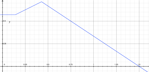
Figure 2.1. Function $\beta(\alpha)$

Our proof of Theorem 2.2 is based on new bounds on Dirichlet polynomials and on the magnitudes and zero-free regions of certain $L$-functions, which extend and improve those of Gallagher [4], Iwaniec [8] and the authors [1]; see Section 4 for more details. We believe these bounds are of independent interest and may have many other arithmetic applications. In particular, one can apply these results to estimate character sums and exponential sums twisted by the Liouville function, the divisor function, and other functions of number theoretic interest.

3. Applications

It is easy to see that Theorem 2.2 improves Green’s result [5, Theorem 4.1] in terms of both the range, increasing the right hand side in (1.4), and the strength of the bound, reducing the right hand side in (1.5). Although one can derive a general result with a trade-off between the range and the strength of the bound, we present only two special cases:

• Improving the range (1.4) as much as possible while preserving (1.5);

• Improving the bound (1.5) as much as possible (in this case, we are able to improve the range as well).

More precisely, for $(i)$ we note that the first bound of Theorem 2.2 implies that

$$\log\left(x^{-1}|M(x,\chi)|\right)\ll\sqrt{\log x}$$ (3.1)

holds for a character $\chi$ modulo $q=2^{\gamma}$ provided that $\log q\ll(\log x)^{3/4}(\log\log x)^{-2}$ and the conductor of $\chi$ satisfies $q_{0}\geqslant 2^{\gamma_{0}}$ (so Theorem 2.2 applies). Since the remaining characters $\chi$ modulo $q$ that have $q_{0}<2^{\gamma_{0}}$ comprise a finite set, the bound (3.1) can be achieved for those characters on a one-to-one basis; see, e.g., the paper of Hinz [7] and references therein. Using (3.1) to bound $\widehat{M}_{q}(x)$ we derive the following statement.

Corollary 3.1.

For some absolute constant $c_{1}>0$ and all moduli of the form

$$q=2^{\gamma}\leqslant e^{c_{1}(\log x)^{3/4}(\log\log x)^{-2}}\qquad(\gamma\in\mathbb{N})$$

the bound (1.5) holds.

Similarly, for $(ii)$ we take $q$ smaller than in Corollary 3.1 so the last two bounds in definition of $E_{1}$ in Theorem 2.2 dominate. We obtain the following statement.

Corollary 3.2.

For some absolute constant $c_{1}>0$ and all moduli of the form

$$q=2^{\gamma}\leqslant e^{c_{1}(\log x)^{9/14}(\log\log x)^{-19/14}}\qquad(\gamma\in\mathbb{N})$$

the bound

$$\widehat{M}_{q}(x)\ll xe^{-c_{1}(\log x)^{4/7}(\log\log x)^{-3/7}}$$

holds.

Notice that the exponents $3/4$ and $9/14$ that occur in Corollaries 3.1 and 3.2 are the maximal roots $\alpha$ of the equations $\beta(\alpha)=1/2$ and $\beta(\alpha)=4/7$, respectively (in Figure 2.1 these roots occur at the rightmost intersection points between the graph of $\beta(\alpha)$ and the horizontal lines at height $1/2$ and $4/7$, respectively).

We also remark that Corollaries 3.1 and 3.2 hold with $2^{\gamma}$ replaced by $p^{\gamma}$ for any fixed prime $p$; in this case, the constant $c_{1}>0$ can depend on $p$ but is otherwise absolute.

Next, we turn our attention to the following exponential sums twisted by the Möbius function:

$$S_{q}(x,a)=\sum_{n\leqslant x}\mu(n)\exp(2\pi ian/q)\qquad(a\in\mathbb{Z}).$$

We denote

$$\widehat{S}_{q}(x)=\max_{a\in\mathbb{Z}}\left|S_{q}(x,a)\right|.$$

Green has shown (see [5, Corollary 4.2]) that for some absolute constant $c_{2}>0$ and all moduli of the form

$$q=2^{\gamma}\leqslant e^{c_{2}\sqrt{\log x}},$$

the bound

$$\widehat{S}_{q}(x)\ll xe^{-c_{2}\sqrt{\log x}}$$

holds. The proof is obtained by relating $\widehat{S}_{q}(x)$ to $\widehat{M}_{q}(x)$ and then exploiting the bound (1.5). In order to get a nontrivial bound on $\widehat{S}_{q}(x)$ in this way, the savings in the bound on $\widehat{M}_{q}(x)$ has to be a little larger than $q$. For this reason, even though Corollaries 3.1 and 3.2 are suitable for such applications (and lead to an improvement of [5, Corollary 4.2] in both the range and strength of the bound), we need to slightly reduce the range of $q$. Furthermore, a full analogue of these results also holds for sums with the Möbius function in arithmetic progressions; that is, we can bound the quantity

$$\widehat{D}_{q}(x)=\max_{\begin{subarray}{c}a\in\mathbb{Z}\\ \gcd(a,q)=1\end{subarray}}\left|D_{q}(x,a)\right|,$$

where

$$D_{q}(x,a)=\sum_{\begin{subarray}{c}n\leqslant x\\ n\equiv a\bmod q\end{subarray}}\mu(n).$$

Corollary 3.3.

For some absolute constant $c_{2}>0$ and all moduli of the form

$$q=2^{\gamma}\leqslant e^{c_{2}(\log x)^{3/5}(\log\log x)^{-4/5}}\qquad(\gamma\in\mathbb{N})$$

we have

$$\max\{\widehat{S}_{q}(x),\widehat{D}_{q}(x)\}\ll xe^{-c_{2}(\log x)^{4/7}(\log\log x)^{-3/7}}.$$

Note that the exponent $3/5$ in Corollary 3.3 is the root $\alpha$ of the equation $\beta(\alpha)=\alpha$, and we have

$$\min\left\{\beta(\alpha):\alpha\in(0,3/5]\right\}=4/7.$$

As with the previous results, Corollary 3.3 also holds with $2^{\gamma}$ replaced by $p^{\gamma}$ for any fixed prime $p$.

Finally, we mention that the results of the present paper can be used to estimate Fourier-Walsh coefficients $\widehat{\mu}_{n}(\mathcal{A})$ associated with the Möbius function, interpolating between the result of Green [5, Proposition 1.2] and that of Bourgain [2, Theorem 1]. Recall that for a natural number $n$ and a set $\mathcal{A}\in\{0,\ldots,n-1\}$, the coefficient $\widehat{\mu}_{n}(\mathcal{A})$ is defined by

$$\widehat{\mu}_{n}(\mathcal{A})=\sum_{(x_{0},\ldots,x_{n-1})\in\{0,1\}^{n}}\prod_{j\in\mathcal{A}}(1-2x_{j})\mu\left(\sum_{j=0}^{n-1}2^{j}x_{j}\right).$$

Green [5, Proposition 1.2] uses (1.5) to give a nontrivial bound on $\widehat{\mu}_{n}(\mathcal{A})$ for sets $\mathcal{A}$ of cardinality $|\mathcal{A}|\ll n^{1/2}/\log n$, and this bound on the cardinality is essential the entire approach of [5]. Bourgain [2, Theorem 1] gives a nontrivial bound on $\widehat{\mu}_{n}(\mathcal{A})$ for arbitrary sets. Using Theorem 2.2 in the argument of Green [5] one can obtain a result that is stronger than [5, Proposition 1.2] but which also holds for larger sets.

4. Outline of the proof

To prove Theorem 2.2, we begin by extending the bound of [1, Theorem 2.2] to cover Dirichlet polynomials supported on shorter intervals; see Theorem 5.1. Adapting various ideas and tools from [1] to exploit this result on Dirichlet polynomials, we give a strong bound on the size of the relevant $L$-functions $L(s,\chi)$ in the case that $\Im(s)$ is not too large; see Theorem 6.2. For larger values of $\Im(s)$, we apply a well known bound of Iwaniec [8, Lemma 8].

Having the upper bounds on these $L$-functions at our disposal, we combine them with certain results and ideas of [1] and [8] to obtain a new zero-free region, which is wider than all previously known regions; see Theorem 7.2.

Next, we introduce and apply an extension of a result of Montgomery and Vaughan [11, Lemma 6.3] which bounds the logarithmic derivative of a complex function in terms of its zeros; see Lemma 8.1. Similarly to [11], we use Lemma 8.1 as a device that allows us to consolidate old and new bounds on the size and the zero-free region of our $L$-functions $L(s,\chi)$, and doing so leads us to Theorem 8.4, which provides strong bounds on these $L$-functions, their logarithmic derivatives, and their reciprocals.

Finally, to conclude the proof of Theorem 2.2, in Section 9 we relate (via Perron’s formula) the sums $M(x,\chi)$ and $\psi(x,\chi)$ to the bounds given in Theorem 8.4. This connection involves the use of a parameter $T$, which we optimise to achieve the desired result. It is worth mentioning that the final optimisation step is somewhat delicate since our bounds behave very differently in different ranges (e.g., see (8.5)).

5. Bounds on Dirichlet polynomials

In this section, we study Dirichlet polynomials of the form

$$T_{\chi}(M,N;t)=\sum_{M<n\leqslant M+N}\chi(n)n^{it}\qquad(t\in\mathbb{R}).$$

As in [1], to bound these polynomials we approximate each $T_{\chi}(M,N;t)$ with a sum of the form

$$\sum_{M<n\leqslant M+N}\chi(n)\mathrm{e}(G(n)),$$

where $G$ is a polynomial with real coefficients, and $\mathrm{e}(t)=e^{2\pi it}$ for all $t\in\mathbb{R}$. Our result is the following statement, which is more flexible than [1, Theorem 2.2].

Theorem 5.1.

For every $C>1$ there are effectively computable constants $\gamma_{0},\xi_{0}>0$ depending only on $C$ such that the following property holds. For any modulus $q$ satisfying (2.1) and any primitive character $\chi$ modulo $q$, the bound

$$T_{\chi}(M,N;t)\ll N^{1-\xi_{0}/\varrho^{2}}$$ (5.1)

holds uniformly for all $M,N,t\in\mathbb{R}$ subject to the conditions

$$M\geqslant N,\qquad\mathfrak{q}_{\sharp}^{\gamma_{0}}\leqslant N\leqslant q^{C}\qquad\mbox{and}\qquad|t|\leqslant q^{\frac{1}{4}(\log M)/\log\mathfrak{q}_{\sharp}},$$ (5.2)

where $\varrho=(\log q)/\log N$ and implied constant in (5.1) depends only on $C$.

Proof.

Let $\gamma_{0}$ be a positive constant exceeding $e^{200}$, and put

$$\gamma_{1}=\frac{\log N}{\log\mathfrak{q}_{\sharp}}\qquad\mbox{and}\qquad\varepsilon=\frac{5}{4\gamma_{1}}=\frac{5\log\mathfrak{q}_{\sharp}}{4\log N}.$$

Using (2.1) and (5.2) we have

$$\log q=\sum_{p\mid q}v_{p}(q)\log p\leqslant\gamma\sum_{p\mid q}\log p=\gamma\log\mathfrak{q}_{\sharp}\leqslant\gamma\gamma_{1}^{-1}\log N,$$

hence $\varrho$ lies in $[C^{-1},\gamma/\gamma_{1}]$. Let $s=\left\lfloor\varepsilon\gamma/\varrho\right\rfloor$. Since $\varepsilon\gamma/\varrho\geqslant\varepsilon\gamma_{1}=\frac{5}{4}$ we have

$$\tfrac{1}{5}\varepsilon\gamma/\varrho\leqslant\varepsilon\gamma/\varrho-1<s\leqslant\varepsilon\gamma/\varrho,$$ (5.3)

and therefore $s\asymp\gamma/\varrho$.

Now let $\nu=\left\lceil\gamma/(3s)\right\rceil$. For any real number $x$, we have the estimate

$$(1+x)^{it}=\mathrm{e}(tG(x))\left(1+O(|t||x|^{\nu})\right),$$

where $G$ is the polynomial given by

$$G(x)=\frac{1}{2\pi}\sum_{r=1}^{\nu-1}(-1)^{r-1}\frac{x^{r}}{r}.$$

Hence, uniformly for $n\in[M+1,M+N]$ and $y,z\in[1,\mathfrak{q}_{\sharp}^{s}]$, taking into account that $M\geqslant N$, we have

$$\left(n+\mathfrak{q}_{\sharp}^{s}yz\right)^{it}=n^{it}(1+\mathfrak{q}_{\sharp}^{s}yz/n)^{it}=n^{it}\mathrm{e}(tG(\mathfrak{q}_{\sharp}^{s}yz/n))+O(M^{-\nu}|t|\mathfrak{q}_{\sharp}^{3s\nu}).$$ (5.4)

Let $\mathcal{N}$ be the set of integers coprime to $q$ in the interval $[M+1,M+N]$. Shifting the interval $[M+1,M+N]$ by the amount $\mathfrak{q}_{\sharp}^{s}yz$, where $1\leqslant y,z\leqslant\mathfrak{q}_{\sharp}^{s}$, we have the uniform estimate

$$T_{\chi}(M,N;t) =\sum_{n\in\mathcal{N}}\chi(n)n^{it}$$

$$=\sum_{n\in\mathcal{N}}\chi(n+\mathfrak{q}_{\sharp}^{s}yz)(n+\mathfrak{q}_{\sharp}^{s}yz)^{it}+O(\mathfrak{q}_{\sharp}^{3s}).$$

Using (5.4) and averaging over all such $y$ and $z$, it follows that

$$T_{\chi}(M,N;t)=\mathfrak{q}_{\sharp}^{-2s}V+O(\mathfrak{q}_{\sharp}^{3s}+NM^{-\nu}|t|\mathfrak{q}_{\sharp}^{3s\nu}),$$

where

$$V=\sum_{n\in\mathcal{N}}\chi(n)n^{it}\sum_{y,z=1}^{\mathfrak{q}_{\sharp}^{s}}\chi(1+\mathfrak{q}_{\sharp}^{s}\overline{n}yz)\mathrm{e}(tG(\mathfrak{q}_{\sharp}^{s}yz/n)).$$

In this expression, we have used $\overline{n}$ to denote an integer such that $n\overline{n}\equiv 1\bmod q$. Since $\deg G\leqslant\gamma/(3s)$, we can proceed in a manner that is identical to the proof of [1, Theorem 2.1] to derive the bound

$$T_{\chi}(M,N;t)\ll N^{1-\xi_{0}/\varrho^{2}}+\mathfrak{q}_{\sharp}^{3s}+NM^{-\nu}|t|\mathfrak{q}_{\sharp}^{3s\nu}$$ (5.5)

in place of [1, Equation (5.16)]. Below, we show that $\mathfrak{q}_{\sharp}^{3s}\leqslant N^{5\varepsilon}$, hence the term $\mathfrak{q}_{\sharp}^{3s}$ can be dropped from (5.5) if one makes suitable initial choices of $\gamma_{0}$ and $\xi_{0}$.

To finish the proof, we need to bound the last term in (5.5). Let $\vartheta$ be such that $N^{\vartheta}=|t|+3$. Since $\nu=\left\lceil\gamma/(3s)\right\rceil$, it follows that $3s\nu\leqslant\gamma+3s$, and by (5.3) we have $\nu\geqslant\gamma/(3s)\geqslant\varrho/(3\varepsilon)$; thus, setting $\kappa=(\log M)/\log N$ it follows that

$$NM^{-\nu}|t|\mathfrak{q}_{\sharp}^{3s\nu}\ll N^{1-\kappa\varrho/(3\varepsilon)+\vartheta}\mathfrak{q}_{\sharp}^{\gamma+3s}.$$

In view of (2.1) the relation $q=\mathfrak{q}_{\sharp}^{\gamma\mu}$ holds for some $\mu\in[0.7,1]$, which implies that $\mathfrak{q}_{\sharp}^{\gamma}\leqslant N^{2\varrho}$ and (using (5.3) again) that $\mathfrak{q}_{\sharp}^{3s}\leqslant N^{5\varepsilon}$ (as claimed above). Hence,

$$NM^{-\nu}|t|\mathfrak{q}_{\sharp}^{3s\nu}\ll N^{1-\kappa\varrho/(3\varepsilon)+\vartheta+2\varrho+5\varepsilon}.$$

Inserting this bound into (5.5) and recalling that $\varepsilon=1.25\gamma_{1}^{-1}$, we see that (5.1) a consequence of the inequality

$$\vartheta\leqslant\varrho(\kappa\gamma_{1}/(3.75)-2)-\xi_{0}/\varrho^{2}-6.25\gamma_{1}^{-1}.$$

Since $\varrho\geqslant C^{-1}$ and $\gamma_{1}\geqslant\gamma_{0}$, this condition is met if $\gamma_{0}$ is sufficiently large and $\xi_{0}$ is sufficiently small since the last inequality in (5.2) implies that $\vartheta\leqslant\frac{1}{4}\varrho\kappa\gamma_{1}+o(1)$ as $N\to\infty$. This completes the proof. ∎

Corollary 5.2.

Fix $C>1$, and let $\gamma_{0},\xi_{0}>0$ have the property described in Theorem 5.1. Let $q$ be a modulus satisfying (2.1) and let $\chi$ be a primitive character modulo $q$. Put

$$\tau=|t|+3,\qquad\ell=\log(q\tau)\qquad\mbox{and}\qquad Q_{0}=\max\left\{\mathfrak{q}_{\sharp}^{\gamma_{0}},\mathfrak{q}_{\sharp}^{4\ell/\log q}\right\}.$$

Then, uniformly for $s=\sigma+it\in\mathbb{C}$ and $M\geqslant Q_{0}$ the bound

$$\sum_{M<n\leqslant 2M}\chi(n)n^{-s}\ll\begin{cases}M^{1-\sigma-\xi_{0}(\log M)^{2}/(\log q)^{2}}+M^{-\sigma-1}Q_{0}^{2}&\quad\hbox{if $\mathfrak{q}_{\sharp}^{\gamma_{0}}\leqslant M\leqslant q^{C}$},\\ M^{1-\sigma}q^{-c_{0}}+M^{-\sigma-1}Q_{0}^{2}&\quad\hbox{if $M>q^{C}$}.\end{cases}$$

holds with

$$c_{0}=C(C-1)^{2}\xi_{0}$$ (5.6)

and an implied constant which depends only on $C$.

Proof.

For simplicity we denote

$$U_{\chi}(M)=\sum_{M<n\leqslant 2M}\chi(n)n^{-s}$$

and

$$V_{\chi}(u)=T_{\chi}(M,u;-t)=\sum_{M<n\leqslant M+u}\chi(n)n^{-it}\qquad(0<u\leqslant M).$$

By partial summation it follows that

$$U_{\chi}(M)=(2M)^{-\sigma}V_{\chi}(M)+\sigma\nolimits{}_{0}^{M}(u+M)^{-\sigma-1}V_{\chi}(u)\,du.$$

Using the trivial bound $|V_{\chi}(u)|\leqslant u+1$ for $0<u\leqslant Q_{0}$ we see that

$$U_{\chi}(M)\ll M^{-\sigma}|V_{\chi}(M)|+M^{-\sigma-1}Q_{0}^{2}+M^{-\sigma-1}\nolimits{}_{Q_{0}}^{M}|V_{\chi}(u)|\,du.$$ (5.7)

We claim that the bound

$$V_{\chi}(u)\ll f(u)\qquad(u\geqslant Q_{0})$$ (5.8)

holds, where

$$f(u)=\begin{cases}u^{1-\xi_{0}(\log u)^{2}/(\log q)^{2}}&\quad\hbox{if $\mathfrak{q}_{\sharp}^{\gamma_{0}}\leqslant u\leqslant q^{C}$},\\ uq^{-c_{0}}&\quad\hbox{if $u>q^{C}$}.\end{cases}$$

Indeed, let $u>Q_{0}$ be fixed. If $u\in[\mathfrak{q}_{\sharp}^{\gamma_{0}},q^{C}]$ then the bound (5.8) follows immediately from Theorem 5.1 (note that our choice of $Q_{0}$ and the inequality $u>Q_{0}$ guarantee that the condition (5.2) of Theorem 5.1 is met). To bound $V_{\chi}(u)$ when $u>q^{C}$, we set

$$J=\left\lceil\frac{u}{q^{C}}\right\rceil\geqslant 2\qquad\mbox{and}\qquad N=\frac{u}{J}\in(\tfrac{1}{2}q^{C},q^{C}].$$

Let $M_{j}=M+(j-1)N$ and put

$$\mathcal{I}_{j}=(M_{j},M_{j+1}]=(M_{j},M_{j}+N]\qquad(j\leqslant J).$$

Since $M_{J+1}=M+u$, we see that the interval $(M,M+u]$ is a disjoint union of the intervals $\mathcal{I}_{j}$, and thus

$$V_{\chi}(u)=\sum_{j\leqslant J}\sum_{n\in\mathcal{I}_{j}}\chi(n)n^{-it}=\sum_{j\leqslant J}T_{\chi}(M_{j},N;-t)\ll JN^{1-\xi_{0}(\log N)^{2}/(\log q)^{2}},$$

where we have applied Theorem 5.1 in the last step. Noting that $JN=u$ and $N>\tfrac{1}{2}q^{C}\geqslant q^{C-1}$, and taking into account (5.6), we obtain (5.8) for $u>q^{C}$.

Assuming as we may that $\xi_{0}<(3C^{2})^{-1}$ it is easy to verify that $f(u)$ is an increasing function of $u$. Hence, using (5.8) (in the crude form $V_{\chi}(u)\ll f(M)$ for all $u\in[Q_{0},M]$) to bound the right side of (5.7), we derive that

$$U_{\chi}(M)\ll M^{-\sigma}f(M)+M^{-\sigma-1}Q_{0}^{2},$$

and the result follows. ∎

6. Bounds on $L$-functions

We continue to use the notation of Section 5. More specifically, let $\gamma_{0},\xi_{0}>0$ have the property described in Theorem 5.1 with $C=1001$ (say). Let $q$ be a modulus satisfying (2.1), $\chi$ a primitive character modulo $q$, and put

$$\tau=|t|+3,\qquad\ell=\log(q\tau)\qquad\mbox{and}\qquad Q_{0}=\max\left\{\mathfrak{q}_{\sharp}^{\gamma_{0}},\mathfrak{q}_{\sharp}^{4\ell/\log q}\right\}.$$ (6.1)

Note that we can replace $\gamma_{0}$ with a larger value or replace $\xi_{0}$ with a smaller value without changing the validity of Theorem 5.1. Following Iwaniec [8] we put

$$Y=\exp\left(60(\ell\log 2\ell)^{3/4}\right).$$ (6.2)

We now present the following extension of [1, Lemma 6.1].

Lemma 6.1.

Suppose that the parameters $X$ and $\eta$ satisfy

$$X\geqslant Q_{0},\qquad\eta\in(0,\tfrac{1}{3})\qquad\mbox{and}\qquad\eta\leqslant\frac{\xi_{0}(\log X)^{2}}{(\log q)^{2}}-\frac{2\log\ell}{\log X}.$$ (6.3)

Then for any $s=\sigma+it$ with $\sigma>1-\eta$ and any primitive character $\chi$ modulo $q$we have

$$L(s,\chi)\ll\begin{cases}\eta^{-1}X^{\eta}&\quad\hbox{if $Y\leqslant q^{1001}$},\\ \eta^{-1}X^{\eta}+Y^{\eta}\ell q^{-c_{0}}&\quad\hbox{if $Y>q^{1001}$},\end{cases}$$ (6.4)

where $c_{0}=10^{9}\xi_{0}$ and the implied constant in (6.4) is absolute.

Proof.

From the proof of [8, Lemma 8] we see that the bounds

$$\left|\sum_{n>Y}\chi(n)n^{-s}\right|\ll\eta^{-1}\mathfrak{q}_{\sharp}^{100\eta}$$ (6.5)

and

$$\left|\sum_{n\leqslant Y}\chi(n)n^{-s}\right|\ll\eta^{-1}Y^{\eta}$$

hold for $\sigma>1-\eta$. In particular, (6.4) follows immediately when $2X>Y$. From now on we assume that $2X\leqslant Y$.

Next, let $L$ be the unique integer such that the quantity $X_{*}=2^{-L}Y$ lies in the interval $[X,2X)$; note that $L\geqslant 1$ since $Y\geqslant 2X$. Let $\mathcal{S}$ be the collection of numbers of the form $M=2^{j-1}X_{*}$ with $j=1,\ldots,L$, and notice that the interval $(X_{*},Y]$ splits into $L$ disjoint subintervals of the form $(M,2M]$ with $M\in\mathcal{S}$, so that

$$\sum_{X_{*}<n\leqslant Y}\chi(n)n^{-s}=\sum_{M\in\mathcal{S}}\sum_{M<n\leqslant 2M}\chi(n)n^{-s}.$$

We apply Corollary 5.2 with $C=1001$. Hence, by (5.6) we can even take a slightly larger value of $c_{0}$ than $c_{0}=10^{9}\xi_{0}$.

Now, let $\mathcal{S}_{1}$ and $\mathcal{S}_{2}$ be the (potentially empty) sets of numbers $M\in\mathcal{S}$ for which $M\leqslant q^{1001}$ and $M>q^{1001}$, respectively. Since $M\geqslant Q_{0}$ for every $M\in\mathcal{S}$ by (6.3), we have by Corollary 5.2:

$$\sum_{M\in\mathcal{S}_{1}}\sum_{M<n\leqslant 2M}\chi(n)n^{-s} \ll\sum_{M\in\mathcal{S}_{1}}\left(M^{\eta-\xi_{0}(\log M)^{2}/(\log q)^{2}}+M^{\eta-2}Q_{0}^{2}\right),$$

$$\sum_{M\in\mathcal{S}_{2}}\sum_{M<n\leqslant 2M}\chi(n)n^{-s} \ll\sum_{M\in\mathcal{S}_{2}}\left(M^{\eta}q^{-c_{0}}+M^{\eta-2}Q_{0}^{2}\right).$$

Using (6.3) and the fact that $|\mathcal{S}_{1}|\leqslant|\mathcal{S}|=L\ll\ell$ we have

$$\sum_{M\in\mathcal{S}_{1}}M^{\eta-\xi_{0}(\log M)^{2}/(\log q)^{2}}\leqslant\sum_{M\in\mathcal{S}_{1}}M^{2\log\ell/\log X}\ll\sum_{M\in\mathcal{S}_{1}}\ell^{-2}\ll 1.$$

If $Y\leqslant q^{1001}$, then $\mathcal{S}_{2}=\varnothing$; for larger values of $Y$ we use the bound

$$\sum_{M\in\mathcal{S}_{2}}M^{\eta}q^{-c_{0}}\ll Y^{\eta}\ell q^{-c_{0}}.$$

Putting the preceding bounds together, and taking into account that

$$\sum_{M\in\mathcal{S}}M^{\eta-2}Q_{0}^{2}\leqslant Q_{0}^{2}\sum_{j=1}^{L}(2^{j-1}X_{*})^{\eta-2}\ll Q_{0}^{2}X_{*}^{\eta-2}\ll X^{\eta},$$

we derive that

$$\sum_{X_{*}<n\leqslant Y}\chi(n)n^{-s}\ll\begin{cases}X^{\eta}&\quad\hbox{if $Y\leqslant q^{1001}$},\\ X^{\eta}+Y^{\eta}\ell q^{-c_{0}}&\quad\hbox{if $Y>q^{1001}$}.\end{cases}$$ (6.6)

To finish the proof, we observe that

$$\left|\sum_{n\leqslant X_{*}}\chi(n)n^{-s}\right|\leqslant\sum_{n\leqslant X_{*}}n^{\eta-1}\leqslant 1+\eta^{-1}(X_{*}^{\eta}-1)\ll\eta^{-1}X^{\eta}.$$ (6.7)

The result follows by combining the bounds (6.5), (6.6) and (6.7). ∎

Theorem 6.2.

There are constants $A,B>0$ that depend only on $\mathfrak{q}_{\sharp}$ and have the following property. Put

$$\eta_{1}=\frac{A}{(\log q)^{2/3}(\log\log q)^{1/3}},\qquad\eta_{2}=\frac{A\log q}{\ell},$$

and

$$T=\exp\left(B(\log q)^{5/3}(\log\log q)^{1/3}\right).$$

Then for any primitive character $\chi$ modulo $q$ and any $s=\sigma+it$ with $\sigma>1-\eta_{1}$ and $|t|\leqslant T$ we have

$$L(s,\chi)\ll\eta_{1}^{-1},$$

whereas for any $s=\sigma+it$ with $\sigma>1-\eta_{2}$ and $|t|>T$ we have

$$L(s,\chi)\ll\eta_{2}^{-1},$$

where the implied constants depend only on $\mathfrak{q}_{\sharp}$.

Proof.

In what follows, we write

$$M=\exp\left((\tfrac{1}{4}\xi_{0})^{-1/3}(\log q)^{2/3}(\log\ell)^{1/3}\right)$$ (6.8)

for some constant $\xi_{0}$, to be chosen later. We also recall the choice of the parameters (6.1). Adjusting the values of $\gamma_{0}$ and $\xi_{0}$ if necessary, we can assume that $M\geqslant\mathfrak{q}_{\sharp}^{\gamma_{0}}$. Consequently, if $\ell_{0}$ is determined via the relation

$$\frac{4\ell_{0}\log\mathfrak{q}_{\sharp}}{\log q}=(\tfrac{1}{4}\xi_{0})^{-1/3}(\log q)^{2/3}(\log\ell_{0})^{1/3},$$ (6.9)

then we have

$$Q_{0}\leqslant M\quad\Longleftrightarrow\quad\ell\leqslant\ell_{0}$$ (6.10)

and the asymptotic relation

$$\ell_{0}\sim c_{1}(\log q)^{5/3}(\log\log q)^{1/3}$$ (6.11)

holds with some absolute constant $c_{1}>0$.

To meet the conditions (6.3) in Lemma 6.1 we must have $X\geqslant\max\{M,Q_{0}\}$. However, we also want $X$ to be reasonably small in order to derive a strong upper bound on $|L(s,\chi)|$. We take

$$X=\max\{M,Q_{0}^{c_{2}}\},$$

where $c_{2}\geqslant 1$ is a constant that is needed for technical reasons.

Given that the quantity $\eta^{-1}X^{\eta}$ appears in the bound (6.4) on $L(s,\chi)$, the optimal choice of $\eta$ (at least for small values of $\ell$) is $\eta=(\log X)^{-1}$. This idea leads us to define

$$\eta=\begin{cases}\displaystyle\frac{(\tfrac{1}{4}\xi_{0})^{1/3}}{(\log q)^{2/3}(\log\ell)^{1/3}}&\quad\hbox{if $\ell\leqslant\ell_{0}$},\\ \\ \displaystyle\frac{\log q}{4c_{2}\ell\log\mathfrak{q}_{\sharp}}&\quad\hbox{if $\ell>\ell_{0}$}.\end{cases}$$

In particular, we see from (6.10) that

$$X^{\eta}\ll 1$$ (6.12)

It is also convenient to observe that

$$\eta\asymp\min\left\{\frac{1}{(\log q)^{2/3}(\log\ell)^{1/3}},\frac{\log q}{\ell}\right\}$$

in view of (6.11), and since $\log(qT)\asymp\ell_{0}$ we see that $\eta$ is asymptotic to the first [resp. second] term in the above minimum if $|t|\leqslant T$ [resp. $|t|>T$]. Thus, it suffices to establish that

$$L(s,\chi)\ll\eta^{-1}\qquad(\sigma>1-\eta).$$ (6.13)

Note that for $\ell\leqslant\ell_{0}$ we have

$$\eta\leqslant\frac{(2\xi_{0})^{1/3}(\log\ell)^{2/3}}{(\log q)^{2/3}}=\frac{\xi_{0}(\log M)^{2}}{(\log q)^{2}}-\frac{2\log\ell}{\log M}\leqslant\frac{\xi_{0}(\log X)^{2}}{(\log q)^{2}}-\frac{2\log\ell}{\log X},$$ (6.14)

and adjusting the value of $\gamma_{0}$ if necessary, we also have $\eta<\tfrac{1}{3}$; therefore, all of the conditions (6.3) are met.

For $\ell>\ell_{0}$ we see that (6.14) again holds as a consequence of (6.11) provided that $c_{2}$ is sufficiently large. We can also guarantee that $\eta<\tfrac{1}{3}$ by taking $c_{2}$ large enough; for example, $c_{2}>\tfrac{3}{4}\log 2$ suffices. Hence, for a suitable choice of $c_{2}$ the conditions (6.3) are all met when $\ell>\ell_{0}$.

By Lemma 6.1 we have

$$L(s,\chi)\ll\eta^{-1}X^{\eta}+Y^{\eta}\ell q^{-c_{0}}\qquad(\sigma>1-\eta).$$

where $Y$ is given by (6.2).

Recalling (6.12), we see that to establish (6.13) it suffices to show that

$$Y^{\eta}\ell q^{-c_{0}}\ll\eta^{-1}$$ (6.15)

with the choices we have made. When $\eta\asymp(\log q)^{-2/3}(\log\ell)^{-1/3}$ it is easy to see that (6.15) holds whenever $\ell\ll(\log q)^{20/9}(\log\log q)^{5/9}$. Taking into account (6.11), this establishes (6.15) when $\ell\leqslant\ell_{0}$.

For larger $\ell$, note that we can ensure that the inequality

$$\frac{\log q}{4c_{2}\ell\log\mathfrak{q}_{\sharp}}\cdot 60(\ell\log 2\ell)^{3/4}\leqslant c_{0}\log q-\log\log q$$

by taking $c_{2}$ sufficiently large at the outset. Exponentiating both sides of this inequality, we obtain (6.15) when $\ell>\ell_{0}$. ∎

7. The zero-free region

We continue to use the notation of the first paragraph of Section 6, in particular we use the parameters defined in (6.1) and (6.2).

The following technical result originates with the work of Iwaniec [8]; the specific statement given here is due to Banks and Shparlinski [1, Lemma 6.2].

Lemma 7.1.

Let $q$ be a fixed modulus. Let $\eta\in(0,\frac{1}{3})$, $K\geqslant e$ and $T\geqslant 1$ be given numbers, which may depend on $q$. Put

$$\vartheta=\frac{\eta}{400\log K},$$

and suppose that

$$8\log(5\log 3q)+\frac{24}{\eta}\log(2K/5\vartheta)\leqslant\frac{1}{15\vartheta}.$$

Suppose that $|L(s,\chi)|\leqslant K$ for all primitive characters $\chi$ modulo $q$ and all $s$ in the region $\left\{s\in\mathbb{C}:\sigma>1-\eta,~{}|t|\leqslant 3T\right\}$. Then there is at most one primitive character $\chi$ modulo $q$ such that $L(s,\chi)$ has a zero in $\left\{s\in\mathbb{C}:\sigma>1-\vartheta,~{}|t|\leqslant T\right\}$. If such a character exists, then it is a real character, and the zero is unique, real and simple.

The main result of this section is the following.

Theorem 7.2.

There are constants $A,B>0$ that depend only on $\mathfrak{q}_{\sharp}$ and have the following property. Put

$$\vartheta_{1}=\frac{A}{(\log q)^{2/3}(\log\log q)^{1/3}},\qquad\vartheta_{2}=\frac{A\log q}{\ell},$$

and

$$T=\exp\left(B(\log q)^{5/3}(\log\log q)^{1/3}\right).$$

Then for any primitive character $\chi$ modulo $q$, the Dirichlet $L$-function $L(s,\chi)$ does not vanish in the region

$$\{s\in\mathbb{C}:\sigma>1-\vartheta_{1},~{}|t|\leqslant T\}\cup\{s\in\mathbb{C}:\sigma>1-\vartheta_{2},~{}|t|>T\}.$$

Proof.

The proof is similar to that of Theorem 6.2, but the parameters $\eta_{1}$ and $\eta_{2}$ are chosen here with the goal of producing the largest possible zero-free region rather than minimizing an upper bound on $L(s,\chi)$.

In what follows, we can assume that

$$Q_{0}=\mathfrak{q}_{\sharp}^{4\ell/\log q},$$

for otherwise $Q_{0}=\mathfrak{q}_{\sharp}^{\gamma_{0}}$ and the result is already contained in [1, Theorem 3.2]. Let $Y$ be defined by (6.2) and as in the proof of Theorem 6.2 let $M$ and $\ell_{0}$ be defined by (6.8) and (6.9), respectively. Put

$$\eta_{1}=\frac{(2\xi_{0})^{1/3}(\log\ell)^{2/3}}{(\log q)^{2/3}}\qquad\mbox{and}\qquad\eta_{2}=\frac{c_{0}\log q}{\log Y}=\frac{c_{0}\log q}{60(\ell\log 2\ell)^{3/4}}.$$

One verifies that

$$\eta_{1}=\frac{\xi_{0}(\log M)^{2}}{(\log q)^{2}}-\frac{2\log\ell}{\log M}.$$ (7.1)

Let $\ell_{1}$ be determined via the relation

$$\frac{(2\xi_{0})^{1/3}(\log\ell_{1})^{2/3}}{(\log q)^{2/3}}\cdot 60(\ell_{1}\log 2\ell_{1})^{3/4}=c_{0}\log q.$$

Then we have

$$Y^{\eta_{1}}\leqslant q^{c_{0}}\quad\Longleftrightarrow\quad\ell\leqslant\ell_{1}$$ (7.2)

and the asymptotic relation

$$\ell_{1}\sim c_{2}(\log q)^{20/9}(\log\log q)^{-17/9}$$ (7.3)

for some absolute constant $c_{2}>0$. Clearly, $\ell_{0}<\ell_{1}$ for all large $q$.

To prove the result, we study three cases separately.

Case 1: $\ell\leqslant\ell_{0}$. We put $X=M$ and $\eta=\eta_{1}$. Using (7.1) and the fact that $M\geqslant Q_{0}$ in this case, we easily verify the conditions (6.3) if $q$ is sufficiently large. By Lemma 6.1 we have

$$L(s,\chi)\ll\eta^{-1}X^{\eta}+Y^{\eta}\ell q^{-c_{0}}\qquad(\sigma>1-\eta).$$

By our choices of $X$ and $\eta$ it follows that $\eta^{-1}X^{\eta}\ll\ell^{3}$. Moreover, $Y^{\eta}\ell q^{-c_{0}}\leqslant\ell$ by (7.2) since the asymptotic relation (7.3) implies that $\ell\leqslant\ell_{1}$ for all large $q$. Consequently,

$$\log|L(s,\chi)|\leqslant 3\log\ell+O(1)\ll\eta\log X\qquad(\sigma>1-\eta).$$

Applying Lemma 7.1, taking into account that $\log\ell\asymp\log\log q$ in view of (6.11), we see that there are numbers $A_{1},B>0$ with the following property. Put

$$\vartheta_{1}=\frac{A_{1}}{(\log q)^{2/3}(\log\log q)^{1/3}}\qquad\mbox{and}\qquad T=\exp\left(B(\log q)^{5/3}(\log\log q)^{1/3}\right).$$

Then there exists at most one primitive character $\chi$ modulo $q$ such that $L(s,\chi)$ has a zero in the region

$$\mathcal{R}_{1}=\{s\in\mathbb{C}:\sigma>1-\vartheta_{1},~{}|t|\leqslant T\}.$$

If such a character exists, then it is a real character, and the zero is unique, real and simple. To rule out the possibility of such an exceptional zero, we note that there are at most $O(1)$ primitive real Dirichlet characters for which the core of the conductor is the number $\mathfrak{q}_{\sharp}$. Consequently, after replacing $A_{1}$ with a smaller number depending only on $\mathfrak{q}_{\sharp}$ (more precisely, on the locations of real zeros of these characters) we can guarantee that $L(s,\chi)$ does not vanish in $\mathcal{R}_{1}$ for any primitive character modulo $q$.

Case 2: $\ell_{0}<\ell\leqslant\ell_{1}$. In this case we put $X=Q_{0}^{c_{3}}$, where $c_{3}$ is a large positive constant, and we take $\eta=\eta_{1}$ as before. Since $\ell>\ell_{0}$ we have by (6.11):

$$\frac{\xi_{0}(\log X)^{2}}{(\log q)^{2}}-\frac{2\log\ell}{\log X}>\frac{16\xi_{0}c_{3}^{2}\ell_{0}^{2}(\log\mathfrak{q}_{\sharp})^{2}}{(\log q)^{4}}-\frac{\log\ell_{0}\cdot\log q}{2c_{3}\ell_{0}\log\mathfrak{q}_{\sharp}}\sim\frac{c_{4}(\log\log q)^{2/3}}{(\log q)^{2/3}},$$

where

$$c_{4}=16\xi_{0}c_{1}^{2}c_{3}^{2}(\log\mathfrak{q}_{\sharp})^{2}-\frac{1}{2c_{1}c_{3}\log\mathfrak{q}_{\sharp}}.$$

Thus, if $c_{3}$ is large enough so that $c_{4}>(2\xi_{0})^{1/3}$, then the conditions (6.3) are met for all large $q$. By Lemma 6.1 we again have

$$L(s,\chi)\ll\eta^{-1}X^{\eta}+Y^{\eta}\ell q^{-c_{0}}\qquad(\sigma>1-\eta).$$

Using our choices of $X$ and $\eta$, and taking into account that $Y^{\eta}\ell q^{-c_{0}}\leqslant\ell$ as in Case 1, it follows that

$$\log|L(s,\chi)|\ll\frac{\ell(\log\ell)^{2/3}}{(\log q)^{5/3}}\qquad(\sigma>1-\eta),$$

where the implied constant depends only on $\mathfrak{q}_{\sharp}$. Applying Lemma 7.1, we see that there are numbers $A_{2},B_{2}>0$ with the following property. Put

$$\vartheta_{2}=\frac{A_{2}\log q}{\ell}\qquad\mbox{and}\qquad T_{2}=\exp\left(B_{2}(\log q)^{20/9}(\log\log q)^{-17/9}\right).$$

Then for any primitive character $\chi$ modulo $q$, the $L$-function $L(s,\chi)$ does not vanish in the region

$$\mathcal{R}_{2}=\{s\in\mathbb{C}:\sigma>1-\vartheta_{2},~{}T<|t|\leqslant T_{2}\}.$$

Case 3: $\ell>\ell_{1}$. In this case we put $X=Q_{0}^{c_{3}}$ as before, but now we set $\eta=\eta_{2}$. As in Case 2 we have

$$\frac{\xi_{0}(\log X)^{2}}{(\log q)^{2}}-\frac{2\log\ell}{\log X}\geqslant(c_{4}+o(1))\frac{(\log\log q)^{2/3}}{(\log q)^{2/3}}.$$ (7.4)

In view of the asymptotic relation in (7.3), the left side of (7.4) exceeds $\eta$ for all large $q$ provided that $c_{4}>c_{0}/(60c_{2}^{3/4})$, which we can guarantee by choosing $c_{3}$ sufficiently large at the outset. With these choices the conditions (6.3) are met for all large $q$. By Lemma 6.1 we again have

$$L(s,\chi)\ll\eta^{-1}X^{\eta}+Y^{\eta}\ell q^{-c_{0}}\qquad(\sigma>1-\eta).$$

Using our choices of $X$ and $\eta$, and taking into account that $Y^{\eta}\ell q^{-c_{0}}=\ell$ holds in view of the definition of $\eta_{2}$, it follows that

$$\log|L(s,\chi)|\ll\frac{\ell^{1/4}}{(\log\ell)^{3/4}}\qquad(\sigma>1-\eta),$$

where the implied constant depends only on $\mathfrak{q}_{\sharp}$. Applying Lemma 7.1, we see that for any primitive character $\chi$ modulo $q$, the $L$-function $L(s,\chi)$ does not vanish in the region

$$\mathcal{R}_{3}=\{s\in\mathbb{C}:\sigma>1-\vartheta_{2},~{}|t|>T_{2}\}.$$

Combining the results of the three cases, and taking $A=\min\{A_{1},A_{2}\}$, we complete the proof. ∎

Remark 7.3.

The result of Iwaniec [8, Theorem 2] is superior to Theorem 7.2 when $|t|\gg(\log q)^{4}(\log\log q)^{3}$. Reducing $A>0$ in Theorem 7.2 so that

$$\vartheta_{3}=\frac{A}{(\ell\log\ell)^{3/4}}\leqslant\frac{1}{40000(\log\mathfrak{q}_{\sharp}+(\ell\log 2\ell)^{3/4})},$$

and adjusting the constant $B$ if necessary, these results can be neatly combined: For any character $\chi$ modulo $q$, the $L$-function $L(s,\chi)$ does not vanish in the region $\{s\in\mathbb{C}:\sigma>1-\max\{\min\{\vartheta_{1},\vartheta_{2}\},\vartheta_{3}\}\}$. ∎

8. Non-vanishing and bounds on $L$-functions, their logarithmic derivatives and reciprocals

Lemma 8.1.

Suppose $f(z)$ is analytic in a region that contains a disc $|z|\leqslant\Delta$ with $\Delta>0$, and that $f(0)\neq 0$. Let $r$ and $R$ be real numbers such that $0<r<R<\Delta$. Then

$$\left|\frac{f^{\prime}}{f}(z)-\sum_{j=1}^{J}\frac{1}{z-z_{j}}\right|\leqslant b(\Delta,r,R)\log\frac{B}{|f(0)|}\qquad(|z|\leqslant r),$$

where the sum runs over all zeros $z_{j}$ of $f$ for which $|z_{j}|\leqslant R$, and

$$b(\Delta,r,R)=\frac{2R}{(R-r)^{2}}+\frac{1}{(R-r)\log(\Delta/R)}.$$

Proof.

This is a result of Montgomery and Vaughan [11, Lemma 6.3] in the special case $\Delta=1$, hence we only sketch the proof; the explicit form of the upper bound given here can be obtained by keeping track of the constants that arise while combining the Jensen inequality (see [11, Lemma 6.1]) with the Borel-Carathéodory lemma (see [11, Lemma 6.2]). The general case $\Delta>0$ is proved by applying the specific case $\Delta=1$ to the function given by $F(w)=f(\Delta w)$ for all $w\in\mathbb{C}$. Writing $z=\Delta w$ with $|w|\leqslant 1$ for $|z|\leqslant\Delta$ we have

$$\frac{f^{\prime}}{f}(z)=\Delta^{-1}\frac{F^{\prime}}{F}(w).$$

Replacing $r\mapsto r\Delta$ and $R\mapsto R\Delta$, the general follows from case $\Delta=1$ of the lemma applied to the function $F$; the details are omitted. ∎

Let $q$ be a modulus satisfying (2.1), $\chi$ a primitive character modulo $q$, and put $\tau=|t|+3$ and $\ell=\log(q\tau)$ as usual. For the remainder of this section, all constants (including constants implied by the symbols $\ll$, $\gg$, etc.) may depend on the core $\mathfrak{q}_{\sharp}$ of $q$ but are otherwise absolute.

The next result combines our work in Sections 6 and 7 with the main results of [8]. To formulate the theorem, we introduce some notation. Let $A,B_{1},B_{2}>0$ be fixed real numbers, put

$$\eta_{1}=\frac{A}{(\log q)^{2/3}(\log\log q)^{1/3}},\qquad \eta_{2}=\frac{A\log q}{\ell},\qquad \eta_{3}=\frac{A}{\ell^{1/2}(\log\ell)^{3/4}},$$

$$\vartheta_{1}=\tfrac{1}{2}\eta_{1},\qquad \vartheta_{2}=\tfrac{1}{2}\eta_{2},\qquad \vartheta_{3}=\tfrac{1}{2}\ell^{-1/4}\eta_{3},$$

and denote

$$\begin{split}T_{1}&=\exp\left(B_{1}(\log q)^{5/3}(\log\log q)^{1/3}\right),\\ T_{2}&=\exp\left(B_{2}(\log q)^{4}(\log\log q)^{3}\right).\end{split}$$ (8.1)

Define $\eta$ and $\vartheta$ by

$$(\eta,\vartheta)=\begin{cases}(\eta_{1},\vartheta_{1})&\quad\hbox{if $|t|\leqslant T_{1}$},\\ (\eta_{2},\vartheta_{2})&\quad\hbox{if $T_{1}<|t|\leqslant T_{2}$},\\ (\eta_{3},\vartheta_{3})&\quad\hbox{if $|t|>T_{2}$}.\end{cases}$$ (8.2)

Finally, put

$$K=\begin{cases}(\log q)^{2/3}(\log\log q)^{1/3}&\quad\hbox{if $|t|\leqslant T_{1}$},\\ \ell/\log q&\quad\hbox{if $T_{1}<|t|\leqslant T_{2}$},\\ \exp(100\ell^{1/4})&\quad\hbox{if $|t|>T_{2}$}.\end{cases}$$

Then, combining Theorems 6.2 and 7.2 along with [8, Theorems 1 and 2], we see that one can select the constants $A,B_{1},B_{2}>0$ so that the following holds.

Theorem 8.2.

For any $s=\sigma+it$ with $\sigma\geqslant 1-\eta$ and any primitive character $\chi$ modulo $q$ we have $L(s,\chi)\ll K$, and $L(s,\chi)$ does not vanish in the region $\{s\in\mathbb{C}:\sigma>1-\vartheta\}$.

For technical reasons (see Remark 8.3 below) we now define

$$T_{3}=\exp\left(B_{2}(\log q)^{4}(\log\log q)^{-1}\right).$$ (8.3)

Note that $T_{3}<T_{2}$, hence all of the preceding results hold if $T_{2}$ is replaced by $T_{3}$ since the results of Iwaniec [8] hold generally for all $t\in\mathbb{R}$. Although this modification would lead to a slightly weaker form of Theorem 8.2, it yields a slightly stronger (and more convenient) form of Theorem 8.4 below.

We apply Lemma 8.1 with the choices

$$f(z)=L(z+1+2\eta+it,\chi),\qquad\Delta=3\eta,\qquad r=2\eta+\vartheta\qquad\mbox{and}\qquad R=2.9\eta.$$

Observe that zeros of $f$ are of the form $\rho-(1+2\eta+it)$ where $\rho$ runs through the zeros of $L(s,\chi)$.

By Theorem 8.2 we can take $B=CK$ with a suitable constant $C$, and using the Euler product we have

$$|f(0)|=\prod_{p}\left|1-\chi(p)p^{-1-2\eta-it}\right|^{-1}\geqslant\prod_{p}\left|1+p^{-1-2\eta}\right|^{-1}=\frac{\zeta(2+4\eta)}{\zeta(1+2\eta)}\gg\eta;$$

consequently,

$$\log\frac{B}{|f(0)|}\ll\begin{cases}\log\log q&\quad\hbox{if $|t|\leqslant T_{3}$},\\ \ell^{1/4}&\quad\hbox{if $|t|>T_{3}$}.\end{cases}$$

Since $R-r=0.9\eta-\vartheta\asymp\eta$ and $\log(\Delta/R)\asymp 1$, it follows that $b(\Delta,r,R)\asymp\eta^{-1}$. Then Lemma 8.1 shows that for any $s=\sigma+it$ with $\sigma\in[1-\vartheta,1+4\eta+\vartheta]$ we have

$$\frac{L^{\prime}}{L}(s,\chi)=\sum_{\rho\in\mathcal{Z}(t)}\frac{1}{s-\rho}+O(\Theta),$$ (8.4)

where the sum is over the (possibly empty) set $\mathcal{Z}(t)$ comprised of all zeros $\rho$ of $L(s,\chi)$ for which $|\rho-(1+2\eta+it)|\leqslant R=2.9\eta$, and

$$\Theta=\begin{cases}(\log q)^{2/3}(\log\log q)^{4/3}&\quad\hbox{if $|t|\leqslant T_{1}$},\\ (\ell\log\log q)/\log q&\quad\hbox{if $T_{1}<|t|\leqslant T_{3}$},\\ (\ell\log\ell)^{3/4}&\quad\hbox{if $|t|>T_{3}$}.\end{cases}$$ (8.5)

Note that the implied constant in (8.4) is absolute.

Remark 8.3.

Our motivation for introducing the parameter $T_{3}$ defined by (8.3) is to account for the fact that $\Theta$, regarded as a function of $t$, has an order of magnitude transition at $|t|\asymp T_{3}$ (and not at $|t|\asymp T_{2}$). ∎

Theorem 8.4.

For any $s=\sigma+it$ with $\sigma>1-\frac{1}{2}\Theta^{-1}$ for $L(s,\chi)$ with a primitive character $\chi$ of conductor $q$ we have the following bounds on the logarithmic derivative

$$\frac{L^{\prime}}{L}(s,\chi)\ll\Theta,$$ (8.6)

its size

$$|\log L(s,\chi)|\leqslant\tfrac{3}{4}\log\Theta+O(1),$$ (8.7)

and its reciprocal

$$\frac{1}{L(s,\chi)}\ll\Theta.$$ (8.8)

Proof.

We follow the proof of [11, Theorem 11.4] closely, making only minor modifications. Since

$$\left|\frac{L^{\prime}}{L}(s,\chi)\right|\leqslant-\frac{\zeta^{\prime}}{\zeta}(\sigma)\ll\frac{1}{\sigma-1},$$

the bound (8.6) is immediate when $\sigma\geqslant 1+\Theta^{-1}$. Continuing the argument in that proof, here we set $s_{*}=1+\Theta^{-1}+it$ and in the same manner derive the upper bound (cf. [11, Equation (11.11)])

$$\sum_{\rho\in\mathcal{Z}(t)}\frac{1}{s_{*}-\rho}\ll\Theta$$ (8.9)

and the estimate (cf. [11, Equation (11.12)])

$$\sum_{\rho\in\mathcal{Z}(t)}\frac{1}{s-\rho}=\sum_{\rho\in\mathcal{Z}(t)}\left(\frac{1}{s-\rho}-\frac{1}{s_{*}-\rho}\right)+O(\Theta),$$ (8.10)

where again $\mathcal{Z}(t)$ is the set of zeros $\rho$ of $L(s,\chi)$ for which $|\rho-(1+2\eta+it)|\leqslant 2.9\eta$.

Now suppose that $1-\tfrac{1}{2}\Theta^{-1}\leqslant\sigma\leqslant 1+\Theta^{-1}$. If $\rho=\beta+i\gamma\in\mathcal{Z}(t)$, then by the definition of $\mathcal{Z}(t)$ we have

$$|\beta-(1+2\eta)|=|\Re\rho-(1+2\eta+it)|\leqslant 2.9\eta;$$

hence $\beta\geqslant 1-0.9\eta$. In view of Theorem 8.2 we see that $\beta\in[1-0.9\eta,1-\vartheta]$. Consequently,

$$1\geqslant\frac{\Re(s-\rho)}{\Re(s_{*}-\rho)}\geqslant\frac{1-\tfrac{1}{2}\Theta^{-1}-\beta}{1+\Theta^{-1}-\beta}\geqslant\frac{0.9\eta-\tfrac{1}{2}\Theta^{-1}}{0.9\eta+\Theta^{-1}}\gg 1.$$

Since $\Im(s-\rho)=\Im(s_{*}-\rho)$, it follows that $|s-\rho|\asymp|s_{*}-\rho|$ for every $\rho\in\mathcal{Z}(t)$. Consequently, for all zeros $\rho\in\mathcal{Z}(t)$ we have for $\sigma\geqslant 1-\tfrac{1}{2}\Theta^{-1}$:

$$\frac{1}{s-\rho}-\frac{1}{s_{*}-\rho}=\frac{s_{*}-s}{(s-\rho)(s_{*}-\rho)}=\frac{1+\Theta^{-1}-\sigma}{(s-\rho)(s_{*}-\rho)}\ll\frac{\Theta^{-1}}{|s_{*}-\rho|^{2}}\leqslant\Re\frac{1}{s_{*}-\rho}.$$

Summing this over $\rho\in\mathcal{Z}(t)$, taking into account (8.9) and (8.10), we deduce the bound

$$\sum_{\rho\in\mathcal{Z}(t)}\frac{1}{s-\rho}\ll\Theta.$$

In view of (8.4) this completes the proof of (8.6), which in turn yields the bounds (8.7) and (8.8) via the same argument given in the proof of [11, Theorem 11.4], making use of the bound

$$\log L(s,\chi)-\log L(s_{*},\chi)=\nolimits{}_{s_{*}}^{s}\frac{L^{\prime}}{L}(u,\chi)\,du\ll|s_{*}-s|\Theta\ll 1$$

in the case that $1-\tfrac{1}{2}\Theta^{-1}\leqslant\sigma\leqslant 1+\Theta^{-1}$. ∎

9. Proof of Theorem 2.2

We continue to use the notation of Section 8. In particular, all constants (including constants implied by the symbols $\ll$, $\gg$, etc.) may depend on $\mathfrak{q}_{\sharp}$ but are otherwise absolute.

To bound the sums $M(x,\chi)$ and $\psi(x,\chi)$ defined by (1.2) and (2.2), we use Perron’s formula in conjunction with the bounds provided by Theorem 8.4. The techniques we use are standard and well known; we follow an approach outlined in the book [11] of Montgomery and Vaughan.

As in the proof of [11, Theorem 11.16], we start from the estimates

$$\psi(x,\chi) =\frac{-1}{2\pi i}\nolimits{}_{\sigma_{0}-iT}^{\sigma_{0}+iT}\frac{L^{\prime}}{L}(s,\chi)\frac{x^{s}}{s}\,ds+R_{\Lambda},$$ (9.1)

$$M(x,\chi) =\frac{1}{2\pi i}\nolimits{}_{\sigma_{0}-iT}^{\sigma_{0}+iT}\frac{1}{L(s,\chi)}\frac{x^{s}}{s}\,ds+R_{\mu},$$ (9.2)

where $\sigma_{0}=1+(\log x)^{-1}$, $T$ is a parameter in $[2,x]$ to be specified below, and for $f=\Lambda$ or $\mu$ the error term $R_{f}$ satisfies the bound

$$R_{f}\ll\begin{cases}x(\log x)^{2}T^{-1}&\quad\hbox{if $f=\Lambda$},\\ x(\log x)T^{-1}&\quad\hbox{if $f=\mu$}.\end{cases}$$

The integrals in (9.1) and (9.2) can be handled with the same argument using (8.6) and (8.8), respectively. For this reason, here we consider only $f=\Lambda$.

Before proceeding, recall that the parameters $\vartheta$ and $\Theta$ are functions of the real variable $t$ (up to now, the dependence on $t$ has been suppressed in the notation for the sake of simplicity), and thus we write them as $\vartheta(t)$ and $\Theta(t)$. In particular, recalling that by (8.1) and (8.3) we have

$$T_{1}=\exp\left(B_{1}(\log q)^{5/3}(\log\log q)^{1/3}\right)\quad\text{and}\quad T_{3}=\exp\left(B_{2}(\log q)^{4}(\log\log q)^{-1}\right),$$

we see from (8.5) that

$$\Theta(t)\asymp\begin{cases}(\log q)^{2/3}(\log\log q)^{4/3}&\quad\hbox{if $2\leqslant|t|\leqslant T_{1}$},\\ (\log|t|\cdot\log\log q)/\log q&\quad\hbox{if $T_{1}<|t|\leqslant T_{3}$},\\ (\log|t|\cdot\log\log|t|)^{3/4}&\quad\hbox{if $|t|>T_{3}$}.\end{cases}$$

Here, we have used the fact that $\ell=\log(q\tau)\asymp\log t$ whenever $|t|>T_{1}$. Similarly, we see from (8.2) that

$$\vartheta(t)\asymp\begin{cases}(\log q)^{-2/3}(\log\log q)^{-1/3}&\quad\hbox{if $2\leqslant|t|\leqslant T_{1}$},\\ (\log|t|)^{-1}\log q&\quad\hbox{if $T_{1}<|t|\leqslant T_{2}$},\\ (\log|t|\cdot\log\log|t|)^{-3/4}&\quad\hbox{if $|t|>T_{2}$}.\end{cases}$$

Consequently, there is a constant $c\in(0,\frac{1}{2})$ depending only on $\mathfrak{q}_{\sharp}$ for which

$$c\,\Theta(T)^{-1}<\vartheta(t)\qquad(|t|\leqslant T).$$ (9.3)

Finally, notice that

$$\log x\gg(\log q)^{2/3}(\log\log q)^{4/3}\quad\Longrightarrow\quad\Theta(T)\ll\log x$$ (9.4)

and we see below that the latter bound is needed in order to derive nontrivial bounds on the sums we are considering.

Following the proof of [11, Theorem 6.9] we denote by $\mathcal{C}$ a closed contour that consists of line segments connecting the points $\sigma_{0}-iT$, $\sigma_{0}+iT$, $\sigma_{1}+iT$ and $\sigma_{1}-iT$, where $\sigma_{1}=1-\varepsilon\,\Theta(T)^{-1}$. From (9.3) and Theorem 8.2 it follows that $L(s,\chi)$ does not vanish inside the contour $\mathcal{C}$; therefore,

$$0=\oint\limits_{\mathcal{C}}\frac{L^{\prime}}{L}(s,\chi)\frac{x^{s}}{s}\,ds=\left(\nolimits{}_{\sigma_{0}-iT}^{\sigma_{0}+iT}+\nolimits{}_{\sigma_{0}+iT}^{\sigma_{1}+iT}+\nolimits{}_{\sigma_{1}+iT}^{\sigma_{1}-iT}+\nolimits{}_{\sigma_{1}-iT}^{\sigma_{0}-iT}\right)\frac{L^{\prime}}{L}(s,\chi)\frac{x^{s}}{s}\,ds.$$

By (9.1) and the bound on $R_{\Lambda}$ we have

$$\nolimits{}_{\sigma_{0}-iT}^{\sigma_{0}+iT}\frac{L^{\prime}}{L}(s,\chi)\frac{x^{s}}{s}\,ds=-2\pi i\psi(x,\chi)+O(x(\log x)^{2}T^{-1})$$

Next, using (8.6) and the bound $\Theta(T)\ll\log x$ we have

$$\nolimits{}_{\sigma_{1}\pm iT}^{\sigma_{0}\pm iT}\frac{L^{\prime}}{L}(s,\chi)\frac{x^{s}}{s}\,ds\ll\frac{\Theta(T)}{T}\nolimits{}_{\sigma_{1}}^{\sigma_{0}}x^{\sigma}\,d\sigma\leqslant\frac{\Theta(T)}{T}\frac{x^{\sigma_{0}}}{\log x}\ll\frac{x}{T}.$$

Finally, using (8.6) and $\Theta(T)\ll\log x$ again we see that

$$\nolimits{}_{\sigma_{1}-iT}^{\sigma_{1}+iT}\frac{L^{\prime}}{L}(s,\chi)\frac{x^{s}}{s}\,ds\ll x^{\sigma_{1}}\nolimits{}_{-T}^{T}\frac{\Theta(t)}{|t|+1}\,dt\ll x^{\sigma_{1}}\Theta(T)\log T\ll x^{\sigma_{1}}(\log x)^{2}.$$

Putting everything together, and recalling the definition of $\sigma_{1}$, we deduce that

$$\psi(x,\chi)\ll x(\log x)^{2}\left(\frac{1}{T}+\exp\left(-\frac{c\log x}{\Theta(T)}\right)\right).$$ (9.5)

By a similar argument we have

$$M(x,\chi)\ll x\log x\left(\frac{1}{T}+\exp\left(-\frac{c\log x}{\Theta(T)}\right)\right).$$

Note that these bounds are trivial unless $\Theta(T)\ll\log x$, which is the reason we assume (2.3) (cf. (9.4)).

It now remains to optimise $T$. Recall that the definitions of $T_{1}$ and $T_{3}$ in  (8.1) and (8.3) again. The constants $B_{1},B_{2}>0$ depend only on $\mathfrak{q}_{\sharp}$, and it is clear from our methods that these numbers can be chosen (and fixed) with $B_{1}\leqslant B_{2}$.

To optimize the bounds in (9.5) our aim is to select $T$ so that $\Theta(T)\log T\asymp\log x$; this requires only a drop of care.

Case 1: $2\leqslant T\leqslant T_{1}$. In this range $\Theta(T)\asymp(\log q)^{2/3}(\log\log q)^{4/3}$, so we put

$$T=\exp\left(\frac{B_{1}\log x}{(\log q)^{2/3}(\log\log q)^{4/3}}\right).$$

With this choice, the condition $2\leqslant T\leqslant T_{1}$ is verified if

$$B_{1}^{-1}(\log q)^{2/3}(\log\log q)^{4/3}\leqslant\log x\leqslant(\log q)^{7/3}(\log\log q)^{5/3}.$$ (9.6)

As the results of Theorem 2.2 are trivial when $\log x<B_{1}^{-1}(\log q)^{2/3}(\log\log q)^{4/3}$, we can dispense with the first inequality in (9.6), which then simplifies as the condition $x\leqslant Q_{1}$.

Case 2: $T_{1}<T\leqslant T_{3}$. In this range $\Theta(T)\asymp(\log T\cdot\log\log q)/\log q$, and to optimize we put

$$T=\exp\left(\frac{B_{1}(\log x\cdot\log q)^{1/2}}{(\log\log q)^{1/2}}\right).$$

With this choice, the condition $T_{1}<T\leqslant T_{3}$ is verified if

$$(\log q)^{7/3}(\log\log q)^{5/3}<\log x\leqslant(B_{2}/B_{1})^{2}(\log q)^{7}(\log\log q)^{-1}.$$

Since $B_{1}\leqslant B_{2}$ this includes the range $Q_{1}<x\leqslant Q_{2}$, so we are done in this case.

Case 3: $T>T_{3}$. In this range $\Theta(T)\asymp(\log T\cdot\log\log T)^{3/4}$ so we set

$$T=\exp\left(\frac{16B_{2}(\log x)^{4/7}}{(\log\log x)^{3/7}}\right).$$

With this choice, the condition $T>T_{3}$ is verified if

$$\frac{(\log x)^{4/7}}{(\log\log x)^{3/7}}>\frac{(\log q)^{4}}{16\log\log q}.$$ (9.7)

However, since $q\geqslant 3$ and $x>Q_{2}$ (that is, for $\log x>(\log q)^{7}(\log\log q)^{-1}$) it follows that

$$\frac{\log x}{(\log\log x)^{3/4}}>\frac{(\log q)^{7}(\log\log q)^{-1}}{(7\log\log q-\log\log\log q)^{3/4}}>\frac{(\log q)^{7}}{128(\log\log q)^{7/4}},$$

which implies (9.7) and therefore finishes the proof.

References

- [1] W. D. Banks and I. E. Shparlinski, “Bounds on short character sums and -functions for characters with a smooth modulus.” J. d’Analyse Math., to appear (available from http://arxiv.org/abs/1605.07553).
- [2] J. Bourgain, “Möbius–Walsh correlation bounds and an estimate of Mauduit and Rivat.” J. d’Analyse Math. 119 (2013), 147–163.
- [3] S. Chowla, “The Riemann hypothesis and Hilbert’s tenth problem.” Mathematics and its applications, 4, Gordon and Breach, New York, London, Paris, 1965.
- [4] P. X. Gallagher, “Primes in progressions to prime-power modulus.” Invent. Math. 16 (1972), 191–201.
- [5] B. Green, “On (not) computing the Möbius function using bounded depth circuits.” Combin. Prob. Comp. 21 (2012), 942–951.
- [6] G. Harman and I. Kátai, “Primes with preassigned digits II.” Acta Arith. 133 (2008), 171–184.
- [7] J. Hinz, “Eine Erweiterung des nullstellenfreien Bereiches der Heckeschen Zetafunktion und Primideale in Idealklassen.” Acta Arith. 38 (1980/81), 209–254.
- [8] H. Iwaniec, “On zeros of Dirichlet’s series.” Invent. Math. 23 (1974), 97–104.
- [9] H. Iwaniec and E. Kowalski, Analytic number theory. Amer. Math. Soc., Providence, RI, 2004.
- [10] N. Linial, Y. Mansour and N. Nisan, “Constant depth circuits, Fourier transform, and learnability.” J. Assoc. Comput. Mach. 40 (1993), 607–620.
- [11] H. L. Montgomery and R. C. Vaughan, Multiplicative number theory I. Classical theory. Cambridge Studies in Advanced Mathematics, 97. Cambridge University Press, Cambridge, 2007.
- [12] P. Sarnak, “Möbius randomness and dynamics.” Not. South Afr. Math. Soc. 43 (2012), 89–97.
- [13] K. Soundararajan, “Partial sums of the Möbius function.” J. Reine Angew. Math. 631 (2009), 141–152.
- [14] A. Walfisz, Weylsche Exponentialsummen in der neueren Zahlentheorie, Leipzig: B.G. Teubner, 1963.