Inhomogeneities and caustics in the sedimentation of noninertial particles in incompressible flows

Abstract

In an incompressible flow, fluid density remains invariant along fluid element trajectories. This implies that the spatial distribution of non-interacting noninertial particles in such flows cannot develop density inhomogeneities beyond those that are already introduced in the initial condition. However, in certain practical situations, density is measured or accumulated on (hyper-) surfaces of dimensionality lower than the full dimensionality of the flow in which the particles move. An example is the observation of particle distributions sedimented on the floor of the ocean. In such cases, even if the initial distribution of noninertial particles is uniform within a finite support in an incompressible flow, advection in the flow will give rise to inhomogeneities in the observed density. In this paper we analytically derive, in the framework of an initially homogeneous particle sheet sedimenting towards a bottom surface, the relationship between the geometry of the flow and the emerging distribution. From a physical point of view, we identify the two processes that generate inhomogeneities to be the stretching within the sheet, and the projection of the deformed sheet onto the target surface. We point out that an extreme form of inhomogeneity, caustics, can develop for sheets. We exemplify our geometrical results with simulations of particle advection in a simple kinematic flow, study the dependence on various parameters involved, and illustrate that the basic mechanisms work similarly if the initial (homogeneous) distribution occupies a more general region of finite extension rather than a sheet.

Sedimentation of small particles in complex flows is an outstanding problem in science and technology. In particular, the sinking of biogenic particles from the marine surface to the bottom is a fundamental process of the biological carbon pump, playing a key role in the global carbon cycle. A complete understanding of this problem is still lacking. It has been recently shown that despite fluid incompressibility, sedimenting particles moving as noninertial particles in the ocean on large scales show density inhomogeneities when accumulated on some bottom surface. Here, we analytically derive the relation between the geometry of the flow and the emerging distribution for an initially homogeneous sheet of particles. From a physical point of view, we identify the two processes that generate inhomogeneities to be the stretching within the sheet, and the projection of the deformed sheet onto the target surface. We point out conditions under which an extreme form of inhomogeneity, caustics, can develop.

I Introduction

The sinking of small particles immersed in fluids is a problem of great importance both from theoretical and practical points of view Michaelides (1997); Falkovich and Fouxon (2002). In an environmental context, the sinking of biogenic particles in the ocean is a fundamental process. It plays a key role in the Earth carbon cycle through the biological carbon pump, i.e., the sequestration of carbon from the atmosphere performed by phytoplankton via photosynthesis in the surface waters, and posterior sedimentation over the oceanic floor Sabine et al. (2004). This is a complex problem, which involves the interplay of biogeochemical processes with oceanic transport phenomena where many open questions remain. In particular, some of these open questions concern the identification of the catchment area (the place near the surface where the particles come from) of a given oceanic floor zone, and which the mechanisms are that lead to the observed inhomogeneous distribution of particles in surface and subsurface oceanic layers Logan and Wilkinson (1990); Buesseler et al. (2007); Mitchell et al. (2008) or when collected at a given depth by sediment traps Siegel and Deuser (1997); Schlitzer, Usbeck, and Fischer (2003); Buesseler et al. (2007); Siegel, Fields, and Buesseler (2008); Qiu, Doglioli, and Carlotti (2014)).

In this paper, we shall describe basic ingredients for the processes that lead to large-scale inhomogeneities in the density of the particles after sedimentation Monroy et al. (2017). These inhomogeneities emerge as a result of advection of the particles by flows in the ocean. For the range of parameters that is relevant for marine biogenic particles, a very good approximation for the equation of motion of the particles Siegel and Deuser (1997); Siegel, Fields, and Buesseler (2008); Qiu, Doglioli, and Carlotti (2014); Roullier et al. (2014), as it has been explicitly shown in Monroy et al. (2017), simply consists of motion following the fluid velocity with an additional settling term.

Such an equation of motion, if the fluid flow is incompressible, preserves phase-space volume (note that the phase space coincides here with the configuration space). Thus, inertial effects, which have been typically identified as the main causes for particle clustering (also called preferential concentration) in other situations Balkovsky, Falkovich, and Fouxon (2001); Bec (2003); Vilela et al. (2007); Cartwright et al. (2010); Guseva, Feudel, and Tél (2013); Guseva et al. (2016), cannot explain inhomogeneities in mesoscale oceanic sedimentation. Then the question is which the mechanisms are that lead to sedimentation inhomogeneities in the absence of particle inertia.

In incompressible flows, density is conserved along trajectories, so that inhomogeneities can occur only if they are already present in the initial distribution of the particles, and these initial inhomogeneities are carried over as intact during the entire time evolution, as long as characterizing the concentration of particles by a density is an appropriate framework. Note that this fact could already be sufficient for explaining the presence of inhomogeneities: for example, biogenic particles in the ocean are not produced in a uniform distribution, of course.

At the same time, one can also argue that particles become uniformly distributed for asymptotically long times in bounded incompressible flows of chaotic nature Ott (1993), which translates to a uniform particle density, at least when coarse-grained. For localized initial particle distributions in unbounded chaotic systems, a (growing and flattening) Gaussian is obtained instead of a uniform density, but such a shape can also be regarded as trivial.

However, if the initial distribution is localized, even if being homogeneous within the localized support, it is well-known that complicated structures can be observed before reaching the asymptotic state Ottino (1989); Pierrehumbert and Yang (1993). In particular, stretching and folding of the phase-space volume in which the particles are located can, at least when looking at coarse-grained scales, considerably rearrange the density. That is, (coarse-grained) inhomogeneities emerge due to advection, which can be regarded as clustering or preferential concentration. In fact, it is the same process that leads to the above-mentioned asymptotic simplification, but the effect of this process is opposite on non-asymptotic time scales.

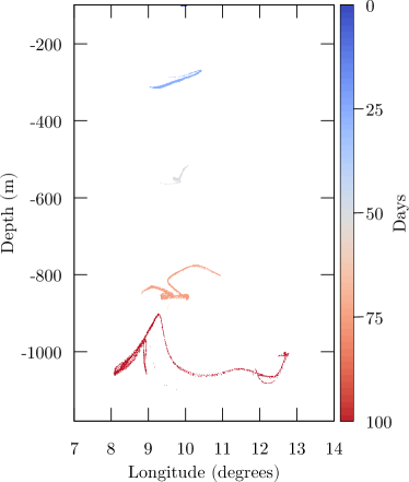
Figure 1: The positions of particles (projected onto a vertical plane) at different times in a realistic ROMS simulation Gutknecht et al. (2013) of the Benguela zone. The numerical experiment consisted of releasing $6000$ particles from initial conditions randomly chosen in a square with sides of $1/6^{\circ}$, centered at $10.0^{\circ}$ E $29.12^{\circ}$ S and $100\mathrm{m}$ depth. The particles’ trajectories $\mathbf{X}(t)$ were calculated from $\mathrm{d}\mathbf{X}/\mathrm{d}t=\mathbf{v}_{\mathrm{ROMS}}-W\hat{\mathbf{k}}$, where $\mathbf{v}_{\mathrm{ROMS}}$ is the velocity from the ROMS model, and $W=10\mathrm{m/day}$ corresponds to the sinking velocity Monroy et al. (2017), pointing in the vertical direction given by the unit vector $\hat{\mathbf{k}}$.

Preliminary numerical studies in a realistic oceanic setting showed that a homogeneous layer of particles (with neglecting the interaction between them) indeed evolves to complicated shapes by stretching and folding while it is sinking. As a motivation, Fig. 1 presents such a direct numerical simulation. It is clear that homogeneization or simplification is not reached on the time scale of the sinking process. The example of oceanic sedimentation thus emphasizes the practical importance of the investigation of non-asymptotic time scales in general, which, from a practical point of view, has received relatively little attention in the literature so far (an important exception is the paradigmatic problem of weather forecasting).

Beyond stretching and folding during the sinking process, an important additional ingredient for the emergence of observable inhomogeneities in the density of sedimented particles is the accumulation at the bottom of the domain. This is a time-integration of the density at a two-dimensional subset of the full three-dimensional space, and this results in the translation of the complicated shapes to actual inhomogeneities without any coarse-graining: the conservation of density no longer holds for such time-integrated projections.

In this paper, we shall describe in detail how inhomogeneities in the accumulated density emerge in incompressible flows on non-asymptotic time scales. We will derive the basic mechanisms analytically, and we will investigate the properties of these mechanisms in a simplified kinematic flow, in order to focus on the particle dynamics.

The main results we achieve are: i) we identify and quantify two geometrical mechanisms contributing to the creation of inhomogeneities in the density: the stretching due to the flow and the projection onto the constant depth where the particles accumulate; ii) we obtain an explicit expression for the density at an arbitrary position of the accumulation level in terms of the trajectories arriving to that particular position; and iii) in the context of a simplified kinematic flow we study the dependence on parameters that are generic to the problem: the settling velocity, the depth of the accumulation level, and the amplitude of the fluctuating flow.

The paper is organized as follows. In Section II we establish the setup for our analysis. In Section III we obtain the expression for the final density, and quantify the above-mentioned two effects leading to inhomogeneities. In Section IV we evaluate these results in the kinematic flow model. This flow is defined in two dimensions (one horizontal and one vertical), and it may show chaotic behavior. The role of the chaoticity of the flow will be explicitly addressed. In Section V we study the parameter dependence. Finally, in Section VI we summarize and comment on the results. A number of appendices contain the more technical aspects of our Paper.

II Formulation of the setup

II.1 Equations of motion

In this work we will consider the motion of particles that follow closely the velocity of the fluid in which they are dispersed, except for the addition of a constant vertical velocity arising from the particle weight. This description is adequate in a variety of circumstances. In particular it was shown by Monroy et al. Monroy et al. (2017) to be the adequate one to describe a wide range of biogenic particles sedimenting in ocean flows with turbulent intensity typical of the open ocean. We revise in the following the arguments leading to that conclusion.

The dynamics of spherical particles advected in fluids is described, in the small-particle limit, by the Maxey–Riley–Gatignol equation Maxey and Riley (1983); Haller and Sapsis (2008); Monroy et al. (2017). When writing it in a nondimensionalized form that uses the characteristic length $L$ and magnitude $U$ of the fluid velocity field as units of space and velocity, two relevant dimensionless parameters appear. The first one is the Stokes number:

$$\mathrm{St}=\frac{a^{2}U}{3\nu\beta L},$$ (1)

where $a$ is the radius of the particle, $\nu$ is the kinematic viscosity of the fluid, and $\beta=3\rho_{\mathrm{f}}/(2\rho_{\mathrm{p}}+\rho_{\mathrm{f}})$, with $\rho_{\mathrm{p}}$ and $\rho_{\mathrm{f}}$ being the densities of the particle and of the fluid, respectively. This number quantifies the importance of inertia with respect to viscous drag. The second dimensionless quantity is the Froude number, quantifying the importance of inertia with respect to gravity:

$$\mathrm{Fr}=\frac{U}{\sqrt{gL}},$$ (2)

where $g$ is the gravitational acceleration. In terms of these numbers, the dimensionless terminal settling velocity of a particle in still fluid is

$$W=(1-\beta)\frac{\mathrm{St}}{\mathrm{Fr^{2}}}\ .$$ (3)

In complex turbulent flows such as in the ocean, the values of $\mathrm{St}$ and $\mathrm{Fr}$ vary with scale. Monroy et al. Monroy et al. (2017) showed that for a relevant range of sizes and densities of biogenic particles, $\mathrm{St}$ is very small. For example, it takes valuesMonroy et al. (2017) in the range $10^{-7}\ldots 10^{-1}$ in wind-driven surface turbulence in the open ocean at the Kolmogorov scale ($\sim 0.3\ldots 2\mathrm{mm}$), whereJimenez (1997) typical turbulent velocities are in the range $0.5\ldots 3\mathrm{mm}/\mathrm{s}$. At larger scales, $\mathrm{St}$ is still smaller. For example, for mesoscale oceanic motions, $L_{\mathrm{h}}=100\mathrm{km}$ and $U_{\mathrm{h}}=0.1\mathrm{m/s}$ for horizontal motion, and $L_{\mathrm{v}}=100\mathrm{m}$ and $U_{\mathrm{v}}=10\mathrm{m/day}\approx 10^{-4}\mathrm{m/s}$ for vertical motion. This gives $\mathrm{St}\approx 10^{-6}$ for both horizontal and vertical motion. In any case, $\mathrm{St}$ is typically very small for the type of particles we are interested in. Under these circumstances a standard approachHaller and Sapsis (2008) can be used to approximate the equation of motion for the particle in the limit of vanishing $\mathrm{St}$ (see Appendix A, and Eq. (30) in particular), provided that the settling velocity $W$ is also small (Eq. (3)).

In our ocean situation, the Froude number ranges from $10^{-5}$ at the mesoscale to a maximum of $10^{-2}$ at the Kolmogorov scale. Thus, the combination $\mathrm{St}/\mathrm{Fr}^{2}$, appearing in the settling velocity $W$, Eq. (3), is within few orders of magnitude from $1$, and is typically larger than $1$. This means, first, that $W$ is always orders of magnitude larger than $\mathrm{St}$, $W\gg\mathrm{St}$, and, second, that $W$ is typically not a small quantity.

If $W\ll 1$ does not hold, the standard approachHaller and Sapsis (2008) for the small-$\mathrm{St}$ approximation is incorrect. In this case, what is appropriate is to take the limit defined by $\mathrm{St}\to 0$ and $\mathrm{Fr}\to 0$ with the value of $W\sim\mathrm{St}/\mathrm{Fr}^{2}$ remaining constant. Both in this new limit (see Appendix A) and in the standard approachHaller and Sapsis (2008) with $W\gg\mathrm{St}$, the leading order contribution in $\mathrm{St}$ to the equation of motion for the particle is a well-knownSiegel and Deuser (1997); Siegel, Fields, and Buesseler (2008); Qiu, Doglioli, and Carlotti (2014); Roullier et al. (2014); Monroy et al. (2017) approximation:

$$\dot{\mathbf{X}}=\mathbf{v}(\mathbf{X},t)\equiv\mathbf{v}_{\mathrm{fluid}}(\mathbf{X},t)-W\hat{\mathbf{k}}\ ,$$ (4)

where we have introduced the notation $\mathbf{v}$ for the “velocity field of the particle”. An important feature of the approximate Eq. (4) is the absence of any inertial term.

The description (4) would be applicable in other circumstances beyond the ones described above, but, of course, there would be situations — for example, coastal wave-breaking turbulence environments, industrial flows, or (other) cases in which $\mathrm{St}$ is not small enough — in which inertial terms will have central importance, with effects that have been studied in recent works Balkovsky, Falkovich, and Fouxon (2001); Bec (2003); Vilela et al. (2007); Cartwright et al. (2010); Guseva, Feudel, and Tél (2013); Guseva et al. (2016).

In our paper, we shall restrict our investigations to dynamics of the form of Eq. (4). Additionally, we shall assume $|v_{\mathrm{fluid},z}(\mathbf{X},t)|<W$ for the vertical component of the fluid velocity field, which ensures $v_{z}<0$ for the vertical component of the “particle velocity field” $\mathbf{v}$. This assumption excludes the presence of particle trajectories that would be trapped forever to the system, which simplifies the technical treatment of the problem and the interpretation of the phenomenology in that the accumulated density at the bottom of the domain is obtained by integrating over finite times. This assumption is reasonable in the above-discussed example of oceanic biogenic particles serving as our motivation Monroy et al. (2017).

II.2 Definitions

Let us consider a flow in a $d$-dimensional space in which we distinguish a ‘vertical’ direction, characterized by the ‘vertical’ coordinate $z$, and the remaining $(d-1)$-dimensional subspace, which we call ‘horizontal’, with the position vector $\mathbf{x}=(x,y,\ldots)=(x_{1},x_{2},\ldots,x_{d-1})$. We analyze the case $d=2$ in detail, with mentioning $d=3$ at some points due to its practical relevance, but all results can easily be generalized to higher dimensions, which can be useful when analyzing problems with phase spaces of higher dimensionality. The flow is defined by the velocity field $\mathbf{v}(\mathbf{X},t)$, $\mathbf{X}=(\mathbf{x},z)=(x,y,\ldots,z)=(x_{1},x_{2},\ldots,x_{d})$ being the position vector in the full space and $t$ being time. $v_{z}<0$ is assumed for all $\mathbf{X}$ and $t$.

We initialize noninertial particles at $t=t_{0}$ on a given level $z=z_{0}$ whose density within the so-defined horizontal subspace (a material line and surface for $d=2$ and $d=3$, respectively) is described by a “surface” density $\sigma$. We let the particles fall until all of them reach a depth $z=-a$ where they accumulate. We are interested in the resulting horizontal “surface” density $\sigma_{\parallel}$ of the particles measured within the accumulation level.

In our notation, a vertical line with a variable in the lower index, $\left.\right|_{\alpha}$, corresponds to keeping that particular variable, $\alpha$, constant, while a vertical line with the declaration of a value, $\left.\right|_{\beta=\beta_{0}}$, denotes evaluating the preceding expression at the indicated value, $\beta_{0}$. These two notations can also occur together. As an implicit rule in our notation, when taking derivatives with respect to a horizontal coordinate, all other horizontal coordinates are assumed to be kept constant.

III Relating the density to particle trajectories

The final density $\sigma_{\parallel}$ forming at any position of the accumulation level can be related to geometric properties of the flow observable along the trajectory of a particle that was initialized on the initial level $z_{0}$ at $t_{0}$ and that arrives at the given position. If we have more particles, the corresponding densities are to be added. In this Section we first explain that the relation can be given in terms of a special Jacobian, and analyze the formula from some practical aspects. Then we present (for simplicity, taking $d=2$ in the main text) an intuitive way of building up our formula, which lets us distinguish between the contribution of two simple effects: the stretching within the material line or material surface in which the particles are distributed, and the horizontal kinematic projection (i.e., a projection that takes the horizontal component of the velocity into account) of the density at the points of arrival at the accumulation level. Each of these two effects is well-defined even in setups in which the other is absent.

III.1 General results

Let the endpoint of a trajectory at time $t$ that was initialized at $\mathbf{x}_{0}$ be denoted by $\mathbf{f}(t;\mathbf{x}_{0})=(f_{x}(t;\mathbf{x}_{0}),f_{y}(t;\mathbf{x}_{0}),\ldots,f_{z}(t;\mathbf{x}_{0}))=(f_{1}(t;\mathbf{x}_{0}),f_{2}(t;\mathbf{x}_{0}),\ldots,f_{d}(t;\mathbf{x}_{0}))$. The horizontal density at the point where a particular trajectory crosses the accumulation plane $z=-a$ is proportional to the density at the initial position of the given trajectory:

$$\sigma_{\parallel}(t(f_{z}=-a,\mathbf{x}_{0}),\mathbf{x}_{0})=\sigma(t=t_{0},\mathbf{x}_{0})\mathcal{F}(t(f_{z}=-a,\mathbf{x}_{0}),\mathbf{x}_{0}),$$ (5)

where $\mathbf{x}_{0}$ is the $d-1$ dimensional initial position at $t=t_{0}$ of the particular trajectory within the initial level $z=z_{0}$, $\sigma(t=t_{0},\mathbf{x}_{0})$ is the initial “surface” density at $\mathbf{x}_{0}$, and $\sigma_{\parallel}(t,\mathbf{x}_{0})$ is the horizontal “surface” density at the endpoint, at some time $t$, of the trajectory that was initialized at $\mathbf{x}_{0}$. The time $t$ of arrival at the accumulation level is unique, since $v_{z}<0$ is assumed, see Section II. This time depends on the vertical position of the accumulation level, where $f_{z}=-a$, and also on which trajectory is chosen, which is defined by the initial position $\mathbf{x}_{0}$. (More generally, an arbitrary time $t$ can be regarded as a function of any final vertical position $f_{z}$ and of the initial position $\mathbf{x}_{0}$, $t=t(f_{z},\mathbf{x}_{0})$. The relation $t(f_{z},\mathbf{x}_{0})$ is single-valued because of the assumption $v_{z}<0$.) In case more than one trajectory arrives at the same position within the accumulation level, the corresponding densities are summed up.

The total factor, $\mathcal{F}(t(f_{z}=-a,\mathbf{x}_{0}),\mathbf{x}_{0})$, that multiplies the original density at the starting point of the given trajectory, is the reciprocal of the determinant of a Jacobian:

$$\mathcal{F}(t(f_{z}=-a,\mathbf{x}_{0}),\mathbf{x}_{0})=\det\left(J(t(f_{z}=-a,\mathbf{x}_{0}),\mathbf{x}_{0})\right)^{-1},$$ (6)

where $J$ is a $(d-1)\times(d-1)$ Jacobian:

$$J_{ij}(t(f_{z},\mathbf{x}_{0}),\mathbf{x}_{0})=\left.\frac{\partial f_{j}(t(f_{z},\mathbf{x}_{0}),\mathbf{x}_{0})}{\partial x_{0i}}\right|_{f_{z}}$$ (7)

for $i,j\in\{1,\ldots,d-1\}$. This Jacobian is not a usual one in two aspects. First, it is not a full-dimensional Jacobian, but it is restricted to the horizontal coordinates. In particular, for flows with $d=2$, it is a scalar. Second, the derivatives with respect to the coordinates of $\mathbf{x}_{0}$ are taken at a constant value of the vertical coordinate $f_{z}$, and not at a constant time. For this reason, the direct numerical evaluation of Eq. (7) for a given trajectory is not straightforward. Nevertheless, Eqs. (6)-(7) are intuitive in the sense that they give the ratio between the final and the initial values of the “area” of an infinitesimal “surface” element neighboring the given trajectory within the material “surface” of particles. For a more rigorous derivation, see Appendix B. Note that the determinant of a full-dimensional Jacobian taken at a constant time is always one for volume-preserving flows. In our setup, the reduced dimensionality and the non-instantaneous accumulation process lead to changes in the density, and thus the formation of inhomogeneities becomes possible.

We show in Appendix C that the derivatives taken at a constant $f_{z}$ in the Jacobian (7) can be replaced by derivatives taken at a constant time $t$ in the following way:

$$\left.\frac{\partial f_{i}(t(f_{z},\mathbf{x}_{0}),\mathbf{x}_{0})}{\partial x_{0j}}\right|_{f_{z}}=\left.\frac{\partial f_{i}(t,\mathbf{x}_{0})}{\partial x_{0j}}\right|_{t}-\frac{v_{i}(t,\mathbf{f}(t;\mathbf{x}_{0}))}{v_{z}(t,\mathbf{f}(t;\mathbf{x}_{0}))}\left.\frac{\partial f_{z}(t,\mathbf{x}_{0})}{\partial x_{0j}}\right|_{t},$$ (8)

for $i,j\in\{1,\ldots,d-1\}$. The difference between taking derivatives at constant $f_{z}$ and constant $t$ stems from the fact that different trajectories in the material “surface” reach a given level $f_{z}$ at different times $t$. From a practical point of view, Eq. (8) can easily be evaluated numerically.

Transforming the right-hand side of Eq. (6) in an alternative way, we learn that it can be obtained from an integral along the given trajectory (as derived in Appendix D):

$$\mathcal{F}(t(f_{z}=-a,\mathbf{x}_{0}),\mathbf{x}_{0})=\exp\left(-\int_{z_{0}}^{-a}\left.\sum_{i=1}^{d-1}\frac{\partial}{\partial f_{i}}\left(\frac{\hat{v}_{i}(f_{z},\mathbf{f}_{\parallel})}{\hat{v}_{z}(f_{z},\mathbf{f}_{\parallel})}\right)\right|_{f_{z},\mathbf{f}_{\parallel}=\mathbf{f}_{\parallel}(f_{z},\mathbf{x}_{0})}\mathrm{d}f_{z}\right),$$ (9)

where $\mathbf{f}_{\parallel}=(f_{1},\ldots,f_{d-1})$ denotes the horizontal coordinates of the trajectory, and $\hat{v}_{i}(f_{z},\mathbf{f}_{\parallel})=v_{i}(t(f_{z},\mathbf{x}_{0}(f_{z},\mathbf{f}_{\parallel})),\mathbf{f}(t(f_{z},\mathbf{x}_{0}(f_{z},\mathbf{f}_{\parallel})),\mathbf{x}_{0}(f_{z},\mathbf{f}_{\parallel})))$ for $i\in\{1,\ldots,d\}$, i.e., $\hat{\mathbf{v}}(f_{z},\mathbf{f}_{\parallel})$ is the velocity as regarded as a function of the endpoints of the trajectories (instead of the time and the “bare” geometrical coordinates of the domain of the fluid flow). When keeping $f_{z}$ constant, the derivatives taken with respect to the coordinates $f_{i}$, with $i\in\{1,\ldots,d-1\}$, correspond to varying the selected trajectory and also the time $t$, so that these derivatives are not the instantaneous geometrical derivatives of the velocity field (see Appendix D for a more detailed explanation). By replacing the derivatives taken at a constant $f_{z}$ with those taken at a constant $t$, we can further transform our formula such that it can be directly evaluated numerically, see Appendix E.

One important aspect of the results presented in this Section is that the final density at a given point can be obtained in terms of the initial density at one point (or, at least, a countable number of them) and of the particle trajectory (or trajectories) linking the points: these are all local properties, and no spatially extended information (within the material “surface”) is needed to determine the final density at the given point. In the next subsection we rewrite Eqs. (6)-(8) in alternative ways which highlight the contributions from two different and physically intuitive processes.

III.2 Stretching and projection

In this Section we obtain Eq. (6)-(8) via two physically intuitive steps which correspond to two individual effects that modify the original density. For simplicity, we restrict ourselves to $d=2$. In order to be able to precisely formulate our considerations, we use a parametric notation for the material line in this Section.

Let $\mathbf{f}(t=t_{0};u)$ describe a line segment of initial conditions at time $t=t_{0}$ (a material line of particles) embedded in 2 dimensions, parameterized by the arc length $u$, and let $\sigma(t=t_{0};u)$ be the initial density along the line segment at $u$. Note that the initial line segment need not be horizontal: the results of this Section apply for a 1-dimensional initial subset of arbitrary shape, which extends the validity of these considerations to more general setups.

Let us denote the image of the initial line segment at time $t$ by $\mathbf{f}(t;u)$. The density $\sigma(t;u)$ along this image at $t$ in a point whose initial position was characterized by $u$ is given by

$$\sigma(t;u)=\sigma(t=t_{0};u)\mathcal{S}(t;u),$$ (10)

where

$$\mathcal{S}(t;u)=\left|\frac{\mathrm{d}\mathbf{f}(t;u)}{\mathrm{d}u}\right|^{-1}.$$ (11)

This simply follows from imposing the conservation of mass (i.e., continuity) within the material line of the particles. Note that the density (due to the incompressibility of the fluid) is conserved only in the full space, but not along subsets with lower dimensionality. For a precise derivation based on the full-dimensional density, see Appendix H. The factor $\mathcal{S}(t;u)$, multiplying the original density, describes the stretching along the material line up to time $t$ experienced near a particle initialized at position $u$.

We can obtain the horizontal density $\sigma_{\parallel}(t;u)$ by projecting the instantaneous density $\sigma(t;u)$, which is measured along the material line, to the horizontal direction taking into account the kinematics of the problem. In particular, we need to take into account the instantaneous orientation of the material line at the position characterized by $u$, and also the velocity at the same position:

$$\sigma_{\parallel}(t;u)=\sigma(t;u)\mathcal{P}(t;u),$$ (12)

where, according to simple geometry relating the pre- and the post-projection length of an infinitesimal segment of the material line around the position characterized by $u$,

$$\mathcal{P}(t;u)=\left|\frac{\mathrm{d}f_{x}(t;u)}{\mathrm{d}s}-\frac{\mathrm{d}f_{z}(t;u)}{\mathrm{d}s}\frac{v_{x}(\mathbf{f}(t;u),t)}{v_{z}(\mathbf{f}(t;u),t)}\right|^{-1}.$$ (13)

Here $s$ is the arc length along the image of the line segment at $t$, and $u$ can be regarded as a function of $s$. The first term holds alone when there is no horizontal velocity at the given time instant at the position of the given particle, and the second term originates from an additional change in the length, which is due to the presence of horizontal motion. It is worth emphasizing that the presence of the second term is due to projecting the material line to a given depth, instead of taking the projection at a given time, in agreement with Eq. (7). For a more detailed explanation of the formula, see Appendix I. This relation is valid for any $t$ and $u$, so that it also applies to the time instant when a given particle arrives at the accumulation level.

In total, there are two independent effects modifying the initial density $\sigma(t=t_{0};u)$: the stretching and the projection, and both of them appear as a factor multiplying $\sigma(t=t_{0};u)$:

$$\sigma_{\parallel}(t;u)=\sigma(t=t_{0};u)\mathcal{F}(t;u)=\sigma(t=t_{0};u)\mathcal{S}(t;u)\mathcal{P}(t;u),$$ (14)

where $\mathcal{F}(t;u)$ is the total factor (the same as in (6), for $d=2$), and $\mathcal{S}(t;u)$ and $\mathcal{P}(t;u)$ correspond to the stretching and the projection as defined by Eqs. (11) and Eq. (13), respectively.

We can simplify the total factor to obtain (6) with (8) as follows. Applying the chain rule for the partial derivatives in (13) yields

$$\mathcal{P}(t;u)=\left|\frac{\mathrm{d}\mathbf{f}(t;u)}{\mathrm{d}u}\right|\left|\frac{\mathrm{d}f_{x}(t;u)}{\mathrm{d}u}-\frac{\mathrm{d}f_{z}(t;u)}{\mathrm{d}u}\frac{v_{x}(\mathbf{f}(t;u),t)}{v_{z}(\mathbf{f}(t;u),t)}\right|^{-1},$$ (15)

where

$$\left|\frac{\mathrm{d}u}{\mathrm{d}s}\right|=\left|\frac{\mathrm{d}\mathbf{f}(t;u)}{\mathrm{d}u}\right|^{-1}$$ (16)

has been used (see Eq. (75) and the preceding discussion in Appendix H). Note that, according to (11),

$$\left|\frac{\mathrm{d}\mathbf{f}(t;u)}{\mathrm{d}u}\right|=\mathcal{S}(t;u)^{-1},$$ (17)

the substitution of which into (15) cancels out $\mathcal{S}(t;u)$ in (14):

$$\mathcal{F}(t;u)=\left|\frac{\mathrm{d}f_{x}(t;u)}{\mathrm{d}u}-\frac{\mathrm{d}f_{z}(t;u)}{\mathrm{d}u}\frac{v_{x}(\mathbf{f}(t;u),t)}{v_{z}(\mathbf{f}(t;u),t)}\right|^{-1},$$ (18)

which is equivalent to (6)-(8) for $d=2$.

The first term in Eq. (18),

$$\delta_{x}(t;u)=\frac{\mathrm{d}f_{x}(t;u)}{\mathrm{d}u},$$ (19)

is the parametric derivative, with respect to the position along the initial line segment, of the horizontal component of the current position vector, while the second term,

$$\tilde{\delta}_{z}(t;u)=-\delta_{z}(t;u)\frac{v_{x}(\mathbf{f}(t;u),t)}{v_{z}(\mathbf{f}(t;u),t)}=-\frac{\mathrm{d}f_{z}(t;u)}{\mathrm{d}u}\frac{v_{x}(\mathbf{f}(t;u),t)}{v_{z}(\mathbf{f}(t;u),t)},$$ (20)

is its vertical counterpart, but it is weighted by the ratio of the two velocity components. As in Eq. (13), the former one is due to a “static” change in length (i.e., not influenced by any horizontal motion), and the latter one is the “correction” when horizontal motion is present. The possibility of simplifying Eq. (14) (with Eqs. (11) and Eq. (13)) to Eq. (18) is not a surprise: it is only the ratio between the final and the initial length of an infinitesimal line segment that is relevant, which we have already learnt in Section III.1.

Results for $d=3$ corresponding to those of this Section discussed so far are given in Appendix J, and formulae for $d>3$ can be constructed similarly.

For $d=2$, we can summarize our final expression as

$$\sigma_{\parallel}(t;u) =\sigma(t=t_{0};u)\mathcal{F}(t;u)$$

$$=\sigma(t=t_{0};u)\mathcal{S}(t;u)\mathcal{P}(t;u)$$

$$=\sigma(t=t_{0};u)\left|\delta_{x}(t;u)+\tilde{\delta}_{z}(t;u)\right|^{-1},$$ (21)

with the particular quantities collected in Table 1. Note that a special situation may occur for those trajectories for which $|\delta_{x}+\tilde{\delta}_{z}|=0$ at the accumulation level. In this case the final horizontal density is unbounded. The corresponding positions within the accumulation level characterize the so-called (density) caustics Wilkinson and Mehlig (2005), and they refer to the maximum levels of inhomogeneity in the accumulated density, so that their identification and dependence on parameters is of great relevance in our work. Of course, the integral of the density (with respect to the final horizontal coordinate $x$) over such caustics remains finite. In particular, the generic form of a density caustic originating from a standard parabolic fold with its vertex located at $x_{\mathrm{c}}$ is $\sim 1/\sqrt{x-x_{\mathrm{c}}}$.

Notation	Name	Defining formula
$\mathcal{F}$	Total factor	(14)
$\mathcal{S}$	Stretching factor	(11)
$\mathcal{P}$	Projection factor	(13)
$\delta_{x}$	Parametric derivative of the horizontal position	(19)
$\delta_{z}$	Parametric derivative of the vertical position	(20)
$\tilde{\delta}_{z}$	Weighted parametric derivative of the vertical position	(20)

Table 1: The main quantities relevant for changes in the density.

We can give a more intuitive condition for the positions of the caustics. We first recognize a simplification of (13), which is useful in general, too, and reads as

$$\mathcal{P}(t;u)=\left|\frac{v_{z}(\mathbf{f}(t;u),t)}{\mathbf{n}(t;u)\cdot\mathbf{v}(\mathbf{f}(t;u),t)}\right|,$$ (22)

where $\mathbf{n}(t;u)$ is the normal vector of the line $\mathbf{f}$ at time $t$ at a position that is characterized by $u$. Eq. (22) is true, since $\mathbf{n}$ is obtained by rotating the tangent vector $\mathrm{d}\mathbf{f}/\mathrm{d}s$ of the line by $\pi/2$:

$$\mathbf{n}(t;u)=\left(-\frac{\mathrm{d}f_{z}(t;u)}{\mathrm{d}s},\frac{\mathrm{d}f_{x}(t;u)}{\mathrm{d}s}\right).$$ (23)

A remarkable property of (22) is that it remains valid for $d=3$, see Appendix K for the derivation.

The presence of caustics actually originates from the projection factor $\mathcal{P}$ alone, and Eq. (22) gives a particularly intuitive interpretation by identifying the positions of the caustics as

$$\mathbf{n}(t;u)\cdot\mathbf{v}(\mathbf{f}(t;u),t)=0.$$ (24)

That is, caustics appear in the accumulation plane wherever the local normal vector of the line is perpendicular to the local velocity, or, equivalently, where the local tangent of the line coincides with the direction of the local velocity.

IV Numerical examples

In this Section we present the basic phenomenology of our setup via numerical examples in a 2D model flow.

IV.1 Model flow

The equation of motion for the particles, Eq. (4), relies on a fluid flow $\mathbf{v}_{\mathrm{fluid}}(\mathbf{X},t)$. For clarity, we choose this velocity field to have zero mean integrated over space. Note, however, that as long as the spatial distribution of the particles is inhomogeneous, the vertical velocity averaged over all particles will be different from $-W$ due to the inhomogeneities of the velocity field Drótos and Tél (2011).

In order to present relevant phenomena in a clear way, we use a $d=2$ model flow $\mathbf{v}_{\mathrm{fluid}}(\mathbf{X},t)$ for our numerical examples: we choose a modified version of the paradigmatic double-shear flow Pierrehumbert (1994). In its classical version, it is a periodic velocity field consisting of a horizontal shear during the first half of the temporal period and of a vertical shear during the other half. We modify this in two aspects: First, we smooth the discontinuous transition between the two orientations by introducing a hyperbolic-tangent-type transition Vilela et al. (2007). Second, we rotate the shear directions by 45 degrees, to break the coincidence of the two instantaneous velocity directions with the horizontal and vertical axes, which in our sedimentation setup have a very specific role. The resulting velocity field is written as:

$$v_{\mathrm{fluid},x}(\mathbf{X},t) =\frac{1}{\sqrt{2}}(v_{\mathrm{fluid},\xi}(\mathbf{X},t)-v_{\mathrm{fluid},\eta}(\mathbf{X},t)),$$ (25)

$$v_{\mathrm{fluid},z}(\mathbf{X},t) =\frac{1}{\sqrt{2}}(v_{\mathrm{fluid},\xi}(\mathbf{X},t)+v_{\mathrm{fluid},\eta}(\mathbf{X},t)),$$ (26)

where

$$v_{\mathrm{fluid},\xi}(\mathbf{X},t) =A(1+\tanh[\gamma\sin(2\pi t)])\sin[\sqrt{2}\pi(z-x)],$$ (27)

$$v_{\mathrm{fluid},\eta}(\mathbf{X},t) =A(1-\tanh[\gamma\sin(2\pi t)])\sin[\sqrt{2}\pi(z+x)].$$ (28)

$\gamma=20/\pi$ controls the temporal sharpness of the shear-direction switching, it is fixed throughout the paper (as well as the temporal period of the fluid, which is set to $1$). $A$ is half of the amplitude of each elementary velocity component (in what follows: the ‘amplitude’). By increasing $A$ we increase the strength of the flow and, as a consequence, also its chaoticity, i.e., the (largest positive) Lyapunov exponent, which is associated to the separation with time of fluid particle trajectories. Note that the velocity field (26)-(28) is also periodic in space, with a period of $\sqrt{2}$ in both $x$ and $z$. For the trajectories, at variance with other implementations of flows related to the double shear, we do not impose any periodic boundary conditions, so that the particles’ positions evolve in the unbounded directions $x$ and $z$.

If we regard the accumulation level as the bottom of the domain of a realistic fluid flow, the velocity field $\mathbf{v}_{\mathrm{fluid}}(\mathbf{X},t)$ would have to fulfill a no-flux or even a no-slip boundary condition at $z=-a$, which is not satisfied by (26)-(28).

As for the no-flux boundary condition, we do not expect to introduce any qualitative difference compared to the results obtained in our example flow, since in all our theoretical formulae the relevant quantity at the accumulation level appears to be not the fluid velocity $\mathbf{v}_{\mathrm{fluid}}$, but the particle velocity $\mathbf{v}$, which would not have a vanishing vertical component. Indeed, we carried out our main analyses in a different flow, namely a spatially periodic sheared vortex flow with temporal modulation Feudel et al. (2005); Lindner and Donner (2017), with accumulation levels fulfilling the no-flux boundary condition, and obtained the very same qualitative results.

In principle, a viscous boundary layer with a so-slip boundary condition, or any kind of a separate flow regime at the bottom of the fluid with different characteristics compared to the bulk (e.g. length and time scales, magnitude of the velocity), cannot be excluded to leave an important, specific imprint on the qualitative properties of the accumulated particle density. However, with our assumptions and parameters, as well as in oceanic settings, the time that is spent by a particle in a given layer is mainly determined by the settling velocity $W$, independent of the flow, hence the effects of any boundary layer or separate flow regime are expected to be negligible if the boundary layer is thin compared to the bulk of the fluid (like in the ocean).

Beyond all of the above, in experimental set-ups such as in sediment traps, the accumulation points are not at the bottom of the sea, but at some intermediate depth at which no boundary conditions apply at all.

IV.2 Illustrative results

We now present typical examples for the final density within the accumulation level, and show how its form emerges from the reshaping of the material line, which gives rise to the different density-modifying contributions that have been introduced in Section III. We always initialize, at $t_{0}=0$, $10\,000$ particles at $z_{0}=0$ uniformly in a line segment $x\in[0,1]$. (Note that any initial length of the order of unity would suffice for our examples.) We follow the particles’ trajectories in the double-shear flow Eq. (26), and compute the relevant quantities numerically (see Table 1). When more than one branch of the material line arrives at the same position (as a result of folding), we additionally calculate the sum $\sum\mathcal{F}$ of the total factors $\mathcal{F}$ corresponding to the individual branches. Furthermore, we compare $\sum\mathcal{F}$ to a normalized histogram $h$ calculated directly from the arrival positions of the individual particles.

We start with a parameter setting that does not produce noticeable chaos, but leads to regular motion: the portrait of the corresponding stroboscopic map consists of slightly undulating quasi-vertical lines. However, the net horizontal displacement of a trajectory after vertically traversing one spatial period of the flow is not zero generally, it is just very small.

(a)

(b)

(c)

Figure 2: The positions of the particles of the initially horizontal material line of unit length, at the indicated time instants. Dashed lines mark the accumulation levels taken for Figs. 3, 4, and 5. $A=0.06$, $W=0.6$.

Snaphots from the time evolution of the line of particles are shown in Fig. 2. At the beginning, both horizontal and relative vertical displacements of neighboring particles remain small, and the line becomes slightly undulated (Fig. 2a). Later on, relative vertical displacements become much larger, see Fig. 2b. When they become large enough, it can happen that certain, more slowly falling, parts of the line are folded above the faster parts, as can be observed in Fig. 2c. Such folds, together with the nearly vertical velocity vector, result in caustics after accumulation.

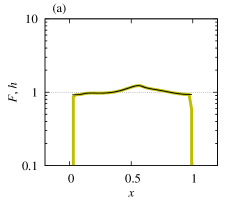
(a)

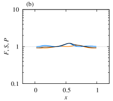
(b)

(c)

Figure 3: (a) The total factor $\mathcal{F}$, at the accumulation level $a=2.7$ (marked by a horizontal dashed line in Fig. 2a), computed along the individual trajectories according to (18) (in black), and the histogram $h$ (with bin size $0.02$) obtained from the positions of the trajectories on the accumulation level (in dark yellow), both as a function of the position along the accumulation level. (b) The total factor $\mathcal{F}$ (black) compared to the stretching factor $\mathcal{S}$ (orange) and to the projection factor $\mathcal{P}$ (blue). (c) The reciprocal of the total factor $\mathcal{F}$ (black) compared to the parametric derivative of the horizontal position $\delta_{x}$ (green), to the parametric derivative of the vertical position $\delta_{z}$ (thin magenta) and to the weighted parametric derivative of the vertical position $\tilde{\delta}_{z}$ (thick magenta). See Table 1 to locate the corresponding formulae. $A=0.06$, $W=0.6$.

Figure 3 considers the parameter setting of Fig. 2, and shows the quantities of Table 1 for an accumulation level placed at $z=-a=-2.7$ (marked also in Fig. 2a). We can see in Fig. 3a that the total factor $\mathcal{F}$ computed along the individual trajectories according to (18) gives practically perfectly the same result as directly calculating the histogram $h$ from the positions of the trajectories on the accumulation level. The total factor does not take a constant value of $1$, so that the density develops inhomogeneities, but only weak ones, which depend smoothly on the position along the accumulation level.

In Fig. 3b, we can observe that the smooth “undulation” of the total factor $\mathcal{F}$ originates from rather generic “undulations” of the stretching factor $\mathcal{S}$ and the projection factor $\mathcal{P}$, the deviation of which from $1$ is of similar magnitude as that of $\mathcal{F}$. A little bit more interesting is Fig. 3c, which analyzes the contributions from the different terms in the reciprocal of the total factor $\mathcal{F}$. Due to the weak horizontal displacements, a unit change along the initial, horizontally oriented material line segment approximately results in a unit change along the accumulation depth as well. As a consequence, the value of the parametric derivative $\delta_{x}$ is near to $1$. The parametric derivative $\delta_{z}$, however, deviates more from its initial value of $0$, which indicates that relative vertical displacements are stronger. Nevertheless, from the point of view of the density, weighting this parametric derivative by $v_{x}/v_{z}$ to obtain $\tilde{\delta}_{z}$ keeps the effect of stronger relative vertical displacements small: the amplitude $A$ of the fluctuating part of the velocity field, contributing alone to $v_{x}$, is much smaller than $W$, which dominates in $v_{z}$.

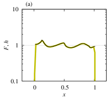
(a)

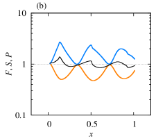
(b)

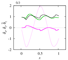
(c)

Figure 4: Same as Fig. 3 for a deeper accumulation depth, $a=16.2$ (marked by a horizontal dashed line in Fig. 2b).

If we let the line fall more and prescribe $z=-a=-16.2$ (seen in Fig. 2b), the “undulation” of the total factor $\mathcal{F}$, of course, becomes stronger, see Fig. 4a. It may be surprising that stretching and projection both have even much stronger effect, shown in Fig. 4b, but they are approximately anticorrelated, so that they more or less cancel out each other (note that $\mathcal{S}$ and $\mathcal{P}$ are multiplied in (14), and are shown on a logarithmic scale in 4b). Qualitatively, this can be understood as a result of the relative vertical displacements being much larger than the horizontal ones, which is clearly observable in Fig. 2b: both the stretching and the tilting of the line result mainly from the vertical deformation, and, when different parts of the line are accumulated on the same level, with a nearly vertical velocity ($v_{x}/v_{z}$ is still small), this deformation is practically removed, resulting in an approximately homogeneous horizontal line after projection.

An open question is why horizontal displacements are much smaller than vertical ones. Note that the amplitude of the shear flow is the same in the vertical and the horizontal directions. The phenomenon is certainly due to the symmetry breaking introduced by the settling term in the velocity (4). We shall return to the possible importance of this phenomenon in Section V.3.

Note in Fig. 4b that stretching almost always dilutes the original density, while projection almost always densifies it. While this already follows from the geometry of the line in Fig. 2b, we can easily provide with a more general explanation: On the one hand, anyhow we initialize our material line segment, it will gradually align with the stretching direction (as opposed to shrinking). As for the projection, on the other hand, the simple horizontal projection of an (in our case, curved) line is always shorter than the original line. This can only be altered by a strong horizontal velocity component, but $v_{x}/v_{z}$ is small here.

Figure 4c confirms our visual observation (in Fig. 2b) of the strong vertical and relatively weak horizontal deformation, and emphasizes the importance of the smallness of $v_{x}/v_{z}$ in avoiding strong modifications of the density.

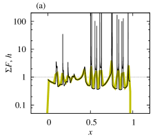
(a)

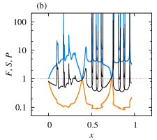
(b)

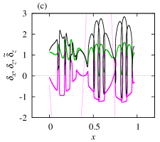
(c)

Figure 5: Same as Fig. 3 for $a=97.2$ (marked by a horizontal dashed line in Fig. 2c), and panel (a) showing the total factor $\mathcal{F}$ summed over the different branches of the material line segment.

In Fig. 5, accumulation is prescribed at an even deeper depth, $z=-a=-97.2$ (seen in Fig. 2c). As Fig. 2c shows, the line segment has undergone foldings by the time it reaches this accumulation level. At the folding points (note that they occur in pairs), where the tangent of the line coincides with the local velocity (see Eq. (24)), caustics appear: the projection factor $\mathcal{P}$ tends to infinity (blue line in Fig. 5b), and this is carried over also to the total factor $\mathcal{F}$ (black line in Fig. 5b). To obtain the total density forming along the accumulation level, the total factors $\mathcal{F}$ corresponding to each of the branches of the material line have to be summed up, see Fig. 5a. Fig. 5a also shows that our histogram $h$ is not able to resolve the caustics and fine structures.

The novelty in Fig. 5c is that even the weighted parametric derivative $\tilde{\delta}_{z}$ grows to considerable magnitudes, this is how it becomes possible that the sum $\delta_{x}+\tilde{\delta}_{z}$ crosses zero, where the caustics are found (see Eq. (21)). The unweighted parametric derivative $\delta_{z}$ is so large that it typically does not fit to the scale of the plot, which concentrates on the other quantities. Note also that $v_{x}$ changes sign near the caustics, which is not surprising: this is how folds can appear.

(a)

(b)

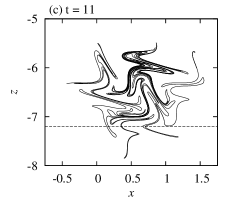
(c)

Figure 6: Same as Fig. 2 for $A=0.25$. The dashed lines in panels (a) and (c) mark the accumulation levels taken for Figs. 7 and 8.

Now we change our parameter setting to obtain a completely chaotic case, when the phase portrait shows homogeneous mixing. The time evolution of the geometry of the line of particles is shown in Fig. 6. Strong stretching occurs at the very beginning, which is accompanied soon by several folds (Fig. 6a). This is the situation that resembles the most to our motivating example in Fig. 1. Later on, rather complicated structures develop (Fig. 6b). Finally, the line follows finer and finer structures of the typical fractal filamentation of chaos (Fig. 6c). Unlike in Fig. 2, anisotropy in the relative displacement of neighboring particles is not obvious.

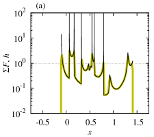
(a)

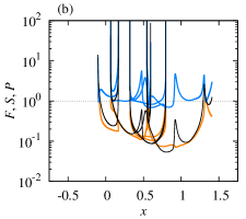
(b)

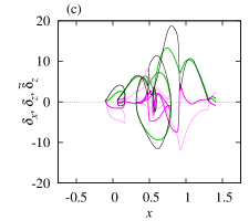
(c)

Figure 7: Same as Fig. 5 for $A=0.25$ and accumulation level $a=1.8$ (shown as a horizontal line in 6a).

For an accumulation level that is reached during the early stages of the development of the structures (see Fig. 6a), the summed total factor $\sum\mathcal{F}$, as well as the histogram $h$, exhibits considerable inhomogeneities, see Fig. 7a. (In this case, they are only the peaks of the caustics that are not resolved by $h$.) Therefore, we can say that chaos first inhomogeneizes the initially uniform distribution.

In Fig. 7b, we can observe that stretching dilutes, and projection densifies, in accordance with our general argumentation that we gave when discussing Fig. 4b.

In Fig. 7c, we can see that $\delta_{x}$ and $\delta_{z}$ have similar magnitude, lacking the anisotropy observed in Figs. 3-5. Furthermore, $\tilde{\delta}_{z}$ is not much smaller than $\delta_{z}$, due to the relatively strong amplitude $A$ of the flow compared to $W$.

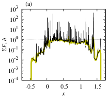
(a)

(b)

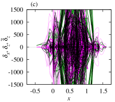
(c)

Figure 8: Same as Fig. 7 for $A=0.25$ and $a=7.2$ (shown as a horizontal line in 6c).

For an accumulation level placed at a depth where chaotic filamentation is rather developed (see Fig. 6c), the summed total factor $\sum\mathcal{F}$, shown in Fig. 8a, is composed of extremely many contributions from individual branches, and thus exhibits extremely many corresponding caustics. However, apart from the caustics and some fine-scale structures, the resulting shape is quite simple: it is a single bump. The histogram $h$, not being able, of course, to resolve the caustics, only “detects” this bump. This coarse-grained structure is resembling somewhat to the Gaussian that is expected to appear for asymptotically long times, and clearly indicates that chaos now homogeneizes earlier inhomogeneities (cf. Fig. 7), unless the density is investigated on a fine scale. Due to conservation of mass and the not very enhanced horizontal extension, the bulk of the bump is close to $1$ in Fig. 8a.

This is not so, however, before summing up the contributions from the different branches, see the black line, $\mathcal{F}$, in Fig. 8b. It is clear that stretching (represented by $\mathcal{S}$, orange line), which dilutes, “wins” as opposed to projection (represented by $\mathcal{P}$, blue line), which densifies. Chaos naturally involves very strong stretching. Projection, however, originates from local geometric properties: it is determined solely by the local orientation of the material line and the local velocity of the fluid where and when a particle of the line arrives at the accumulation depth. The local orientation of the line is, after strong enough mixing, practically random (with a possibly nonuniform distribution, determined by the flow). After reaching this randomness, the projection factor $\mathcal{P}$ will not grow any more, i.e., its magnitude saturates. At the same time, stretching can always grow. Note, however, that the projection factor $\mathcal{P}$ should also increase at the beginning.

In this last, chaotic case, the parametric derivatives of the horizontal and vertical positions behave in a completely irregular way, see Fig. 8c. The only conclusion that we can draw from Fig. 8c, based on some breaks in some lines, is that the resolution of the filamentation is reaching its limit with the current number of the particles.

V Systematic study of parameter dependence

It is an interesting question how inhomogeneities and the underlying effects, as presented in the previous Section, respond to changes in the parameters. For characterizing the basic properties of the quantities analyzed in Section IV.2, we evaluate their average and standard deviation along the accumulation level. The former gives the net effect (dilution or densification), while the latter characterizes the strength of inhomogeneities. We emphasize that evaluation along the accumulation level means that we evaluate the statistics with respect to horizontal length, but we do not sum up over possible different branches of the material line that are present at the same point within the accumulation level (except for the summed total factor $\sum\mathcal{F}$ and the normalized histogram $h$, the definition of which implies summation). In particular, the average of a quantity $\phi$, where $\phi$ is either $\mathcal{S}$, $\mathcal{P}$, $\mathcal{F}$, $\delta_{x}$, $\delta_{z}$ or $\tilde{\delta}_{z}$, is obtained as

$$\langle\phi\rangle=\sum_{i=1}^{n}\frac{1}{x_{i}-x_{i-1}}\int_{x_{i-1}}^{x_{i}}\phi\,\mathrm{d}x,$$ (29)

where $x$ is the horizontal coordinate along the accumulation level, $x_{1}$ and $x_{n}$ are the positions where the beginning and the endpoint of the material line reach the accumulation level, respectively, $x_{i}$ for $i\in\{2,\ldots,n-1\}$ are the positions of the caustics where the line undergoes a fold (note that $x_{i+1}<x_{i}$ if $x_{i}>x_{i-1}$ and vice versa, which implies that $n$, and also the number of the caustics, $n-2$, are even). The formula for the standard deviation is similar. Beyond averages and standard deviations, we shall also consider the number of the caustics.

We mention here that the standard deviation is not well-defined if caustics are present. Since caustics, as mentioned, are $1/\sqrt{x}$-type singularities in the density, the integral over their square, $1/x$, does not remain finite. Indeed, we numerically found that the standard deviation calculated from a normalized histogram $h$ grows approximately as $-\log\,\Delta x$ with the bin size $\Delta x$ of the histogram whenever the number of the caustics is greater than zero (should it be $2$ or several thousands), which is a characteristic of numerical integrals over $1/x$. Therefore, for such parameter values, we plot the standard deviation of the normalized histogram $h$, separately for a smaller and for a larger bin size, and do not show the numerically obtained standard deviation for $\sum\mathcal{F}$, $\mathcal{F}$ or $\mathcal{P}$. When calculating $h$ for different parameter values, we keep the number $N$ of the bins constant (instead of the bin size), and indicate $N$ in the lower index of $h$ as $h_{N}$.

We concentrate on the dependence on the following parameters: the settling velocity $W$, the accumulation depth $a$, and the amplitude of the fluctuating part of the velocity field, which corresponds to $A$ in Eq. (28). An important combination of these quantities is $\tau=a/W$, which is roughly proportional to the time needed for the material line to reach the accumulation level. The difference of $\tau$ from the actual settling time, when averaged over the particles, is due to the inhomogeneous spatial distribution of the particles, as explained in Section IV.1. Note, furthermore, that different parts of the material line reach the accumulation level at different times. This results in a smearout of the settling time along the line, which is also reflected in the properties that we investigate. As the vertical extension of the material line grows in time, or with increasing depth, the importance of this phenomenon also increases. At the beginning, the spread of the settling time is smaller than the characteristic time scale of the flow (i.e., unity), but later on it grows above this characteristic time. In spite of all this, the time $\tau$ gives a good guidance for the interpretation of what can be observed.

V.1 Dependence on the settling velocity $W$

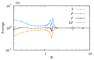
(a)

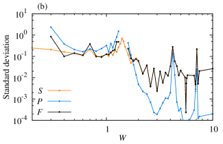
(b)

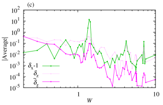
(c)

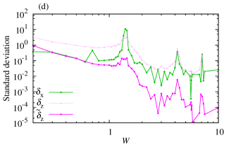
(d)

Figure 9: (a) The average and (b) the standard deviation, as a function of the settling velocity $W$, of the stretching factor $\mathcal{S}$, of the projection factor $\mathcal{P}$, and of the total factor $\mathcal{F}$, the latter also summed up over the different branches of the line in panel (a) (for the chosen values of $\tau$ and $A$, the result mostly coincides with the non-summed-up factor). (c)-(d) The same for the parametric derivative of the horizontal position $\delta_{x}$ (minus $1$ for comparability), the parametric derivative of the vertical position $\delta_{z}$, and the weighted parametric derivative of the vertical position $\tilde{\delta}_{z}$. $\tau=a/W=12.5$ is kept constant. The amplitude of the shear flow is $A=0.07$.

Keeping $a$ (and $A$) constant for increasing $W$ leads to a decrease in $\tau$ and a corresponding weakening in both the average and the standard deviation of all effects under investigation, since they have less time available to act on the material line. However, when keeping $\tau$ constant for increasing $W$, we can still experience a reduction in all effects represented by $\mathcal{S}$, $\mathcal{P}$, $\delta_{x}$, $\delta_{z}$ and $\tilde{\delta}_{z}$, hence also in the total factor $\mathcal{F}$, as the example in Fig. 9 illustrates. This is due to the fact that particles falling faster experience the inhomogeneities of the shear flow at a higher frequency, as a result of which these inhomogeneities average out (similarly as shown in Bezuglyy et al. (2006) and then applied in Gustavsson, Vajedi, and Mehlig (2014) in a damped noisy setting). We have found this phenomenon to be present independently of the amplitude $A$, including whether the flow is observed to be chaotic or not.

An additional feature in Fig. 9 is the presence of resonances at $W=\sqrt{2}$ and its odd multiples, affecting some small neighborhood around these values. $W=\sqrt{2}$ corresponds to a special case when the vertical displacement that would arise from the settling velocity $W$ alone during one time period of the shear flow (taken to be unity in (28)) coincides with the spatial period $\sqrt{2}$ of the flow in the $z$ coordinate. But this is a phenomenon very specific to the choice of our kinematic flow, and would not exist in a generic, spatially or temporally nonperiodic flow.

For the smallest value, $W=0.2$, and near $W=\sqrt{2}$, caustics and more than one branch is present for the setting of Fig. 9. As a consequence, the average of the total factor $\mathcal{F}$ is not the same as that of its summed up version $\sum\mathcal{F}$ (Fig. 9a), and their standard deviation, as well as that of the projection factor $\mathcal{P}$, is not defined (in Fig. 9b).

An interesting observation in Fig. 9b is that the effect of projection becomes completely negligible compared to that of stretching (for the standard deviation at least) for increasing $W$. Without being able to provide an explanation, we cannot judge to what extent this property is universal, but it becomes clear that one effect can be more important than the other in some situations.

V.2 Dependence on the depth $a$

The dependence on $a$, when keeping $W$ and $A$ constant, is composed of two “signals” for each quantity. One corresponds to the spatial and the temporal periodicity of the flow, causing quasiperiodic oscillations in the strengths of the investigated effects on fine scales. While quasiperiodic oscillations would not be present in a generic flow, the presence of fluctuations is natural. The other “signal”, more relevant for us, is a much smoother trend observable on coarser scales. We shall concentrate on the coarse-grained behavior. Generally, the individual effects become stronger with increasing $a$, which results from the longer time available for them to act (this time is roughly proportional to $\tau$). At the same time, there are several nontrivialities, and we shall highlight the main points on the example of a chaotic case. The regular case is qualitatively similar with different functional forms, and a full description of both cases is found in Appendix L.

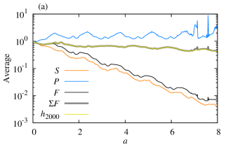
(a)

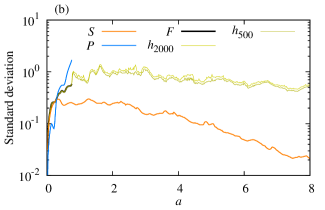
(b)

Figure 10: (a) The average and (b) the standard deviation, as a function of the accumulation depth $a$, of the indicated quantities. $W=0.6$ is kept constant, as well as the amplitude $A=0.25$ of the shear flow.

The chaotic example is presented in Fig. 10 (we note that individual spikes in the plots for $a>6$ are numerical artefacts due to the presence of caustics). Fig. 10a indicates that both $\langle\mathcal{S}\rangle$ and $\langle\mathcal{F}\rangle$ decrease exponentially as a function of the depth $a$. For the stretching, this can be regarded as a direct consequence of chaos, taking into account that depth is roughly proportional to settling time. The average $\langle\mathcal{P}\rangle$ of the projection factor increases only moderately (possibly related to saturational effects), and this is why the stretching behavior determines the total factor, resulting in an exponential dependence. Still, if we sum up the total factor over line branches, its average $\langle\sum\mathcal{F}\rangle$ remains approximately constant (see the gray line in Fig. 10a) because of mass conservation. That is, in spite of the strong reshapement of the material line, there is no net densification or much net dilution. Only a slight dilution is observable, for larger $a$, when the flow is able to advect parts of the material line horizontally farther away from the unit-sized horizontal section in which it was initialized. Calculating the average $\langle h_{N}\rangle$ of the normalized histogram $h_{N}$ yields the same result as $\langle\sum\mathcal{F}\rangle$ (for a wide range of bin numbers $N$, of which only one is shown), except for the absence of the artificial individual spikes.

As for the inhomogeneities, Fig. 10b shows that the total factor $\mathcal{F}$ exhibits an increasing inhomogeneity with increasing depth $a$, for small $a$, with a slight slowing down in the rate before the first caustics appear and it is not meaningful to continue the graph. This behavior seems to result from those of the stretching factor $\mathcal{S}$ and the projection factor $\mathcal{P}$, with equal importance. In particular, the standard deviation of the projection factor $\mathcal{P}$ is also increasing as long as it exists, due to the access to more and more different degrees of tiltness. Since different parts of the (phase) space are stretched differently, an even sharper increase is observable at the very beginning for the stretching factor $\mathcal{S}$, too. This increase, however, levels off very soon, and then turns to a pronounced decrease. This might be related to the decreasing magnitude of the factor $\mathcal{S}$ itself in average, but also to the stretching of any given part of the line being influenced by more and more parts of the (phase) space, more and more homogeneously. Maybe this mixing is why the standard deviation of the normalized histogram $h_{N}$ also starts decreasing for deeper depths $a$, for any particular choice $N$ of the coarse-graining (though taking on slightly different values depending on the number $N$ of the bins). At the same time, the coarse-grained quantifier $h_{N}$ follows, of course, the behavior of the total factor $\mathcal{F}$ very accurately for small depths $a$, i.e., it detects the inhomogeneization, and does not depend on the choice of $N$.

To summarize, both in chaotic and regular settings (see Appendix L), the emergence of the inhomogeneities mostly takes place at the beginning of the settling process (observable for small accumulation depths $a$). As soon as caustics appear, the standard deviation diverges, but any given coarse-graining exhibits homogeneization on the long term (for large $a$).

It is important to point out that the number of the caustics, besides the usual fluctuations (which are present in any statistics of any quantity), increases without bounds: it increases linearly and exponentially as a function of the depth $a$ in the regular and the chaotic case, respectively, see Figs. 11a and 11b). This indicates that inhomogeneization always continues on infinitely small spatial scales, due to the perpetual mixing of the (phase) space.

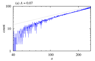
(a)

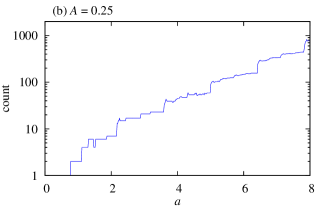
(b)

Figure 11: The number of the caustics, as a function of the accumulation depth $a$. For comparison, a linear law is shown in panel (a). $W=0.6$, and the amplitudes $A$ are as indicated.

V.3 Dependence on the amplitude $A$, and a balance between stretching and projection

Even in the presence of strong oscillations as a function of $a$, and of resonances as a function of $W$, the dependence on the amplitude $A$ of the shear flow can be investigated without being influenced by the spatial and temporal periodicities. We concentrate here on the factors $\mathcal{S}$, $\mathcal{P}$ and $\mathcal{F}$.

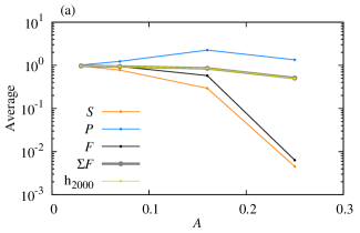
(a)

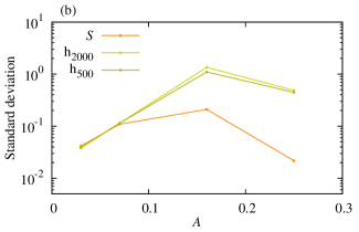
(b)

Figure 12: (a) The average and (b) the standard deviation, as a function of the amplitude $A$ of the shear flow, of the indicated quantites. $W=0.6$ is kept constant, as well as $\tau=12.5$.

As Fig. 12a illustrates, the average stretching factor $\langle\mathcal{S}\rangle$ exhibits a stronger response to increasing amplitude than the average projection factor $\langle\mathcal{P}\rangle$, resulting in a net dilution in the average total factor $\langle\mathcal{F}\rangle$. The projection factor $\langle\mathcal{P}\rangle$ actually saturates and even turns to a little (unexplained) weakening. Mass conservation keeps the total factor, when summed up over the different branches, approximately constant on average, with a slight dilution for larger $A$, like in Fig. 10a for larger $a$. In total, the dependences in Fig. 12a are remarkably similar to those in Fig. 10a (and Fig. 16a as well).

Due to the presence of caustics, only the stretching factor $\mathcal{S}$ and the coarse-grained normalized histograms $h_{N}$ are presented in Fig. 12b, which shows the standard deviations, and there is an inevitable dependence on $N$. Nevertheless, the matching with the corresponding figures showing the dependence on the depth (Figs. 10b and Fig. 16b) is also remarkably good. We conclude that increasing the amplitude $A$ has a similar effect as increasing the depth $a$, which is a consequence of a stronger rearrangement of the material in both cases.

Note in Fig. 12a that $\langle\mathcal{F}\rangle$ seems to tend to $1$ for decreasing $A$ more quickly than $\langle\mathcal{S}\rangle$ and $\langle\mathcal{P}\rangle$ themselves, and, in particular, it practically never goes above $1$. That is, for decreasing $A$ it might not be permitted to happen that projection would start to dominate stretching, even though this would be the inverse of what happens for increasing $A$. The prohibition of projection “winning” is also indicated by the experience that stretching and projection tend to be anticorrelated for decreasing $A$ (not shown, but cf. Fig. 3b and the related discussion). All this would mean that stretching and projection would become exactly balanced (cancelling out each other) in the limit of small $A$. The existence of this balancing limit would also imply that stretching and projection effects cannot occur without each other even for arbitrarily small perturbations of a uniform flow.

The existence of this balancing limit between stretching and projection, with a vanishing effect on the final density, might be a plausible assumption based on the observation that the horizontal displacements are much smaller than the vertical ones for the rather small amplitude $A$ of Figs. 3c-5c. Furthermore, taking into account the similar dependence on the amplitude $A$ and the depth $a$, and the smaller magnitude of $\langle\mathcal{F}\rangle$ in Figs. 10a and 16a than $\langle\mathcal{S}\rangle$ or $\langle\mathcal{P}\rangle$, a similar balancing might also occur for small depths $a$. However, note in Fig. 3b that stretching and projection do not cancel out each other locally in space, and Fig. 9b also suggests that stretching can be more important than projection in certain setups with weak mixing. As the reason for the anisotropy in the magnitudes of the relative displacements (e.g. in Figs. 3c-5c) is unexplained, we are not able to draw solid conclusions about the existence of a balancing limit between stretching and projection.

VI Discussion and conclusion

In this paper, we have described the mechanisms, stretching and projection, that give rise to inhomogeneities in the density of a layer of noninertial particles when the particles, after falling in a $d$-dimensional fluid flow (such that the particle velocity field is incompressible), are accumulated on a particular level. We have explored in an example flow how different characteristics of the accumulated density depend on generic parameters.

In order to check if our numerical observations are generic, we carried out the main analyses in a different example flow, a spatially periodic sheared vortex flow with temporal modulation Feudel et al. (2005); Lindner and Donner (2017). Considering a completely chaotic case in the presence of temporally periodic modulation, we found all of our qualitative conclusions to hold. What is even more important, breaking temporal periodicity did not introduce any relevant alteration.

The emergence of inhomogeneities from a homogeneous distribution, pointed out in this context first in Monroy et al. (2017), might be surprising in volume-preserving flows. In the special setting when the initial conditions are distributed in a $(d-1)$-dimensional subset of the $d$-dimensional domain of the fluid flow, the $(d-1)$-dimensional density defined along the evolving subset is not conserved. However, this fact cannot be regarded as the basic source of inhomogeneity. If we have a full-dimensional set of initial conditions, distributed over a continuous range of levels, we can apply the results of this paper to the horizontal layers, and then integrate over the initial vertical coordinate to obtain the final, $(d-1)$-dimensional density after the accumulation — and inhomogeneities arising within the individual layers are expected to be carried over to this final density. As a conclusion, we can say that the finite support of an (otherwise homogeneous) initial distribution is at the origin of the observed inhomogeneities at the accumulation level (without any coarse-graining, cf. Section I), but the mechanism by which they develop involves the stretching and the projection processes described above.

To illustrate the above considerations, we first show that a $2$-dimensional set of initial conditions in the $2$-dimensional shear flow problem (see Section IV.1) also leads to inhomogeneities in the accumulated density. In particular, we distribute $10\,201$ initial conditions on a uniform grid in a small square, $(x_{0},z_{0})\in[0.4,0.6]\times[-0.1,0.1]$. We numerically approximate the resulting accumulated density by calculating a normalized histogram $h$, which is shown in Fig. 13 and is clearly inhomogeneous. For comparison, we also include the total factors $\mathcal{F}$ (not summed up over the different branches) that come from the lowest and the highest rows of the initial square ($z_{0}=-0.1$ and $0.1$, respectively), as well as that corresponding to the total factor in Fig. 5b, which is obtained with the same parameters but from a horizontal line segment of unit length at $z_{0}=0$. The factors from the lowest and the highest rows of the initial square closely embrace the factor from Fig. 5b, exhibiting similar features (e.g. the caustics). The final density corresponding to the full square, as a function of the position, shows a similar shape to those of the individual factors, but the fine-scale structures are smeared out. In particular, all caustics disappear. Although this final density has a character different from those of the total factors of the individual lines, we can still say that the mechanisms leading to the final shape are strongly related to those (stretching and projection) that work for the individual lines.

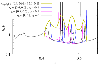
Figure 13: The normalized histogram $h$ resulting from the small square $(x_{0},z_{0})\in[0.4,0.6]\times[-0.1,0.1]$ of initial conditions (green), the total factor $\mathcal{F}$ corresponding to the lowest and the highest rows of the small square ($z_{0}=-0.1$ and $0.1$, blue and magenta, respectively), and the total factor $\mathcal{F}$ corresponding to an initial line segment of unit length at $z_{0}=0$ (the black line of Fig. 5b, black here, too), as a function of the position along the accumulation level. The bin size of the histogram is $0.01$. $A=0.06$, $W=0.6$, $a=97.2$.

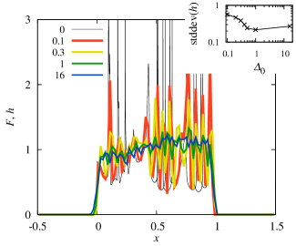
Figure 14: The normalized histogram $h$, as a function of the position along the accumulation level, resulting from rectangles of initial conditions with $(x_{0},z_{0})\in[0,1]\times[0,\Delta_{0}]$, where $\Delta_{0}$ is the thickness of the rectangle. The bin size of the histogram is $0.02$. Inset: the standard deviation of $h$ along the accumulation level, as a function of the thickness $\Delta_{0}$. $A=0.06$, $W=0.6$, $a=97.2$.

In Fig. 14 a sequence of densities is obtained from increasingly thicker layers of initial conditions (each having a unit horizontal width, $x_{0}\in[0,1]$) for the same parameter setting as in Fig. 13. When the initial thickness $\Delta_{0}$ is $0$, we recover the total factor in Fig. 5b with strong inhomogeneities, including caustics. When increasing the thickness, the caustics immediately disappear (i.e., no caustics can exist for any nonzero thickness), but all other inhomogeneities are smoothed out gradually. We obtain a rather homogeneous final horizontal density $\sigma_{\parallel}$ for $\Delta_{0}=1$, which does not change much for a much larger thickness of $\Delta_{0}=16$. The standard deviation of the final horizontal density, given in the inset of Fig. 14, decreases as a function of the initial thickness $\Delta_{0}$ for small thickness values, while it levels off for larger values, presumably as a result of the slow smearing out of the initially step-like distribution. We have thus confirmed that a finite initial support, smaller than (or, at most, comparable to) the characteristic length scale of the flow (being unity in Fig. 14), is needed for inhomogeneities to emerge from an initially homogeneous distribution within its support. Note that a reduced dimensionality or a finite support of the subset in which the initial conditions are distributed represents a strong inhomogeneity itself, but stretching and projection, determined by the geometry of the flow, give rise to additional inhomogeneities.

More generally, we can say that some kind of inhomogeneity is required in the initial distribution, but the advection in the flow introduces modifications to this distribution, and these modifications are characteristic to the geometry of the flow. For initial distributions with a full-dimensional ($d$-dimensional) support, stretching and projection are still the two mechanisms that modify the distribution. For generic shapes of the initial support, we expect the properties to be the most closely related to stretching and projection of those $(d-1)$-dimensional (hyper-) surfaces that are aligned with the unstable foliation of the phase space from the beginning. For initial supports with a small extension in a particular direction, stretching and projection of a $(d-1)$-dimensional (hyper-) surface perpendicular to this direction is expected to provide with a good approximation.

The relevance of stretching and projection also extends to the case when $v_{z}>0$ is allowed, which has not been investigated here. For this case, our results can be generalized by taking the first intersection of the investigated trajectories with the accumulation surface, and formally extending the accumulation to infinitely long times. A special property of such a setup is the typical presence of a chaotic saddle Lai and Tél (2011) in the domain of the flow, the unstable manifold of which may leave an important imprint on the particular shape of the distribution that is observed on the accumulation surface.

However, note that the unstable manifold gets importance for time scales of increasing duration, and its properties become actually observable for asymptotically long times. As discussed in Section I, relevant time scales in our motivating example are much shorter than asymptotically long ones, and our investigation in Sections IV-V revealed interesting phenomenology before reaching asymptotic behavior.

The study of dynamical systems has traditionally concentrated on asymptotically long time scales Ott (1993), even in open systems Lai and Tél (2011). The motivation for studying this regime probably has its roots in equilibrium statistical physics, in which any macroscopic time scale is infinitely long compared to the characteristic time scales of the individual components of the system. A common argument, furthermore, is that long-term behavior dominates observations of the system as opposed to short-term transients. Our study underlines the practical relevance of non-asymptotic behavior, which can exhibit remarkably rich phenomenology Ottino (1989); Pierrehumbert and Yang (1993).

A natural next step is the application of our results to a realistic oceanic setting to study the sedimentation of biogenic particles. From a theoretical point of view, the corresponding novelties are the anisotropy of the velocity field (cf. Section II.1) and its nonperiodic dependence on time. For a complete description, biogeochemical reactions and (dis)aggregation processes of the particles may need to be taken into account. Once all relevant ingredients are incorporated, the results should be useful to interpret instrumentally observed data, e.g. from sediment traps, as well.

Appendix A Justification of the particle equation of motion, Eq. (4)

Starting from the Maxey–Riley–Gatignol equations describing the motion of small particles in a flow, and for small enough values of the Stokes number $\mathrm{St}$, it can be shownHaller and Sapsis (2008) that, after a short transient time (of order $\mathrm{St}$), the particle dynamics approaches a slow manifold on which the particle position $\mathbf{X}$ is described, to first order in $\mathrm{St}$, by

$$\dot{\mathbf{X}}=\mathbf{v}_{\mathrm{fluid}}(\mathbf{X},t)+\mathrm{St}(\beta-1)\left(\frac{\mathrm{D}\mathbf{v}_{\mathrm{fluid}}}{\mathrm{D}t}+\frac{1}{\mathrm{Fr}^{2}}\hat{\mathbf{k}}\right),$$ (30)

where $\mathbf{v}_{\mathrm{fluid}}$ is the nondimensionalized velocity field of the fluid flow, $\mathrm{D}/\mathrm{D}t$ denotes the advective derivative following the fluid velocity, with $\mathrm{D}\mathbf{v}_{\mathrm{fluid}}/\mathrm{D}t$ describing particle inertia, and $\mathbf{k}$ is the vertical unit vector pointing upwards (in the $z$ direction).

In case $\mathrm{St}$ is very small, it may justify the complete neglection of the first-order term in $\mathrm{St}$ in (30). However, if $\mathrm{Fr}$ is considerably smaller than unity such that $\mathrm{St}\ll\mathrm{St}/\mathrm{Fr}^{2}\ll 1$, the gravitational term $\hat{\mathbf{k}}/\mathrm{Fr}^{2}$ may not be negligible even if the inertial term $\mathrm{D}\mathbf{v}_{\mathrm{fluid}}/\mathrm{D}t$ is. This situation leads to the well-knownSiegel and Deuser (1997); Siegel, Fields, and Buesseler (2008); Qiu, Doglioli, and Carlotti (2014); Roullier et al. (2014); Monroy et al. (2017) approximation

$$\dot{\mathbf{X}}=\mathbf{v}(\mathbf{X},t)\equiv\mathbf{v}_{\mathrm{fluid}}(\mathbf{X},t)-W\hat{\mathbf{k}}\ .$$ (31)

In cases, however, when $\mathrm{Fr}$ is so small that even $\mathrm{St}/\mathrm{Fr}^{2}\ll 1$ does not hold, the perturbative derivation of Eq. (30) is invalid. Nevertheless, in such circumstances it is straightforward to amend the derivation by Haller and SapsisHaller and Sapsis (2008) by considering the regime $\mathrm{St}\to 0$ and $\mathrm{Fr}\to 0$ with the dimensionless terminal settling velocity of a particle in still fluid, $W=(1-\beta)\mathrm{St}/\mathrm{Fr}^{2}$ (Eq. (3)), remaining constant. In this situation, for small enough values of $\mathrm{St}$, a normally hyperbolic slow manifold still exists, which is globally attracting, and in which the motion is described, to first order in $\mathrm{St}$, by

$$\dot{\mathbf{X}}=\mathbf{v}_{\mathrm{fluid}}(\mathbf{X},t)-W\hat{\mathbf{k}}+\mathrm{St}\left((\beta-1)\frac{\mathrm{D}\mathbf{v}_{\mathrm{fluid}}}{\mathrm{D}t}+W\hat{\mathbf{k}}\cdot\nabla\mathbf{v}_{\mathrm{fluid}}\right)\ .$$ (32)

For very small $\mathrm{St}$, when it is appropriate to neglect the first-order term in $\mathrm{St}$ in Eq. (32), we recover Eq. (31), which is also Eq. (4) of the main text. We thus conclude that whenever $\mathrm{St}\ll 1$ and $\mathrm{St}\ll W\sim\mathrm{St}/\mathrm{Fr}^{2}$, irrespectively of whether $W\sim\mathrm{St}/\mathrm{Fr}^{2}\ll 1$ or not, Eq. (4) is a good approximation. From a physical point of view, $\mathrm{St}\ll W$, or, equivalently, $1/\mathrm{Fr}^{2}\gg 1$ means that gravity is strong.

As discussed in Section II.1, $\mathrm{St}$ is typically very small for the type of particles we are interested in within a broad range of scales of oceanic flows, but $\mathrm{Fr}$ is very small as well under the same circumstances, so that $\mathrm{St}\ll 1$ and $\mathrm{St}\ll W\sim\mathrm{St}/\mathrm{Fr}^{2}$ are both satisfied. Therefore, according to our conclusion above, Eq. (4) provides with the relevant approximation, whether or not $W\sim\mathrm{St}/\mathrm{Fr}^{2}$ is small compared to unity (although it is typically not in our motivating situation, as mentioned in the main text).

Appendix B The derivation of Eqs. (5)-(7)

For this derivation, we introduce the notation $\mathrm{d}^{d-1}\mathbf{S}$ for integrations over $d-1$-dimensional (hyper-) surfaces when no parameterization is specified. Integrations over $d$-dimensional volumes are denoted by $\mathrm{d}^{d}\mathbf{X}$.

The surface density $\sigma_{\parallel}$ at a given point $\mathbf{x}$, with $z=-a$, of the accumulation level accumulated up to some time instant $t$ from the time of initialization $t_{0}$, can be computed from the mass that has crossed the accumulation level at $\mathbf{x}$:

$$\sigma_{\parallel}(\mathbf{x},t;t_{0})=\lim_{|S_{B}|\to 0}\frac{1}{|S_{B}|}\int^{t}_{t_{0}}\int_{S_{B}}\rho(t^{\prime},\mathbf{X})\mathbf{v}(t^{\prime},\mathbf{X})\cdot\mathrm{d}^{d-1}\mathbf{S}\mathrm{d}t^{\prime},$$ (33)

where $S_{B}$ is a surface in the neighborhood of $\mathbf{x}$ within the accumulation level (defined by $z=-a$), and $\rho(t,\mathbf{X})$ is the full-dimensional density.

Let us consider all trajectories, initialized at $z=z_{0}$, that arrive at the accumulation level within $S_{B}$. We denote by $S$ the (hyper-) surface that encloses all these trajectories from their initialization to $z=-a$. Since the density is assumed to be the constant zero above $z=z_{0}$, and trajectories do not cross the side of the surface $S$ by definition, we can extend the domain of integration from $S_{B}$ to $S$ in (33):

$$\sigma_{\parallel}(\mathbf{x},t;t_{0}) =\lim_{|S_{B}|\to 0}\frac{1}{|S_{B}|}\int^{t}_{t_{0}}\int_{S}\rho(t^{\prime},\mathbf{X})\mathbf{v}(t^{\prime},\mathbf{X})\cdot\mathrm{d}^{d-1}\mathbf{S}\mathrm{d}t^{\prime}$$

$$=\lim_{|S_{B}|\to 0}\frac{1}{|S_{B}|}\int^{t}_{t_{0}}\int_{V}\frac{\partial}{\partial\mathbf{X}^{\prime}}\cdot(\rho(t^{\prime},\mathbf{X}^{\prime})\mathbf{v}(t^{\prime},\mathbf{X}^{\prime}))\mathrm{d}^{d}\mathbf{X}^{\prime}\mathrm{d}t^{\prime},$$ (34)

where we have used the divergence theorem, and $V$ is the $d$-volume enclosed by $S$. Using the mass conservation expressed by the continuity equation

$$\frac{\partial\rho(t,\mathbf{X})}{\partial t}=-\frac{\partial}{\partial\mathbf{X}}\left(\rho(t,\mathbf{X})\mathbf{v}(t,\mathbf{X})\right),$$ (35)

we obtain

$$\sigma_{\parallel}(\mathbf{x},t;t_{0})=-\lim_{|S_{B}|\to 0}\frac{1}{|S_{B}|}\int^{t}_{t_{0}}\int_{V}\frac{\partial\rho(t^{\prime},\mathbf{X}^{\prime})}{\partial t^{\prime}}\mathrm{d}^{d}\mathbf{X}^{\prime}\mathrm{d}t^{\prime},$$ (36)

For a fixed volume, we can take the partial derivative outside the spatial integral as a total derivative:

$$\sigma_{\parallel}(\mathbf{x},t;t_{0}) =-\lim_{|S_{B}|\to 0}\frac{1}{|S_{B}|}\int^{t}_{t_{0}}\frac{\mathrm{d}}{\mathrm{d}t^{\prime}}\int_{V}\rho(t^{\prime},\mathbf{X}^{\prime})\mathrm{d}^{d}\mathbf{X}^{\prime}\mathrm{d}t^{\prime}$$

$$=\lim_{|S_{B}|\to 0}\frac{1}{|S_{B}|}\left(\int_{V}\rho(t_{0},\mathbf{X}^{\prime})\mathrm{d}^{d}\mathbf{X}^{\prime}-\int_{V}\rho(t,\mathbf{X}^{\prime})\mathrm{d}^{d}\mathbf{X}^{\prime}\right).$$ (37)

For sufficiently large $t$, i.e., after the arrival of all trajectories within $V$ to the accumulation level, the second term in (37) vanishes (the trajectories have already crossed the accumulation level). In the limit $|S_{B}|\to 0$ we only have one trajectory within $V$, which arrives to the accumulation level at the point $\mathbf{x}$, and the preimage of which at $t=t_{0}$ we denote by $\mathbf{x}_{0}$ at $z=z_{0}$. In this limit, the “sufficiently large” $t$ is $t\geq t(f_{z}=-a,\mathbf{x}_{0})$, and $\sigma_{\parallel}(\mathbf{x},t\geq t(f_{z}=-a,\mathbf{x}_{0});t_{0})$ is what was denoted in Section III.1 as $\sigma_{\parallel}(t(f_{z}=-a,\mathbf{x}_{0}),\mathbf{x}_{0})$. As for the first term in (37), it is the total initial mass within $V$, which can be, again in the limit $|S_{B}|\to 0$, written as the product of the initial surface density $\sigma(t=t_{0};\mathbf{x}_{0})$ at $\mathbf{x}_{0}$ and the area $|S_{U}|$ of the infinitesimal surface $S_{U}$ at $z=z_{0}$ that corresponds to the trajectories arriving at $z=-a$ within $S_{B}$. For some given $\mathbf{x}_{0}$, we can thus write:

$$\sigma_{\parallel}(t(f_{z}=-a,\mathbf{x}_{0}),\mathbf{x}_{0})=\lim_{|S_{B}|\to 0}\frac{1}{|S_{B}|}\sigma(t=t_{0};\mathbf{x}_{0})|S_{U}|.$$ (38)

Since $\sigma(t=t_{0};\mathbf{x}_{0})$ itself is unaffected by the limit, (38) is the same as (5) with

$$\mathcal{F}(t(f_{z}=-a,\mathbf{x}_{0}),\mathbf{x}_{0})=\lim_{|S_{B}|\to 0}\frac{|S_{U}|}{|S_{B}|},$$ (39)

that is, the total factor is just the ratio of the areas of the initial and the final infinitesimal surfaces, one image of the other, neighboring horizontally (with $z=z_{0}$ and $z=-a$) the starting and the endpoint of the trajectory, respectively.

We are now looking for the mathematical relation linking these areas. This relation is provided by the transformation of the coordinates from those of the initial surface to those of the final one:

$$|S_{B}| =\int_{S_{B}}\mathrm{d}^{d-1}\mathbf{S}=\int_{S_{B}}\mathrm{d}^{d-1}\mathbf{x}$$

$$=\int_{S_{U}}\det\left(\left.\frac{\partial(f_{1}(t(f_{z}=-a,\mathbf{x}_{0}),\mathbf{x}_{0}),\ldots,f_{d-1}(t(f_{z}=-a,\mathbf{x}_{0}),\mathbf{x}_{0}))}{\partial\mathbf{x}_{0}}\right|_{f_{z}}\right)\mathrm{d}^{d-1}\mathbf{x}_{0}.$$ (40)

Substituting this and $|S_{U}|=\int_{S_{U}}\mathrm{d}^{d-1}\mathbf{S}=\int_{S_{U}}\mathrm{d}^{d-1}\mathbf{x}_{0}$ into (39), we recover (6)-(7) in the indicated limit.

Appendix C The derivation of Eq. (8)

Let us compare two forms of the total differential of the horizontal position of the endpoint of a trajectory:

$$\mathrm{d}f_{i}(t,\mathbf{x}_{0}) =\sum_{j=1}^{d-1}\left.\frac{\partial f_{i}(t,\mathbf{x}_{0})}{\partial x_{0j}}\right|_{t}\mathrm{d}x_{0j}+\left.\frac{\partial f_{i}(t,\mathbf{x}_{0})}{\partial t}\right|_{\mathbf{x}_{0}}\mathrm{d}t,$$ (41)

$$\mathrm{d}f_{i}(t(f_{z},\mathbf{x}_{0}),\mathbf{x}_{0}) =\sum_{j=1}^{d-1}\left.\frac{\partial f_{i}(t(f_{z},\mathbf{x}_{0}),\mathbf{x}_{0})}{\partial x_{0j}}\right|_{f_{z}}\mathrm{d}x_{0j}+\left.\frac{\partial f_{i}(t(f_{z},\mathbf{x}_{0}),\mathbf{x}_{0})}{\partial f_{z}}\right|_{\mathbf{x}_{0}}\mathrm{d}f_{z}$$ (42)

for $i\in\{1,\ldots,d-1\}$. For (41), the independent variables are $t$ and $\mathbf{x}_{0}$, while for (42), they are $f_{z}$ and $\mathbf{x}_{0}$ (cf. Section III.1). Similarly to (41), we can write the total differential of $f_{z}$ itself as follows:

$$\mathrm{d}f_{z}(t,\mathbf{x}_{0})=\sum_{j=1}^{d-1}\left.\frac{\partial f_{z}(t,\mathbf{x}_{0})}{\partial x_{0j}}\right|_{t}\mathrm{d}x_{0j}+\left.\frac{\partial f_{z}(t,\mathbf{x}_{0})}{\partial t}\right|_{\mathbf{x}_{0}}\mathrm{d}t.$$ (43)

Substituting (43) into (42) and comparing the result with (41), which must be equal to (42), gives

$$\left.\frac{\partial f_{i}(t,\mathbf{x}_{0})}{\partial x_{0j}}\right|_{t} =\left.\frac{\partial f_{i}(t(f_{z},\mathbf{x}_{0}),\mathbf{x}_{0})}{\partial x_{0j}}\right|_{f_{z}}+\left.\frac{\partial f_{i}(t(f_{z},\mathbf{x}_{0}),\mathbf{x}_{0})}{\partial f_{z}}\right|_{\mathbf{x}_{0}}\left.\frac{\partial f_{z}(t,\mathbf{x}_{0})}{\partial x_{0j}}\right|_{t},$$ (44)

$$\left.\frac{\partial f_{i}(t,\mathbf{x}_{0})}{\partial t}\right|_{\mathbf{x}_{0}} =\left.\frac{\partial f_{i}(t(f_{z},\mathbf{x}_{0}),\mathbf{x}_{0})}{\partial f_{z}}\right|_{\mathbf{x}_{0}}\left.\frac{\partial f_{z}(t,\mathbf{x}_{0})}{\partial t}\right|_{\mathbf{x}_{0}}.$$ (45)

for all $i,j\in\{1,\ldots,d-1\}$. Taking into account in (45) that, along a given trajectory characterized by $\mathbf{x}_{0}$,

$$\left.\frac{\partial f_{i}(t,\mathbf{x}_{0})}{\partial t}\right|_{\mathbf{x}_{0}}=v_{i}(t,\mathbf{f}(t,\mathbf{x}_{0}))$$ (46)

for $i\in\{1,\ldots,d\}$, substituting $\left.\frac{\partial f_{i}(t(f_{z},\mathbf{x}_{0}),\mathbf{x}_{0})}{\partial f_{z}}\right|_{\mathbf{x}_{0}}$ from (45) into (44) yields (8).

Appendix D The derivation of Eq. (9)

According to a Jacobi-type formula Harville (2008),

$$|J^{-1}|\frac{\partial|J|}{\partial\alpha}=\mathrm{Tr}\,\left(\frac{\partial J}{\partial\alpha}J^{-1}\right),$$ (47)

where $\alpha$ can be an arbitrary variable. We shall choose $\alpha=f_{z}$, and solve the differential equation (47) for $|J|$ for a fixed $\mathbf{x}_{0}$ (i.e., “along a trajectory”). In order to do this, we shall transform the right-hand side of (47) to express it in terms of the velocity field.

We first introduce a new quantity, the derivative of the final position $\mathbf{f}$ with respect to the vertical coordinate $f_{z}$:

$$\tilde{v}_{i}(t(f_{z},\mathbf{x}_{0}),\mathbf{x}_{0}) =\left.\frac{\partial f_{i}(t(f_{z},\mathbf{x}_{0}),\mathbf{x}_{0})}{\partial f_{z}}\right|_{\mathbf{x}_{0}}$$

$$=\left.\frac{\partial f_{i}(t,\mathbf{x}_{0})}{\partial t}\right|_{\mathbf{x}_{0},t=t(f_{z},\mathbf{x}_{0})}\left.\frac{\partial t(f_{z},\mathbf{x}_{0})}{\partial f_{z}}\right|_{\mathbf{x}_{0}}$$

$$=\frac{v_{i}(t(f_{z},\mathbf{x}_{0}),\mathbf{f}(t(f_{z},\mathbf{x}_{0}),\mathbf{x}_{0}))}{v_{z}(t(f_{z},\mathbf{x}_{0}),\mathbf{f}(t(f_{z},\mathbf{x}_{0}),\mathbf{x}_{0}))},$$ (48)

for $i\in\{1,\ldots,d\}$ — that is, our new quantity $\tilde{\mathbf{v}}$ is simply a rescaled version of the original velocity $\mathbf{v}$.

Now let us perform a change in the variables: in a sufficiently small neighborhood of a given trajectory (characterized by $\mathbf{x}_{0}$), let us regard the coordinates $\mathbf{f}=(f_{1},\ldots,f_{d})$ of the endpoint of the trajectory as independent variables, instead of $\mathbf{x}_{0}$ and $f_{z}$ — then $\mathbf{x}_{0}$ becomes a function of $\mathbf{f}$, $\mathbf{x}_{0}=\mathbf{x}_{0}(\mathbf{f})$. This change is possible only in a local sense, since the function $\mathbf{f}=\mathbf{f}(t(f_{z},\mathbf{x}_{0}),\mathbf{x}_{0})$ is not invertible, but we can usually find a small neighborhood around a given trajectory where it is. The exceptions are trajectories for which $\det(J)=0$. For such trajectories, the factor $\mathcal{F}$ tends to infinity (the positions $\mathbf{f}$ of the endpoints of these trajectories correspond to those of the caustics, cf. Section III.2, and (21) and (24) in particular), so that the computation of $\mathcal{F}$ becomes irrelevant.

In terms of the new independent variables, let us take the horizontal part of the divergence of the rescaled velocity $\tilde{\mathbf{v}}$, while keeping $f_{z}$ constant (note that this implies the variation of $\mathbf{x}_{0}$, cf. the discussion below):

$$\sum_{i=1}^{d-1}\left.\frac{\partial}{\partial f_{i}}\tilde{v}_{i}(t(f_{z},\mathbf{x}_{0}(\mathbf{f})),\mathbf{x}_{0}(\mathbf{f}))\right|_{f_{z}} =\sum_{i,j=1}^{d-1}\left(\left.\frac{\partial\tilde{v}_{i}(t(f_{z},\mathbf{x}_{0}),\mathbf{x}_{0})}{\partial x_{0j}}\right|_{f_{z},\mathbf{x}_{0}=\mathbf{x}_{0}(\mathbf{f})}\left.\frac{\partial x_{0j}(\mathbf{f})}{\partial f_{i}}\right|_{f_{z}}\right)$$

$$=\sum_{i,j=1}^{d-1}\left(\left.\frac{\partial\left(\left.\frac{\partial f_{i}(t(f_{z},\mathbf{x}_{0}),\mathbf{x}_{0})}{\partial f_{z}}\right|_{\mathbf{x}_{0},\mathbf{x}_{0}=\mathbf{x}_{0}(\mathbf{f})}\right)}{\partial x_{0j}}\right|_{f_{z},\mathbf{x}_{0}=\mathbf{x}_{0}(\mathbf{f})}\left.\frac{\partial x_{0j}(\mathbf{f})}{\partial f_{i}}\right|_{f_{z}}\right)$$

$$=\sum_{i,j=1}^{d-1}\left(\left.\frac{\partial\left(\left.\frac{\partial f_{i}(t(f_{z},\mathbf{x}_{0}),\mathbf{x}_{0})}{\partial x_{0j}}\right|_{f_{z},\mathbf{x}_{0}=\mathbf{x}_{0}(\mathbf{f})}\right)}{\partial f_{z}}\right|_{\mathbf{x}_{0},\mathbf{x}_{0}=\mathbf{x}_{0}(\mathbf{f})}\left.\frac{\partial x_{0j}(\mathbf{f})}{\partial f_{i}}\right|_{f_{z}}\right),$$ (49)

where we applied the chain rule in the first line, substituted (48) for the second line, and, for the third line, took advantage of the fact that the partial derivative is taken at a constant $f_{z}$. If it were taken at a constant time $t$, changing the order of the derivations would not be possible. What we obtain in the third line of (49) is exactly the right-hand side of (47). After changing the independent variables back to $\mathbf{x}_{0}$ and $f_{z}$, and substituting (49) into (47), we can solve the differential equation in terms of $f_{z}$, keeping $\mathbf{x}_{0}$ constant, which corresponds to following one particular trajectory. With the initial condition that $|J|$ is the identity matrix for $f_{z}=z_{0}$, we obtain (9), for which we introduce a new notation. In particular, due to the different role of $f_{z}$ compared to the horizontal components of the endpoint $\mathbf{f}$ of the trajectory, we find it useful to introduce the vector $\mathbf{f}_{\parallel}=(f_{1},\ldots,f_{d-1})$, composed of the horizontal coordinates of the trajectory. At a constant $f_{z}$ (or at a constant $t$, as in Appendix F), it is $\mathbf{f}_{\parallel}$ that identifies the particular trajectory, this is why the variation of $\mathbf{f}_{\parallel}$ at a constant $f_{z}$ (or $t$) implies the variation of $\mathbf{x}_{0}$.

Appendix E Transforming Eq. (9)

In this Appendix, we collect the results for how Eq. (9) can be transformed and evaluated numerically, and discuss the derivations in further appendices.

As shown in Appendix F, Eq. (9) can be written with derivatives taken at a constant time $t$:

$$\mathcal{F}(t(f_{z}=-a,\mathbf{x}_{0}),\mathbf{x}_{0})= \exp\left(-\int_{t_{0}}^{t(f_{z}=-a,\mathbf{x}_{0})}\sum_{i=1}^{d-1}\left[\left.\frac{\partial v_{i}(t,\mathbf{f}(t,\mathbf{x}_{0}(t,\mathbf{f}_{\parallel})))}{\partial f_{i}}\right|_{t,\mathbf{f}_{\parallel}=\mathbf{f}_{\parallel}(t,\mathbf{x}_{0})}\right.\right.$$

$$-\left.\left.\left.\frac{\partial v_{z}(t,\mathbf{f}(t,\mathbf{x}_{0}(t,\mathbf{f}_{\parallel})))}{\partial f_{k}}\right|_{t,\mathbf{f}_{\parallel}=\mathbf{f}_{\parallel}(t,\mathbf{x}_{0})}\frac{v_{k}(t,\mathbf{f}(t,\mathbf{x}_{0}))}{v_{z}(t,\mathbf{f}(t,\mathbf{x}_{0}))}\right.\right.$$

$$+\left.\left.\frac{\left.\frac{\partial f_{z}(t,\mathbf{x}_{0}(t,\mathbf{f}_{\parallel}))}{\partial f_{i}}\right|_{t,\mathbf{f}_{\parallel}=\mathbf{f}_{\parallel}(t,\mathbf{x}_{0})}\left.\frac{\partial}{\partial t}\left(\frac{v_{i}(t,\mathbf{f}(t,\mathbf{x}_{0}))}{v_{z}(t,\mathbf{f}(t,\mathbf{x}_{0}))}\right)\right|_{f_{1},\ldots,f_{d-1}}}{\sum_{k=1}^{d-1}\left.\frac{\partial f_{z}(t,\mathbf{x}_{0}(t,\mathbf{f}_{\parallel}))}{\partial f_{i}}\right|_{t,\mathbf{f}_{\parallel}=\mathbf{f}_{\parallel}(t,\mathbf{x}_{0})}\frac{v_{i}(t,\mathbf{f}(t,\mathbf{x}_{0}))}{v_{z}(t,\mathbf{f}(t,\mathbf{x}_{0}))}-1}\right]\right),$$ (50)

where the derivatives taken with respect to the coordinates $f_{i}$, $i\in\{1,\ldots,d-1\}$, at a constant $t$ again correspond to varying $\mathbf{x}_{0}$, which implies that these derivatives are taken along the surface to which the initial sheet of particles evolves up to time $t$. The distinguishing property of this formula is that all of its components can be evaluated locally, except for $\left.\frac{\partial f_{z}(t,\mathbf{x}_{0}(t,\mathbf{f}_{\parallel}))}{\partial f_{i}}\right|_{t,\mathbf{f}_{\parallel}=\mathbf{f}_{\parallel}(t,\mathbf{x}_{0})}$. These latter quantities describe the tiltness of the surface, and they can be obtained by solving the following differential equation (see Appendix G for the derivation):

$$\frac{\mathrm{d}}{\mathrm{d}t}\left(\left.\frac{\partial f_{z}(t,\mathbf{x}_{0}(t,\mathbf{f}_{\parallel}))}{\partial f_{i}}\right|_{t}\right)= \left.\frac{\partial v_{z}(t,\mathbf{f}(t,\mathbf{f}_{\parallel})}{\partial x_{i}}\right|_{t}+\left.\frac{\partial f_{z}(t,\mathbf{x}_{0}(t,\mathbf{f}_{\parallel}))}{\partial f_{i}}\right|_{t}\left.\frac{\partial v_{z}(t,\mathbf{f}(t,\mathbf{f}_{\parallel})}{\partial z}\right|_{t}$$

$$- \sum^{d-1}_{j=1}\left(\left.\frac{\partial v_{j}(t,\mathbf{f}(t,\mathbf{f}_{\parallel}))}{\partial x_{i}}\right|_{t}+\left.\frac{\partial f_{z}(t,\mathbf{x}_{0}(t,\mathbf{f}_{\parallel}))}{\partial f_{i}}\right|_{t}\left.\frac{\partial v_{j}(t,\mathbf{f}(t,\mathbf{f}_{\parallel}))}{\partial z}\right|_{t}\right)\left.\frac{\partial f_{z}(t,\mathbf{x}_{0}(t,\mathbf{f}_{\parallel}))}{\partial f_{j}}\right|_{t},$$ (51)

with the initial condition $\left.\frac{\partial f_{z}(t,\mathbf{x}_{0}(t,\mathbf{f}_{\parallel}))}{\partial f_{i}}\right|_{t=t_{0},\mathbf{f}_{\parallel}=\mathbf{f}_{\parallel}(t=t_{0},\mathbf{x}_{0})}=0$. The solution can numerically be evaluated along any single trajectory.

It is important to note that typically, $\left.\frac{\partial f_{z}(t,\mathbf{x}_{0}(t,\mathbf{f}_{\parallel}))}{\partial f_{i}}\right|_{t,\mathbf{f}_{\parallel}=\mathbf{f}_{\parallel}(t,\mathbf{x}_{0})}\simeq 0$ in realistic oceanic flows, and neglecting the second and the third terms in (51) yields

$$\left.\frac{\partial f_{z}(t,\mathbf{x}_{0}(t,\mathbf{f}_{\parallel}))}{\partial f_{i}}\right|_{t,\mathbf{f}_{\parallel}=\mathbf{f}_{\parallel}(t,\mathbf{x}_{0})}\simeq\int_{t_{0}}^{t}\left.\frac{\partial v_{z}(t^{\prime},\mathbf{f}(t^{\prime},\mathbf{f}_{\parallel}=\mathbf{f}_{\parallel}(t^{\prime},\mathbf{x}_{0}))}{\partial x_{i}}\right|_{t^{\prime}}\mathrm{d}t^{\prime}.$$ (52)

Appendix F The derivation of Eq. (50)

First, the integral in (9) can be transformed to a temporal one as

$$\mathcal{F}(t(f_{z}=-a,\mathbf{x}_{0}),\mathbf{x}_{0})$$

$$=\exp\Bigg{(}-\int_{t_{0}}^{t(f_{z}=-a,\mathbf{x}_{0})}\sum_{i=1}^{d-1}\left.\frac{\partial}{\partial f_{i}}\left(\frac{\hat{v}_{i}(f_{z},\mathbf{f}_{\parallel})}{\hat{v}_{z}(f_{z},\mathbf{f}_{\parallel})}\right)\right|_{f_{z},f_{z}=f_{z}(t,\mathbf{x}_{0}),\mathbf{f}_{\parallel}=\mathbf{f}_{\parallel}(t,\mathbf{x}_{0}))}v_{z}(t,\mathbf{f}(t,\mathbf{x}_{0}))\mathrm{d}t\Bigg{)}.$$ (53)

In order to replace the derivatives taken at constant depth $f_{z}$ by derivatives that are taken at constant time $t$, we perform a calculation similar to that expressed by (41)-(45) in Appendix C for $\tilde{\mathbf{v}}$ instead of $\mathbf{f}$. We first recognize that we can regard $\mathbf{f}_{\parallel}=(f_{1},\ldots,f_{d-1})$ (the horizontal coordinates of a trajectory) and $t$ as independent variables, too, instead of $\mathbf{f}=(f_{1},\ldots,f_{d})$ (i.e., $\mathbf{f}_{\parallel}$ and $f_{z}$) as in Appendix D. We are interested here in the direct dependence of $\tilde{\mathbf{v}}$ on these new independent variables. To emphasize this, we introduce the notations $\hat{\tilde{\mathbf{v}}}(t,\mathbf{f}_{\parallel})$ and $\hat{\tilde{\mathbf{v}}}(f_{z},\mathbf{f}_{\parallel})$ in this Appendix instead of the more complicated notation $\tilde{\mathbf{v}}(t,\mathbf{x}_{0}(t,\mathbf{f}_{\parallel}))$ and $\tilde{\mathbf{v}}(t(f_{z},\mathbf{x}_{0}(f_{z},\mathbf{f}_{\parallel})),\mathbf{x}_{0}(f_{z},\mathbf{f}_{\parallel}))$, and we compare the total differential of $\hat{\tilde{\mathbf{v}}}$ expressed in terms of $t$ and $\mathbf{f}_{\parallel}$ and that expressed in terms of $f_{z}$ and $\mathbf{f}_{\parallel}$:

$$\mathrm{d}\hat{\tilde{v}}_{i}(t,\mathbf{f}_{\parallel}) =\sum_{j=1}^{d-1}\left.\frac{\partial\hat{\tilde{v}}_{i}(t,\mathbf{f}_{\parallel})}{\partial f_{j}}\right|_{t}\mathrm{d}f_{j}+\left.\frac{\partial\hat{\tilde{v}}_{i}(t,\mathbf{f}_{\parallel})}{\partial t}\right|_{\mathbf{f}_{\parallel}}\mathrm{d}t,$$ (54)

$$\mathrm{d}\hat{\tilde{v}}_{i}(f_{z},\mathbf{f}_{\parallel}) =\sum_{j=1}^{d-1}\left.\frac{\partial\hat{\tilde{v}}_{i}(f_{z},\mathbf{f}_{\parallel})}{\partial f_{j}}\right|_{f_{z}}\mathrm{d}f_{j}+\left.\frac{\partial\hat{\tilde{v}}_{i}(f_{z},\mathbf{f}_{\parallel})}{\partial f_{z}}\right|_{\mathbf{f}_{\parallel}}\mathrm{d}f_{z}$$ (55)

for $i\in\{1,\ldots,d-1\}$ (note that $\hat{\tilde{v}}_{z}=1$ is constant).

Before we can compare (54) and (55), we have to take into account that $f_{z}$ itself can be regarded as a function of our independent variables $\mathbf{f}_{\parallel}$ and $t$, hence

$$\mathrm{d}f_{z}(t,\mathbf{f}_{\parallel})=\sum_{j=1}^{d-1}\left.\frac{\partial f_{z}(t,\mathbf{f}_{\parallel})}{\partial f_{j}}\right|_{t}\mathrm{d}f_{j}+\left.\frac{\partial f_{z}(t,\mathbf{f}_{\parallel})}{\partial t}\right|_{\mathbf{f}_{\parallel}}\mathrm{d}t.$$ (56)

Substituting this into (54) and comparing the result with (55), we obtain

$$\left.\frac{\partial\hat{\tilde{v}}_{i}(t,\mathbf{f}_{\parallel})}{\partial f_{j}}\right|_{t} =\left.\frac{\partial\hat{\tilde{v}}_{i}(f_{z},\mathbf{f}_{\parallel})}{\partial f_{j}}\right|_{f_{z}}+\left.\frac{\partial\hat{\tilde{v}}_{i}(f_{z},\mathbf{f}_{\parallel})}{\partial f_{z}}\right|_{\mathbf{f}_{\parallel}}\left.\frac{\partial f_{z}(t,\mathbf{f}_{\parallel})}{\partial f_{j}}\right|_{t},$$ (57)

$$\left.\frac{\partial\hat{\tilde{v}}_{i}(t,\mathbf{f}_{\parallel})}{\partial t}\right|_{\mathbf{f}_{\parallel}} =\left.\frac{\partial\hat{\tilde{v}}_{i}(f_{z},\mathbf{f}_{\parallel})}{\partial f_{z}}\right|_{\mathbf{f}_{\parallel}}\left.\frac{\partial f_{z}(t,\mathbf{f}_{\parallel})}{\partial t}\right|_{\mathbf{f}_{\parallel}}$$ (58)

for $i,j\in\{1,\ldots,d-1\}$.

Still similarly to what is done in Section C, we can substitute $\left.\frac{\partial\hat{\tilde{v}}_{i}(f_{z},\mathbf{f}_{\parallel})}{\partial f_{z}}\right|_{\mathbf{f}_{\parallel}}$ from (58) into (57). Additionally, $\left.\frac{\partial f_{z}(t,\mathbf{f}_{\parallel})}{\partial t}\right|_{\mathbf{f}_{\parallel}}$ in (58) can be expressed based on (56). Namely, (56) can be written as

$$\frac{\mathrm{d}f_{z}(t,\mathbf{f}_{\parallel})}{\mathrm{d}t}=\sum_{j=1}^{d-1}\left.\frac{\partial f_{z}(t,\mathbf{f}_{\parallel})}{\partial f_{j}}\right|_{t}\frac{\mathrm{d}f_{j}}{\mathrm{d}t}+\left.\frac{\partial f_{z}(t,\mathbf{f}_{\parallel})}{\partial t}\right|_{\mathbf{f}_{\parallel}},$$ (59)

in which we can identify the velocities according to (46), but with total derivatives, if we exclude varying $\mathbf{x}_{0}$: this choice means that we are following particular trajectories, and the horizontal components $f_{j}$, $j\in\{1,\ldots,d-1\}$, become functions of the time $t$. In this way, we obtain

$$\left.\frac{\partial f_{z}(t,\mathbf{f}_{\parallel})}{\partial t}\right|_{\mathbf{f}_{\parallel}}=v_{z}(t,\mathbf{f}(t,\mathbf{f}_{\parallel}))-\sum_{j=1}^{d-1}\left.\frac{\partial f_{z}(t,\mathbf{f}_{\parallel})}{\partial f_{j}}\right|_{t}v_{j}(t,\mathbf{f}(t,\mathbf{f}_{\parallel})).$$ (60)

Taking this into account in (58) when substituting $\left.\frac{\partial\hat{\tilde{v}}_{i}(f_{z},\mathbf{f}_{\parallel})}{\partial f_{z}}\right|_{\mathbf{f}_{\parallel}}$ from (58) into (57), we obtain

$$\left.\frac{\partial\hat{\tilde{v}}_{i}(f_{z},\mathbf{f}_{\parallel})}{\partial f_{j}}\right|_{f_{z}}=\left.\frac{\partial\hat{\tilde{v}}_{i}(t,\mathbf{f}_{\parallel})}{\partial f_{j}}\right|_{t}-\frac{\left.\frac{\partial\hat{\tilde{v}}_{i}(t,\mathbf{f}_{\parallel})}{\partial t}\right|_{\mathbf{f}_{\parallel}}}{v_{z}(t,\mathbf{f}(t,\mathbf{f}_{\parallel}))-\sum_{k=1}^{d-1}\left.\frac{\partial f_{z}(t,\mathbf{f}_{\parallel})}{\partial f_{k}}\right|_{t}v_{k}(t,\mathbf{f}(t,\mathbf{f}_{\parallel}))}\left.\frac{\partial f_{z}(t,\mathbf{f}_{\parallel})}{\partial f_{j}}\right|_{t}$$ (61)

for $i,j\in\{1,\ldots,d-1\}$. Note that the derivatives taken at constant time $t$ with respect to $f_{j}$, $j\in\{1,\ldots,d-1\}$, correspond to varying the selected trajectory, as explained in Appendix D, so that these derivatives are not taken at a constant vertical coordinate: instead, they are taken along the surface to which the initial sheet of particles evolves up to time $t$.

Expanding the definition (48), (61) can be applied to express $\sum_{i=1}^{d-1}\left.\frac{\partial}{\partial f_{i}}\left(\frac{\hat{v}_{i}(f_{z},\mathbf{f}_{\parallel})}{\hat{v}_{z}(f_{z},\mathbf{f}_{\parallel})}\right)\right|_{f_{z},f_{z}=f_{z}(t,\mathbf{x}_{0}),\mathbf{f}_{\parallel}=\mathbf{f}_{\parallel}(t,\mathbf{x}_{0}))}$ in (53). After expanding the first term, simplification, and changing the variables from $t$ and $\mathbf{f}_{\parallel}$ to $t$ and $\mathbf{x}_{0}$, we recover (50).

Appendix G The derivation of Eq. (51)

In this derivation, we regard the quantities $f_{z}$ and $\left.\frac{\partial f_{z}(t,\mathbf{x}_{0}(t,\mathbf{f}_{\parallel}))}{\partial f_{i}}\right|_{t}$ to be functions of $t$ and $\mathbf{f}_{\parallel}$ (we express this by writing $f_{z}(t,\mathbf{f}_{\parallel})$ and $\left.\frac{\partial f_{z}(t,\mathbf{f}_{\parallel})}{\partial f_{i}}\right|_{t}$), and, as explained in relation with (60), we regard $\mathbf{f}_{\parallel}$ itself to be a function of $t$, which means that we choose to follow particular trajectories.

After applying the definition of the total derivative to $\left.\frac{\partial f_{z}(t,\mathbf{f}_{\parallel})}{\partial f_{i}}\right|_{t}$ (in terms of $t$ and $\mathbf{f}_{\parallel}$), we can make a rearrangement to obtain

$$\frac{\mathrm{d}}{\mathrm{d}t}\left(\left.\frac{\partial f_{z}(t,\mathbf{f}_{\parallel})}{\partial f_{i}}\right|_{t}\right)= \frac{\partial}{\partial f_{i}}\left.\left(\left.\frac{\partial f_{z}(t,\mathbf{f}_{\parallel})}{\partial t}\right|_{\mathbf{f}_{\parallel}}+\sum^{d-1}_{j=1}v_{j}(t,\mathbf{f}(t,\mathbf{f}_{\parallel}))\left.\frac{\partial f_{z}(t,\mathbf{f}_{\parallel})}{\partial f_{j}}\right|_{t}\right)\right|_{t}$$

$$-\sum^{d-1}_{j=1}\left.\frac{\partial v_{j}(t,\mathbf{f}(t,\mathbf{f}_{\parallel})}{\partial f_{i}}\right|_{t}\left.\frac{\partial f_{z}(t,\mathbf{f}_{\parallel})}{\partial f_{j}}\right|_{t}.$$ (62)

From (60), we can substitute the vertical velocity component $v_{z}$ to obtain

$$\frac{\mathrm{d}}{\mathrm{d}t}\left(\left.\frac{\partial f_{z}(t,\mathbf{f}_{\parallel})}{\partial f_{i}}\right|_{t}\right)=\left.\frac{\partial v_{z}(t,\mathbf{f}(t,\mathbf{f}_{\parallel})}{\partial f_{i}}\right|_{t}-\sum^{d-1}_{j=1}\left.\frac{\partial v_{j}(t,\mathbf{f}(t,\mathbf{f}_{\parallel}))}{\partial f_{i}}\right|_{t}\left.\frac{\partial f_{z}(t,\mathbf{f}_{\parallel})}{\partial f_{j}}\right|_{t}.$$ (63)

In (63) we are still facing the problem that the partial derivatives, taken with respect to the horizontal coordinates of the trajectory, are taken along the material sheet, not with respect to the Cartesian coordinates of the domain of the fluid flow. The transformation between the two types of coordinates is given by the relation

$$\left.\frac{\partial}{\partial f_{k}}\right|_{t}=\left.\frac{\partial}{\partial x_{k}}\right|_{t}+\left.\frac{\partial f_{z}(t,\mathbf{f}_{\parallel})}{\partial f_{k}}\right|_{t}\left.\frac{\partial}{\partial z}\right|_{t},$$ (64)

where $(x_{1},\ldots,x_{d-1},z)$ denote the desired Cartesian coordinates. By substituting (64) into (63), we recover (51).

Appendix H The derivation of Eqs. (10)-(11)

First we formalize densities on surfaces embedded into volumes. Let us consider a $d$ dimensional space, into which a $(d-1)$-dimensional surface is embedded. Let us take a parameterization $\mathbf{f}$ of this surface by $\mathbf{u}$, where $\mathbf{f}$ is a $d$ dimensional vector, and $\mathbf{u}$ is a $d-1$ dimensional vector. In case mass is (or particles are) only distributed on the surface, then the $d$ dimensional density $\rho(\mathbf{X})$ at the position $\mathbf{X}$ of the $d$ dimensional space can be written as

$$\rho(\mathbf{X})=\int_{D_{\mathbf{f}}}\sigma(\mathbf{u})\delta(\mathbf{X}-\mathbf{f}(\mathbf{u}))\mathrm{d}^{d-1}\mathbf{u},$$ (65)

where $D_{\mathbf{f}}$ is the domain of $\mathbf{f}(\mathbf{u})$, and $\sigma(\mathbf{u})$ characterizes the distribution of mass (or particles) within the surface. In particular, it gives the surface density with respect to the coordinates that parameterize the surface. In physical problems one is usually interested in the surface density that is taken with respect to length (area, etc. for higher dimensions), which is obtained by choosing the parameter(s) to be the arc length (and its generalizations for higher dimensions, in the sense that integrating 1 with respect to the parameters gives the [generalized] area of the [generalized] surface).

In the special case $d=2$ the parameter vector $\mathbf{u}$ simplifies to a scalar $u$, so that

$$\rho(\mathbf{X})=\int_{0}^{l}\sigma(u)\delta(\mathbf{X}-\mathbf{f}(u))\mathrm{d}u\ ,$$ (66)

where $l$ is the length of the line segment parameterized by $u$.

A line segment of initial conditions (a material line of particles) at the time of initialization $t=t_{0}$ in a $d=2$ dimensional flow, parameterized by its arc length $u$, shall be denoted as

$$\mathbf{f}(t=t_{0};u)=\mathbf{f}_{0}(u)\ .$$ (67)

Any later image (at time $t$) of any point of this line segment is obtained via the time evolution of the flow, and the line segment can thus still be parameterized by $u$:

$$\mathbf{f}(t;u)=\mathbf{P}(\mathbf{f}(t=t_{0};u),t_{0};t)=\mathbf{P}(\mathbf{f}_{0}(u),t_{0};t)\ ,$$ (68)

where $\mathbf{P}$ is the flow map, that is, $\mathbf{X}=\mathbf{P}(\mathbf{X}_{0},t_{0};t)$ gives the position $\mathbf{X}$ at time $t$ of the fluid element that was at $\mathbf{X}_{0}$ at time $t_{0}$. It follows that

$$\dot{\mathbf{f}}(t;u)=\mathbf{v}(\mathbf{f}(t;u),t)\ ,$$ (69)

where $\mathbf{v}(\mathbf{X},t)$ is the velocity field at the position $\mathbf{X}$ at time $t$.

The initial “surface” density (with respect to arc length) is given by $\sigma(t=t_{0};u)$, by which

$$\rho(\mathbf{X},t=t_{0})=\int_{0}^{l}\sigma(t=t_{0};u)\delta(\mathbf{X}-\mathbf{f}(t=t_{0};u))\mathrm{d}u\ .$$ (70)

The question is how this “surface” density transforms with time evolution.

Certainly,

$$\rho(\mathbf{X},t) =\int_{0}^{l}\sigma(t=t_{0};u)\delta(\mathbf{P}(\mathbf{X},t;t_{0})-\mathbf{f}(t=t_{0};u))\mathrm{d}u$$

$$=\int_{0}^{l}\sigma(t=t_{0};u)\delta(\mathbf{X}-\mathbf{f}(t;u))\mathrm{d}u\ ,$$ (71)

because of (68) (note the reverse time evolution here), and since the determinant of the Jacobian of $\mathbf{P}(\mathbf{X},t;t_{0})$ is $1$ in volume-preserving flows. The problem is that $u$ is not an arc length of the image of the material line, i.e., of $\mathbf{f}(t;u)$. We have to transform the integration such that it is taken with respect to the arc length $s$ of the image $\mathbf{f}(t;u)$.

This means that we are looking for a function $u=\varphi_{t}(s)$ such that

$$\int_{0}^{s}\left|\frac{\mathrm{d}\mathbf{f}(t;\varphi_{t}(s^{\prime}))}{\mathrm{d}s^{\prime}}\right|\mathrm{d}s^{\prime}=s$$ (72)

for all $s$ within the full length of the image of the material line. Let us transform the integration by the change $u=\varphi_{t}(s)$ itself as

$$\int_{0}^{u=\varphi_{t}(s)}\left|\frac{\mathrm{d}\mathbf{f}(t;u^{\prime})}{\mathrm{d}u^{\prime}}\right|\mathrm{d}u^{\prime}=s\ .$$ (73)

Now let us take the derivative of both sides with respect to $s$:

$$\left|\frac{\mathrm{d}\mathbf{f}(t;u)}{\mathrm{d}u}\right|_{u=\varphi_{t}(s)}\frac{\mathrm{d}\varphi_{t}(s)}{\mathrm{d}s}=1\ ,$$ (74)

that is,

$$\frac{\mathrm{d}\varphi_{t}(s)}{\mathrm{d}s}=\left|\frac{\mathrm{d}\mathbf{f}(t;u)}{\mathrm{d}u}\right|_{u=\varphi_{t}(s)}^{-1}\ .$$ (75)

This, along with the condition $\varphi_{t}(s=0)=0$, defines $\varphi_{t}(s)$ uniquely.

Now let us perform the change of the integration variable in (71) as

$$\rho(\mathbf{X},t)=\int_{0}^{s=\varphi_{t}^{-1}(l)}\sigma(t=t_{0};u=\varphi_{t}(s))\delta(\mathbf{X}-\mathbf{f}(t;u=\varphi_{t}(s)))\frac{\mathrm{d}\varphi_{t}(s)}{\mathrm{d}s}\mathrm{d}s\ ,$$ (76)

where $\frac{\mathrm{d}\varphi_{t}(s)}{\mathrm{d}s}$ is given by (75). In fact, it is enough to know $\frac{\mathrm{d}\varphi_{t}(s)}{\mathrm{d}s}$ (and not $\varphi_{t}(s)$ itself), since from (76) we can read off the surface density of the image of the material line (at time $t$) with respect to the arc length of this image:

$$\sigma(t;u=\varphi_{t}(s)) =\sigma(t=t_{0};u=\varphi_{t}(s))\frac{\mathrm{d}\varphi_{t}(s)}{\mathrm{d}s}$$

$$=\sigma(t=t_{0};u=\varphi_{t}(s))\left|\frac{\mathrm{d}\mathbf{f}(t;u)}{\mathrm{d}u}\right|_{u=\varphi_{t}(s)}^{-1}.$$ (77)

Keeping $u$ as a parameter of $\sigma$ is reasonable if we follow the time evolution of $\sigma$ in a Lagrangian sense: the “surface” density $\sigma$ associated with a given particle is characterized by a particular value of $u$, describing the initial position of our particle along the initial line segment. In terms of $u$ instead of the final position of the particle, (77) reads as

$$\sigma(t;u)=\sigma(t=t_{0};u)\left|\frac{\mathrm{d}\mathbf{f}(t;u)}{\mathrm{d}u}\right|^{-1},$$ (78)

which is (10)-(11).

Appendix I Explanation for Eq. (13)

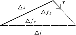
Figure 15: The geometry of the projection of an infinitesimal line segment taking into account kinematic effects. See text for details.

One configuration of the simple geometry relating the pre- and the post-projection length of an infinitesimal segment of the material line (at time $t$ around a position that is characterized by $u$) is illustrated in Fig. 15. The thick solid line in black is the pre-projection state of the infinitesimal line segment (of length $\Delta s$, where $s$ is the arc length along the material line and increases from the left to the right in Fig. 15), while the post-projection length is marked by a thick dashed line. The orientation of the former is determined by the dynamics and is given by the two components, $\Delta f_{x}$ and $\Delta f_{z}$, of the infinitesimal line segment corresponding to $\Delta s$, while the latter is horizontal. The post-projection length $\Delta l$ is determined by the direction of the velocity $\mathbf{v}$ as indicated by a thin dashed line in the figure (the velocity is assumed to be uniform in the infinitesimal domain considered here), and we are interested in the ratio of $\Delta l$ and $\Delta s$:

$$\mathcal{P}=\lim_{\Delta s\to 0}\frac{\Delta s}{\Delta l}.$$ (79)

As a vertical thin dashed line indicates in Fig. 15, the post-projection line segment can be divided to two sections, and $\Delta l$ can be calculated as the sum of the lengths of these two sections. The length of the left-hand-side section is simply $\Delta f_{x}$, while that of the right-hand-side one can be obtained as $\Delta f_{z}$ multiplied by the tangent of the angle enclosed by the two thin dashed lines. The latter is the opposite of the ratio of the two components of the velocity, so that we have $-\Delta f_{z}v_{x}/v_{z}$ for the length of the right-hand-side segment. Therefore, we have

$$\mathcal{P} =\lim_{\Delta s\to 0}\frac{\Delta s}{\Delta f_{x}-\Delta f_{z}\frac{v_{x}}{v_{z}}}$$

$$=\lim_{\Delta s\to 0}\frac{1}{\frac{\Delta f_{x}}{\Delta s}-\frac{\Delta f_{z}}{\Delta s}\frac{v_{x}}{v_{z}}}$$

$$=\left(\frac{\mathrm{d}f_{x}}{\mathrm{d}s}-\frac{\mathrm{d}f_{z}}{\mathrm{d}s}\frac{v_{x}}{v_{z}}\right)^{-1}$$ (80)

for the configuration presented if Fig. 15.

Other configurations (when $s$ increases from the right to the left or when the velocity has an essentially different direction) can be treated in a similar way, and the general result for the projection factor $\mathcal{P}$ differs from (80) only in an absolute value:

$$\mathcal{P}=\left|\frac{\mathrm{d}f_{x}}{\mathrm{d}s}-\frac{\mathrm{d}f_{z}}{\mathrm{d}s}\frac{v_{x}}{v_{z}}\right|^{-1}.$$ (81)

With the notation indicating that we are investigating an infinitesimal line segment of the material line at a time instant $t$ and that is characterized by the initial position $u$, we recognize (13).

Appendix J Stretching and projection for 3D flows

For $d=3$, let $\mathbf{f}(t=t_{0};\mathbf{u})$ be the parametric form of a planar sheet of initial conditions at time $t=t_{0}$, parameterized by the vector $\mathbf{u}=(u_{1},u_{2})$ that is an appropriate generalization of arc length (in the sense that $\int\int_{\mathbf{min}}^{\mathbf{max}}1\,\mathrm{d}^{2}\mathbf{u}$ gives the initial area of the sheet). Let $\sigma(t=t_{0};\mathbf{u})$ be the initial density within the sheet at $\mathbf{u}$. The density $\sigma_{\mathbf{x}}(t;\mathbf{u})$ at a point of the accumulation level whose initial preimage was characterized by $\mathbf{u}$ is given by

$$\sigma_{\parallel}(t;\mathbf{u})=\sigma(t=t_{0};\mathbf{u})\mathcal{F}(t;\mathbf{u})=\sigma(t=t_{0};\mathbf{u})\mathcal{S}(t;\mathbf{u})\mathcal{P}(t;\mathbf{u}),$$ (82)

where $\mathcal{F}(t;u)$ is the total factor multiplying the initial density,

$$\mathcal{S}(t;\mathbf{u})=\left|\frac{\partial\mathbf{f}(t;\mathbf{u})}{\partial u_{1}}\times\frac{\partial\mathbf{f}(t;\mathbf{u})}{\partial u_{2}}\right|^{-1},$$ (83)

with $\times$ denoting the vector cross product, is the factor representing stretching ($\mathbf{f}(t;\mathbf{u})$ stands for the image of the sheet at $t$), and

$$\mathcal{P}(t;\mathbf{u})=\left|\left(\frac{\partial\mathbf{f}(t;\mathbf{u})}{\partial s_{1}}-\frac{\mathbf{v}(\mathbf{f}(t;\mathbf{u}),t)}{v_{z}(\mathbf{f}(t;\mathbf{u}),t)}\frac{\partial f_{z}(t;\mathbf{u})}{\partial s_{1}}\right)\times\left(\frac{\partial\mathbf{f}(t;\mathbf{u})}{\partial s_{2}}-\frac{\mathbf{v}(\mathbf{f}(t;\mathbf{u}),t)}{v_{z}(\mathbf{f}(t;\mathbf{u}),t)}\frac{\partial f_{z}(t;\mathbf{u})}{\partial s_{2}}\right)\right|^{-1}$$ (84)

is the factor representing projection ($\mathbf{s}=(s_{1},s_{2})$ is the appropriate generalization of the arc length for the image of the sheet).

More direct forms are

$$\mathcal{F}(t;\mathbf{u}) =\left|\left(\frac{\partial\mathbf{f}(t;\mathbf{u})}{\partial u_{1}}-\frac{\mathbf{v}(\mathbf{f}(t;\mathbf{u}),t)}{v_{z}(\mathbf{f}(t;\mathbf{u}),t)}\frac{\partial f_{z}(t;\mathbf{u})}{\partial u_{1}}\right)\times\left(\frac{\partial\mathbf{f}(t;\mathbf{u})}{\partial u_{2}}-\frac{\mathbf{v}(\mathbf{f}(t;\mathbf{u}),t)}{v_{z}(\mathbf{f}(t;\mathbf{u}),t)}\frac{\partial f_{z}(t;\mathbf{u})}{\partial u_{2}}\right)\right|^{-1}$$ (85)

$$=\left|\left(\frac{\partial f_{x}(t;\mathbf{u})}{\partial u_{1}}-\frac{v_{x}(\mathbf{f}(t;\mathbf{u}),t)}{v_{z}(\mathbf{f}(t;\mathbf{u}),t)}\frac{\partial f_{z}(t;\mathbf{u})}{\partial u_{1}}\right)\cdot\left(\frac{\partial f_{y}(t;\mathbf{u})}{\partial u_{2}}-\frac{v_{y}(\mathbf{f}(t;\mathbf{u}),t)}{v_{z}(\mathbf{f}(t;\mathbf{u}),t)}\frac{\partial f_{z}(t;\mathbf{u})}{\partial u_{2}}\right)\right.$$

$$\left.-\left(\frac{\partial f_{y}(t;\mathbf{u})}{\partial u_{1}}-\frac{v_{y}(\mathbf{f}(t;\mathbf{u}),t)}{v_{z}(\mathbf{f}(t;\mathbf{u}),t)}\frac{\partial f_{z}(t;\mathbf{u})}{\partial u_{1}}\right)\cdot\left(\frac{\partial f_{x}(t;\mathbf{u})}{\partial u_{2}}-\frac{v_{x}(\mathbf{f}(t;\mathbf{u}),t)}{v_{z}(\mathbf{f}(t;\mathbf{u}),t)}\frac{\partial f_{z}(t;\mathbf{u})}{\partial u_{2}}\right)\right|^{-1}.$$ (86)

The second equation is due to the fact that the vectorial product in the first line has only one nonzero component. Unlike for $d=2$, the parametric derivatives of the position do not appear here in a simple combination. Nevertheless, (86) is equivalent to (6)-(8) for $d=3$. Formulae for $d>3$ can be constructed similarly.

Appendix K transforms the results to a matrix formulation, and links them to the local normal vector of the sheet at the time and place of its arrival to the accumulation level.

Appendix K The projection factor in 3D flows expressed in terms of the normal vector

Note that the right-hand side of (86) can be written as

$$\mathcal{F}(t;\mathbf{u})=\left|\det\left(J(t;\mathbf{u})\right)\right|^{-1},$$ (87)

where

$$J_{ij}(t;\mathbf{u})=\frac{\partial f_{i}(t;\mathbf{u})}{\partial u_{j}}-\frac{v_{i}(\mathbf{f}(t;\mathbf{u}),t)}{v_{z}(\mathbf{f}(t;\mathbf{u}),t)}\frac{\partial f_{z}(t;\mathbf{u})}{\partial u_{j}}$$ (88)

is a 2 by 2 matrix with $i,j\in\{x,y\}$. For $\det J$, the matrix determinant lemma Harville (2008) can be applied:

$$\det\left(J(t;\mathbf{u})\right)=\det\left(\frac{\partial\mathbf{f}_{\parallel}(t;\mathbf{u})}{\partial\mathbf{u}}\right)\left(1-\sum_{i,j\in\{x,y\}}\frac{\partial f_{z}(t;\mathbf{u})}{\partial u_{i}}\left.\frac{\partial u_{i}(t;\mathbf{f}_{\parallel})}{\partial f_{j}}\right|_{\mathbf{f}_{\parallel}=\mathbf{f}_{\parallel}(t;\mathbf{u})}\frac{v_{j}(\mathbf{f}(t;\mathbf{u}),t)}{v_{z}(\mathbf{f}(t;\mathbf{u}),t)}\right),$$ (89)

where $\mathbf{f}_{\parallel}(t;\mathbf{u})$ denotes the vector formed from the first two components of $\mathbf{f}(t;\mathbf{u})$, and $\mathbf{u}(t;\mathbf{f}_{\parallel})$ is the inverse of $\mathbf{f}_{\parallel}(t;\mathbf{u})$. The second factor in (89) can be simplified using the chain rule (note the sum for $i$), and one obtains

$$\det\left(J(t;\mathbf{u})\right)=\det\left(\frac{\partial\mathbf{f}_{\parallel}(t;\mathbf{u})}{\partial\mathbf{u}}\right)\left(1-\sum_{j\in\{x,y\}}\left.\frac{\partial f_{z}(t;\mathbf{u}(t;\mathbf{f}_{\parallel}))}{\partial f_{j}}\right|_{\mathbf{f}_{\parallel}=\mathbf{f}_{\parallel}(t;\mathbf{u})}\frac{v_{j}(\mathbf{f}(t;\mathbf{u}),t)}{v_{z}(\mathbf{f}(t;\mathbf{u}),t)}\right).$$ (90)

Now let us introduce the normal vector $\mathbf{n}$ of the surface $\mathbf{f}$:

$$\mathbf{n}(t;\mathbf{u}) =\left(\frac{\partial\mathbf{f}(t;\mathbf{u})}{\partial u_{1}}\times\frac{\partial\mathbf{f}(t;\mathbf{u})}{\partial u_{2}}\right)\left|\frac{\partial\mathbf{f}(t;\mathbf{u})}{\partial u_{1}}\times\frac{\partial\mathbf{f}(t;\mathbf{u})}{\partial u_{2}}\right|^{-1}$$

$$=\left(\frac{\partial\mathbf{f}(t;\mathbf{u})}{\partial u_{1}}\times\frac{\partial\mathbf{f}(t;\mathbf{u})}{\partial u_{2}}\right)\mathcal{S}(t;\mathbf{u}),$$ (91)

where the second line is obtained by substituting (83). Note that

$$n_{z}(t;\mathbf{u})=\det\left(\frac{\partial\mathbf{f}_{\parallel}(t;\mathbf{u})}{\partial\mathbf{u}}\right)\mathcal{S}(t;\mathbf{u}),$$ (92)

which can be substituted in (90). Furthermore, it can be shown that

$$n_{i}(t;\mathbf{u})=n_{z}(t;\mathbf{u})\left.\frac{\partial f_{z}(t;\mathbf{u}(t;\mathbf{f}_{\parallel}))}{\partial f_{i}}\right|_{\mathbf{f}_{\parallel}=\mathbf{f}_{\parallel}(t;\mathbf{u})}$$ (93)

for $i\in\{x,y\}$, so that (90) can be written as

$$\det\left(J(t;\mathbf{u})\right) =\mathcal{S}(t;\mathbf{u})^{-1}\left(n_{z}(t;\mathbf{u})+n_{x}(t;\mathbf{u})\frac{v_{x}(\mathbf{f}(t;\mathbf{u}),t)}{v_{z}(\mathbf{f}(t;\mathbf{u}),t)}+n_{y}(t;\mathbf{u})\frac{v_{y}(\mathbf{f}(t;\mathbf{u}),t)}{v_{z}(\mathbf{f}(t;\mathbf{u}),t)}\right)$$

$$=\mathcal{S}(t;\mathbf{u})^{-1}\frac{\mathbf{n}(t;\mathbf{u})\cdot\mathbf{v}(\mathbf{f}(t;\mathbf{u}),t)}{v_{z}(\mathbf{f}(t;\mathbf{u}),t)}.$$ (94)

According to (94) and (87), we finally have

$$\mathcal{F}(t;\mathbf{u})=\mathcal{S}(t;\mathbf{u})\left|\frac{v_{z}(\mathbf{f}(t;\mathbf{u}),t)}{\mathbf{n}(t;\mathbf{u})\cdot\mathbf{v}(\mathbf{f}(t;\mathbf{u}),t)}\right|,$$ (95)

from which

$$\mathcal{P}(t;\mathbf{u})=\left|\frac{v_{z}(\mathbf{f}(t;\mathbf{u}),t)}{\mathbf{n}(t;\mathbf{u})\cdot\mathbf{v}(\mathbf{f}(t;\mathbf{u}),t)}\right|$$ (96)

also follows.

One sees from (95) or (96) that the caustics (divergences in the denominator) are located where the local normal vector of the sheet is perpendicular to the local velocity, similarly to the $d=2$ case.

Appendix L Additional details about the dependence on the depth $a$ of several quantities in the double-shear flow

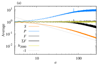
(a)

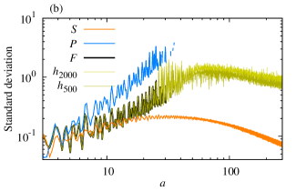
(b)

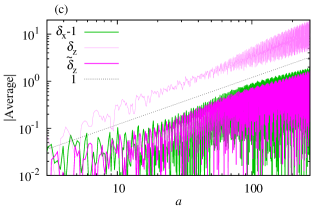
(c)

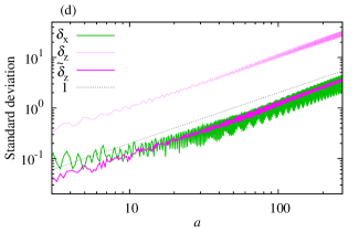
(d)

Figure 16: (a) The average and (b) the standard deviation, as a function of the accumulation depth $a$, of the same quantities as in Fig. 10. (c) The average and (d) the standard deviation of the parametric derivative of the horizontal position $\delta_{x}$ (minus $1$ for comparability), the parametric derivative of the vertical position $\delta_{z}$, and the weighted parametric derivative of the vertical position $\tilde{\delta}_{z}$. For comparison, the dashed lines mark power laws with the exponents indicated in the legend. $W=0.6$ and $A=0.07$.

Figure 16 exhibits an example when chaos is not observable. The average of each factor introduced in Section III.2, shown in Fig. 16a, starts with small slopes for small depths $a$. The average of the stretching factor, $\langle\mathcal{S}\rangle$, bends down for increasing $a$. In particular, for intermediate values of $a$, it might seem to follow a $1/a$ dependence. This would agree with the expectation that the reciprocal of the stretching factor, corresponding to the length of the line, should increase proportionally to time in this non-chaotic situation — but the line bends down even more for increasing $a$. The average projection factor, $\langle\mathcal{P}\rangle$, increases with depth, which is a natural consequence of the undulation of the material line. Approximately $\langle\mathcal{P}\rangle\approx 1/\langle\mathcal{S}\rangle$ until $a\approx 20$, and the increase of $\langle\mathcal{P}\rangle$ gets slower for larger values of $a$, which might be related to the bounded nature of the average effect of the projection. As a consequence of this behavior, the average total factor $\langle\mathcal{F}\rangle$ (still in Fig. 16a) is practically $1$ up to $a\approx 20$, and exhibits a slight decrease above (even though $\mathcal{F}=\mathcal{S}\mathcal{P}$ only pointwise, and $\langle\mathcal{F}\rangle\neq\langle\mathcal{S}\rangle\langle\mathcal{P}\rangle$). We are facing thus a net dilution for increasing depth, but without a known simple functional form. However, this dilution is local along the line: when summing up over the different branches of the line, the average $\langle\sum\mathcal{F}\rangle$ of the summed total factor does not follow the decrease in $\langle\mathcal{F}\rangle$. Instead, it remains remarkably close to a constant. The approximate conservation of $\langle\sum\mathcal{F}\rangle$ is not a surprise, since mass is conserved, and the horizontal support of the distribution of the particles changes very little in our example. The average $\langle h_{N}\rangle$ of the normalized histogram $h_{N}$, for $N=2000$ and also in a wide range in $N$ around this choice, is practically the same as $\langle\sum\mathcal{F}\rangle$ (without the spike near $a=80$, which indicates that probably this little spike is a numerical artifact).

The parametric derivatives, $\langle\delta_{x}\rangle$ and $\langle\delta_{z}\rangle$ (their absolute values are shown in Fig. 16c), obey a clear linear law as a function of $a$ (at least in terms of the envelope in the case of $\langle\delta_{x}\rangle$, which otherwise oscillates so strongly that sign changes occur in each “period” of the oscillation). This might be so because these quantities directly concern the final positions observed at the accumulation depth. Weighting $\delta_{z}$ by the local (time-dependent!) velocity does not ruin the linear functional relation, see $\langle\tilde{\delta}_{z}\rangle$ in Fig. 16c. The effect of this weighting is the reduction of the magnitude to approximately match that of $\langle\delta_{x}\rangle$ (without weighting, $\langle\delta_{z}\rangle$ is much larger, cf. Figs. 3c-5c and the related discussion), and the enhancement of the oscillations. The linear nature agrees with the regular dynamics, and with the proportional increase of the settling time for increasing depth $a$.

Turning to the characterization of the inhomogeneities, which we do by investigating the standard deviation of the relevant quantities, we can conclude from Fig. 16b that the total factor $\mathcal{F}$ (black line) exhibits an increasing inhomogeneity with increasing depth $a$ for approximately $a<30$, while there are no caustics, i.e., while it is meaningful to plot the line. The similarity in the functional form to that of that corresponding to the projection factor $\mathcal{P}$ (blue line) suggests the strong influence of this latter factor. The stretching factor is also getting more and more inhomogeneous at the beginning, but the increase in its standard deviation slows down, and turns to a homogeneization, which might be related to the decreasing magnitude of the factor $\mathcal{S}$ itself in average (as discussed in relation with Fig. 16a). As long as the standard deviation of the total factor $\mathcal{F}$ is meaningful, the standard deviation of the normalized histogram $h_{N}$ matches that of $\mathcal{F}$ very closely both for small ($N=2000$) and large ($N=500$) bin size, i.e., clearly indicates stronger and stronger inhomogeneities. However, later on, when the standard deviation of $h_{N}$ becomes $N$-dependent (at approximately $a=50$), inhomogeneization does not continue any more, but it turns to a homogeneization for any $N$, similarly to what is seen in the chaotic case (Fig. 10b).

The standard deviations of the parametric derivatives, as shown in Fig. 16d, increase in a simple, ballistic manner, in agreement with the regular features of the flow.

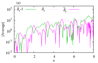
(a)

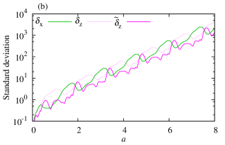
(b)

Figure 17: Same as Figs. 16c-16d for $A=0.25$.

In the chaotic case, illustrated by Figs. 10 and 17, the tendencies are always the same as in the regular case, the main difference lies in the functional forms of the dependences. The dependence of the averages and the standard deviations of the particular factors on $a$ are discussed in Section V.2 of the main text.

Fig. 17a indicates that the (unweighted and weighted) parametric derivatives exhibit a pronounced strengthening with $a$ in average, but the particular functional form is not clear. Note that, in contrast with the regular case of Fig. 16c, the unweighted parametric derivative $\delta_{z}$ of the vertical location is not larger in magnitude than the other two quantities in the plot (cf. Figs. 7c-8c). As for the standard deviations of the (unweighted and weighted) parametric derivatives, Fig. 17b shows that they do not increase with $a$ in a diffusional way (which could be expected in the presence of chaos), but follow an exponential law.

Summarizing the dependence on the accumulation depth $a$, we always experience a net local dilution with increasing depth, which is “neutralized” after summing up the different branches of the material line due to mass conservation. The inhomogeneities emerge at the beginning of the settling process (observable for small accumulation depths), and, if coarse-grained, they exhibit a decay on the long term (for large accumulation depths).

References

- Michaelides (1997) E. E. Michaelides, “Hydrodynamic Force and Heat/Mass Transfer From Particles, Bubbles, and Drops,” Journal of Fluids Engineering 125, 209–238 (1997).
- Falkovich and Fouxon (2002) G. Falkovich and M. G. Fouxon, I Stepanov, “Acceleration of rain initiation by cloud turbulence,” Nature 419, 151–154 (2002).
- Sabine et al. (2004) C. Sabine, R. Feely, N. Gruber, R. Key, K. Lee, J. Bullister, R. Wanninkhof, C. Wong, D. Wallace, B. Tilbrook, F. Millero, T. Peng, A. Kozyr, T. Ono, and A. Rios, “The oceanic sink for anthropogenic CO2,” Science 305, 367–371 (2004).
- Logan and Wilkinson (1990) B. E. Logan and D. B. Wilkinson, “Fractal geometry of marine snow and other biological aggregates,” Limnology and Oceanography 35 (1990), 10.4319/lo.1990.35.1.0130.
- Buesseler et al. (2007) K. O. Buesseler, A. N. Antia, M. Chen, S. W. Fowler, W. D. Gardner, O. Gustafsson, K. Harada, A. F. Michaels, M. Rutgers van der Loeff, M. Sarin, D. K. Steinberg, and T. Trull, “An assessment of the use of sediment traps for estimating upper ocean particle fluxes,” Journal of Marine Research 65, 345–416 (2007).
- Mitchell et al. (2008) J. Mitchell, Y. H., L. Seuront, F. Wolk, and H. Li, “Phytoplankton patch patterns: Seascape anatomy in a turbulent ocean,” Journal of Marine Systems 69, 247–253 (2008).
- Siegel and Deuser (1997) D. A. Siegel and W. G. Deuser, “Trajectories of sinking particles in the Sargasso Sea: modeling of statistical funnels above deep-ocean sediment traps,” Deep-Sea Research Part I-Oceanographic Research Papers 44, 1519 – 1541 (1997).
- Schlitzer, Usbeck, and Fischer (2003) R. Schlitzer, R. Usbeck, and G. Fischer, “Inverse modeling of particulate organic carbon fluxes in the south atlantic,” in The South Atlantic in the Late Quaternary: Reconstruction of Material Budgets and Current Systems, edited by G. Wefer, S. Mulitza, and V. Ratmeyer (Springer-Verlag Berlin Heidelberg New York Tokyo, 2003) pp. 1–19.
- Siegel, Fields, and Buesseler (2008) D. Siegel, E. Fields, and K. O. Buesseler, “A bottom-up view of the biological pump: Modeling source funnels above ocean sediment traps,” Deep-Sea Research I 55, 108–127 (2008).
- Qiu, Doglioli, and Carlotti (2014) Z. Qiu, A. Doglioli, and F. Carlotti, “Using a Lagrangian model to estimate source regions of particles in sediment traps,” Science China: Earth Sciences 57, 2447–2456 (2014).
- Monroy et al. (2017) P. Monroy, E. Hernández-García, V. Rossi, and C. López, “Modeling the dynamical sinking of biogenic particles in oceanic flow,” Nonlinear Processes in Geophysics 24, 293–305 (2017).
- Roullier et al. (2014) F. Roullier, L. Berline, L. Guidi, X. Durrieu De Madron, M. Picheral, A. Sciandra, S. Pesant, and L. Stemmann, “Particle size distribution and estimated carbon flux across the arabian sea oxygen minimum zone,” Biogeosciences 11, 4541–4557 (2014).
- Balkovsky, Falkovich, and Fouxon (2001) E. Balkovsky, G. Falkovich, and A. Fouxon, “Intermittent distribution of inertial particles in turbulent flows,” Phys. Rev. Lett. 86, 2790–2793 (2001).
- Bec (2003) J. Bec, “Fractal clustering of inertial particles in random flows,” Physics of Fluids 15, 81–84 (2003).
- Vilela et al. (2007) R. D. Vilela, T. Tél, A. P. S. de Moura, and C. Grebogi, “Signatures of fractal clustering of aerosols advected under gravity,” Phys. Rev. E 75, 065203(R) (2007).
- Cartwright et al. (2010) J. H. E. Cartwright, U. Feudel, G. Károlyi, A. de Moura, O. Piro, and T. Tél, “Dynamics of finite-size particles in chaotic fluid flows,” in Nonlinear Dynamics and Chaos: Advances and Perspectives, edited by M. Thiel, J. Kurths, M. C. Romano, G. Károlyi, and A. Moura (Springer Berlin Heidelberg, Berlin, Heidelberg, 2010) pp. 51–87.
- Guseva, Feudel, and Tél (2013) K. Guseva, U. Feudel, and T. Tél, “Influence of the history force on inertial particle advection: Gravitational effects and horizontal diffusion,” Phys. Rev. E 88, 042909 (2013).
- Guseva et al. (2016) K. Guseva, U. Feudel, A. Daitche, and T. Tél, “History effects in the sedimentation of light aerosols in turbulence: The case of marine snow,” Phys. Rev. Fluids 1, 074203 (2016).
- Ott (1993) E. Ott, Chaos in Dynamical Systems (Cambridge University Press, Cambridge, UK, 1993).
- Ottino (1989) J. M. Ottino, The Kinematics of Mixing: Stretching, Chaos and Transport (Cambridge University Press, Cambridge, 1989).
- Pierrehumbert and Yang (1993) R. T. Pierrehumbert and H. Yang, “Global chaotic mixing on isentropic surfaces,” J. Atmos. Sci. 50, 2462–2480 (1993).
- Gutknecht et al. (2013) E. Gutknecht, I. Dadou, B. Le Vu, G. Cambon, J. Sudre, V. Garçon, E. Machu, T. Rixen, A. Kock, A. Flohr, A. Paulmier, and G. Lavik, “Coupled physical/biogeochemical modeling including O2-dependent processes in the eastern boundary upwelling systems: application in the Benguela,” Biogeosciences 10, 3559–3591 (2013).
- Maxey and Riley (1983) M. R. Maxey and J. J. Riley, “Equation of motion for a small rigid sphere in a nonuniform flow,” Physics of Fluids 26, 883–889 (1983).
- Haller and Sapsis (2008) G. Haller and T. Sapsis, “Where do inertial particles go in fluid flows?” Physica D: Nonlinear Phenomena 237, 573–583 (2008).
- Jimenez (1997) J. Jimenez, “Ocean turbulence at milimiter scales,” Scientia Marina 61, 47–56 (1997).
- Wilkinson and Mehlig (2005) M. Wilkinson and B. Mehlig, “Caustics in turbulent aerosols,” EPL (Europhysics Letters) 71, 186 (2005).
- Drótos and Tél (2011) G. Drótos and T. Tél, “Chaotic saddles in a gravitational field: The case of inertial particles in finite domains,” Phys. Rev. E 83, 056203 (2011).
- Pierrehumbert (1994) R. Pierrehumbert, “Tracer microstructure in the large-eddy dominated regime,” Chaos, Solitons, and Fractals 4, 1091–1110 (1994).
- Feudel et al. (2005) F. Feudel, A. Witt, M. Gellert, J. Kurths, C. Grebogi, and M. Sanjuán, “Intersections of stable and unstable manifolds: the skeleton of lagrangian chaos,” Chaos, Solitons & Fractals 24, 947–956 (2005).
- Lindner and Donner (2017) M. Lindner and R. V. Donner, “Spatio-temporal organization of dynamics in a two-dimensional periodically driven vortex flow: A lagrangian flow network perspective,” Chaos 27, 035806 27, 035806 (2017).
- Bezuglyy et al. (2006) V. Bezuglyy, B. Mehlig, M. Wilkinson, K. Nakamura, and E. Arvedson, “Generalized Ornstein-Uhlenbeck processes,” Journal of Mathematical Physics 47, 073301 (2006).
- Gustavsson, Vajedi, and Mehlig (2014) K. Gustavsson, S. Vajedi, and B. Mehlig, “Clustering of particles falling in a turbulent flow,” Phys. Rev. Lett. 112, 214501 (2014).
- Lai and Tél (2011) Y.-C. Lai and T. Tél, Transient Chaos (Springer-Verlag, New York, 2011).
- Harville (2008) D. A. Harville, Matrix algebra from a statistician’s perspective (Springer-Verlag, New York, 2008).