Quantum-limited Parametric Amplification with Josephson Circuits in the Regime of Pump Depletion
Abstract
Linear parametric amplification is a key operation in information processing. Our interest here is quantum-limited parametric amplification, , amplification of quantum signals while adding the minimum amount of noise allowed by quantum mechanics, which is essential for any viable implementation of quantum information processing. We describe parametric amplifiers based on the dispersive nonlinearity of Josephson junctions driven with appropriate tones playing the role of pumps. We discuss two defining characteristics in the architecture of these amplifiers: the number of modes occupied by the signal, idler and pump waves and the number of independent ports through which these waves enter into the circuit. The scattering properties of these amplifiers is also reviewed. The main focus of this work are the computations of the dynamic range and phase-space distributions of the fluctuations of the modes of the amplifiers.
I Introduction
Photons of microwave radiation in the band (25-100 mm wavelength) have an energy approximately 105 smaller than those of visible light. Yet, at a temperature 2104 smaller than room temperature, now routinely achievable with commercial dilution refrigerators, it is possible to detect and process signals whose energy is equivalent to that of single microwave photons. Devoret and Schoelkopf (2013) There are three advantages of single photon microwave electronics when compared with quantum optics. First, signal envelopes with a relative bandwidth of a few percent at carrier frequencies of a few GHz can be controlled with much greater relative precision than their equivalent at few hundreds of THz. This is because microwave generators tend to have better short term stability than lasers, and also because microwave components are mechanically very stable, particularly when cooled, compared with traditional optical components. Second, on-chip circuitry of single-photon microwave electronics can be well in the lumped element regime and consequently, the control of spatial mode structure is more easily achieved than in the optical domain. Third, there exists a simple, robust, non-dissipative component, the Josephson tunnel junction, whose non-linearity can dominate over the linear characteristics of the circuit at the single photon level. Many quantum signal processing functions have thus been realized, both digital and analog. In this work, we concentrate on analog Josephson amplifying devices pumped with one or several microwave tones. In particular, only devices that demonstrate linear amplification with added noise at the level of the standard quantum limit Caves (1982) are considered here. These novel devices have taken the work pioneered by B. Yurke at the Bell labs thirty years ago Yurke et al. (1988, 1989) to the point where new original experiments can be performed successfully owing to Josephson amplifiers as the first link in the chain of measurements. Vijay et al. (2011); Hatridge et al. (2013)
The main desired characteristics of a Josephson amplifier are: i) low added noise: the noise added by the amplifier should be no larger than the minimum imposed by quantum mechanics, ii) high gain: the gain of the amplifier should be large enough (in practice, 20 dB or more) to beat the noise added by the subsequent stages in the amplifier chain, iii) large bandwidth: the amplifier should have a constant gain over a bandwidth that is large enough for the desired application, ranging from several MHz-s to several GHz-s, iv) large dynamic range: the amplifier should function as a linear device with output signal power proportional to the input signal power for a wide range of input signal power. This range of power, known as the dynamic range of the amplifier, should be large enough so that more than just a few incident photons can be reliably detected, v) unidirectional: the amplifier should, ideally, amplify only signals incident from the system being probed and deamplify signals coming from subsequent devices in the amplification chain. This is necessary to prevent spurious noise in other parts of the setup to propagate back into the system under measurement, vi) ease of operation: the necessary energy for the amplification process should be delivered to the amplifier in a manner that is as simple and robust as possible, without very precise tuning, vii) ease of construction: the circuit implementing the amplifier should have a minimal number of parts, and the parts should not require too delicate tolerances.
The aim of this article is to discuss the physics behind these Josephson parametric amplifiers in the high-gain regime where pump depletion effects can cause a reduction of the dynamic range of the amplifiers [item (iv) in the list above]. In particular, we provide a self-consistent, mean-field analysis of the dynamic range and stability of these amplifiers in this pump depletion regime. Furthermore, we analyze, in the same regime, the phase space distribution of the modes participating in the amplification process, building an understanding of the manner in which quantum fluctuations modify the parametric instability, the dark side of the phenomenon of amplification. This analysis is done within the framework of the Fokker-Planck equation. Although the focus of the paper is rather narrow compared to the above list of desired amplifier characteristics, for the sake of pedagogical clarity and to make the text self-contained, we review the fundamental amplifier characteristics like gain and bandwidth, which have been calculated elsewhere Kamal et al. (2009); Bergeal et al. (2010a); Abdo et al. (2013); Roy and Devoret (2016). We also compare several circuit realizations of these amplifiers, classified according to their number of modes and access ports.
The article is organized as follows. In Sec. II, the notion of effective parametric amplifier Hamiltonian is introduced. The important distinction between the degenerate and non-degenerate amplifiers that arises from a fundamental difference in the nature and number of degrees of freedom of the two kinds of devices is discussed. The linear scattering theory of these amplifiers is presented in this section. In practical amplifiers, the linear scattering theory ceases to be a sufficient description when the amplitude of the signal being amplified ceases to be infinitesimal compared to that of the pump tone giving rise to amplification. Then, the amplified output signal power is no longer a linear function of the input signal power. This more involved topic behind reduction of dynamic range, i.e. pump depletion effects leading to a reduction of gain of the device, is discussed in Sec. III. Phase-space fluctuations of the signals are calculated in Sec. IV. Several practical implementations of amplifiers are given in Sec. V. A concluding summary is provided in Sec. VII. For pedagogical reasons and to make the article self-sufficient, we have also included several appendices that familiarize the reader with the formalism required for theoretical analysis of the topics discussed in the main text. Appendix A extends the concept of classical signals to the quantum domain in the field of microwave electronics. Appendix B describes the important theoretical tool of the Quantum Langevin Equation (QLE) and input-output theory. Using this theory, the amplifier characteristics can be calculated, starting from the circuit Hamiltonian and the coupling parameters of its ports. We keep our treatments of the concepts in the appendices sufficient general and present them beyond the usual rotating wave approximation (RWA). Details of some of the calculations of the results presented in the main text are given in Appendices C and D.
II Model amplifiers
An amplifying circuit can be conveniently described as a collection of simple harmonic modes with time-dependent couplings. First, we address, using this model, the question of how a linear amplification function can arise from the Hamiltonian. Thus, let us consider the time-dependent effective quadratic Hamiltonian
| (1) |
where are bosonic mode annihilation operators and are circuit mode indices. The real, positive parameters and are, in general, functions of elementary parameters of the circuit combined with the values of time-dependent driving fields imposed from the outside and treated classically. We will see later in Sec. V how these effective parameters arise. The driving fields excite the circuit, thus providing energy for the amplification process and are often nicknamed “pumps”. Another important ingredient of the model is that there are ports that couple the modes to outside circuitry. In the case of one port per mode, this coupling is described by constants , the rate of excitation decay of mode through the port. The phase factors depend on the details of the excitation, while the drive frequencies are in the vicinity of (or sometimes ; this corresponds to photon conversion and we do not consider this case here). By vicinity, we mean within the bandwidth determined by the port coupling constants: . In this review, we will limit ourselves to two elementary cases: i) the two-port, two-mode, non-degenerate parametric amplifier with Hamiltonian:
| (2) |
and port coupling constants and , and ii) the one-port, one-mode, degenerate parametric amplifier with Hamiltonian:
| (3) |
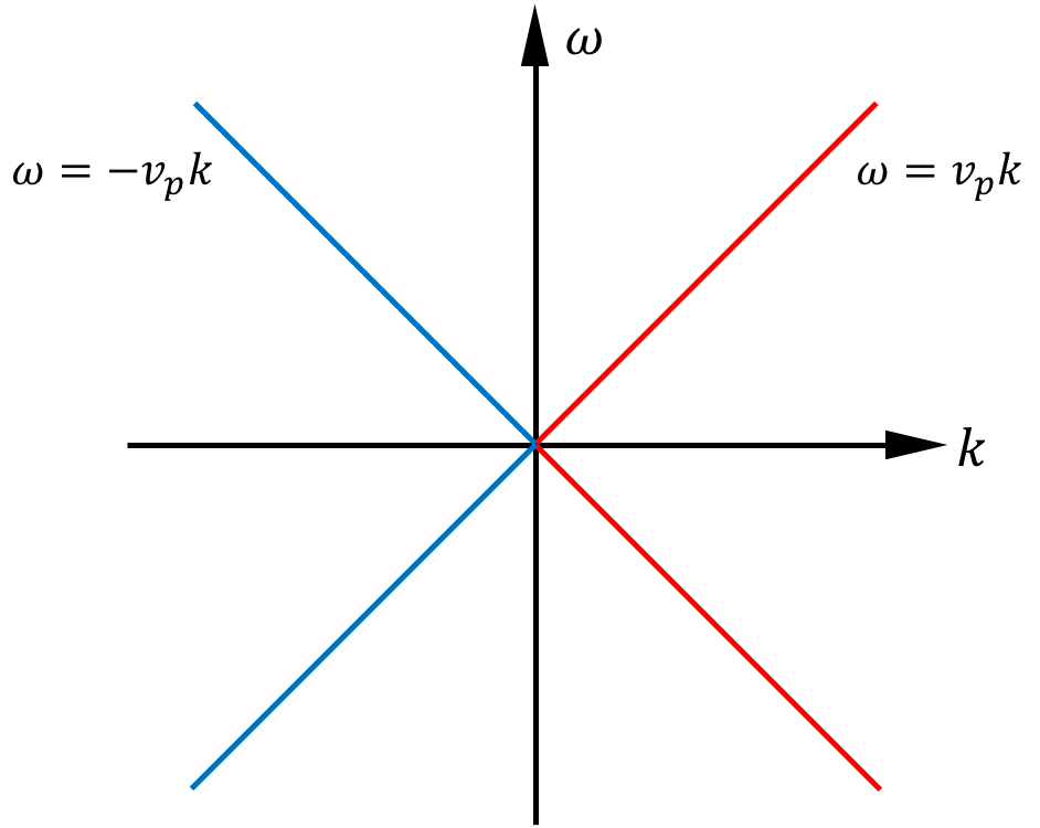
In this last case, there is a single port coupling constant . The frequency landscapes corresponding to the two cases are represented schematically on Fig. 1.

We deal with these model systems using the Quantum Langevin Equations (QLE-s), under rotating wave and Markov approximations (for derivation, see Appendix B). For the modes in the non-degenerate case, the QLE-s are given by:
| (4) |
where the input and output fields satisfy the boundary conditions:
| (5) |
Similarly, in the degenerate case, the QLE takes the form:
| (6) |
with the boundary condition:
| (7) |
From Eqs. (II), (5), we obtain for the non-degenerate case,
| (8) |
where . For the degenerate paramp, there is only one equation:
| (9) |
Going to the Fourier domain and solving for outgoing waves as a function of the incoming waves we find for the non-degenerate case:
| (10) |
where are the two signal and image (or idler) frequencies, respectively, linked precisely by . The operators at the negative frequencies should be interpreted as Hermitian conjugates of the same operators at the positive frequencies: (see Appendix A for details). Unlike in the case of simple harmonic circuits, an input signal at one frequency can here be processed into an output signal at another frequency. There is also a change in sign of the frequency in this process, which is called phase conjugation, and this is why we need to represent the scattering by a matrix. This matrix can be separated into two blocks related by complex conjugation relating Fourier coefficients with opposite frequencies, a mathematical operation independent of the physical phenomenon of phase conjugation. Phase conjugation manifests itself practically in the following manner: if one advances the phase of the input signal by a given quantity, the phase of the conjugated output signal becomes retarded by the same quantity. The elements of the scattering matrix are given by
| (11) | ||||
| (12) | ||||
| (13) | ||||
| (14) |
These expressions contain two ingredients: the single mode bare susceptibilities , which are given by
| (15) |
and the reduced effective mode coupling given by
| (16) |
Its modulus squared is often called the mode cooperativity. When the drive tone of the amplifier is optimally tuned at and the monochromatic input signals are on resonance with their corresponding mode , the scattering matrix takes the simpler form, with and . Here, the zero-detuning, optimal amplifier power gain is
| (17) |
It can be shown that the stability of the amplifier requires that , i.e. there is a ceiling to the effective coupling between modes of the circuit, beyond which amplification turns into spontaneous parametric oscillation. We will see later in Sec. III how this raw notion of stability ceiling is modified when the pump is treated more realistically.
Note that the determinant of the scattering matrix is unity even in the fully general case. Also, it is important to realize that, quite generally, the scattering is not reciprocal. A wave going from port b to port a acquires a phase factor from the drive which is conjugate to the phase factor accompanying the scattering from port a to port b.
We now turn to the degenerate case in which the scattering relations, involving only one port, still are expressed as a matrix:
Now, the different frequencies are carried on the same port and are all in the vicinity of the single resonance of the unique mode. Nevertheless, the scattering coefficients are similar to the previous expressions, with the substitution . A simplification occurs if the drive frequency is precisely tuned to twice the effective resonant frequency, i.e. , in which case and the subblock of the scattering matrix takes the form
| (24) |
with , and . Here, . We also introduce the in-phase and quadrature components of the incoming and outgoing waves:
| (25) |
where . The meaning of this transformation can be illustrated by the following consideration, which supposes for simplicity. Classically, if a signal is such that
| (26) |
with in-phase and quadrature modulation components and slow compared to , then
| (27) |
One can easily check that the effect of the angle associated with the time dependence of the effective Hamiltonian is just to rotate the component signals in the Fresnel plane. In the representation where the in-phase and quadrature components form the basis signals, we find that the scattering matrix is diagonal
| (28) | |||||
| (29) | |||||
The property of the scattering matrix to have unity determinant imposes
| (30) |
where . Thus, in this mode of operation of the degenerate parametric amplifier, one quadrature of the signal is amplified while the other is de-amplified. If the input signal consists only of vacuum fluctuations, the amplifier squeezes these fluctuations for one quadrature, making it less uncertain than the so-called standard quantum limit, which is associated to a standard deviation corresponding to the square root of a quarter of a photon (the half photon of the zero-point motion is split evenly between the two quadratures, and only one is squeezed). Walls and Milburn (2008); Drummond and Ficek (2013)
In the non-degenerate case (i) a more complex form of squeezing – two-mode squeezing – occurs in the four dimensional phase space of the quadratures of the two propagating signals incident on the circuit. Walls and Milburn (2008); Drummond and Ficek (2013) The non-degenerate parametric amplifier is usually employed as a sort of RF op-amp: the idler port is connected to a cold matched load emulating an infinite transmission line at zero-temperature and the device viewed from the signal port functions as a reflection amplifier operating in the phase preserving mode: for signals having a bandwidth small compared to that of the amplifier, we have
| (31) |
The second term on the right of this last expression shows that quantum noise entering through the b port must necessarily be added to the amplified signal. Caves (1982) This added noise contribution amounts, in the large gain limit and for an idler port at zero temperature, to a half-photon at the signal frequency, referred to the input. It can be seen as an evil necessary to preserve the commutation relation
| (32) |
More practically, the extra half-photon of noise can also be seen as a consequence of the Heisenberg Uncertainty Principle. A phase preserving amplifier processes equally both quadratures, which in quantum mechanics are non-commuting observables. Since the process of amplification is equivalent to measurement, the extra noise forbids that both quadratures are known precisely simultaneously, in accordance with the central principle of quantum mechanics. An amplifier functioning in this Heisenberg regime where the efficiency of the amplification process is only limited by irreducible quantum fluctuations is said to be quantum-limited.
III Dynamic range of amplifiers
In previous section, we have described the linear scattering theory of ideal amplifiers using effective, time-dependent, quadratic Hamiltonians. With such models, one can, in principle, achieve arbitrary high gains in amplifiers. However, in realistic situations, there are two major effects that reduce of the gain of the amplifiers, as described below.
First, the nonlinearity giving rise to the desired mode-mixing rarely ever yields only the desired quadratic Hamiltonian. In practice, higher order terms such as quartic (Kerr) terms cannot be neglected even if their amplitude is smaller than the main quadratic terms. In the presence of pump and incident signals, these relatively small quartic terms are sufficient to shift the resonator frequencies appreciably (this effect is also known as the AC-Stark shift). This results in the incident pump of Eqs. (2, 3) being off-resonant, and thus, the gain of these devices is lowered [see Eqs. (11-14)]. Recent results (see Ref. Liu et al., 2017) indicate that this is the dominant source of gain saturation in current parametric amplifiers. More details on how this arises is given in the discussion of implementation of parametric amplifiers [see Sec. V.1, in particular Eqs. (80-82)]. We note that recently, a method to implement three-wave mixing while suppressing the detrimental effects of the fourth order nonlinearity has been proposed. Zorin (2016); Frattini et al. (2017)
Second, pump depletion, which occurs due to the large magnitude of the signal being amplified, also limits the gains of amplifiers. When the amplitude of the incident signal being amplified is infinitesimal compared to that of the pump, the number of photons required from the pump for amplification is negligible compared to the total number of photons present in it. Thus, the pump tone can be considered to be stiff and its amplitude and phase can be treated as parameters without dynamics. This is the case in Sec. II. However, as the amplitude of the signal grows, the number of photons required for amplification also grows. As a result, the pump tone gets depleted, which leads to a reduction of the gain of the device. Note that even in absence of any incident signal, vacuum fluctuations are always incident on all the ports, which forbid, in a precise analysis, to consider the pump as perfectly stiff. This is because amplification of these vacuum fluctuations also leads to a reduction of the dynamic range of the device.
In this section, we calculate the gain saturation of our model amplifiers. In our analysis, we only consider pump depletion due to the finite size of the incident signal. We model the pump as a classical drive incident on a low-Q mode coupled to the modes being amplified. We calculate the resultant gain and the output signal power in a self-consistent manner. In effect, we perform a mean-field calculation for the incident pump tone, neglecting its quantum fluctuations. For simplicity, we consider the situation when the pump tones meet the resonance condition for amplification and neglect incident thermal photons on all the ports 111For similar analysis in a related topic, see Refs. Lähteenmäki et al., 2013, 2016..
Thus, we start with the following Hamiltonian for the non-degenerate parametric amplifier:
| (33) |
where where respectively denote the signal, idler and pump modes for the device 222Such a trilinear Hamiltonian arises also in treatment of Hawking radiation from a quantized source Nation and Blencowe (2010). (see Sec. V.4 for a practical implementation). The QLE-s for the modes are given by
| (34) | ||||
| (35) | ||||
| (36) |
Here , , denote the frequencies and , , the decay-rates for the modes . Furthermore, denote the nonlinear coupling between them. We require the Q-factor of mode to be much lower than that of : . The annihilation operators for the signal, idler and the pump are given by and . The incident pump tone is in a coherent state with amplitude (phase) , on resonance with the cavity frequency . In practice, the pump tone is often delivered through a rather high-Q, but off-resonance resonator which ends up being populated with very few photons. This type of impedance mismatch while closer to reality, involves more elements to be described correctly, and we have simplified it without losing the end results. In any case, , where is the number of photons in steady-state in the -mode. Under the stiff pump approximation, the term in Eq. (41) is neglected. Thus, the mode is in a coherent state, with its amplitude, in steady state, given by
| (37) |
Replacing in Eqs. (34, 35) results in the linearized dynamical equations for , given earlier in Eq. (II), with
| (38) |
For the degenerate case, the corresponding Hamiltonian is given by:
| (39) |
where respectively denote the signal and pump modes for the device (for its practical implementation, see Sec. V.3). The QLE for the modes are given by
| (40) | ||||
| (41) |
The stiff pump approximation, in this case, leads to a linear QLE for , giving rise to the scattering matrix in Eq. (24) in Sec. II. The parameters of the scattering matrix relate to the pump tone parameters as follows:
| (42) |
In order to incorporate the effect of pump depletion for the non-degenerate (degenerate) case, one needs to include the previously neglected term in the analysis and solve for self-consistently. Since we are interested in parameter regimes where the pump depletion is small, yet non-negligible, we will treat the pump mode as a coherent state and perform a perturbation analysis around the un-depleted value for :
| (43) |
and solve for self-consistently. The equation of motion for , for the non-degenerate and degenerate cases, are respectively given by
| (44) |
and
| (45) |
Consider the non-degenerate case. In the Fourier domain, Eq. (44) can be written as
where in the last line, we have used the input-output relations Eq. (5). We treat the case when there is an incident tone on the -mode with a photon flux per unit time (see Eq. (167) for definition). Our results can be generalized easily to the more complicated case of both and modes being driven. Substituting the expression of , from Eq. (10), after several lines of algebra, we arrive at
where we have neglected the number of thermal photons present in the transmission lines. Fourier transforming back, we get
Using the above expression for , we arrive at the self-consistency relation for :
where the second and third terms on the right denote the pump depletion due to incident signal and vacuum fluctuations on the signal port. Here, . Using the above equation, one can compute the gain and the output signal power (see Appendix C) given by
| (46) | ||||
| (47) |
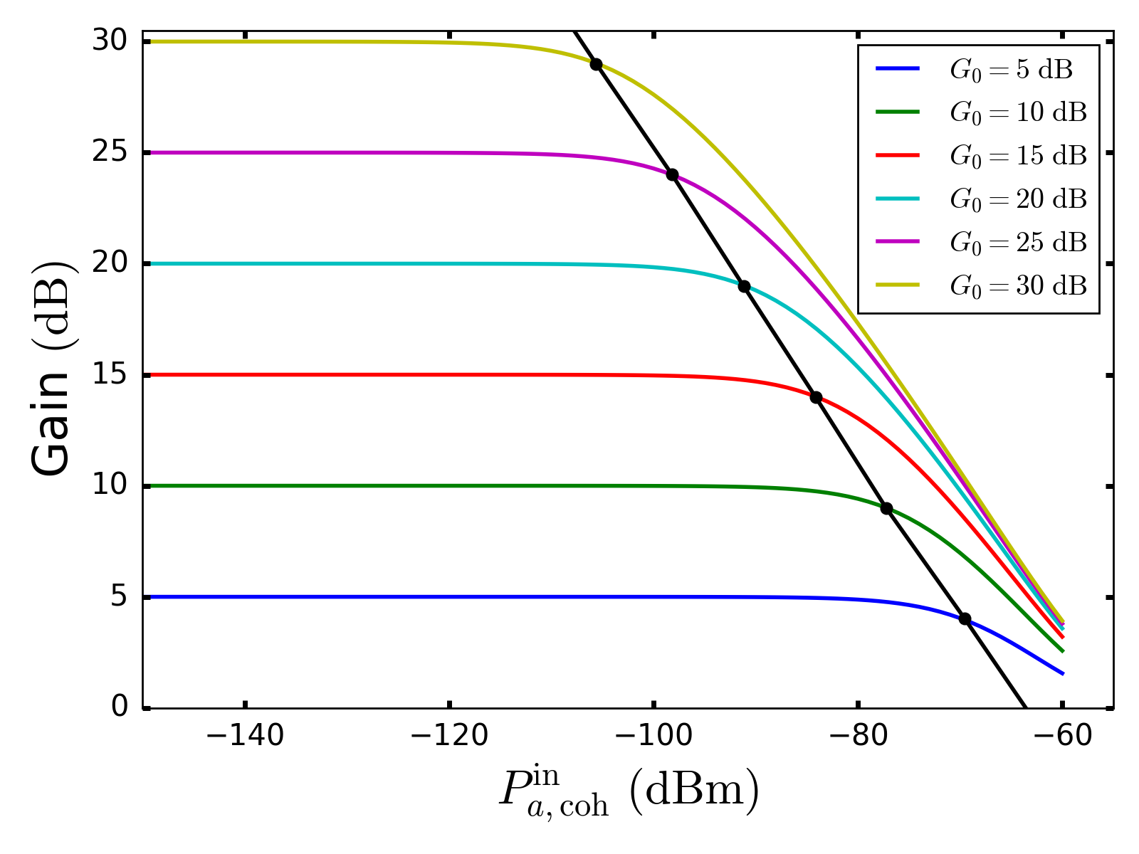
Fig. 2 shows the resulting gain as a function of coherent incident signal power () for the non-degenerate case. The different curves correspond to un-depleted gain of to dB, in steps of dB. The black dots on each curve correspond to the point where the gain of the amplifier is lowered by 1 dB. These points lie on a straight line, with a slope of . This is in reasonable agreement with the asymptotic value of the slope in the limit of high gain, predicted to be [see Eq. (103) in Ref. Abdo et al., 2013].
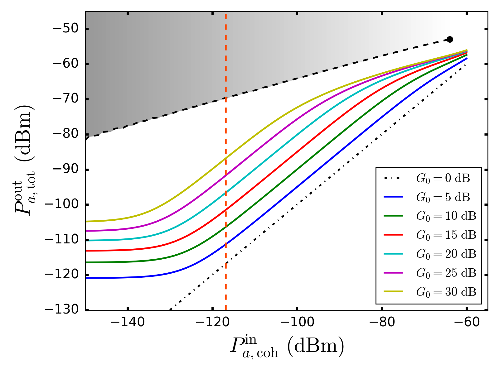
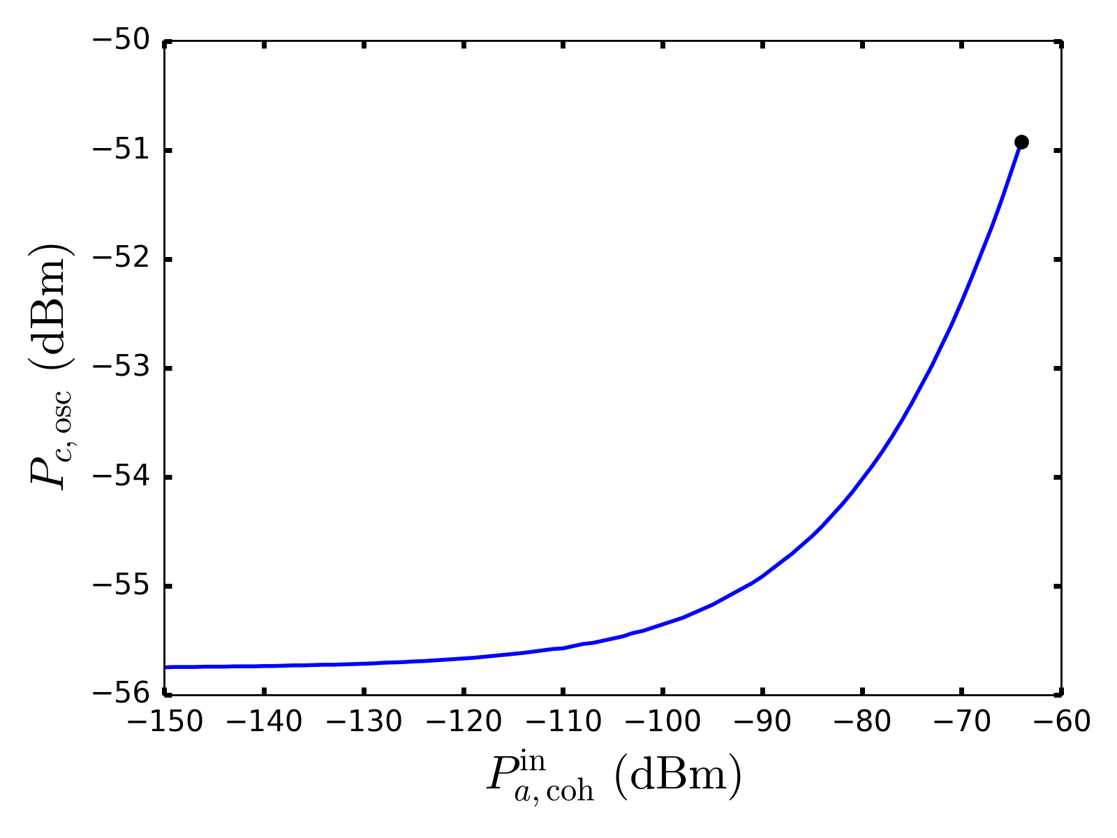
In Fig. 3, the total output signal power is plotted as a function of . The solid curves denote the output power for un-depleted gain of to dB, in steps of dB. As the incident coherent signal power goes to zero, the output power tends to a constant value which corresponds to amplified vacuum fluctuations incident on the signal port. The black dot-dashed line correspond to unity un-depleted gain when the pump tone is switched off. Finally, the dashed black line correspond the maximum output power that the device can produce before the onset of spontaneous parametric oscillation333This curve can be obtained as follows. Solving the coupled nonlinear set of equations [Eqs. (34, 35, 36)] in steady state, one obtains the smallest pump power which gives rise to multiple, stable, steady-state solutions for the modes . The pump power immediately below this value is the maximum allowed pump power. In practice, the equations are solved numerically for different pump powers. . For low enough incident power, the dashed line eventually approaches a constant value like the solid curves. This regime falls outside the range of incident powers shown in the plot. The shaded region above the dashed line indicates the region where the system shows spontaneous oscillation. In this region, the noise spectrum of the amplifier output develops a peak at the self-oscillation frequency, which rides on top of a continuous background. Note that as the incident signal power is increased, the pump power needed for onset of oscillation, the threshold pump power, increases (see Fig. 4). For sufficiently high incident signal power, the system ceases to exhibit parametric oscillation (denoted by the black circle in Figs. (3, 4). We note that the solid curves asymptotically do not approach the dashed line of the onset of parametric oscillation (there is a gap of about 5 dB). The reason for that is as follows. The self-consistent theory for the solid curves [Eqs. (46, 47] is derived using the linear scattering relations of the parametric amplifier [see Eq. (10)]. Thus, onset of parametric oscillation, which is inherently a nonlinear effect, is beyond the scope of this theory. We believe a more complete theory of pump depletion will be able to address this discrepancy. The details of such a theory is left for a future work.
The aforementioned parametric oscillation in these parametric amplifiers is analogous to the second order phase-transition occurring in ferromagnets. For the non-degenerate case, consider a two-dimensional ferromagnet (which has a complex scalar magnetization order parameter) in four or higher dimensions. Here, the dimension is chosen to make the analogy with our mean-field calculations more appropriate. For simplicity, we choose the pump phase appropriately so that Eqs. (34-36) allow for solutions for , where are real. In this analogy, the role of the complex magnetization order parameter is played by . The role of the inverse temperature is played by the incident pump tone amplitude . The incident signal acts like an external applied magnetic field. In this analogy, the black dashed line corresponds to a second-order phase-transition, terminating at a critical point. However, note the qualitative difference to conventional phase-transitions in this analogy. In ferromagnets, in presence of magnetic field, the second order phase-transition disappears in favor of a smooth crossover. In the non-degenerate amplifier, the parametric oscillation persists for a range of the incident signal.
The calculations for the degenerate case proceeds analogously and leads to
Here, we have neglected the generated second order harmonic. This harmonic does not contribute to amplification within the RWA. Using the above expression for , we arrive at the self-consistency relation for :
where . The gain and the output power on the signal port are respectively given by
| (48) | ||||
| (49) |
The plots for the degenerate case are shown in Appendix D. Analogies with phase-transitions in ferromagnets can also be constructed for the degenerate case and is omitted for brevity.
IV Phase-space distribution of parametric amplifiers: below, at and above threshold
Whereas in the previous sections, we have analyzed degenerate and non-degenerate parametric amplifiers in the Heisenberg picture, here in this section, we turn to the Schrödinger picture and the associated Lindblad master equation to analyze the phase-space distributions of the modes. This approach has the merit of directly yielding the variance of the fluctuations of the signal and idler waves. Starting from the Lindblad equation, we derive an effective Fokker-Planck equation for the Wigner distribution for the relevant modes. These are subsequently solved analytically to get the results. Our calculations extend those given in Chap. 10 of Ref. Carmichael, 2007. Here, we begin with the case of a degenerate paramp since it is computationally easier.
IV.1 Degenerate parametric amplifier
The Lindblad equation for the density matrix for the modes of a degenerate paramp is given by
| (50) |
where is defined in Eq. (39),
| (51) |
and is the Lindblad superoperator. Here denote the incident signal (pump) tone. Using the definition of the Wigner distribution in terms of the symmetrized characteristic function (see Chap. 10 of Ref. Carmichael, 2007 and Chap. 4 of Ref. Carmichael, 1999), one can write down the equation of motion for , where denote the complex numbers corresponding to amplitudes of the modes respectively. The resulting equation is given by
| (52) |
While the above equation describes the full dynamics of the Wigner distribution, it is not amenable to analytical solution. To achieve the latter, we expand the mode amplitudes around the semi-classical solutions and look at small fluctuations around these solutions. For the degenerate case, this approach is valid for all values of pump and signal power (see below for the non-degenerate case). For nonzero incident signal power (), the fluctuations of the modes are small compared to their semiclassical values by a factor of (the proof is identical to that presented in Chap. 10 of Ref. Carmichael, 2007 and Chap. 8 of Ref. Carmichael, 1999). Here is the number of pump (-mode) photons required to give rise to spontaneous oscillation of the mode for . The formula for is
| (53) |
which is obtained by setting of Sec. III to 1. This scaling of the fluctuations is a manifestation of the fluctuations of the modes remaining Gaussian for all values of the pump power (see Fig. 5 below, bottom panels). However, the situation is different for zero incident signal power () at the threshold of spontaneous oscillation. For , at the threshold, the fluctuations are damped by a factor of (see Chap. 10 of Ref. Carmichael, 2007 for proof). This is a manifestation of the non-Gaussian behavior of the fluctuations of the signal mode (see Fig. 5 below, top center panel). In the following, we perform the calculations for . Since the details for are given in Chap. 10 of Ref. Carmichael, 2007, we do not repeat that calculation here. We define
| (54) |
where , , , and , . Here, denote the fluctuations around a semi-classical solutions . Performing the analysis self-consistently and omitting some algebra, we arrive at the equations of motion for the semi-classical solutions:
| (55) | ||||
| (56) |
where . Note that these equations are merely scaled, semi-classical versions of the QLE-s derived in Sec. III. The fluctuation around these semi-classical solutions is given by the Wigner distribution , which obeys
| (57) |
This equation for is a Fokker-Planck equation and thus, can be exactly solved as a function of time. Therefore, any correlation function of the modes can also be analytically computed using this equation. Next, we give the steady state properties of when . Computations for other choices of can be performed analogously. In steady state,
| (58) |
where , and individually obey the following Fokker-Planck equations:
| (59) |
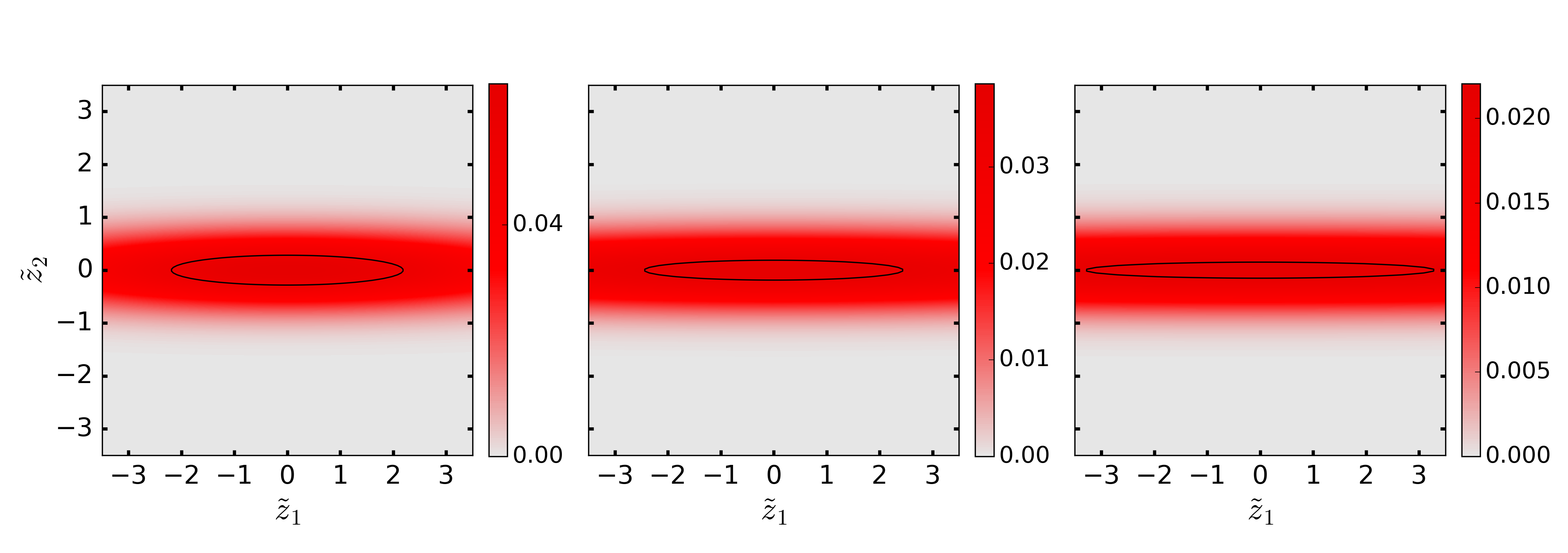
Here, denote the semi-classical solutions obtained by solving Eqs. (55, 56) in steady state. For nonzero , the fluctuations around the semi-classical solutions remain Gaussian for all values of the pump , even though the system shows parametric oscillation (see Sec. III) for a range of . This should be compared to the case when . In that case, below and above the threshold for spontaneous oscillation, the fluctuations around the semi-classical solution are Gaussian, while the system exhibits non-Gaussian behavior at threshold. The results of the calculations are shown in Fig. 5. The top panels show the case when . The top left and top right panel shows the fluctuations of the -mode around semi-classical solution below and above the spontaneous oscillation threshold. The top center panel shows the non-Gaussian behavior of the system at the threshold in absence of incident signal, as indicated by the contour lines which are no longer ellipses. The bottom panels show the Wigner function of the signal mode when for the corresponding pump powers.
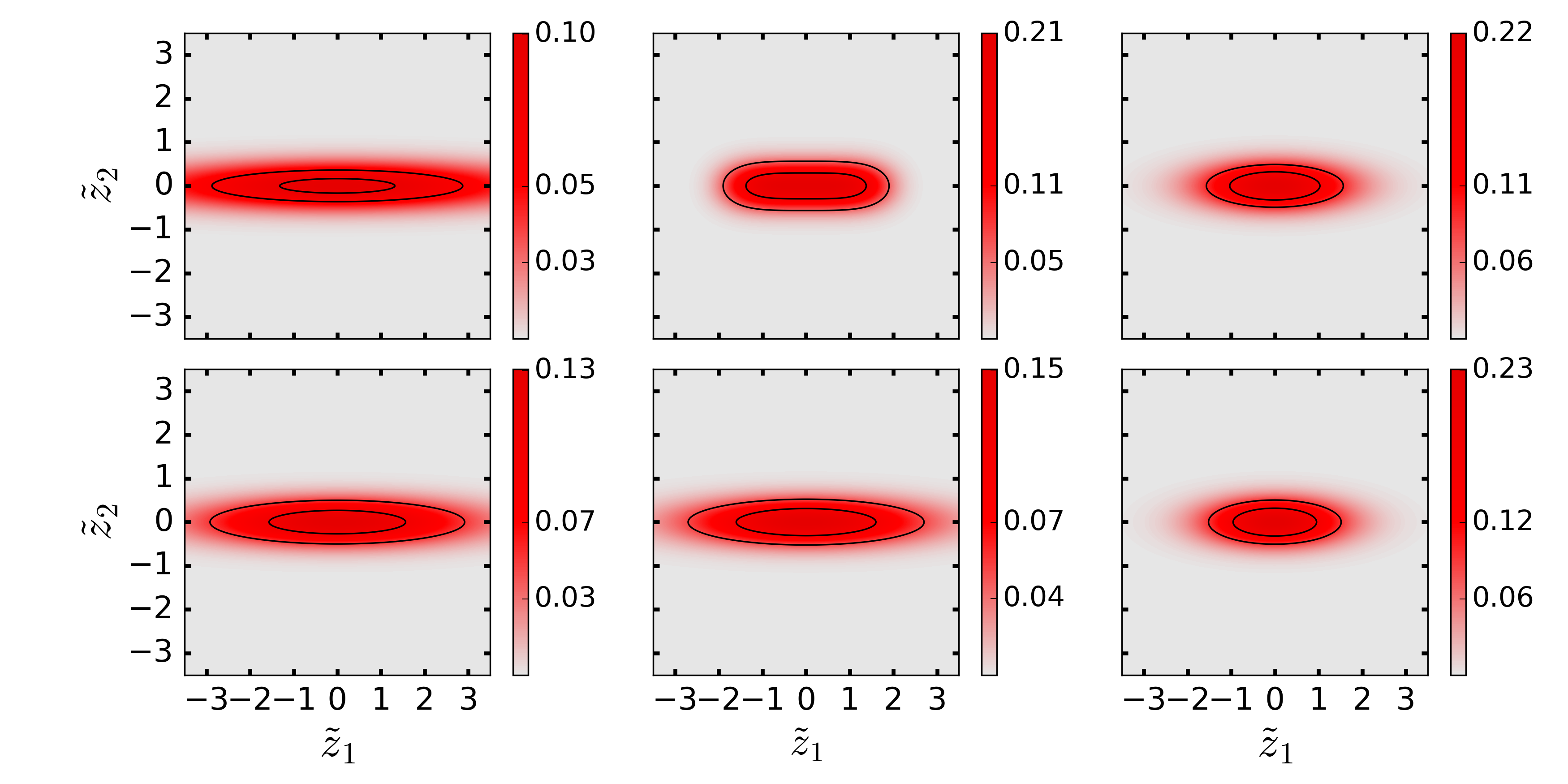
Note that for , the output amplified signal exhibits correlations with the pump tone. This is evident from the factorization of the Wigner function [see Eq. (58)], where one quadrature of the signal is correlated with one of the pump. As the amplitude of the incoming signal becomes smaller, this correlation decreases and vanishes completely only in the limit .
IV.2 Non-degenerate parametric amplifier
Next, we describe the phase-space distribution of the modes of a non-degenerate parametric amplifier when there is an incident signal on the -mode. The case when both and modes are driven can be treated analogously. The equation of motion for the system is given by
| (60) |
where is defined in Eq. (33) and
| (61) |
As in Sec. III, we consider the case when only the signal mode is driven, with denoting the incident signal (pump) tone. Then, the equation of motion for the Wigner distribution is
| (62) |
For non-zero incident signal power (), the analysis is analogous to the degenerate case. The fluctuations around the semiclassical amplitudes remain Gaussian for all values of pump powers. They are smaller than the classical amplitudes by the factor of , where now
| (63) |
This is obtained by setting of Sec. III to 1. In absence of incident signal, below and at the threshold of oscillation, the fluctuations of the modes are respectively Gaussian and non-Gaussian and the scaling is identical as in the degenerate case. However, above threshold there is a qualitative difference between the degenerate and non-degenerate cases. Unlike the degenerate case, the phases of self-oscillating amplitude of the modes are undetermined above threshold in absence of an incident signal. This, together with the decay of the modes , gives rise to phase-diffusion. A full treatment of this effect needs the use of the positive-P distribution (see Ref. Reid and Drummond, 1989 for more details) and goes beyond the scope of this article. Here, we will only treat the case when there is an incident signal which is relevant for amplifiers. Then, the Wigner distribution is sufficient to analyze the system. We define
| (64) |
Here, , , , , , and , , . The variables denote the fluctuations around the semi-classical solutions . Expanding self-consistently, one arrives at the semi-classical equations of motion:
| (65) | ||||
| (66) | ||||
| (67) |
where . Once again, these are merely the scaled, semi-classical versions of the QLE-s derived in Sec. III. The fluctuations are determined by the Wigner distribution , which obeys the following:
| (68) |
For simplicity, we choose and the phases of so that the semi-classical solutions are real. In steady state, the above Fokker-Planck equation factorizes and , where obeys
| (69) |
and and denote the steady state solutions of Eqs. (65-67). The above equations can be solved analytically. The cut of the Wigner distribution showing the phase-space fluctuations of the signal mode is given in Fig. 6. Due to the presence of the incident signal, the fluctuations are always Gaussian (as in the degenerate case). The three panels correspond to pump powers that, in absence of incident signal, correspond to below, at and above threshold of spontaneous oscillation. Note that the incident signal also removes the phase-diffusion present in the non-degenerate parametric oscillator above threshold Reid and Drummond (1989) (see right panel). The modes are correlated with the pump mode for finite [this can be also seen from the factorization of the Wigner function in Eq. (IV.2)]. This correlation is exactly zero only for . Of course, in this case of two-mode squeezing, the modes stay correlated for all values of .
V Practical amplifier circuits based on Josephson junction circuits
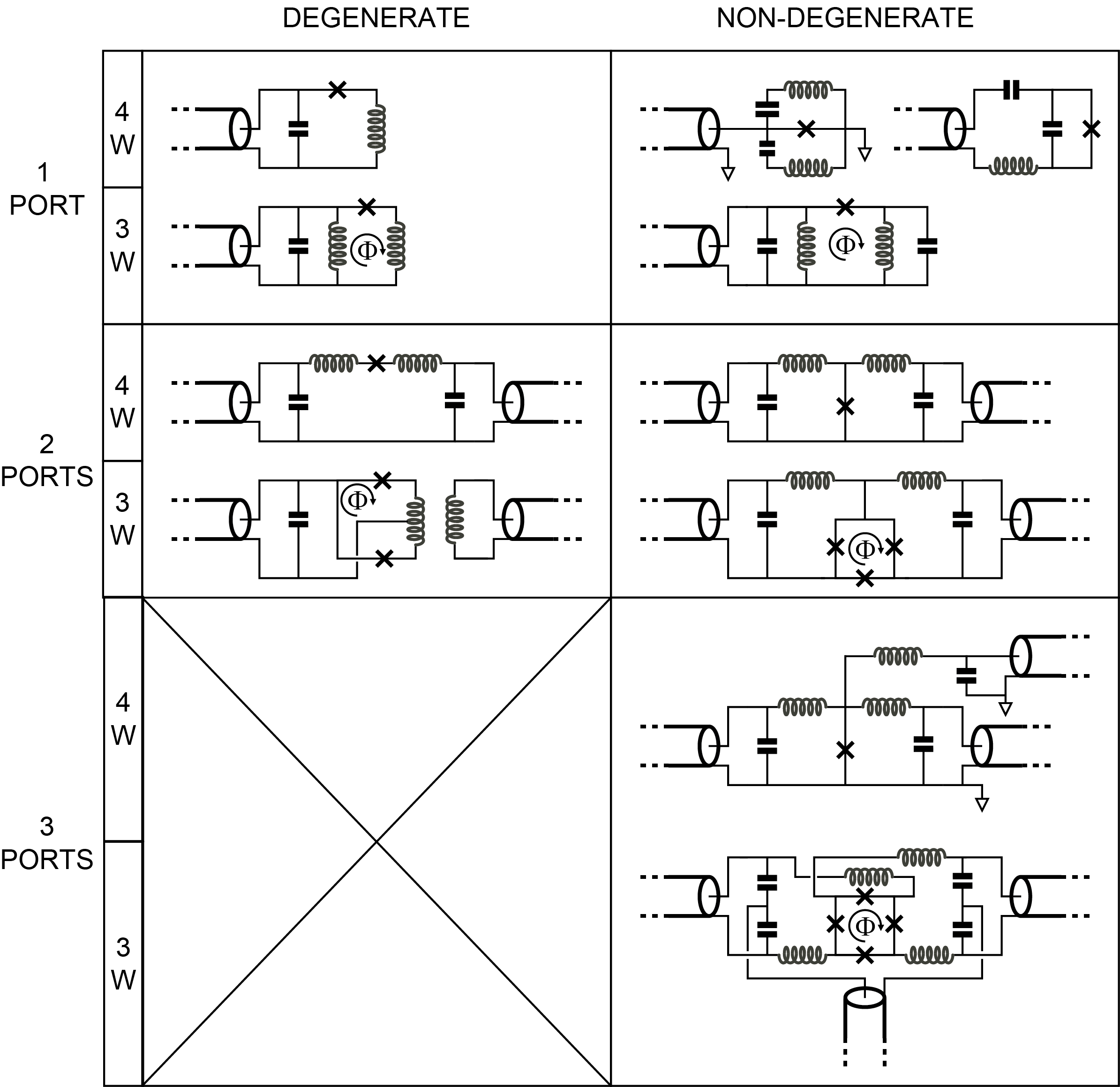
In this section, we provide several circuit realizations of the degenerate amplifiers (Secs. V.1, V.2, V.3) and a non-degenerate amplifier (Sec. V.4). The circuit construction, together with pros and cons of each approach, is discussed. A concise summary of the different circuit constructions is provided in Fig. 11.
V.1 Driven microwave oscillator whose inductance is a single Josephson element: Duffing-like dynamics
We first examine the simplest case of a one-mode, one-port circuit in which the inductance is just the Josephson element of superconducting tunnel junction (see Fig. 7) Siddiqi et al. (2004); Vijayaraghavan (2008).
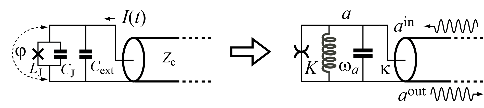
The Hamiltonian of such systems is given by
| (70) | |||||
| (71) |
where is the Josephson energy, is the total capacitance in parallel with the Josephson element, the gauge-invariant phase difference across the junction, the charge conjugate to the phase , the Hamiltonian of the transmission line, including the pump arriving through this channel and the current operator belonging to the degrees of freedom of the line. The amplifier functions with having excursions much less than and the cosine function in the Hamiltonian can be expanded to order only, with the term treated as a perturbation Manucharyan et al. (2007); Nigg et al. (2012). Introducing the ladder operators of the single mode of the circuit
| (72) |
and working in the framework of both an expansion in and RWA, the hamiltonian of the circuit simplifies to
| (73) |
where, in the regime , and . The QLE applied to this system yields
| (74) |
where . This last equation is the quantum version, in the RWA approximation, of the equation describing systems modeled by the Duffing equation. The classical Duffing oscillator obeys the equation
| (75) |
for the position variable having mass , small amplitude spring constant , friction coefficient and driven at frequency , which is close to the small amplitude resonant frequency . A small probe force allows to study the displacement response of the system. Non-linearity of the oscillator corresponds here to the spring constant being dependent quadratically on position.
Here, for our amplifier, plays the role of the damping rate , and plays the role of . Let us now suppose that, in addition to the signal to be processed, the port also receives an intense drive tone described by a propagating coherent state with amplitude and frequency . We treat this drive by the change of variable
| (76) | |||||
| (77) |
We aim to solve for the semi-classical amplitude from Eq. (74):
| (78) |
By treating the non-linear term as a perturbation, we obtain the self-consistent algebraic equation in steady state:
| (79) |
which in general yields for the c-number a complex value . Here,
| (80) |
Expanding around this value [using Eq. (77)] and keeping up to second order terms, we arrive at the effective Hamiltonian for the degenerate parametric amplifier arising from the pumping of the Josephson junction
| (81) |
with
| (82) |
The analysis of the amplifier based on the Hamiltonian given by Eq. (81) is justified only for small compared to other spurious couplings/measurement times. Note that Eq. (82) puts into light two drawbacks of this type of amplifier: the center frequency of the band of the amplifier shifts as the pump amplitude is increased and the pump tone needs to be at the center of the band for optimal amplification. The use of two pumps frequencies and such that facilitates the use of this parametric amplifier. Kamal et al. (2009)
The device has noticeable gain when is of order unity, implying that the number of pump photons in the oscillator is of order , a large number by hypothesis. This justifies our treatment of the pump drive as a c-number. Neglected terms such as the non-RWA term have smaller factors and can themselves be treated as perturbations on top of the standard degenerate parametric amplifier formalism. It is worth noting that for this device, the pump tone and the signal tone must enter the circuit on the same port, which is inconvenient given the widely different amplitude levels of these two waves.
V.2 A parametrically driven oscillator: the DC-SQUID driven by RF flux variation
Another class of Josephson circuit implementing parametric amplifiers at microwave frequencies is the RF-Flux-driven DC-SQUID (see Fig. 8).
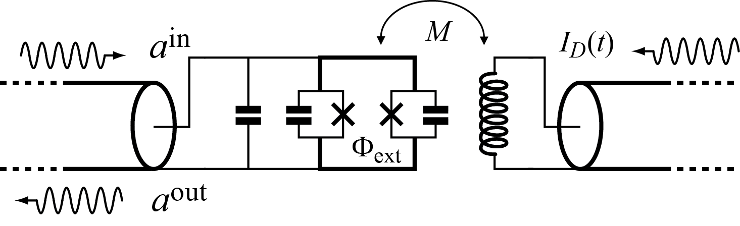
It turns out that this parametric drive can be implemented in Josephson circuits by taking a DC-SQUID, which is formed by two nominally identical Josephson junctions in parallel and modulating at the RF pump frequency the flux threading the superconducting loop between them (here the term DC refers to the circulating current in the loop due to an external bias flux). One exploits the functional form of the Josephson inductance of the DC-SQUID
| (83) |
where is the flux quantum and is the Josephson inductance of each individual junction. When
| (84) |
with close to the resonant frequency of the SQUID and , one implements the parametrically driven harmonic oscillator with relative frequency modulation parameter . This modulation is produced by a drive current at the primary of the transformer coupling the transmission line of an RF pump to the flux of the SQUID (see Fig. 8). Classically, the parametrically driven harmonic oscillator obeys the equation
| (85) |
In contrast with the Duffing oscillator above, this system is described by a fully linear, albeit time-dependent, equation. The drive, instead of appearing as a force coupled directly to position, now modulates the spring constant with a relative amplitude . The system behaves as an amplifier when the argument of the cosine modulation term is such that the drive frequency is close to the resonant frequency . In the weak damping limit , the quantum version of this oscillator is directly a one-port, one-mode system described by our degenerate amplifier Hamiltonian
| (86) |
where
| (87) | |||||
| (88) |
Note that now the drive frequency needs to be near twice the resonance frequency of the amplified mode, unlike in the Duffing case, and it is thus easier to decouple the pump tone from the weak signal to be amplified. This type of amplifier has been implemented in several labs. Yamamoto et al. (2008); Johansson et al. (2009); Zhong et al. (2013); Zhou et al. (2014); Mutus et al. (2014)
V.3 Double-pumped degenerate parametric amplifier
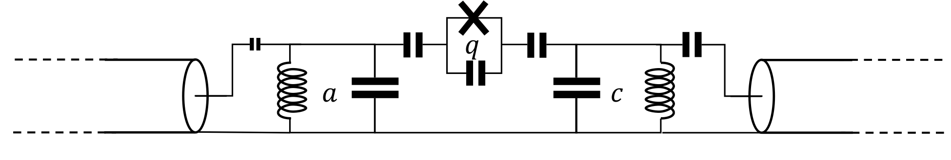
Consider two cavity modes coupled by a single Josephson junction, treated as a qubit mode (see Fig. 9). The resonant frequencies (decay rates) of the three modes are denoted by , . By applying a stiff pump and a weak resonant drive on the mode , for , this system was used for stabilization of Schrödinger cat states. Leghtas et al. (2015) We now show that the same system, for , acts as a degenerate parametric amplifier described in Secs. II, III. We will follow derivation given in the Supplementary Material of Ref. Leghtas et al., 2015.
The total Hamiltonian of the system is given by
| (89) | ||||
Here, are the drive strengths. The frequencies of the incident drives will be determined from the following calculation. Under rotating wave approximation and eliminating the fast dynamics (for details, see Supplementary Material of Ref. Leghtas et al., 2015), we arrive at the resultant Hamiltonian for the modes :
| (90) |
Here, the self-Kerr, cross-Kerr and nonlinear couplings of the modes are respectively given by
| (91) |
where . We have omitted the Hamiltonian terms involving the qubit mode since it does not participate in the dynamics and merely provides the nonlinearity for the interaction between and . Here,
| (92) | ||||
| (93) |
Here, the terms , denote the AC-stark shift due to the presence of the incident pump. To arrive at the degenerate parametric amplifier Hamiltonian [Eq. (39)], we solve for by setting . The resultant Hamiltonian for corresponds to that of the degenerate paramp when the modes are considered in their respective rotating frames. The physical process that underlies the amplification mechanism can be understood easily for negligible cross-Kerr and self-Kerr couplings, when the frequency constraint becomes
| (94) |
Thus, the amplification of the -mode occurs when one photon of the pump (at ) and one photon of the drive (at ) are converted to two photons of the signal (at ).
V.4 Three-mode circuit employing the purely dispersive Josephson 3-wave mixer
We have just described several ways in which a circuit involving Josephson junctions can implement the degenerate parametric amplifier. The non-degenerate parametric amplifier can be implemented by a 3-mode, 3-port circuit employing four junctions forming the so-called Josephson ring modulator, a purely dispersive 3-wave mixer (see Fig. 10 and further details in Ref. Bergeal et al., 2010a, b; Abdo et al., 2013).
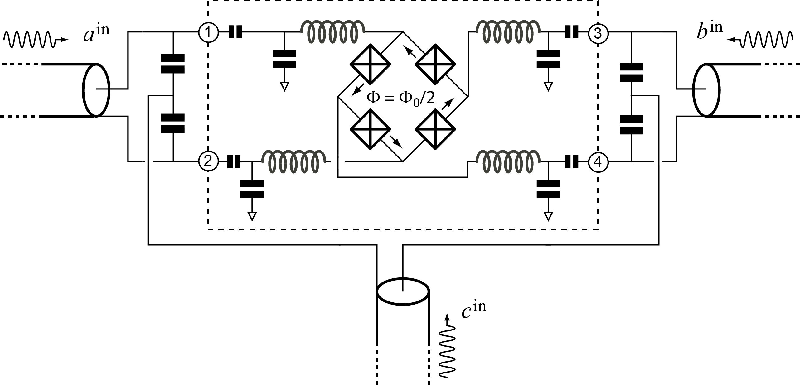
Three microwave standing wave resonators are coupled by this last element and are described by the Hamiltonian
| (95) |
together with their port coupling , and . The frequency scales are such that
| (96) |
The trilinear coupling term, treated as a perturbation, possesses the precious property that it does not, at the lowest order, offset the frequency of the quadratic terms when the modes are occupied by coherent signals, unlike the Kerr term above . Other terms of higher order have been neglected in the Hamiltonian (95). They ensure that the system remains stable when the amplitudes become large, as the trilinear coupling renders by itself the Hamiltonian unstable. In the regime where the mode is driven by a large coherent field , we can neglect the fluctuating part of the corresponding operator. The previous Hamiltonian can be treated as
| (97) |
where
| (98) | |||||
| (99) |
When one works within the framework of the Rotating Wave Approximation and , the fast rotating terms can be neglected and one recovers the Hamiltonian of the generic non-degenerate parametric amplifier
| (100) |
We note that the presence of higher order Kerr nonlinear terms in the Hamiltonian Bergeal et al. (2010a, b) not described here lowers the gain of the device due to AC-stark shift (see discussion at the beginning of Sec. III). A remedy for this drawback has been proposed recently in Refs. Zorin, 2016; Frattini et al., 2017.
VI Related other topics and future directions
Before concluding, we point out several recent amplifier developments which are subject of current research, but were not discussed in this work.
First, a DC and AC flux-driven SQUID performing as an amplifier can be viewed as a nonlinear circuit element, referred to as the “pumpistor”, with a phase-sensitive impedance which can turn negative.Sundqvist et al. (2013) This approach was not presented in this paper since we focussed on the interaction between the signal and the pump, an effect that cannot be addressed by the “pumpistor” idea.
Second, Ref. Roy et al., 2015 proposes an impedance-engineering approach to evade the gain-bandwidth product limitation of amplifiers. In this approach, the nonlinear circuit element based on a Josephson junction is connected to a multi-pole environment. The resulting impedance seen by this element is modified by tuning this environment, thereby providing an additional control to enhance the bandwidth of the amplifier. This impedance-engineering approach is qualitatively different from the one presented in this paper. In contrast to starting with a given Hamiltonian and analyzing its scattering properties, Ref. Roy et al., 2015 starts with a susceptibility function and subsequently, constructs the Hamiltonian and the circuit subjecting the susceptibility function to certain requirements. Thus, while our paper provides the ‘direct’ scattering analysis of a given Hamiltonian, Ref. Roy et al., 2015 provides the ‘inverse’ scattering approach of Hamiltonian construction. Furthermore, the amplifier constructed in this way differs from those presented in this paper in another aspect. Due to the specific form demanded of the susceptibility function of Ref. Roy et al., 2015, the pumped nonlinear part of the circuit sees a fundamentally non-Markovian bath, unlike in the amplifiers described here. Of course, the input-output framework used in our work is powerful enough to model such a non-Markovian environment by considering additional degrees of freedom in the system intercalated between the non-linear element and the transmission line (see Part IV of Ref. Breuer and Petruccione, 2002).
Third, as pointed out in the introduction, a key desired property of an amplifier is its unidirectionality [point (v) of the desiderata]. For the amplifiers described in the body of the paper, additional circuit elements such as circulators and isolators play this crucial function. However, they suffer from the drawback of being lossy and bulky components. Amplifiers which are intrinsically directional and do not suffer from the aforementioned drawbacks have been proposed and for some, realized Kamal et al. (2011); Abdo et al. (2014); Macklin et al. (2015); Ranzani and Aumentado (2015). This is an actively researched topic and goes beyond the scope of this article.
VII Summary
To summarize, we have described in this article degenerate and non-degenerate parametric amplifiers based on Josephson junction circuits. The key organizing concept is the effective quadratic time-dependent Hamiltonian which comes in two forms: degenerate and non-degenerate, depending on whether the signal and idler waves occupy the same physical degree of freedom or two separate ones. In Fig. 11, we summarize the different circuit configurations leading, on one hand, to the degenerate case and, on the other hand, to the non-degenerate case (left and right columns, respectively). The figure also classifies circuits depending on the number of access ports, the simpler case being that of 1-port carrying the signal, idler and pump waves (upper left panels), while the case in which the signal, idler and the pump waves are separated in both temporally and spatially is shown in the bottom right panel. The circuit complexity increases when going from the upper left corner of Fig. 11 to the lower right one. Moreover, we have described the linear scattering properties of these amplifiers in the stiff-pump approximation. Subsequently, we computed the effects of pump depletion and the phase-space properties of signal modes for both degenerate and non-degenerate cases. Finally, we reviewed some practical implementations of such amplifiers.
Acknowledgments
The authors are grateful to Benjamin Huard, Michael Hatridge, Archana Kamal and Katrina Sliwa for valuable discussions in the preparation of this review. AR acknowledges the support through the ERC Consolidator Grant No. 682726 and the support of the Alexander von Humboldt Foundation. AR and MD acknowledge the support of by ARO under Grant No.W911NF-14-1-0011.
Appendix A Quantum signals propagating along a transmission line
Crudely speaking, quantum signals are electromagnetic excitations of a transmission line that involve only a few photons. The state of these excitations must display some degree of quantum purity for the signals to carry quantum information, which is the subject of interest in Josephson circuits. In this section, we provide the basic mathematical background for the concept of quantized electromagnetic excitations in the microwave domain. Gardiner and Zoller (2004); Walls and Milburn (2008) Starting from the microscopic Hamiltonian of a transmission line, we arrive at the concept of left and right moving propagating photon flux operators (see Fig. 12). As will be shown below, they obey the same commutation relations as those of elementary bosonic modes in vacuum. These operators are subsequently used to define the concept of a photonic excitation in a propagating wavepacket.
A.1 Hamiltonian description of a quantum transmission line
Here we follow a route found in previous works (see Chap. 3 of Ref. Drummond and Ficek, 2013, Ref. Gardiner and Zoller, 2004, and Ref. Clerk et al., 2010) with some clarifications particularly necessary for electrical circuits that we hope the reader will find useful. Consider an infinite transmission line, a one-dimensional electromagnetic medium characterized by a propagation velocity and a characteristic impedance . A microwave coaxial line serves as the canonical example of such a medium (see Fig. 13).
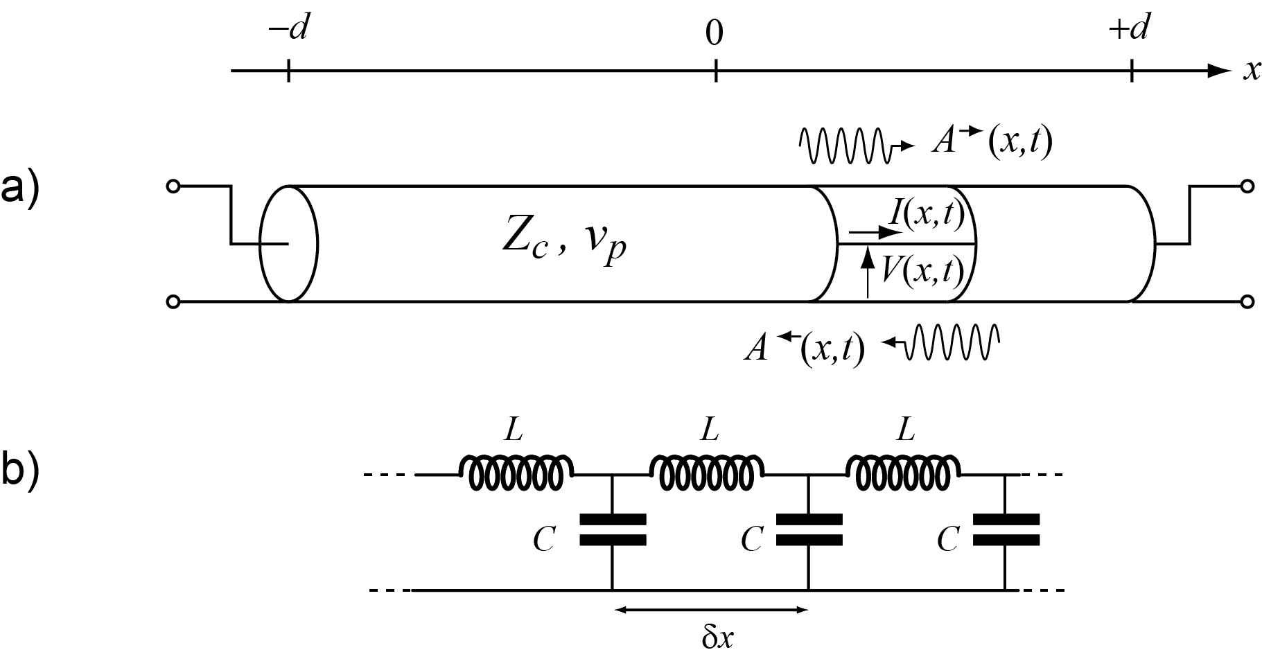
Position along the line is indexed by the real number . We suppose that the line is ideal, with both and independent of frequency . The TEM modes propagating on this transmission line can be equivalently described by propagating modes sustained by the infinite LC ladder shown in Fig. 13 (b), in the limit when the wavelength of the propagating modes are much larger than the size of the unit cell. The inductance and capacitance per unit length are given by: and respectively 444This model of a coaxial transmission line is due to Nyquist and corresponds to an actual microscopic description of the line, where correspond to the inductance and capacitance per unit length of the line. This should be differentiated from the Caldeira-Leggett model of resistance and impedance in terms of an infinite number of LC oscillators. The Caldeira-Leggett model describes the effective behavior of the resistor in terms of the LC oscillators even though underlying microscopic description of the resistor has nothing to do with LC oscillators.. In terms of , the propagating velocity and the characteristic impedance are given by:
| (101) |
Following Ref. [Devoret, 1997], we define a flux operator:
| (102) |
where is the local voltage operator at position on the transmission line at time . The average voltage drop across a segment of length with inductance is . The average flux through the inductance is given by and the operator for the current flowing through the inductance is given by the usual relation:
| (103) |
The Lagrangian that describes the system is given by:
| (104) |
which, through the Euler-Lagrange’s equation of motion, results in the dispersionless wave propagation equation:
| (105) |
The canonical conjugate momentum is the charge density :
| (106) |
and thus, the Hamiltonian describing the transmission is given as:
| (107) |
We define the following Fourier transforms:
| (108) | |||||
| (109) |
Here, the variable denotes the wave-vector of the spatial Fourier component and is not a frequency (the reason for this notation choice will become clear later). The positive and negative values of indicate wave-momentum in and direction, respectively (the red and blue lines of Fig. 12). For a mode propagating with wave-vector , the energy is given by (see below). Also, note that , and not , is the Fourier transform of the charge density. We adopt this notation because the flux and charge operators, and , respectively correspond to the position and momentum operators of the equivalent mechanical system. This choice is appropriate because there are nonlinear, non-dissipative inductances, but no nonlinear, non-dissipative capacitances. Since are Hermitian operators, it follows trivially that:
| (110) |
In terms of the Fourier transformed operators, the Hamiltonian is given by:
| (111) | |||||
where we have used Eq. (101). Next, we define , which plays the role of annihilation operator for different modes of the transmission line:
| (112) |
These operators will be used in turn to define the propagating field operators. Note that with this definition, . Thus, the Hamiltonian can be rewritten in terms of these operators as
| (113) |
Next, we use the canonical quantization relation for the continuous field operators:
| (114) |
which in the Fourier domain, becomes
| (115) |
This leads to the following standard commutation relation for the annihilation field operator :
| (116) |
The Heisenberg equation of motion for the operator is given by:
| (117) | |||||
which can be solved to give:
| (118) |
where is some initial time (eventually, we will take to be ). This, together with Eq. (108), leads to:
| (119) | |||||
| (120) | |||||
Now, we can solve for the field operators arriving at:
| (121) |
| (122) |
Note that, as expected, the operators are Hermitian and have two traveling wave components corresponding to the two opposite traveling directions (see Fig. 12). From these quantities, it is easy to calculate the voltage and current operators using Eqs. (102), (103), leading to:
| (123) | |||||
| (124) |
where
| (125) |
Here, we have expressed the current and voltage operators as superpositions of those operators propagating in opposite directions. As expected, the right(left)-propagating waves involve the operators with positive (negative) wave-vectors. Next, we define the propagating wave amplitude operators in terms of these propagating current and voltage operators:
| (126) | |||||
Eq. (A.1) shows that the spatial dependence can be obtained trivially from by setting :
| (127) | |||||
These simple and physical propagating wave-amplitudes satisfy the following commutation relation:
| (128) |
where according as the denote the direction of propagation is . These traveling wave amplitudes have also been introduced in earlier treatments of input-output theory. Yurke and Denker (1984); Gardiner and Collett (1985); Gardiner and Zoller (2004); Drummond and Ficek (2013) The wave amplitude, whose dimension is [watt]1/2, is such that its square is the energy flux of waves traveling in the direction indicated by the arrow. These propagating wave amplitude operators describe the power-flow in the transmission line. The net power flowing in the direction is given by:
| (129) |
and is equivalent to the usual Poynting vector of electrodynamics. In terms of these propagating wave-amplitudes, the Hamiltonian can be written as:
| (130) |
which expresses the fact that the total energy is the sum of the energies of these propagating waves.
In earlier treatments of dispersionless quantum transmission lines (Chap. 3 of Ref. Drummond and Ficek, 2013, Chap. 3 of Ref. Gardiner and Zoller, 2004, and Ref. Clerk et al., 2010), it is at this point where the rotating wave approximation (RWA) is made before discussing traveling photon wavepackets. These treatments are sufficient when the spectral width of the traveling pulse is much smaller than the center frequency, which is usually the case in usual quantum optical systems operating with center frequencies in the THz range. However, for microwave circuit-QED systems operating with center frequencies in the GHz range, it is easy to conceive of a temporal wave packet that is not well-described by these approximations. Therefore, we go a step further and introduce the concept of a traveling-wave field-ladder operator without making RWA. This is described below.
Define the Fourier transforms of the propagating wave amplitudes as
| (131) |
Here, we have used the squared parenthesis to distinguish the case when the Fourier transform is taken with respect to time from the earlier case when the Fourier transform was with respect to space. Since in a Hermitian operator, it follows that . Using Eqs. (127), (131), one readily obtains:
| (132) | |||||
where the upper (lower) sign in front of correspond to right (left) moving waves. The two signs correspond to the two branches of the blue (leftarrow) and red (rightarrow) lines representing the propagating modes in Fig. 12, while the argument of denotes the position along the branch. These result in the following commutator relation:
| (133) |
which is the frequency-domain counterpart of Eq. (128) and stand for the sense of propagation.
Now, we are ready to define the traveling-wave field ladder operators:
| (134) |
These frequency-domain, traveling-wave, field ladder operators have commutation relations bearing a marked resemblance to the ladder operators of a set of standing wave harmonic oscillators (in the continuum):
| (135) |
This formula represents the central result of this subsection. Note that
| (136) |
In terms of the reciprocal space field operators , these traveling-wave field ladder operators are given by:
| (137) | |||||
| (138) |
As expected, we see that the right(left)-propagating waves involve the field operators with positive (negative) wavevectors. The above equations establish the connection between the traveling field operators defined on the upper and lower half of Fig. 12.
Going back to the time domain, one can evaluate the propagating traveling-wave field ladder operators at to be:
| (139) | |||||
It is important to note that is a Hermitian operator, and it satisfies the commutation relation:
| (140) |
In Appendix B, we will make the rotating wave approximation on this propagating field-operator , which amounts to dropping the second term involving in in Eq. (139).
With the results obtained in this subsection, we can proceed to define propagating photon excitations of the transmission line. This is done below. We emphasize that for defining the photon excitations of the line, we will not need the RWA.
A.2 Definition of a traveling photon wavepacket
In order to properly define the photons of the line, one needs to introduce an orthonormal signal basis consisting of “first-quantization” waveletsMallat (1999) such that
| (141) |
The pair of indices defines a propagating temporal mode of the line, and the combined amplitudes of the two corresponding wavelets can be seen as an elementary degree of freedom of the field. There are two conjugate wavelets per mode since the phase space of each mode is bi-dimensional.
It is necessary to request that the support of , the Fourier transform of , is entirely contained in the positive frequency sector if and in the negative frequency sector if .
| (142) | |||||
| (143) |
In these last expressions, is the Heaviside function 555The index value corresponds to special wavelets that have to be treated separately..
This complete wavelet basis is a purely classical signal processing concept and its existence solely results from the property of the signals to be square-integrable functions. Any continuous signal such that can indeed be decomposed into a countable infinite number of elementary signals
| (144) | |||||
| (145) |
A common example of such a wavelet is the Shannon wavelet
| (146) |
whose Fourier transform is
| (147) |
where is the indicator function which is everywhere except in the interval , where its value is unity. Many other useful bases, involving more continuous wavelets, exist. Mallat (1999) In the above example, the center frequency and time location of the wavelet is and , respectively (in order to form a complete basis, the pitch in frequency and pitch in time of the wavelet basis has to satisfy ) .
The discreteness of the signal component indices is the justification for the term “first-quantization” and no quantum mechanics is involved here since all functions are at this stage c-number valued. Second-quantization intervenes when we define the discrete ladder field operators, with indices and
| (148) | |||||
| (149) | |||||
| (150) |
We introduce the short-hand as the index of the spatio-temporal mode, also called the flying oscillator. The photon-number operator is given by:
| (151) |
and the discrete ladder operators satisfy the same commutation relation as standing mode ladder operators:
| (152) | |||||
An important remark can be made: if the photon amplitude operator is non-hermitian, this is only because its first quantization component is complex. Its second quantization component is an hermitian operator. It is also important to note that, in general, the frequency of a photon is ill-defined, in contrast with what could be inferred from elementary introductions to quantum mechanics. This feature happens as soon as the duration of the wavelet corresponding to that particular photon is not very long compared with the inverse of the wavelet center frequency. Thus the concept of photon for a propagating signal has to be clearly distinguished from an energy quantum. A propagating photon is an elementary excitation of the field carrying a quantum of action, and corresponds to a field wavefunction orthogonal to the vacuum.
| (153) | |||||
| (154) |
A wavelet can contain several photons in mode
| (155) |
and each multi-photon state (Fock state) is orthogonal to the others
| (156) |
Several modes can simultaneously be excited
| (157) |
where the sequence of indices is a mode photon occupancy configuration. Finally, the most general wavefunction of the field of the transmission line is a superposition of all field photon configurations in all the spatio-temporal modes of the line:
| (158) |
There are exponentially many more quantum coefficients than the classical coefficients in Eq. (145)! And it is also important to understand that a state with a well defined number of photons in a certain wavelet basis can be fully entangled in another basis.
A wavelet can also support a so-called coherent state instead of a well defined number of photons:
| (159) | |||||
| (160) |
and if all wavelets are in a coherent state, we obtain a coherent field state
| (161) | |||||
| (162) |
Thus, the set of complex coefficients plays the role of the coefficients in Eq. (145). Somewhat surprisingly, this property of being a coherent state remains true in every wavelet basis (as can be inferred from the quadratic form in the exponent of Eq. [162]).
The state of the line is in general not pure and must be described by a density matrix . This ultimate quantum field description tool leads to the important notion of information contained in the signal.
In general, in quantum mechanics, we can define for a system with a finite-dimension Hilbert space, the ShannonVon Neumann entropy
| (163) |
The information contained in the system is then straightforwardly computed as
| (164) |
where is the fully mixed state in which all basis states are equiprobable, with no off-diagonal correlations. The extension of these ideas to a transmission line on which a signal propagates is not trivial since the number of temporal modes is infinite and each temporal mode has a Hilbert space with infinite dimensionality. Some constraints need to be provided, for instance a fixed total energy for both and . We can also, in another instance, fix the maximum number of excitation in each temporal mode. Supposing that the maximum number of excitations is unity in the domain and that other modes are in the vacuum state, then, for a state of the line characterized by an average photon number per mode
| (165) |
where the information contained in a stochastic binary variable :
| (166) |
We refer the reader to Ref. Holevo, 2013 for a more complete description of the information carried by quantum signals.
A.3 Definition of traveling photon flux
The dimension of the operators is the inverse square root of time and it is tempting to interpret them as photon flux amplitudes. The propagating photon flux in terms of is defined as:
| (167) | |||||
where . Here, is the the photon flux of the incoming drive signal at angular frequency (in units of photons per unit time) and is the Bose occupation factor at the temperature of the electromagnetic excitations of the line. We have supposed that there is only one relevant signal frequency, and the generalization to the case with multiple frequencies is straightforward. Thus, in time-domain, the traveling photon-flux is given by
where we have used Eq. (167). Thus, the first term is the contribution from the thermal and vacuum fluctuations, while the second term is the classical photon flux.
Appendix B Quantum Langevin Equation and Input-Output theory
The main role of the previous section was to introduce the concept of quantum electromagnetic fields propagating along a transmission line at microwave frequencies. The elementary excitations of these fields, microwave photons, can be seen as the carriers of the information transmitted by the propagating field. In this section, we describe how these excitations of the transmission line interact with a localized signal processing device.
We consider a localized signal processing device as a lumped element circuit (, the spatial extent of the scatterer is much smaller than the wavelength of the radiation being scattered) which is connected to two semi-infinite transmission lines [see Fig. 14 (a)]. It receives from the input line the propagating signal carrying the information to be processed and re-emits into the output line another signal carrying the result of the information processing. A crucial ingredient in the description of the mapping of the input signal into the output signal, is the coupling between the circuit, which houses standing electromagnetic modes, and the transmission lines, which support propagating modes. This coupling is dealt with theoretically using the QLE using input-output theory. For simplicity, we consider the situation in which a lumped element circuit with only one electromagnetic mode is coupled to only one semi-infinite transmission line [Fig. 14 (b)]. We will closely follow the form of input-output theory developed in Refs. Gardiner and Collett, 1985; Gardiner and Zoller, 2004 (see also Chap. 3 of Ref. Drummond and Ficek, 2013). In this so-called one-mode, one-port configuration, the signal processing occurs as a transformation of the incoming wave into the reflected outgoing wave. However, in order to utilize the action of the one-mode, one-port circuit, a non-reciprocal linear device called a circulator has to be added in order to separate the incoming and outgoing waves into two independent transmission lines [Fig. 14 (b)]. This circuit configuration also provides a way to model directional, through amplifiers. Courty et al. (1999) We can leave the modeling of the circulator aside for the moment (it is a 3-port device), and derive the equation of motion for an operator of the lumped circuit element.

The input-output formalism also provides a quantum-mechanical model for dissipation in these systems. In microwave circuits, the dissipation can be a resistance connected in series or in parallel (see Fig. 15). In the following section, we derive the QLE for the case when the dissipation is caused by a resistor coupled in series with the circuit. In this case, a voltage source added in series with the resistor is responsible for coherent incident signals and fluctuations. The case when the dissipation is due to a resistor in parallel is treated afterwards. In the latter case, a current source in parallel with the resistor drives coherent incident signals and fluctuations.
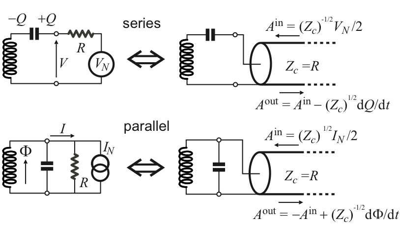
B.1 Dissipation due to a resistor in series, together with a voltage source
B.1.1 Derivation of the Quantum Langevin Equation beyond RWA
Unlike the previous section, we now have a semi-infinite transmission line with characteristic impedance , extending to , coupled to a scatterer (located at ), which we assume to be a lumped circuit with Lagrangian . The total Lagrangian of the system plus transmission line is given by
| (168) |
where are defined as before and is a charge-like system operator that couples to the transmission line with the coupling constant . We have chosen the coupling Hamiltonian so as to ensure that the line voltage couples to X, as necessitated by the insertion of the transmission line in the circuit. The canonical conjugate momentum now has a contribution from the system operator :
| (169) |
The operators still obey the commutation relation:
| (170) |
One can then write down the Hamiltonian for the system and transmission line:
| (171) |
Next, we go to the Fourier domain, by defining the following:
| (172) | |||||
| (173) | |||||
| (174) |
Here, we have involved only the Fourier cosine expansion. This is because for a lumped circuit element, the coupling is local and . Only the Fourier cosine components of and therefore, of couple to the system variable. The operators satisfy the commutation relation
| (175) |
In the Fourier domain, the Hamiltonian of the system and the cosine part of the degrees of freedom of the line reads
| (176) |
The equations of motion for are
| (177) | ||||
| (178) |
We define annihilation operators for the different spatial modes of the transmission line as
| (179) |
which satisfy the commutation relation:
| (180) |
Finally, the Heisenberg equation of motion of is
| (181) |
This can be solved to yield
| (182) | ||||
| (183) |
where is a time far in the past and is a time far in the future. Eventually, we will take and to and respectively so that the dynamics of the circuit takes place entirely in the interval . Now, we can rewrite in terms of the solutions in the past and the future:
which leads to (after some algebra)
| (184) | ||||
| (185) |
where denote input and output fields in the past and the future, defined as
| (186) |
Next, we take to respectively. For a lumped scatterer, the scattered field is outside the region where is nonzero and thus, . Therefore,
| (187) | ||||
| (188) |
Eq. (187) shows that the field at any point is a sum of the input and output fields propagating in opposite directions. Eq. (B.1.1) describes the output fields in terms of the input fields plus some system operator, convolved with the coupling constant. The equation of motion for a system operator is given by
| (189) |
Choosing
| (190) |
leads to
| (191) |
where an extra factor of arises from the integral being from to . From Eq. (B.1.1), setting , we get
| (192) |
Inserting this in Eq. (191), we arrive at
| (193) |
Now, from Eq. (B.1.1), we have
| (194) |
We define incoming and outgoing traveling photon field amplitudes (analogous to those in Sec. A) as and as
| (195) |
Thus, the QLE for the system operator becomes:
| (196) |
In deriving this equation, only the Markov approximation is made, which makes the QLE local in time. This is because we chose the coupling of the form . The RWA has not been made yet (see below). The output field can be computed from the incoming ones using Eq. (187), (192):
| (197) |
We point out that this form of the QLE beyond RWA is useful for analyzing problems such as the spin-boson problemWeiss (1999) or the Kondo problem. Mahan (2013); Le Hur (2012); Goldstein et al. (2013) Next, we perform the RWA on this QLE derived above.
B.1.2 Derivation of the Quantum Langevin Equation under RWA
For simplicity, we will derive the equation for an LC circuit (a harmonic oscillator). It is straightforward to generalize our results to include nonlinearities in our system Hamiltonian. Consider a series LC resonator with inductance and capacitance coupled in series with a resistor with resistance and a voltage source . The suitable choice for the position coordinate of the harmonic oscillator is the charge on the capacitor, denoted by and the corresponding canonically conjugate momentum is the flux through the inductor, denoted by . They obey the commutation relation: . Then, the Hamiltonian for the system is given by
| (198) |
and the coupling operator of the previous section is . Then, the QLE for the operators are:
| (199) | ||||
| (200) |
Now, we define the annihilation operator for the harmonic oscillator as
| (201) |
where is the characteristic impedance of the LC oscillator. Then, the equation of motion of the operator is given by
| (202) |
where is the resonant frequency of the oscillator. Since we are interested in frequencies close to the resonant frequency of the oscillator, we can drop the counter-rotating terms (terms with and ). Further, we can approximate the under the integral with . These two approximations together comprise the RWA. The resultant equation is
| (203) | |||||
Finally, we identify , which is the bandwidth of the resonator. This leaves us with the QLE:
| (204) |
where we have defined
| (205) |
Note that only positive frequencies appear in the definition of the incoming signal. In principle, one can integrate the QLE and express the circuit variable in terms of the incoming field . The output field can be obtained from the input-output equation
| (206) |
Again, the appearance of the simple coefficient in this relation results from the Markov approximation. In the simple case of the harmonic oscillator, the elimination of between input and output can be carried out fully at the analytical level and one obtains
| (207) |
Going to the Fourier domain, one obtains the reflection coefficient
| (208) | |||||
| (209) |
The causality property of the circuit, which expresses the fact that it cannot produce a response before being submitted to a stimulus, is implemented here by the analytic property of the complex function : its pole is in the lower half complex plane while its zero is in the upper half. On the other hand, the property of the reflection coefficient to possess a single pole instead of a pair is an artifact of RWA. As a matter of fact, when the circuit is linear as is the case here, one can compute exactly the reflection coefficient using a more elaborate form of QLE without RWA, while keeping the Markov approximation. One then obtains the expression possessing the necessary pair of poles with values :
| (210) |
It is easy to see that in this last equation, reduces to the single pole expression when is such that and in the underdamped limit .
It is straightforward to generalize our equation for arbitrary system Hamiltonian:
| (211) |
with the boundary condition (for dissipation connected in series)
| (212) |
The remarkably simple form of the QLE is due to the two approximations: i) the Markov approximation which considers that the coupling of the system with the environment is “ohmic”: the density of modes of the environment can be considered white across the set of circuit transition frequencies, as in an ideal resistance, ii) the coupling is also supposed to be weak in the sense that is much smaller than any transition frequency between the energy levels of the lumped circuit. Although approximations are made, the equation respects the important commutation relation of the ladder operators:
| (213) |
at all times .
The incoming driving field has in general three components which are treated on equal footing by the QLE: i) the deterministic signal to be processed, ii) thermal or parasitic noise accompanying the information-carrying signal, and iii) quantum noise, or, in other words, the zero-point fluctuations of the field of the semi-infinite transmission line. The inclusion of this last component is implemented implicitly in that the QLE is an operator equation, in contrast with the Classical Langevin Equation which is just a differential equation for a c-number function, albeit stochastic. Note that the coefficient in front of the propagating field amplitude embodies single-handedly the fluctuation-dissipation theorem: the rate at which energy is radiated away from the circuit (the coefficient of the second term) has to be tightly linked to the coupling constant with which random radiation, emitted from the black body that the line plays the role of, corrupt the purity of the state of the circuit. If one wonders why appears under a square root in this coupling coefficient, one just needs to remember that while is a dimensionless standing photon number amplitude, is the dimensioned amplitude corresponding to a photon flux. Consequently, when the semi-infinite line is in thermal equilibrium (input signal is only black-body noise with temperature ), the following relation involving the anticommutator holds
where is Boltzmann constant, and the average in the thermal state. Given an operating temperature around , this expression shows that the quantum fluctuations become fully dominant over thermal fluctuations at frequencies above a GHz.
B.2 Dissipation due to a resistor in parallel, together with a current source
To compute the QLE for a resistor in parallel (see Fig. 15, lower panel), the derivation presented in Sec. B.1.1, B.1.2 can be used, with some modifications. The suitable variable for the semi-infinite transmission line (impedance and extending to ) is the charge at position , denoted by . The Lagrangian for the total system plus transmission is now given by:
| (214) |
where are defined as before, is the Lagrangian of the system and is now a flux-like system operator that couples to the transmission line with the coupling constant . Then, all the manipulations in Sec. B.1.1 can be done with the substitutions:
| (215) |
For brevity, we skip the steps and present only the results. As before and denote the Fourier cosine-transforms of respectively where is the canonically conjugate momentum of . Note that only in this subsection, correspond to the Fourier transforms of the charge and flux operators of the semi-infinite transmission line. The annihilation operator is defined as
| (216) |
Solving the Heisenberg equation of motion for the annihilation operator and plugging it into the expression for , we get
| (217) | ||||
| (218) |
where denote input and output fields in the past and the future, defined as
| (219) |
The equation of motion for a system operator is given by
| (220) |
Choosing
| (221) |
and noting that
| (222) |
the QLE for the system operator becomes:
| (223) |
This is the QLE for a system coupled to a resistor in parallel, together with a current source where only the Markov approximation has been made. The output field for this case is given by
| (224) |
Note that Eqs. (223, 224) are the parallel connection counterparts of Eqs. (196, 197) given for series connection. Finally, one can perform identical manipulations as in Sec. B.1.2 to arrive at the same QLE under RWA given in Eq. (211):
| (225) |
with the modified boundary condition corresponding to parallel dissipation:
| (226) |
Here, Eqs. (225, 226) are the parallel counterparts of Eqs. (211, 212) given for series coupling.
It is important to note that while the overall form of the QLE under RWA is the same for both kinds of dissipation, both the damping rates and the input-output boundary relations are different. In the case of parallel LC resonator (inductance and capacitance ) coupled to a resistor in parallel, the dissipation rate is . This should be compared with the dissipation rate derived in the series configuration where was equal to . As expected, the dissipation for a series (parallel) configuration increases (decreases) with increasing resistance.
B.3 Generalized QLE for multi-port devices
Continuing to work in the framework of both RWA and the Markov approximation, one can easily deal with more than one circuit mode and more than one semi-infinite line. Denoting by the circuit standing mode index and the port index, one obtains the multi-mode, multi-port generalized QLE:
| (227) |
Apart from a simple extension of the number of variables, this new equation contains the rectangular matrix whose coefficients are . This matrix can be computed from the details of the coupling of the lines to particular elements of the circuit (capacitances or inductances, series or parallel connections). A simple example of a situation where the cannot be set to unity by a re-definition of the mode amplitude is presented in Fig. 16. The general Input-Output Equation takes the form
| (228) |
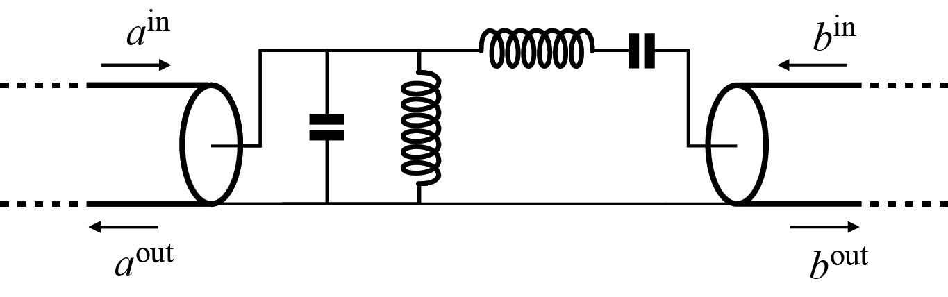
Appendix C Calculation of total output power in parametric amplifiers
C.1 Degenerate case
In this appendix, we outline the calculation of the output power of a degenerate parametric amplifier. We will treat the gain as a parameter, and thus, our results apply to both stiff and depleted calculations. The scattering matrix for this system is given in Eq. (24) of Sec. II. The output power is defined as
| (229) | ||||
In the next step, we substitute the output fields in terms of the input fields using Eq. (24). Thus, we arrive at
Here, , and . For a coherent tone incident on resonance on the -mode, from Eq. (167),
| (230) |
where we have neglected the thermal photon population. Using Eq. (C.1) and keeping only non-vanishing terms,
| (231) |
where we have used that . Simplifying the above equation, we get
| (232) |
which leads to
| (233) |
where
| (234) |
In performing the integral, we have again used . In Eq. (233), the first term is the amplified classical power. The second term in the output power arises from vacuum fluctuations, amplified by a factor , integrated over the effective bandwidth .
C.2 Non-degenerate case
The output power for the non-degenerate case proceeds analogously and in the case when only the signal mode is driven, one arrives at
| (235) |
where
| (236) |
Appendix D Dynamic range results for the degenerate parametric amplifier
In this section, we present the results of the calculations of the gain, output power and shift of threshold for the parametric oscillation in the degenerate parametric amplifier. The behaviors of these quantities are completely analogous to the non-degenerate case presented in the main text.
Fig. 17 shows the resultant gain of the device as a function of coherent incident signal power (). The different curves correspond to un-depleted gain of to dB, in steps of dB.
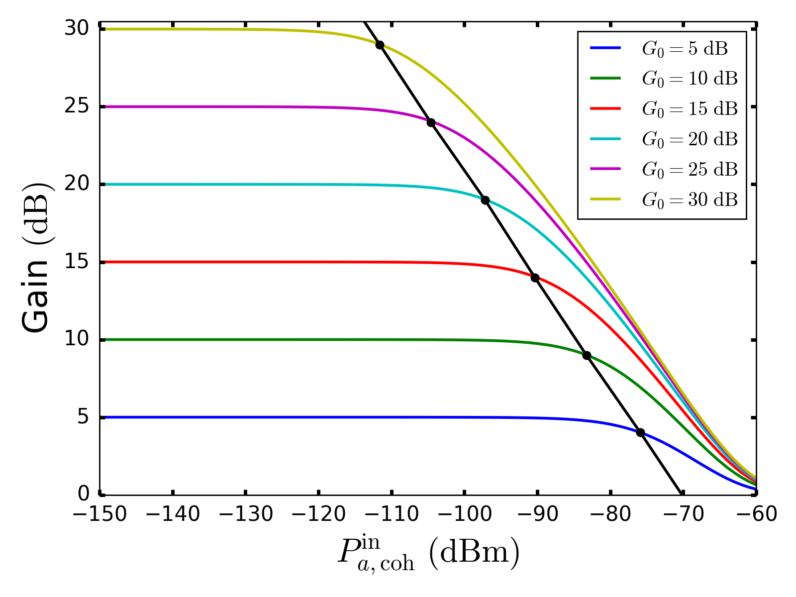
In Fig. 18, the total output signal power is plotted as a function of . The solid curves denote the output power for un-depleted gain of to dB, in steps of dB. As the incident coherent signal power goes to zero, the output power saturates and corresponds to amplified vacuum fluctuations incident on the signal port. The black dot-dashed line correspond to zero un-depleted gain when the pump tone is switched off. Finally, the dashed black line correspond the maximum output power that the device can produce before the onset of spontaneous parametric oscillation.
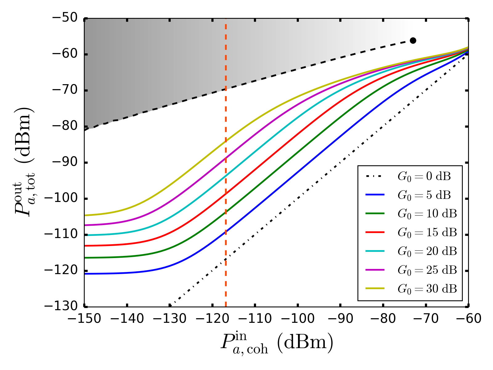
As incident signal power is increased, the pump power needed for onset of oscillation, the threshold pump power, increases. This is shown in Fig. 19. For sufficiently high incident signal power, the system ceases to exhibit parametric oscillation (denoted by the black circle in Figs. 18, 19).
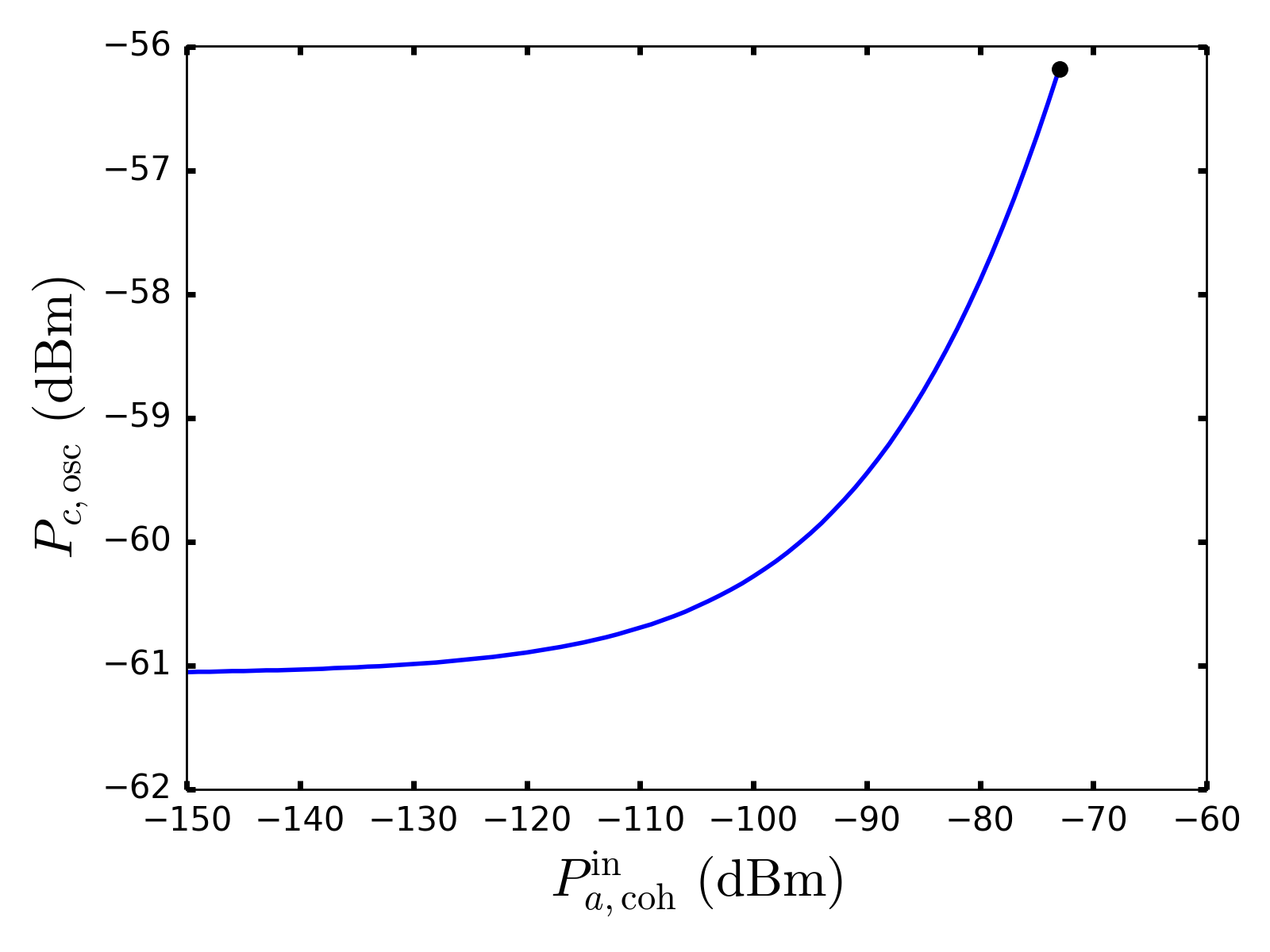
References
- Devoret and Schoelkopf (2013) M. H. Devoret and R. J. Schoelkopf, Science 339, 1169 (2013).
- Caves (1982) C. M. Caves, Phys. Rev. D 26, 1817 (1982).
- Yurke et al. (1988) B. Yurke, P. G. Kaminsky, R. E. Miller, E. A. Whittaker, A. D. Smith, A. H. Silver, and R. W. Simon, Phys. Rev. Lett. 60, 764 (1988).
- Yurke et al. (1989) B. Yurke, L. R. Corruccini, P. G. Kaminsky, L. W. Rupp, A. D. Smith, A. H. Silver, R. W. Simon, and E. A. Whittaker, Phys. Rev. A 39, 2519 (1989).
- Vijay et al. (2011) R. Vijay, D. H. Slichter, and I. Siddiqi, Phys. Rev. Lett. 106, 110502 (2011).
- Hatridge et al. (2013) M. Hatridge, S. Shankar, M. Mirrahimi, F. Schackert, K. Geerlings, T. Brecht, K. M. Sliwa, B. Abdo, L. Frunzio, S. M. Girvin, R. J. Schoelkopf, and M. H. Devoret, Science 339, 178 (2013).
- Kamal et al. (2009) A. Kamal, A. Marblestone, and M. Devoret, Phys. Rev. B 79, 184301 (2009).
- Bergeal et al. (2010a) N. Bergeal, R. Vijay, V. E. Manucharyan, I. Siddiqi, R. J. Schoelkopf, S. M. Girvin, and M. H. Devoret, Nat Phys 6, 296 (2010a).
- Abdo et al. (2013) B. Abdo, A. Kamal, and M. Devoret, Phys. Rev. B 87, 14508 (2013).
- Roy and Devoret (2016) A. Roy and M. Devoret, Comptes Rendus Physique 17, 740 (2016), quantum microwaves / Micro-ondes quantiques.
- Walls and Milburn (2008) D. F. Walls and G. J. Milburn, Quantum Optics, SpringerLink: Springer e-Books (Springer, 2008).
- Drummond and Ficek (2013) P. D. Drummond and Z. Ficek, Quantum Squeezing, Springer Series on Atomic, Optical, and Plasma Physics (Springer Berlin Heidelberg, 2013).
- Liu et al. (2017) G. Liu, T.-C. Chien, X. Cao, O. Lanes, E. Alpern, D. Pekker, and M. Hatridge, Applied Physics Letters 111, 202603 (2017), https://doi.org/10.1063/1.5003032 .
- Zorin (2016) A. B. Zorin, Phys. Rev. Applied 6, 034006 (2016).
- Frattini et al. (2017) N. E. Frattini, U. Vool, S. Shankar, A. Narla, K. M. Sliwa, and M. H. Devoret, Applied Physics Letters 110, 222603 (2017), https://doi.org/10.1063/1.4984142 .
- Note (1) For similar analysis in a related topic, see Refs. \rev@citealpnumLahteenmaki2013, Lahteenmaki2016.
- Note (2) Such a trilinear Hamiltonian arises also in treatment of Hawking radiation from a quantized source Nation and Blencowe (2010).
- Note (3) This curve can be obtained as follows. Solving the coupled nonlinear set of equations [Eqs. (34, 35, 36)] in steady state, one obtains the smallest pump power which gives rise to multiple, stable, steady-state solutions for the modes . The pump power immediately below this value is the maximum allowed pump power. In practice, the equations are solved numerically for different pump powers.
- Carmichael (2007) H. Carmichael, Statistical Methods in Quantum Optics 2: Non-Classical Fields, Statistical Methods in Quantum Optics (Springer, 2007).
- Carmichael (1999) H. Carmichael, Statistical Methods in Quantum Optics 1: Master Equations and Fokker-Planck Equations, Physics and Astronomy Online Library (Springer, 1999).
- Reid and Drummond (1989) M. D. Reid and P. D. Drummond, Phys. Rev. A 40, 4493 (1989).
- Siddiqi et al. (2004) I. Siddiqi, R. Vijay, F. Pierre, C. M. Wilson, M. Metcalfe, C. Rigetti, L. Frunzio, and M. H. Devoret, Phys. Rev. Lett. 93, 207002 (2004).
- Vijayaraghavan (2008) R. Vijayaraghavan, Ph.D. Thesis (Yale University, 2008).
- Manucharyan et al. (2007) V. E. Manucharyan, E. Boaknin, M. Metcalfe, R. Vijay, I. Siddiqi, and M. Devoret, Phys. Rev. B 76, 14524 (2007).
- Nigg et al. (2012) S. E. Nigg, H. Paik, B. Vlastakis, G. Kirchmair, S. Shankar, L. Frunzio, M. H. Devoret, R. J. Schoelkopf, and S. M. Girvin, Phys. Rev. Lett. 108, 240502 (2012).
- Castellanos-Beltran et al. (2008) M. A. Castellanos-Beltran, K. D. Irwin, G. C. Hilton, L. R. Vale, and K. W. Lehnert, Nat Phys 4, 929 (2008).
- Castellanos-Beltran et al. (2009) M. A. Castellanos-Beltran, K. D. Irwin, L. R. Vale, G. C. Hilton, and K. W. Lehnert, IEEE Transactions on Applied Superconductivity, IEEE Transactions on Applied Superconductivity 19, 944 (2009).
- Macklin et al. (2015) C. Macklin, K. O’Brien, D. Hover, M. E. Schwartz, V. Bolkhovsky, X. Zhang, W. D. Oliver, and I. Siddiqi, Science 350, 307 (2015).
- Yamamoto et al. (2008) T. Yamamoto, K. Inomata, M. Watanabe, K. Matsuba, T. Miyazaki, W. D. Oliver, Y. Nakamura, and J. S. Tsai, Applied Physics Letters 93, (2008).
- Johansson et al. (2009) J. R. Johansson, G. Johansson, C. M. Wilson, and F. Nori, Phys. Rev. Lett. 103, 147003 (2009).
- Zhong et al. (2013) L. Zhong, E. P. Menzel, R. D. Candia, P. Eder, M. Ihmig, A. Baust, M. Haeberlein, E. Hoffmann, K. Inomata, T. Yamamoto, Y. Nakamura, E. Solano, F. Deppe, A. Marx, and R. Gross, New Journal of Physics 15, 125013 (2013).
- Zhou et al. (2014) X. Zhou, V. Schmitt, P. Bertet, D. Vion, W. Wustmann, V. Shumeiko, and D. Esteve, Phys. Rev. B 89, 214517 (2014).
- Mutus et al. (2014) J. Y. Mutus, T. C. White, R. Barends, Y. Chen, Z. Chen, B. Chiaro, A. Dunsworth, E. Jeffrey, J. Kelly, A. Megrant, C. Neill, P. J. J. O Malley, P. Roushan, D. Sank, A. Vainsencher, J. Wenner, K. M. Sundqvist, A. N. Cleland, and J. M. Martinis, Applied Physics Letters 104 (2014), http://dx.doi.org/10.1063/1.4886408.
- Leghtas et al. (2015) Z. Leghtas, S. Touzard, I. M. Pop, A. Kou, B. Vlastakis, A. Petrenko, K. M. Sliwa, A. Narla, S. Shankar, M. J. Hatridge, M. Reagor, L. Frunzio, R. J. Schoelkopf, M. Mirrahimi, and M. H. Devoret, Science 347, 853 (2015).
- Bergeal et al. (2010b) N. Bergeal, F. Schackert, M. Metcalfe, R. Vijay, V. E. Manucharyan, L. Frunzio, D. E. Prober, R. J. Schoelkopf, S. M. Girvin, and M. H. Devoret, Nature 465, 64 (2010b).
- Sundqvist et al. (2013) K. M. Sundqvist, S. Kintaş, M. Simoen, P. Krantz, M. Sandberg, C. M. Wilson, and P. Delsing, Applied Physics Letters 103, 102603 (2013), https://doi.org/10.1063/1.4819881 .
- Roy et al. (2015) T. Roy, S. Kundu, M. Chand, A. M. Vadiraj, A. Ranadive, N. Nehra, M. P. Patankar, J. Aumentado, A. A. Clerk, and R. Vijay, Applied Physics Letters 107, 262601 (2015).
- Breuer and Petruccione (2002) H. Breuer and F. Petruccione, The Theory of Open Quantum Systems (Oxford University Press, 2002).
- Kamal et al. (2011) A. Kamal, J. Clarke, and M. H. Devoret, Nat Phys 7, 311 (2011).
- Abdo et al. (2014) B. Abdo, K. Sliwa, S. Shankar, M. Hatridge, L. Frunzio, R. Schoelkopf, and M. Devoret, Phys. Rev. Lett. 112, 167701 (2014).
- Ranzani and Aumentado (2015) L. Ranzani and J. Aumentado, New J. Phys. 17, 23024 (2015).
- Metelmann and Clerk (2014) A. Metelmann and A. A. Clerk, Phys. Rev. Lett. 112, 133904 (2014).
- Gardiner and Zoller (2004) C. Gardiner and P. Zoller, Quantum Noise: A Handbook of Markovian and Non-Markovian Quantum Stochastic Methods with Applications to Quantum Optics, Springer Series in Synergetics (Springer, 2004).
- Clerk et al. (2010) A. A. Clerk, M. H. Devoret, S. M. Girvin, F. Marquardt, and R. J. Schoelkopf, Rev. Mod. Phys. 82, 1155 (2010).
- Note (4) This model of a coaxial transmission line is due to Nyquist and corresponds to an actual microscopic description of the line, where correspond to the inductance and capacitance per unit length of the line. This should be differentiated from the Caldeira-Leggett model of resistance and impedance in terms of an infinite number of LC oscillators. The Caldeira-Leggett model describes the effective behavior of the resistor in terms of the LC oscillators even though underlying microscopic description of the resistor has nothing to do with LC oscillators.
- Devoret (1997) M. H. Devoret, Quantum Fluctuations in Electrical Circuits (Les Houches Session LXIII) (Elsevier, 1997) pp. 351–386.
- Yurke and Denker (1984) B. Yurke and J. S. Denker, Phys. Rev. A 29, 1419 (1984).
- Gardiner and Collett (1985) C. W. Gardiner and M. J. Collett, Phys. Rev. A 31, 3761 (1985).
- Mallat (1999) S. Mallat, A Wavelet Tour of Signal Processing, Wavelet Tour of Signal Processing (Elsevier Science, 1999).
- Note (5) The index value corresponds to special wavelets that have to be treated separately.
- Holevo (2013) A. S. Holevo, Quantum Systems, Channels, Information: A Mathematical Introduction, De Gruyter Studies in Mathematical Physics (De Gruyter, 2013).
- Courty et al. (1999) J.-M. Courty, F. Grassia, and S. Reynaud, EPL (Europhysics Letters) 46, 31 (1999).
- Weiss (1999) U. Weiss, Quantum Dissipative Systems, Series in modern condensed matter physics (World Scientific, 1999).
- Mahan (2013) G. Mahan, Many-Particle Physics, Physics of Solids and Liquids (Springer US, 2013).
- Le Hur (2012) K. Le Hur, Phys. Rev. B 85, 140506 (2012).
- Goldstein et al. (2013) M. Goldstein, M. H. Devoret, M. Houzet, and L. I. Glazman, Phys. Rev. Lett. 110, 017002 (2013).
- Lähteenmäki et al. (2013) P. Lähteenmäki, G. S. Paraoanu, J. Hassel, and P. J. Hakonen, Proceedings of the National Academy of Sciences 110, 4234 (2013), http://www.pnas.org/content/110/11/4234.full.pdf .
- Lähteenmäki et al. (2016) P. Lähteenmäki, G. S. Paraoanu, J. Hassel, and P. J. Hakonen, Nature Communications 7, 12548 EP (2016).
- Nation and Blencowe (2010) P. D. Nation and M. P. Blencowe, New Journal of Physics 12, 095013 (2010).