Task-based Parallel Computation of the Density Matrix in Quantum-based Molecular Dynamics using Graph Partitioning

Abstract

Quantum-based molecular dynamics (QMD) is a highly accurate and transferable method for material science simulations. However, the time scales and system sizes accessible to QMD are typically limited to picoseconds and a few hundred atoms. These constraints arise due to expensive self-consistent ground-state electronic structure calculations that can often scale cubically with the number of atoms. Linearly scaling methods depend on computing the density matrix $\mathbf{P}$ from the Hamiltonian matrix $\mathbf{H}$ by exploiting the sparsity in both matrices. The second-order spectral projection (SP2) algorithm is an $O(N)$ algorithm that computes $\mathbf{P}$ with a sequence of $40-50$ matrix-matrix multiplications. In this paper, we present task-based implementations of a recently developed data-parallel graph-based approach to the SP2 algorithm, G-SP2. We represent the density matrix $\mathbf{P}$ as an undirected graph and use graph partitioning techniques to divide the computation into smaller independent tasks. The partitions thus obtained are generally not of equal size and give rise to undesirable load imbalances in standard MPI-based implementations. This load-balancing challenge can be mitigated by dynamically scheduling parallel computations at runtime using task-based programming models. We develop task-based implementations of the data-parallel G-SP2 algorithm using both Intel’s Concurrent Collections (CnC) as well as the Charm++ programming model and evaluate these implementations for future use. Scaling and performance results of our implementations are investigated for representative segments of QMD simulations for solvated protein systems containing more than $10,000$ atoms.

1 Introduction

Quantum-based molecular dynamics (QMD) simulations of large physical systems are limited due to the high cost of electronic structure calculations, which often involves determining the eigenstates of the Hamiltonian matrix $\mathbf{H}$. Traditional electronic structure calculations rely on methods such as direct diagonalization, gradient based energy minimization schemes [13], or Chebyshev filtering techniques [35, 1] that scale as $O(N^{3})$, where $N$ denotes the size of the Hamiltonian $\mathbf{H}$. However, instead of individual eigenstates of $\mathbf{H}$, often the density matrix $\mathbf{P}$, which is the sum of the outer product of eigenstates of $\mathbf{H}$, is desired. Elements of $\mathbf{P}$ decay exponentially away from the diagonal for gapped systems and metals at finite temperature, while elements of $\mathbf{P}$ decay algebraically for metallic systems at zero temperature [15, 20]. The nearsightedness of physical systems, which results in sparse $\mathbf{P}$, makes electronic structure calculations that scale as $O(N)$ possible. An overview of common approaches can be found in the literature, particularly [4, 16].

The second-order spectral projection purification method (SP2) is an $O(N)$ algorithm to compute the density matrix $\mathbf{P}$ for any Hamiltonian $\mathbf{H}$. In comparison to other $O(N)$ methods, the advantage of SP2 is that its $O(N)$ scaling is not tied to the method used to generate $\mathbf{H}$. SP2 does not require construction of Wannier-like functions with an imposed localization constraint as in [33, 18], and it also differs from finite-difference based electronic structure calculations that impose localization constraints on numerical solutions [11] to obtain $O(N)$ scaling. While the aforementioned approaches have been shown to be accurate and scaleable, their $O(N)$ scaling is coupled to the choice of basis sets and imposed localization constraints. On the other hand, given any $\mathbf{H}$, SP2 can be used to obtain $\mathbf{P}$ with $O(N)$ computational cost, as long as the matrices are sparse.

SP2 replaces matrix diagonalization by a sequence of matrix-matrix multiplications with approximate $O(N)$ [25] complexity if a numerically thresholded sparse-matrix algebra is used. Dense SP2 calculations also run efficiently on heterogeneous architectures that include graphics processing units (GPUs) within a single-node environment [8, 9]. However, running the sequential SP2 algorithm on multi-node distributed-memory architectures requires storing, communicating, and updating matrices after every multiplication, and leads to significant overhead even with the help of sparse matrix libraries such as DBCSR [3], and SpAMM [2]. Performance can be improved by noting that if an initial $\mathbf{P}$ is known, the sparse structure of subsequent density matrices remains unchanged over several self-consistency or MD steps. Recently, graph theory was used to re-design the SP2 algorithm so that $\mathbf{H}$ can be divided into smaller matrices such that independent SP2 iterations can be done in a data-parallel way, resulting in substantial performance gains [26].

The graph-based data-parallel version of the SP2 algorithm (hereafter denoted as G-SP2) can significantly improve performance simply by using off-the-shelf graph partitioning methods [26]. However, it was found that the subgraphs obtained from off-the-shelf graph partitioning are often of unequal size [10], which can lead to significant load imbalances in a parallel implementation. These imbalances show wide variability depending on the physical system being studied. For instance, solvated proteins and molecular crystals may have sparse $\mathbf{P}$ but their chemical connectivity varies. If the same QMD application is to simulate different physical systems efficiently, load balancing should be automated. This becomes a particularly challenging problem in the strong scaling limit, which is needed to reach a low wall-clock time per calculated QMD time step. In this paper, we explore how runtime systems can be used for automatic load-balancing in G-SP2 calculations to fully exploit computing resources. We extend the methods presented in [26, 10], which were designed to minimize the total computational cost of density matrix calculations via G-SP2 but without any considerations about the details of the parallel framework.

1.1 Parallel implementation of G-SP2

Figure 1: Schematic for the proposed data-parallel G-SP2 algorithm in a QMD application such as LATTE. The runtime system uses the partitioned graph to divide the SP2 calculation into independent dense matrix-matrix multiplication subproblems. These subproblems are assigned to processors using a task-based scheduler such as CnC [5] or Charm++ [30]. The resulting $\mathbf{P}$ is collected and sent back to the QMD application.

Fig. 1 shows a schematic of our proposed parallel implementation of the G-SP2 algorithm using a task-based runtime system. Initially, an external QMD method, such as the self-consistent density functional tight-binding scheme as implemented in LATTE [32], computes the self-consistent Hamiltonian matrix $\mathbf{H}$ and its corresponding density matrix $\mathbf{P}$. This is done using the standard numerically thresholded sparse SP2 scheme, which is hard to parallelize over many nodes. The non-zero structure of the thresholded density matrix $\mathbf{P}$ is then used to determine the adjacency matrix of a graph that approximates the data dependencies in the Fermi-operator expansion. Partitioning algorithms are used to divide the graph into subgraphs that are used to extract submatrices of $\mathbf{H}$ corresponding to independent small dense subproblems. The subproblems identified through graph partitioning serve as inputs to a runtime system that dynamically schedules dense matrix SP2 computations that run independently until convergence. The resulting submatrices are collected and reassembled to form the full density matrix $\mathbf{P}$, which is subsequently used to estimate the data dependency graph and partitioning for the next time step, possibly adding or removing data dependencies as the atoms have moved.

Simulated material systems do not exhibit rapid changes on the order of the integration step size, meaning that the graph structure extracted from $\mathbf{P}$ is largely preserved over several time steps. It is therefore reasonable to reuse a particular set of graph partitions over a user-specified number of time steps $n$ chosen with respect to the system kinetics and dynamics. This is analogous to periodically updated neighbor lists for computing pairwise interactions in standard MD implementations [12]. The variable $i$ in Fig. 1 serves as an iteration counter: in each iteration $i$, a new $\mathbf{P}$ is computed at time $t_{i}$ in a parallel fashion. However, the partitions are only re-computed every $n$ steps (i.e., the branch $i=0$ (mod) $n$ is executed). Otherwise, $\mathbf{P}$ is computed according to the existing (old) partitions corresponding to the branch $i\neq 0$ (mod) $n$.

2 Methods

2.1 Second-Order Spectral Projection Method (SP2)

The SP2 algorithm [28] computes $\mathbf{P}$ via matrix multiplications without explicitly computing the chemical potential $\mu$ or the eigenstates of $\mathbf{H}$. The SP2 algorithm starts from an initial guess for the density matrix, $\mathbf{X}_{0}$, which is a rescaled Hamiltonian

$$\mathbf{X}_{0}=\frac{\epsilon_{\text{max}}\mathbf{I}-\mathbf{H}}{\epsilon_{\text{max}}-\epsilon_{\text{min}}},$$ (1)

whose eigenvalues are mapped to the interval $[0,1]$ in reverse order. Estimates of the minimum ($\epsilon_{\text{min}}$) and maximum ($\epsilon_{\text{max}}$) eigenvalues of $\mathbf{H}$ were obtained from the Gershgorin circle theorem [14]. Gershgorin circles can be used here because only the maximum and minimum bounds, and not their accurate values are required. At each iteration $i$, an $\mathbf{X}_{i}$ is obtained from the previous estimate $\mathbf{X}_{i-1}$ using

$$\mathbf{X}_{i}=\left[\mathbf{I}+\alpha_{i}(\mathbf{I}-\mathbf{X}_{i-1})\right]\mathbf{X}_{i-1}.$$ (2)

Here, $\alpha_{i}=1$ if $2\text{Tr}[\mathbf{X}_{i}]\leq N_{\text{el}}$, where $N_{\text{el}}$ denotes the number of electrons of the physical system, and $\alpha_{i}=-1$ otherwise. In self-consistent charge tight-binding, the initial density matrix is computed using regular SP2 from which we store the multiplication sequence determined by $\{\alpha_{i}\}_{i=1,2,\ldots}$. This sequence of multiplications can be used to compute the density matrix during the iterative refinement of $\mathbf{H}$ and $\mathbf{P}$. The same sequence is used either until convergence of the self-consistent charge procedure or for a fixed number of iterations. In case the sequence of $\alpha_{i}$ is wrong, the iteration ends with the wrong trace, and the sequence has to be recomputed. $\mathbf{P}$ is obtained in the limit

$$\mathbf{P}=\lim_{i\rightarrow\infty}\mathbf{X}_{i}.$$ (3)

A criterion to check the convergence in eq. (3) is to verify that $\mathbf{P}$ is idempotent (i.e., $\mathbf{P}^{2}=\mathbf{P}$) within given error bounds [27]. In our examples, a few dozen iterations were usually sufficient to compute $\mathbf{P}$, even for systems as large as $\sim 10,000$ atoms.

2.2 Graph Theory

After the initial density matrix $\mathbf{P}$ has been computed using regular SP2, a graph $G_{\tau}=(V,E)$ with vertex set $V$ and edge set $E$ is constructed by using the non-zero structure of $\mathbf{P}$ thresholded with a global parameter $\tau$ [26]. Each row (or column, since $\mathbf{P}$ is symmetric) of $\mathbf{P}$ corresponds to a vertex $v$ in the graph. Pairs of vertices $u$ and $v$ will be connected through an edge $(u,v)$ in $E$ if $|\mathbf{P}_{u\,v}|>\tau$. The threshold $\tau$ is a parameter used in both graph-based and standard [7] SP2 implementations which allows for a well-controlled tuning of the computational error.

Graph partitioning algorithms divide a graph into distinct partitions while attempting to minimize a variety of metrics. Let $G$ be an undirected graph and $n\geq 2$ be an integer denoting the number of partitions (or equivalently, subproblems). We call any vertex belonging to a given graph partition a core vertex of that partition. Additionally, we are interested in the set of all vertices that do not belong to the partition, but are connected neighbors of any of the core vertices. We will call any such vertex a halo vertex of the partition. Each G-SP2 subproblem $i$ is comprised of $c_{i}$ core vertices and $h_{i}$ halo vertices in neighboring partitions, so its size is $s_{i}=c_{i}+h_{i}$. We are interested in partitioning $G$ into $n$ partitions in a way that minimizes the objective function

$$C(\{c_{i}\},\{h_{i}\};n)=\sum_{i=1}^{n}(c_{i}+h_{i})^{3},$$ (4)

which is the total computational cost for the G-SP2 subproblems. (Or more precisely, the total cost of the corresponding dense matrix-matrix multiplications for each submatrix of $\mathbf{P}$ corresponding to a partition.) Partitioning a graph with respect to the objective function in eq. (4) was called CH-partitioning (core-halo partitioning) in [10]. Note that this objective function differs from the one employed in traditional edge-cut minimization [22, 31]. We observe this by investigating two partitionings (each with two partitions) of a simple graph in Fig. 2.

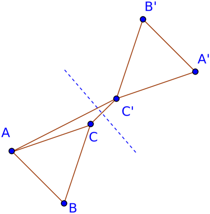
(a) Each partition has three core vertices and one neighbor vertex in the other partition.

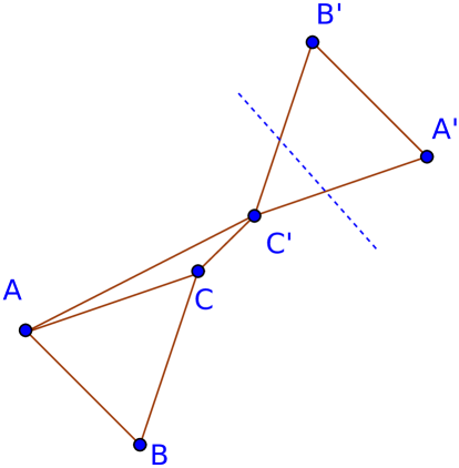
(b) One partition has 4 core vertices and two neighbors. Another partition has two cores and one neighbor.

Figure 2: Two ways to partition the same graph resulting in equal edge-cuts but with different subproblem sizes. The computational cost of G-SP2 is proportional to the cubed sum of the number of vertices and neighbors in each partition. The partitioning shown in (a) is thus preferred.

In the first scenario (Fig. 2), the two partitions consist of the vertices $(A,B,C)$ and $(A^{\prime},B^{\prime},C^{\prime})$, respectively. In the second scenario (Fig. 2), the graph is divided into partitions containing $(A,B,C,C^{\prime})$ and $(A^{\prime},B^{\prime})$. Edge-cut minimization cannot distinguish between the cases depicted in Figs. 2 and 2 because the number of edges between the two partitions is two in both cases.

In Fig. 2, one of the two G-SP2 subproblem has core vertices $A$, $B$, and $C$ and halo vertex $C^{\prime}$ while the other has core vertices $A^{\prime}$, $B^{\prime}$, and $C^{\prime}$ and halo vertices $A$ and $C$. This results in two submatrices of dimension $4$ and $5$ respectively. In Fig. 2, one subproblem contains four core vertices and two halo vertices, whereas the other subproblem contains two core and one halo vertex, resulting in two submatrices of dimension $6$ and $3$, respectively. The computational cost for G-SP2 using Fig. 2 is proportional to $4^{3}+5^{3}=189$, while the computational cost for Fig. 2 is proportional to $6^{3}+3^{3}=243$.

In [10], the standard graph partitioning software packages METIS [22], KaHIP [31] and hMETIS [23] were evaluated with respect to their performance in computing efficient CH-partitionings. In addition, an approach based on simulated annealing (SA) designed to minimize eq. (4) was also evaluated. From [10], we conclude that in practice, METIS was most suitable for efficiently minimizing eq. (4) and thus for computing CH-partitionings on a variety of test graphs. Simulated annealing almost always improved the quality of partitions, and was more useful for dense graphs. However, using SA could lead to more load imbalances, as entire partitions were ’dissolved’ in some cases in order to improve the numerical cost metric. Thus, METIS was used to partition graphs for all the results presented in this manuscript.

Finally, we note that independent subproblems can also be constructed by using locality – core vertices in partitions can be chosen based on locality, and given these core vertices, there will be a localization radius beyond which elements of $\mathbf{P}$ can be set to zero as in [11] – but graph partitioning provides a more general way to obtain partitions (e.g., by partitioning using an objective function which can, but does not need to, depend on distances). Grouping matrix elements according to their interaction strengths in $\mathbf{P}$ rather than the distance can be especially useful for sparse and heterogeneous simulations cells, where distance-based cutoffs may result in larger submatrices than necessary.

2.3 Asynchronous Programming Models

G-SP2 allows us to divide a large sequential problem into smaller data-parallel subproblems that can be scheduled using a Bulk Synchronous Parallel (BSP) implementation: for instance, by using MPI (message passing interface) and OpenMP threading. This approach is sufficient for uniform systems, where subproblems can be expected to be of similar sizes, or when a specific physical system is being targeted so that possible load imbalances are known a priori and can be mitigated. However, for a general application used to study systems with a variety of bonding configurations a greater variability in subproblem sizes is expected, and it is for these systems that asynchronous parallel programming based G-SP2 will be most useful. The type and severity of load imbalance varies with the physical system being studied; this rules out hard-coding a scheduler or load balancer.

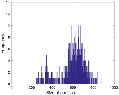
Figure 3: Distribution of G-SP2 subproblem matrix sizes obtained using simple block partitioning applied to the density matrix of polyalanine 289 having dimension $\sim 40,000$.

Fig. 3 shows an example for the distribution of G-SP2 subproblem sizes where load-balancing can be useful. The density matrix of polyalanine 289 with $41185$ vertices, one of the test matrices used in [10], was block partitioned into 1200 partitions. By block partitioning, we refer to a simple technique which allocates a fixed number of cores (or orbitals) to each partition in order of their appearance in the Hamiltonian matrix. For the polyalanine molecule, each partition either has $34$ or $35$ cores. Although each partition contains about the same number of core vertices, the number of halo vertices for each partition differs significantly and affects the subproblem size. In more densely connected graphs, each core vertex has more neighbors so that given an equal number of core vertices per partition, subproblems are likely to be larger, and the distribution in Fig. 3 shifts to the right. Similarly, for heterogenous systems with the same core vertices in each partition, but with coexisting sparsely and densely connected regions, a wider distribution of subproblem sizes is expected.

3 Results

3.1 Selection of a runtime system

Asynchronous parallel programming is relatively new to scientific applications so we investigated two asynchronous task-based runtime systems, namely Intel Concurrent Collections CnC [5] and Charm++ [30], to schedule and execute SP2 subproblems. Detailed descriptions of CnC and Charm++ are found in Appendix A. The Los Alamos National Laboratory CentOS cluster Darwin, which has a highly heterogeneous architecture with four 18-core Intel Xeon E7-8880 v3 CPUs clocked at 2.3 GHz and 512 GB of RAM, was used. Hyper-threading was disabled so that each node had 72 cores and 72 threads. All runtimes in this and the following sections are for a single density matrix computation.

Fig. 4 shows the time taken for a single density matrix computation as a function of the number of partitions for two different systems. Runtimes on the left y-axis correspond to a 3D-periodic simulation cell containing liquid water with density matrix of size $\sim 6000$, while runtimes on the right y-axis correspond to a unit cell of protein solvated in water with $\mathbf{P}$ of size $\sim 31,000$. Arrows within Fig. 4 indicate the largest subproblem sizes, which represent the most expensive linear algebra computations, for the specified numbers of partitions and for both simulation cells. We note that partitioning the SP2 calculation into subproblems first results in a significant decrease in runtime but as the number of partitions is increased, the matrix can be over-decomposed resulting in worse performance as reflected in the CnC simulation for the smaller water system.

Figure 4: Runtime for density matrix computation as a function of number of partitions for CnC and Charm++ implementations applied to a liquid water system (runtime scale on left y-axis) with $\mathbf{P}$ size $\sim 6000$ and a solvated protein system (runtime scale on right y-axis) with $\mathbf{P}$ size $\sim 31,000$. The largest subproblem size for selected data points is indicated with arrows.

Fig. 4 also shows that our CnC application is significantly more efficient than the Charm++ one in a shared-memory environment. Charm++ was developed for distributed memory using charm-MPI interoperability, while the CnC version is for shared memory, and requires significant code changes to be able to run with distributed nodes. Indeed, in experiments the Charm++ application spawned N processes, while the CnC application spawned N threads. As a result, the Charm++ application spent more time on communication and overhead as reflected in its runtime. However, while CnC outperformed Charm++ in a shared memory environment, it could not be ported easily to run over distributed nodes. The ability to run on distributed nodes is essential if large systems that do not fit on a single node are to be simulated in the future, and this extension to distributed nodes was straightforward with Charm++. Therefore, we focus our efforts on using optimized subproblems for G-SP2 computed with Charm++ while noting that ideally, single-node performance would also be optimized.

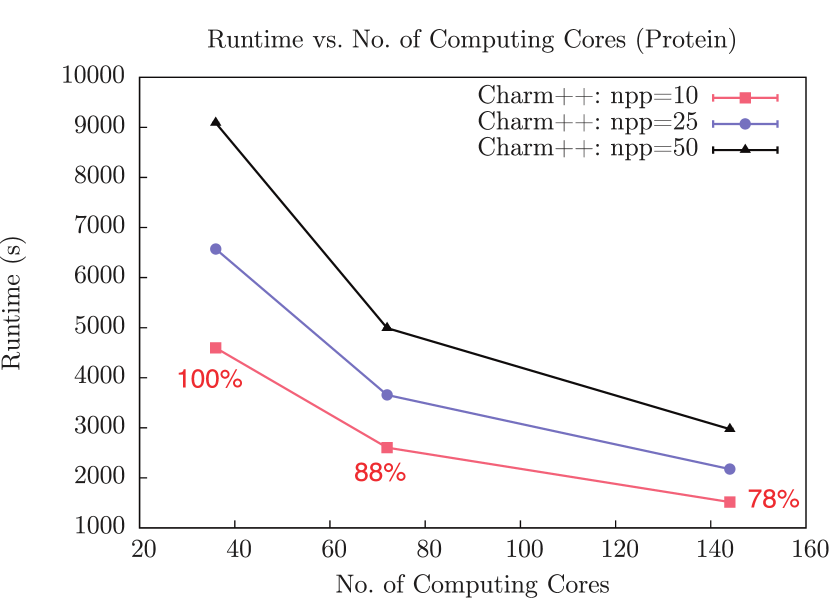
(a)

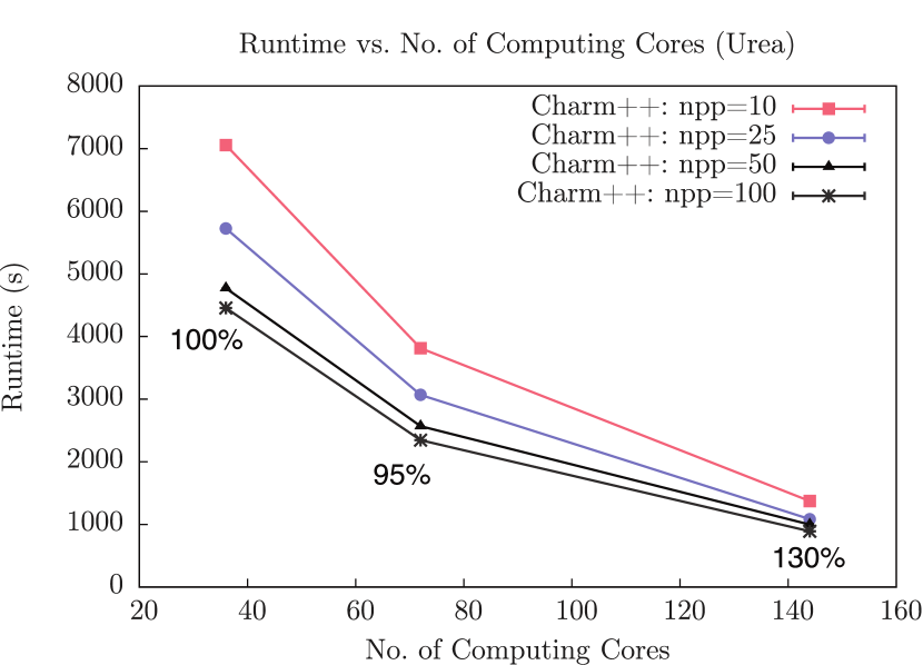
(b)

Figure 5: Runtimes of our Charm++ implementation for (a) a solvated protein (sparse) and (b) the molecular crystal urea (dense). As the number of partitions per processor is increased from 10 to 50 partitions per processor, runtimes for the protein system (a) increase, indicating over-decomposition beyond the optimal number of partitions, while runtimes for the more densely connected urea system (b) decrease. Parallel efficiency for the number of partitions with lowest runtimes are indicated; superlinear scaling is observed in the case of the urea simulation with 144 cores.

Fig. 5 shows the performance of our Charm++ implementation with block-partitioned subgraphs on distributed nodes for two systems with $\mathbf{P}$ of similar size: a solvated protein system (Fig. 5(a)), and a molecular crystal urea (Fig. 5(b)) that was previously considered in [10] and was chosen here because it has a more densely connected $\mathbf{P}$ compared to the solvated protein.

We observe that as the number of partitions per processor is varied (10, 25 and 50 partitions per processor), the runtime for the solvated protein in Fig. 5(a) increases, while the runtime for the crystal urea system decreases in Fig. 5(b). Given the same number of block-partitions, dense systems have more neighbors than sparse ones, so that denser systems lead to larger submatrices once neighbors are taken into account as halos. The size of submatrices determines data re-use (which mitigates communication costs), while the linear-algebraic cost scales cubically with submatrix size. Therefore, the optimal number of partitions balances communication and computational costs, and will vary with the system. In particular, comparing Figs. 5(a) and 5(b), we observe that with 10 partitions per processor, runtimes for the dense crystal urea system are considerably higher than for the sparse solvated protein system. Assuming communication costs have not dominated, this behavior is expected, as denser systems give rise to larger submatrices and higher computational costs for dense matrix multiplication. However, as the number of partitions is increased, submatrices of both physical systems get smaller; the sparse system is soon over-decomposed into more than the optimal number of partitions, while performance improves for the dense system, as there are still gains to be made by increasing the number of partitions.

Finally, the parallel efficiency was computed using [34]:

$$\text{parallel efficiency}=\frac{\text{speedup }}{\text{ratio of processors used}}=\frac{\left(\frac{t_{b}}{t_{n}}\right)}{\left(\frac{n}{b}\right)}\times 100\%,$$

where $t_{n}$ is the runtime for simulations using $n$ computing cores and $b=36$ is a baseline number against which the performance is compared (our implementation was tested for a minimum of 36 computing cores). Although we were unable to reach the strong scaling limit due to the number of computing cores available at the time, superlinear scaling is observed in the case of the crystal urea simulation with 144 cores. Superlinear scaling is uncommon but has been observed occasionally in applications [24, 19]. In particular, this behavior is to be expected when most or all of the working set (i.e., the amount of memory required for the process) can fit on the total available cache, and it is a known cause of superlinear scaling [17]. As the number of cores is increased, the parallel efficiency is expected to again fall below $100\%$.

3.2 Evaluation of G-SP2 with graph partitioning and the Charm++ runtime system

The G-SP2 algorithm in connection with both the blocking scheme and the METIS graph partitioning package were implemented using Charm++. SP2 computations were performed for the polyalanine 289 protein system previously studied in [10] as well as in previous sections of this paper. The computing cluster used for these computations was a Dell-built cluster running Linux with $14$ R730 computing nodes. All $14$ nodes were equipped with two $12$-core Intel Haswell CPUs, 64 GB of RAM ($22/3$ GB/core), a 200 GB solid state drive, gigabit ethernet, dual port FDR infiniband, and access to a shared $100+$ TB RAID storage system. Our implementation was built using Charm++ version $6.7.0$ and the RefineCommLB load balancer. This choice of the load balancer has been shown to yield robust performances on various inputs [29] and outperformed another popular choice, GreedyCommLB, in our experiments. Dense matrix-matrix multiplications were performed using the dgemm routine from mkl cblas (version $16.0.0$). All performance comparisons in this section are described in terms of the average overall runtime obtained from 10 independent calculations.

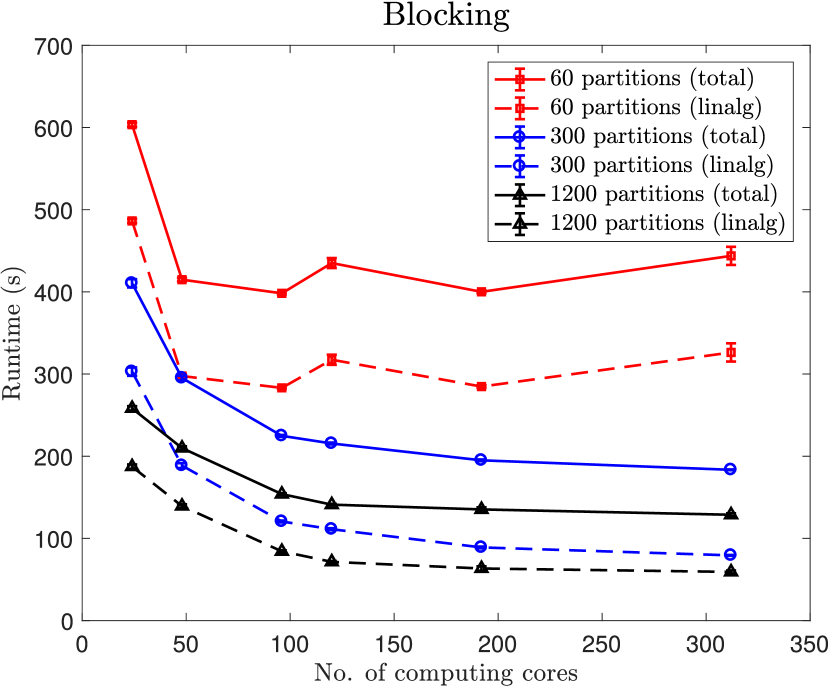
(c)

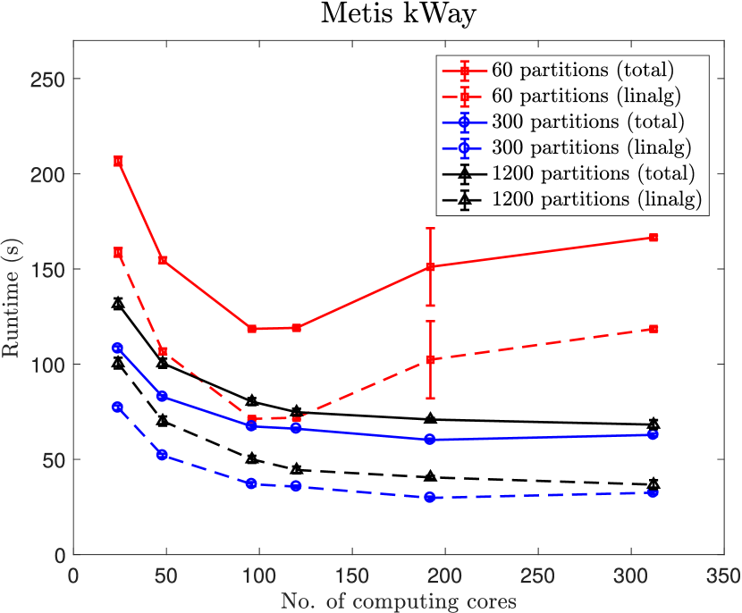
(d)

Figure 6: Runtime for density matrix calculations of the polyalanine 289 protein test system as a function of the number of processors. Subproblems obtained from $60$, $300$ and $1200$ partitions computed using (a) the block partitioning approach and (b) METIS. Runtimes for the total computation including communication costs are denoted by solid lines, and the times taken for linear algebra only are denoted by dotted lines.

Fig. 6 shows the total runtime taken to compute $\mathbf{P}$ for the polyalanine 289 protein system as the number of computing cores is varied. The graph was partitioned using a block partitioning approach (Fig. 6) as well as METIS (Fig. 6) into $60$, $300$ and $1200$ subproblems. First, a comparison of Figs. 6 and 6 demonstrates the advantage of using a tailored graph partitioning approach: Despite the additional effort for transforming the Hamiltonian into an undirected (and unweighted graph) and for partitioning it, using METIS yields a substantial two-fold decrease (or more) in total runtime compared to the block partitioning approach.

Figs. 6 and 6 also show the runtimes for independent SP2 subproblems if there were no overhead costs (i.e., the costs for linear algebra only). A significant fraction of the total runtime is indeed spent as overhead. A probable reason for the high overhead is that $\mathbf{H}$ and $\mathbf{P}$, as well as the associated connectivity graph, are initially processed serially so that all partitions were communicated from the mainChare node to all others. Compared to sequential SP2, where a large distributed matrix is communicated after every SP2 iteration, the communication overhead for G-SP2 is smaller because matrices are communicated only at the beginning and at the end of SP2 iterations. However, this cost is still significant and it is consistent with our findings in the previous section where the shared memory CnC application outperformed the Charm++ one.

4 Conclusions

This article presents a way to improve the performance of electronic structure calculations that rely on accurate density matrix calculations. Traditionally, the density matrix $\mathbf{P}$ is obtained through methods that scale as $O(N^{3})$, but methods such as the second-order spectral projection (SP2) scale linearly. Very recently, a graph-based approach to SP2 was developed (G-SP2) to divide the computation of $\mathbf{P}$ into independent data-parallel subproblems executed on distributed-memory machines, but at the expense of causing load imbalances. We explored task-based implementations of the G-SP2 algorithm using CnC and Charm++ asynchronous programming models. These implementations incorporate graph partitioning techniques developed in [26, 10] that are tailored for G-SP2. Task-based implementations of G-SP2 are important for mitigating load imbalances, especially if the same application is meant to be applied to different physical systems.

We expect the approach presented in this paper to scale well with the number of atoms due to the nearsightedness of physical systems. The nearsightedness limits the maximum subproblem size as every core vertex in any partition can only have a limited number of halo vertices or neighbors. Therefore, as the size of the system increases, the number of partitions can be increased in order to limit the maximum subproblem size until an optimal number of partitions is reached. In our experiments we also observed a significant communication overhead which, nevertheless, can be mitigated by constructing submatrices of $\mathbf{H}$ locally, and by using a parallel version of the METIS graph partitioning software. These are directions for future research.

We also investigate the effectiveness of different ways to generate subproblems. A simple locality based scheme can be advantageous in certain cases, but packages like METIS are more general and take distance into account indirectly. Blocking is a naïve way to obtain partitions and can be inferior to locality based submatrices because partitions obtained by blocking contain core vertices that are arranged according to their index in the Hamiltonian and not according to any relevant physical quantity. However, if blocking is exchanged for a more effective technique like METIS, the generation of subproblems becomes agnostic to how interactions between particular atoms vary with distance, and better subproblems (in terms of the computational cost metric used) are generated. Therefore, graph partitioning offers a general way to obtain subproblems based on the strength of interactions rather than distance between elements of $\mathbf{P}$. This feature is particularly useful for heterogenous systems with regions of dense and sparse connectivity.

To conclude, we found our Charm++ based G-SP2 implementation to be more suitable for QMD simulations of large systems than the CnC one as the former is readily extended to distributed-memory architectures. In addition to load balancing features, another advantage of using a mature runtime system such as Charm++ consists in the fact that further research in computer science to improve load balancing, fault tolerance or communication over large heterogenous clusters will directly carry over to our implementation without changes to the application code. Tuning Charm++ options to extract maximum performance from given hardware, expanding our tests to include large systems beyond 10,000 atoms, and a careful study of strong scaling limits for different physical systems could be future avenues for research.

Appendix A Details on the Evaluation of Runtime Systems

A.1 Charm++

Here we present the salient features of Charm++, followed by our Charm++ implementation of G-SP2. Additional details and a tutorial are available for Charm++ in [21].

1. Charm++ is an object-oriented programming framework that consists of migratable objects called chares. These objects are C++ objects, contain data and operations, of which some can be invoked from other chares via proxies. A Charm++ program starts with a main chare that interacts with the user, files, or other programs to obtain input data and instructions. The main chare then produces other chare workers that execute program tasks. Chares of the same type can be arranged in a collection called a chare array.

2. Charm++ tolerates latency by executing worker chares only when an execution call is received from another object and supports fault tolerance by automating checkpoints and restarts. Operations prescribed in a chare object are executed only when an execution call is received from another object (as in object-oriented programming) and when all data dependencies are satisfied. This is a useful mechanism for tolerating latency as a process is allocated to a processor only when a message for its execution is received. When using chare arrays, the same message can be broadcast to all the elements in the chare array at once. The runtime system then dynamically schedules and balances the processes to be run.

3. Both shared- and distributed-memory architectures can be targeted. Typically desired functionalities such as load balancing, memory management, detection of program initialization and termination, and hardware interfacing are available. The programmer can either choose to tune using various load-balancing schemes (or other functionalities) provided by Charm++ or can provide a self-defined scheme.

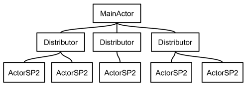
Figure 7: Roles of different chare objects constructed in Charm++ for the target G-SP2 application described in the main text.

Our Charm++ program uses three types of objects which we call MainActor, Distributors and ActorSP2. As shown in Fig. 7, the main chare called MainActor reads the Hamiltonian and other input parameters. It then sends the collected data to distributors that create their own chare arrays that receive and execute one SP2 subproblem. Computing nodes were assigned to distributors by round-robin scheme. Results from the individual SP2 subproblems are then sent to the MainActor which assembles the full density matrix $\mathbf{P}$.

For load balancing, we used the GreedyCommLB scheme of Charm++. Charm++ also includes MPI-interoperate functions, which can compile the above implementation as an ordinary library that can be called from standard MPI code. Our implementation of Charm++ also provides the option to compile the entire program as an MPI library that can been called from any MPI program using the advanced MPI-interoperate functions in Charm++.

A.2 Concurrent Collections CnC

With Charm++, an application is decomposed into migratable C++ objects that interact with each other through method calls (see section A.1). In contrast, CnC (Concurrent Collections) decomposes the application logic into a flow of data and control commands which, during execution, invoke various computations. Thus, CnC allows the programmer to focus on expressing the program at a higher level, while giving flexibility to the runtime system to schedule specific operations. We used the Intel CnC runtime system, which provides the programmer with a variety of scheduling options. The scheduler can also interact with the environment via flags or environment variables. The Intel CnC runtime system allows thread-sharing and may also spawn internal helper threads.

The salient features of the CnC programming model are summarized below. More detailed information can be found in [6, 5].

1. The dependency graph, also known as the CnC specification graph expresses the application logic with the help of objects and their tags: (a) step collections, which are operations to be executed; (b) data collections, which determine data flows; and (c) control collections, which act as switches that determine the order in which computations and data flow are allowed. Standard convention for representing these three different object types and their dependencies in the specification graph is with ellipses, rectangles, and hexagons, respectively. Collections are tracked by their respective tags.

2. The CnC philosophy holds that computations with dependencies can be scheduled concurrently. This is implemented by identifying computations that either produce or consume certain data, or ones that control or are controlled by another computation. While such an approach frees a wide range of possibilities to exploit parallelism, it also increases the complexity of the application since data, controls, and computations exist independently. As an aid to the programmer, templates for application-specific tuners are available, where the tuning expert can add additional soft constraints to guide the runtime.

3. Control and data flows must be explicitly defined in a CnC program via the API (the Application Program Interface which specifies how software components should interact with each other, typically through a set of routines and protocols). Because CnC assumes distributed-shared memory (i.e., it allows global variables), modifications to a shared data object must follow a control logic, making CnC deterministic [5].

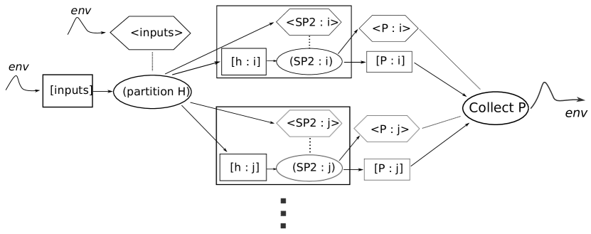
Figure 8: The specification graph for our CnC implementation of G-SP2.

In our G-SP2 implementation, we optimized the runtime for execution on a shared-memory machine. Thus, we accessed global variables and pointers within the steps, which in turn made the porting to a distributed-memory implementation more complicated. Our CnC specification graph is shown in Fig. 8. The environment provides input data as well as the control tag to initiate the program. The input data consists of both the Hamiltonian matrix and information to divide it into subproblems. The given Hamiltonian is then split into subproblems, which generates many instances of SP2 computations. Each SP2 computation, labeled by $i$, requires a partition of the Hamiltonian $[\text{h : i}]$, and a control prescription $<\text{SP2 : i}>$ and produces partitions of the density matrix $[\text{P : i}]$, which are then collected, and passed to the environment. During execution, input parameters are provided by the user or the environment. Each unique input set gives rise to an instance of the application, which is dynamically load balanced by the runtime system.

References

- Banerjee et al., [2016] Banerjee, A. S., Lin, L., Hu, W., Yang, C., and Pask, J. E. (2016). Chebyshev polynomial filtered subspace iteration in the discontinuous galerkin method for large-scale electronic structure calculations. Journal of Chemical Physics, 145(15):154101.
- Bock and Challacombe, [2013] Bock, N. and Challacombe, M. (2013). An optimized sparse approximate matrix multiply for matrices with decay. SIAM Journal on Scientific Computing, 35(1):C72–C98.
- Borštnik et al., [2014] Borštnik, U., VandeVondele, J., Weber, V., and Hutter, J. (2014). Sparse matrix multiplication: The distributed block-compressed sparse row library. Parallel Computing, 40(5):47–58.
- Bowler and Miyazaki, [2012] Bowler, D. and Miyazaki, T. (2012). Methods in electronic structure calculations. Reports on Progress in Physics, 75(3):036503.
- Budimlić et al., [2010] Budimlić, Z., Burke, M., Cavé, V., Knobe, K., Lowney, G., Newton, R., Palsberg, J., Peixotto, D., Sarkar, V., Schlimbach, F., and Taşırlar, S. (2010). Concurrent collections. Scientific Programming, 18(3-4):203–217.
- Burke et al., [2011] Burke, M. G., Knobe, K., Newton, R., and Sarkar, V. (2011). Concurrent collections programming model. In Encyclopedia of Parallel Computing, pages 364–371. Springer.
- Cawkwell and Niklasson, [2012] Cawkwell, M. and Niklasson, A. (2012). Energy conserving, linear scaling born-oppenheimer molecular dynamics. Journal of Chemical Physics, 137(13):134105.
- Cawkwell et al., [2012] Cawkwell, M., Sanville, E., Mniszewski, S., and Niklasson, A. (2012). Computing the density matrix in electronic structure theory on graphics processing units. Journal of Chemical Theory and Computation, 8(11):4094–4101.
- Cawkwell et al., [2014] Cawkwell, M. J., Wood, M. A., Niklasson, A., and Mniszewski, S. M. (2014). Computation of the density matrix in electronic structure theory in parallel on multiple graphics processing units. Journal of Chemical Theory and Computation, 10(12):5391–5396.
- Djidjev et al., [2016] Djidjev, H. N., Hahn, G., Mniszewski, S., Niklasson, A., and Sardeshmukh, V. B. (2016). Graph partitioning methods for fast parallel quantum molecular dynamics. SIAM Workshop on Combinatorial Scientific Computing (CSC16).
- Fattebert et al., [2016] Fattebert, J.-L., Osei-Kuffuor, D., Draeger, E. W., Ogitsu, T., and Krauss, W. D. (2016). Modeling dilute solutions using first-principles molecular dynamics: computing more than a million atoms with over a million cores. In Proceedings of the International Conference for High Performance Computing, Networking, Storage and Analysis, page 2. IEEE Press.
- Frenkel and Smit, [2001] Frenkel, D. and Smit, B. (2001). Understanding molecular simulation: from algorithms to applications, volume 1. Academic press.
- Genovese et al., [2008] Genovese, L., Neelov, A., Goedecker, S., Deutsch, T., Ghasemi, S. A., Willand, A., Caliste, D., Zilberberg, O., Rayson, M., Bergman, A., et al. (2008). Daubechies wavelets as a basis set for density functional pseudopotential calculations. Journal of Chemical Physics, 129(1):014109.
- Gerschgorin, [1931] Gerschgorin, S. (1931). Über die Abgrenzung der Eigenwerte einer Matrix. Izv. Akad. Nauk. USSR Otd. Fiz.-Mat. Nauk., 6:749–754.
- Goedecker, [1998] Goedecker, S. (1998). Decay properties of the finite-temperature density matrix in metals. Physical Review B, 58(7):3501.
- Goedecker, [1999] Goedecker, S. (1999). Linear scaling electronic structure methods. Reviews of Modern Physics, 71(4):1085.
- Gustafson, [1990] Gustafson, J. L. (1990). Fixed time, tiered memory, and superlinear speedup. In Proceedings of the Fifth Distributed Memory Computing Conference (DMCC5), pages 1255–1260.
- Haynes et al., [2006] Haynes, P. D., Mostof, A., Skylaris, C., and Payne, M. C. (2006). Onetep: linear-scaling density-functional theory with plane-waves. In Journal of Physics: Conference Series, volume 26, page 143. IOP Publishing.
- Hess et al., [2008] Hess, B., Kutzner, C., Van Der Spoel, D., and Lindahl, E. (2008). Gromacs 4: algorithms for highly efficient, load-balanced, and scalable molecular simulation. Journal of chemical theory and computation, 4(3):435–447.
- Ismail-Beigi and Arias, [1999] Ismail-Beigi, S. and Arias, T. (1999). Locality of the density matrix in metals, semiconductors, and insulators. Physical Review Letters, 82(10):2127.
- Kale et al., [2017] Kale, L. V., Pattabiraman, K., and Lee, C. W. (2017). Charm++ tutorial. website: http://charmplusplus.org/tutorial/.
- Karypis and Kumar, [1999] Karypis, G. and Kumar, V. (1999). A fast and high quality multilevel scheme for partitioning irregular graphs. SIAM Journal on Scientific Computing, 20(1):359–392.
- Karypis and Kumar, [2000] Karypis, G. and Kumar, V. (2000). Multilevel k-way hypergraph partitioning. VLSI Design, 11(3):285–300.
- Lange et al., [2013] Lange, M., Gorman, G., Weiland, M., Mitchell, L., and Southern, J. (2013). Achieving efficient strong scaling with petsc using hybrid mpi/openmp optimisation. In International Supercomputing Conference, pages 97–108. Springer.
- Mniszewski et al., [2015] Mniszewski, S., Cawkwell, M., Wall, M., Mohd-Yusof, J., Bock, N., Germann, T., and Niklasson, A. (2015). Efficient parallel linear scaling construction of the density matrix for born oppenheimer molecular dynamics. Journal of Chemical Theory and Computation, 11(10):4644–4654.
- Niklasson et al., [2016] Niklasson, A., Mniszewski, S. M., Negre, C. F., Cawkwell, M. J., Swart, P. J., Mohd-Yusof, J., Germann, T. C., Wall, M. E., Bock, N., and Djidjev, H. (2016). Graph-based linear scaling electronic structure theory. Journal of Chemical Physics, 144:234101.
- Niklasson et al., [2003] Niklasson, A., Tymczak, C., and Challacombe, M. (2003). Trace resetting density matrix purification in o(n) self-consistent-field theory. Journal of Chemical Physics, 118(19):8611–8620.
- Niklasson and Challacombe, [2004] Niklasson, A. M. and Challacombe, M. (2004). Density matrix perturbation theory. Physical Review Letters, 92(19):193001.
- Pilla et al., [2015] Pilla, L., Bozzetti, T., Castro, M., Navaux, P., and Méhaut, J.-F. (2015). ComprehensiveBench: a Benchmark for the Extensive Evaluation of Global Scheduling Algorithms. Journal of Physics: Conference Series, 649:1–12.
- Rubensson and Rudberg, [2014] Rubensson, E. H. and Rudberg, E. (2014). Chunks and Tasks: A programming model for parallelization of dynamic algorithms. Parallel Computing, 40(7):328–343.
- Sanders and Schulz, [2013] Sanders, P. and Schulz, C. (2013). Think Locally, Act Globally: Highly Balanced Graph Partitioning. In Proceedings of the 12th International Symposium on Experimental Algorithms (SEA’13), volume 7933 of LNCS, pages 164–175. Springer.
- Sanville et al., [2010] Sanville, E., Bock, N., Coe, J., Martinez, E., Mniszewski, S., Negre, C., Niklasson, A., and Cawkwell, M. (2010). Los alamos transferable tight-binding for energetics (latte) los alamos national laboratory.
- Sena et al., [2011] Sena, A. M., Miyazaki, T., and Bowler, D. R. (2011). Linear scaling constrained density functional theory in conquest. Journal of Chemical Theory and Computation, 7(4):884–889.
- Xavier and Iyengar, [1998] Xavier, C. and Iyengar, S. S. (1998). Introduction to parallel algorithms, volume 1, chapter 1. John Wiley & Sons.
- Zhou et al., [2006] Zhou, Y., Saad, Y., Tiago, M. L., and Chelikowsky, J. R. (2006). Self-consistent-field calculations using chebyshev-filtered subspace iteration. Journal of Computational Physics, 219(1):172–184.