Adaptive Estimation of Noise Variance and Matrix Estimation via USVT Algorithm

Abstract.

We propose a method for estimating the entries of a large noisy matrix when the variance of the noise, $\sigma^{2}$, is unknown without putting any assumption on the rank of the matrix. We consider the estimator for $\sigma$ introduced by Gavish and Donoho [13] and give an upper bound on its mean squared error. Then with the estimate of the variance, we use a modified version of the Universal Singular Value Thresholding (USVT) algorithm introduced by Chatterjee [10] to estimate the noisy matrix. Finally, we give an upper bound on the mean squared error of the estimated matrix.

1. Introduction

Consider the statistical estimation problem where the unknown parameters of interest are the entries of a $m\times n$ matrix $M$, where $m\leq n$. Suppose we have observed the $m\times n$ matrix $X$, a noisy version of $M$, that is $X=M+\sigma A$. The entries of $A$ are i.i.d. with mean zero and variance one and $\sigma$ is an unknown positive constant. The goal is to recover $M$ from this noisy observation $X$ and give an upper bound on the mean squared error (MSE) of its estimate. Given an estimator $\hat{M}$ for $M$, the $\text{MSE}(\hat{M})$ is defined as

$$\text{MSE}(\hat{M}):=\mathbb{E}\Big{[}\frac{1}{mn}\sum_{i=1}^{m}\sum_{j=1}^{n}(m_{ij}-\hat{m}_{ij})^{2}\Big{]},$$ (1)

where $m_{ij}$ and $\hat{m}_{ij}$ are respectively the $(i,j)$th entries of the matrices $M$ and $\hat{M}$.

The problem of estimating the entries of a large matrix from noisy and/or incomplete observations has been studied widely. A common approach for solving this problem is to assume that $M$ is a low-rank matrix. Under the low-rank assumption there is a huge body of work using spectral methods, such as [2, 1, 16, 17, 13, 21]. Some other works under certain model assumptions are [12, 24].

In a different direction, Emmanuel Candès and his collaborators [6, 5, 9, 8] studied this problem by penalizing the nuclear norm of the matrix under convex constraints. Some other notable examples of this penalization approach are [11, 18, 19, 22, 23].

In 2015, Chatterjee [10] proposed a simple estimation procedure, the USVT algorithm. In that work, Chatterjee considered the problem of matrix estimation without putting any assumption on the rank of the matrix $M$. However, in [10] he assumed that the noise entries and therefore the entries of $X$ lie in a bounded interval. Although he added that the results should stay valid when the entries of $X-M$ are $N(0,\sigma^{2})$ when $\sigma$ is known, but the problem of estimating $M$ when $\sigma$ is unknown, remained unsolved.

Later, in [13] Gavish and Donoho proposed an estimator for $\sigma$ based on the observed matrix $X$. In that work, using the Marčhenko-Pastur law, they construct their estimator as a function of the median singular value of matrix $X$. They showed that this estimate almost surely converges to $\sigma$ as $n$ goes to infinity under this assumption that the additive noise is orthogonally invariant. In a different work, Nadler and Kritchman [20], proposed an iterative algorithm for estimating the unknown $\sigma$.

In this paper, we consider the problem of matrix estimation when the variance of the noise, $\sigma$, is unknown. We do not put any assumption on the rank of the matrix or boundedness of its entries. However, we consider the mild assumption that entries of the noise matrix $A$ are i.i.d. and sub-Gaussian. First, we give an upper bound on the mean squared error of the estimator of $\sigma$ from [13], $\hat{\sigma}$. Using the estimate of $\sigma$, we modify the USVT algorithm [10] and give an estimate of $M$, $\hat{M}$, based on the observed matrix $X$. At last we give an upper bound on the mean squared error of $\hat{M}$.

In section 2 we study the estimator of the variance. Theorem 2.2 gives an upper bound on the mean squared error of this estimate. Then we give an estimator of $M$ and in Theorem 2.3 give an upper bound on the mean squared error of this estimator of $M$. In section 3 we study a simulated example. Proofs of all theorems and lemmas are in section 4.

2. Set up and Main Results

Consider the $m\times n$ random matrix $X=[x_{ij}]$. Without loss of generality, we let $m\leq n$. Let $X$ be a noisy version of $M$, $X=M+\sigma A$, where $M=[m_{ij}]$ is a deterministic unknown matrix and $A=[\epsilon_{ij}]$ is a random matrix with i.i.d. entries independent of $M$ and $\mathbb{E}[\epsilon_{ij}]=0$ and $\mathbb{E}[\epsilon_{ij}^{2}]=1$. Noise level $\sigma>0$ is an unknown deterministic constant. The final goal is to estimate the entries of $M=[m_{ij}]\in\mathbb{R}^{m\times n}$.

Let’s assume that $\sigma$ is known and $|\epsilon_{ij}|\leq 1$, then following the steps of USVT algorithm [10] bellow, we find $\hat{M}$ an estimate of $M$.

1. Let $\sum_{i=1}^{m}\lambda_{i}(X)u_{i}v_{i}^{T}$ be the singular value decomposition of $X$, where $\lambda_{1}(X)\geq\ldots\geq\lambda_{m}(X)$ are the singular values of $X$ and $u_{i}$ and $v_{i}$ are its left and right singular vectors.

2. Choose a small positive number $\eta\in(0,1]$ and let $S$ be the set of “thresholded singular values”,

   $$S_{\sigma}:=\{i:\lambda_{i}(X)\geq(2+\eta)\sigma\sqrt{n}\}.$$

3. Define $\hat{M}:=\sum_{i\in S_{\sigma}}\lambda_{i}(X)u_{i}v_{i}^{T}$.

Note that set $S_{\sigma}$ depends on $\sigma$ and also uses the earlier assumption on boundedness of $\epsilon_{ij}$’s.

To continue, first we introduce some notations and definitions.

2.1. Definitions and Notation

Let $X=[x_{ij}]$ be $m\times n$, where $m\leq n$, a random matrix with $x_{ij}$’s i.i.d. and $\mathbb{E}[x_{ij}]=0$ and $\mathbb{E}[x_{ij}^{2}]=1$. Let

$$Y_{n}=\frac{1}{n}XX^{T},$$

and let $\lambda_{1}(Y_{n})\geq\cdots\geq\lambda_{m}(Y_{n})$ be the singular values of $Y_{n}$. Define $\mu_{m}$ as a random counting measure,

$$\mu_{m}(A)=\frac{1}{m}\#\left\{\lambda_{j}(Y_{n})\in A\right\},\quad A\subset\mathbb{R}.$$

Marčhenko-Pastur Law: Let $m,\,n\,\to\,\infty$ such that $m/n\,\to\,\gamma\in(0,1)$ . Then $\mu_{m}\,\to\,\mu_{\text{MP}}^{\gamma}$ in distribution, where

$$d\mu_{\text{MP}}^{\gamma}(x)={\frac{1}{2\pi}}{\frac{\sqrt{(\gamma_{+}-x)(x-\gamma_{-})}}{\gamma x}}\,\mathbf{1}_{[\gamma_{-},\gamma_{+}]}\,dx$$

with $\gamma_{\pm}=(1\pm{\sqrt{\gamma}})^{2}$.

Let $\mathbb{F}_{\gamma}(x)$ and $\mathbb{F}_{n}$ be the cumulative distribution function (cdf) of $\mu_{\text{MP}}^{\gamma}$ and $\mu_{m}$ respectively

$$\mathbb{F}_{\gamma}(x)=\int_{\gamma_{-}}^{x}d\mu_{\text{MP}}^{\gamma}(t),\qquad\mathbb{F}_{n}(x)=\int_{0}^{x}\,d\mu_{m}(t).$$

Definition 2.1.

For the $m\times n$ matrix $X$ consider the singular value decomposition $X=U\Sigma V^{T}$, where $\Sigma$ is a $m\times n$ diagonal matrix with diagonal entries $\lambda_{1}(X)\geq\cdots\geq\lambda_{m}(X)\geq 0$, and $U$ and $V$ are unitary matrices of size $m\times m$ and $n\times n$ respectively. The nuclear norm of $X$ is defined as the sum of its singular values,

$$\|X\|_{*}:=\sum_{i=1}^{m}\lambda_{i}(X).$$

2.2. Estimation of $\sigma$

We consider the following estimator of $\sigma$ that was proposed by Donoho and Gavish [13],

$$\hat{\sigma}(X)=\frac{\text{med}(\lambda_{i}(X))}{\sqrt{n\mu_{\gamma}}},$$

where $\text{med}(\lambda_{i}(X))$ is the median of $\lambda_{i}(X)$’s and

$$\mu_{\gamma}=\mathbb{F}_{\gamma}^{-1}(\frac{1}{2}).$$ (2)

In [13], Donoho and Gavish have shown that

$$\lim_{n\rightarrow\infty}\hat{\sigma}(X)=\sigma\qquad\text{a.s.}$$

They have made this conclusion under an asymptotic frame work in which they have assumed that the distribution of $A$ is orthogonally invariant, meaning that for $R_{1}$ and $R_{2}$, $m\times m$ and $n\times n$ orthogonal matrices, $A$ and $R_{1}AR_{2}$ have the same distribution. We consider this estimator without the extra invariance assumption on the noise distribution. Theorem 2.2 provides an upper bound on the MSE of $\hat{\sigma}(X)$.

Theorem 2.2.

Let $X=[x_{ij}]$ be a $m\times n$ random matrix with $x_{ij}$’s distributed i.i.d. from a sub-Gaussian distribution such that $\mathbb{E}(x_{ij})=m_{ij}$ and $Var(x_{ij})=\sigma^{2}$ for unknown values of $\sigma$ and $m_{ij}$’s. For

$$\hat{\sigma}=\frac{\emph{\text{med}}(\lambda_{i}(X))}{\sqrt{n\mu_{\gamma}}},$$

we have

$$\mathbb{E}\Big{[}(\hat{\sigma}-\sigma)^{2}\Big{]} \leq \frac{2\|M\|_{*}^{2}}{\mu_{\gamma}n^{2}}+\frac{\sigma^{2}C_{\gamma}}{\mu_{\gamma}n}+\frac{\sigma^{2}C_{\gamma,\epsilon}}{\mu_{\gamma}n^{1-\epsilon}},$$

where $C_{\gamma,\epsilon}$ and $C_{\gamma}$ are non-negative constants independent of $n$ and $\sigma$.

If $\|M\|_{*}=o(n)$, Theorem 2.2 implies that the $\text{MSE}(\hat{\sigma})$

In [20] Kritchman and Nadler suggested an iterative method for estimating the $\sigma$. The strength of $\hat{\sigma}$ for us is that it’s easy to compute. Also its simple definition made it possible to use random matrix theory to give the upper bound on its MSE.

2.3. Modified USVT estimator of $M$

With $\hat{\sigma}$ as the estimator of $\sigma$, we use the following modified version of the USVT algorithm to find an estimator for $M$.

1. Let $\sum_{i=1}^{m}\lambda_{i}(X)u_{i}v_{i}^{T}$ be the singular value decomposition of $X$, where $\lambda_{1}(X)\geq\ldots\geq\lambda_{m}(X)$ are the singular values of $X$ and $u_{i}$ and $v_{i}$ are the left and right singular vectors.

2. Choose a small positive number $\eta\in(0,1]$ and let $S$ be the set of “thresholded singular values”

   $$S_{\hat{\sigma}}=\{i:\lambda_{i}(X)\geq(2+\eta)\hat{\sigma}\sqrt{n}\}.$$

3. Define $\hat{M}=\sum_{i\in S_{\hat{\sigma}}}\lambda_{i}(X)u_{i}v_{i}^{T}$.

Theorem 2.3 gives an upper bound on the MSE of $\hat{M}$.

Theorem 2.3.

Let $X=[x_{ij}]$ be a $m\times n$ random matrix with $x_{ij}$’s distributed i.i.d. from a sub-Gaussian distribution such that $\mathbb{E}(x_{ij})=m_{ij}$ and $Var(x_{ij})=\sigma^{2}$ for unknown values of $\sigma$ and $m_{ij}$’s. Let

$$\hat{\sigma}=\frac{\emph{\text{med}}(\lambda_{i}(X))}{\sqrt{n\mu_{\gamma}}},$$

and for $\eta\in(0,1)$ define $\hat{M}$ using the modified USVT algorithm. Then

$$\emph{\text{MSE}}(\hat{M})=\mathbb{E}\big{[}\frac{1}{mn}\|\hat{M}-M\|_{F}^{2}\big{]}$$

$$\leq \frac{C_{0}\sigma\|M\|_{*}}{\gamma n\sqrt{n}}+(2+\eta)^{2}\sigma^{2}\left(C_{1}+C_{2}\frac{\|M\|_{*}^{4}}{\sigma^{4}\mu_{\gamma}^{2}n^{4}}\right)^{1/2}\max\{\sqrt{\frac{C_{\epsilon,\gamma}\sigma}{\mu_{\gamma}\eta^{2}n^{1-\epsilon}}},\sqrt{\frac{\|M\|_{*}^{2}}{n^{2}\sigma^{2}\eta^{2}\mu_{\gamma}}}\},$$

where $C_{0},C_{1}$, and $C_{2}$ are constants, and $C_{\epsilon,\gamma}$ is a constant that depends on $\epsilon$ and $\gamma$.

The upper bounds depend on the $\|M\|_{*}$ and $\sigma$, the unknown parameters of the model, and the parameter of choice $\eta$. Theorem 2.3 implies that if $\|M\|_{*}=o(n)$ then $\emph{\text{MSE}}(\hat{M})$ is of order of $\sigma^{2}$.

3. Simulation

In this section we consider a simple simulated example. Let $n=1000$ and $m=200$ and we consider the sequence $\lambda_{1}\geq\cdots\geq\lambda_{200}$ where $\lambda_{i}=\exp(3-i/50)$ for $i\in\{1,\cdots,200\}$. Then for each $r\in\{50,100,150,200\}$ we define the following signal matrix

$$M_{r}=UD_{r}V^{T}$$

where $D_{r}$ is a $m\times n$ rectangular diagonal matrix with the $i$-th diagonal entry equal to $\lambda_{i}\mathds{1}\{i\leq r\}$, and $U$ and $V$ are randomly uniform orthogonal matrices of size $m\times m$ and $n\times n$ respectively. For each choice of $r\in\{50,100,150,200\}$, we generated 100, independent noise matrix $A$ with $N(0,1)$ i.i.d. entries and considered observed matrix $X=M_{r}+\sigma A$ for different values of $\sigma$. In Figure 1 we have plotted the mean squared error of $\hat{\sigma}$ and $\hat{M_{r}}$ for different values of $r$ and $\sigma$. We have set $\eta=0.02$ in the USVT algorithm.

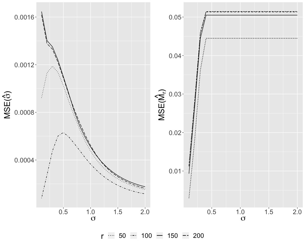
Figure 1. Estimated mean squared error of $\hat{\sigma}$ and $\hat{M}$ for different values of rank, $r=50,100,150$, and $200$. The our error bounds in Theorems 2.2 and 2.3 do not depend on the rank, but it depends on the nuclear norm of the mean matrix $M_{r}$. In this example we have $\|M_{50}\|_{*}=641.193$, $\|M_{100}\|_{*}=877.0753$, $\|M_{150}\|_{*}=963.851$, and $\|M_{200}\|_{*}=995.775$.

4. Proofs

In what follows $c$, $C$ and $C_{i}$ for $i\in\mathbb{N}$ are non-negative constants independent of the parameters of the problem, and $C_{\gamma}$ and $C_{\epsilon,\gamma}$ are non-negative constants that only depends on $\epsilon$ and pair of $\epsilon$ and $\gamma$ respectively. For simplicity these values may change from line to line or even in a line. For simplicity in notation and without loss of generality we assume that $m$ is an even number and therefore use $\lambda_{m/2}$ instead of $\text{med}(\lambda_{i})$ for the median singular value.

4.1. Proofs of Theorems 2.2 and 2.3

4.1.1. Proof of Theorem 2.2

Proof.

By adding and subtracting $\lambda_{m/2}(X-M)$ and inequality $(a+b)^{2}\leq 2a^{2}+2b^{2}$ we have

$$\mathbb{E}\Big{[}\Big{(}\hat{\sigma}-\sigma\Big{)}^{2}\Big{]} = \mathbb{E}\Big{[}\Big{(}\frac{\lambda_{m/2}(X)}{\sqrt{n\mu_{\gamma}}}-\sigma\Big{)}^{2}\Big{]}$$ (3)

$$\leq \frac{2}{n\mu_{\gamma}}\mathbb{E}\Big{[}\Big{(}\lambda_{m/2}(X)-\lambda_{m/2}(X-M)\Big{)}^{2}\Big{]}$$

$$+ \frac{2\sigma^{2}}{n\mu_{\gamma}}\mathbb{E}\Big{[}\Big{(}\lambda_{m/2}(\frac{X-M}{\sigma})-\sqrt{n\mu_{\gamma}}\Big{)}^{2}\Big{]}.$$ (4)

Using Lemma 4.2 for (4) we have,

$$\frac{2\sigma^{2}}{n\mu_{\gamma}}\mathbb{E}\Big{[}\Big{(}\lambda_{m/2}(\frac{X-M}{\sigma})-\sqrt{n\mu_{\gamma}}\Big{)}^{2}\Big{]} = \frac{2\sigma^{2}}{\mu_{\gamma}}\mathbb{E}\Big{[}\Big{(}\lambda_{m/2}(\frac{A}{\sqrt{n}})-\sqrt{\mu_{\gamma}}\Big{)}^{2}\Big{]}$$ (5)

$$= \frac{2\sigma^{2}}{\mu_{\gamma}}\mathbb{E}\Big{[}\Big{(}\sqrt{\mathbb{F}_{n}^{-1}(\frac{1}{2})}-\sqrt{\mathbb{F}_{\gamma}^{-1}(\frac{1}{2})}\Big{)}^{2}\Big{]}$$

$$\leq \frac{\sigma^{2}C_{\epsilon,\gamma}}{\mu_{\gamma}n^{1-\epsilon}}.$$

To give an upper bound on (3), we use the following inequality from [4] (page 75). For any two $n\times n$ matrices $A_{1}$ and $A_{2}$ and any two indices $i$ and $j$ such that $i+j\leq n+1$,

$$\lambda_{i+j-1}(A_{1}+A_{2})\leq\lambda_{i}(A_{1})+\lambda_{j}(A_{2}).$$ (6)

For matrices $X-M$ and $M$, $0<k\leq\lfloor\sqrt{n}\rfloor$, and indices $m/2-k$ and $k+1$, (6) gives

$$\lambda_{m/2}(X) \leq \lambda_{m/2-k}(X-M)+\lambda_{k+1}(M),$$ (7)

and for matrices $X$ and $M$, and indices $m/2$ and $k+1$, (6) gives

$$\lambda_{m/2+k}(X-M) \leq \lambda_{m/2}(X)+\lambda_{k+1}(M).$$ (8)

Subtracting $\lambda_{m/2}(X-M)$ from the left and right sides of (7) and (8) gives

$$\lambda_{m/2}(X)-\lambda_{m/2}(X-M) \leq \lambda_{m/2-k}(X-M)-\lambda_{m/2}(X-M)+\lambda_{k+1}(M),$$

$$\lambda_{m/2}(X)-\lambda_{m/2}(X-M) \geq \lambda_{m/2+k}(X-M)-\lambda_{m/2}(X-M)-\lambda_{k+1}(M).$$

Therefore

$$(\lambda_{m/2}(X)-\lambda_{m/2}(X-M))^{2}$$ (9)

$$\leq 2\max\{(\lambda_{m/2-k}(X-M)-\lambda_{m/2}(X-M))^{2},(\lambda_{m/2+k}(X-M)-\lambda_{m/2}(X-M))^{2}\}$$

$$+ 2\lambda_{k+1}(M)^{2}$$

Note that

$$\lambda_{k+1}(M)\leq\frac{\|M\|_{*}}{k+1}.$$ (10)

Taking expectation of (9) and inequality (10) gives

$$\mathbb{E}[(\lambda_{m/2}(X)-\lambda_{m/2}(X-M))^{2}]$$ (11)

$$\leq 2\mathbb{E}[(\lambda_{m/2-k}(X-M)-\lambda_{m/2}(X-M))^{2}]$$

$$+ 2\mathbb{E}[(\lambda_{m/2+k}(X-M)-\lambda_{m/2}(X-M))^{2}]$$

$$+ 2(\frac{\|M\|_{*}}{k+1})^{2}.$$

To give an upper bound on (11) we use the following decomposition

$$\lambda_{m/2-k}(X-M)-\lambda_{m/2}(X-M) = \sigma\sqrt{n}(\sqrt{\mathbb{F}_{n}^{-1}(\frac{1}{2}-\frac{k}{n})}-\sqrt{\mathbb{F}_{n}^{-1}(\frac{1}{2})})$$ (13)

$$= \sigma\sqrt{n}\left[\sqrt{\mathbb{F}_{n}^{-1}(\frac{1}{2}-\frac{k}{n})}-\sqrt{\mathbb{F}_{\gamma}^{-1}(\frac{1}{2}-\frac{k}{n})}\right]+$$

$$\sigma\sqrt{n}\left[\sqrt{\mathbb{F}_{\gamma}^{-1}(\frac{1}{2})}-\sqrt{\mathbb{F}_{n}^{-1}(\frac{1}{2})}\right]+$$

$$\sigma\sqrt{n}\left[\sqrt{\mathbb{F}_{\gamma}^{-1}(\frac{1}{2}-\frac{k}{n})}-\sqrt{\mathbb{F}_{\gamma}^{-1}(\frac{1}{2})}\right].$$

Using inequality $(a+b)^{2}\leq 2a^{2}+2b^{2}$, and Lemma 4.2 we have

$$\mathbb{E}[(\lambda_{m/2-k}(X-M)-\lambda_{m/2}(X-M))^{2}]\leq$$ (14)

$$4\sigma^{2}n\mathbb{E}\left[\left(\sqrt{\mathbb{F}_{n}^{-1}(\frac{1}{2}-\frac{k}{n})}-\sqrt{\mathbb{F}_{\gamma}^{-1}(\frac{1}{2}-\frac{k}{n})}\right)^{2}\right]+$$

$$4\sigma^{2}n\mathbb{E}\left[\left(\sqrt{\mathbb{F}_{\gamma}^{-1}(\frac{1}{2})}-\sqrt{\mathbb{F}_{n}^{-1}(\frac{1}{2})}\right)^{2}\right]+$$

$$2\sigma^{2}n\left[\sqrt{\mathbb{F}_{\gamma}^{-1}(\frac{1}{2}-\frac{k}{n})}-\sqrt{\mathbb{F}_{\gamma}^{-1}(\frac{1}{2})}\right]^{2}$$

$$\leq 2\sigma^{2}C_{\epsilon,\gamma}n^{\epsilon}+2\sigma^{2}n\left[\sqrt{\mathbb{F}_{\gamma}^{-1}(\frac{1}{2}-\frac{k}{n})}-\sqrt{\mathbb{F}_{\gamma}^{-1}(\frac{1}{2})}\right]^{2}.$$

Similary

$$\mathbb{E}[(\lambda_{m/2+k}(X-M)-\lambda_{m/2}(X-M))^{2}]\leq$$ (15)

$$4\sigma^{2}n\mathbb{E}\left[\left(\sqrt{\mathbb{F}_{n}^{-1}(\frac{1}{2}+\frac{k}{n})}-\sqrt{\mathbb{F}_{\gamma}^{-1}(\frac{1}{2}+\frac{k}{n})}\right)^{2}\right]+$$

$$4\sigma^{2}n\mathbb{E}\left[\left(\sqrt{\mathbb{F}_{\gamma}^{-1}(\frac{1}{2})}-\sqrt{\mathbb{F}_{n}^{-1}(\frac{1}{2})}\right)^{2}\right]+$$

$$2\sigma^{2}n\left[\sqrt{\mathbb{F}_{\gamma}^{-1}(\frac{1}{2}+\frac{k}{n})}-\sqrt{\mathbb{F}_{\gamma}^{-1}(\frac{1}{2})}\right]^{2}$$

$$\leq 2\sigma^{2}C_{\epsilon,\gamma}n^{\epsilon}+2\sigma^{2}n\left[\sqrt{\mathbb{F}_{\gamma}^{-1}(\frac{1}{2}+\frac{k}{n})}-\sqrt{\mathbb{F}_{\gamma}^{-1}(\frac{1}{2})}\right]^{2}.$$

Using the mean value theorem, we find the following bound on (14), and (15).

$$|\sqrt{\mathbb{F}_{\gamma}^{-1}(\frac{1}{2}\pm\frac{k}{n})}-\sqrt{\mathbb{F}_{\gamma}^{-1}(\frac{1}{2})}| \leq C_{\gamma}|\mathbb{F}_{\gamma}^{-1}(\frac{1}{2}\pm\frac{k}{n})-\mathbb{F}_{\gamma}^{-1}(\frac{1}{2})|$$ (16)

$$\leq \frac{C_{\gamma}}{\sqrt{n}}.$$

Putting (14), and (15) together with (16) gives

$$\mathbb{E}[(\lambda_{m/2}(X)-\lambda_{m/2}(X-M))^{2}]\leq\sigma^{2}C_{\epsilon,\gamma}n^{\epsilon}+\sigma^{2}C_{\gamma}.$$ (17)

Inequalities (17), and (10) with $k=\lfloor\sqrt{n}\rfloor$ completes the proof,

$$\mathbb{E}\Big{[}(\hat{\sigma}-\sigma)^{2}\Big{]} \leq \frac{2\|M\|_{*}^{2}}{\mu_{\gamma}n^{2}}+\frac{\sigma^{2}C_{\gamma}}{\mu_{\gamma}n}+\frac{\sigma^{2}C_{\gamma,\epsilon}}{\mu_{\gamma}n^{1-\epsilon}}.$$

∎

4.2. Proof of Theorem 2.3

Proof.

Consider the following two sets $E_{1}$ and $E_{2}$,

$$E_{1} = \{\|X-M\|\leq(2+\frac{\eta}{2})\sigma\sqrt{n}\},$$

$$E_{2} = \{|\hat{\sigma}-\sigma|\leq\frac{\eta}{20}\sigma\}.$$

Consider the following decomposition,

$$\mathbb{E}\|\hat{M}-M\|_{F}^{2}=\mathbb{E}[\|\hat{M}-M\|_{F}^{2}\mathds{1}\{(E_{1}\cap E_{2})^{\mathsf{c}}\}]+\mathbb{E}[\|\hat{M}-M\|_{F}^{2}\mathds{1}\{(E_{1}\cap E_{2})\}].$$

Using Lemma 4.1 from [10], which we copy without its proof, we find an upper bound on $\mathbb{E}[\|\hat{M}-M\|_{F}^{2}\mathds{1}\{(E_{1}\cap E_{2})\}]$.

Lemma 4.1.

Let $D=\sum_{i=1}^{m}\sigma_{i}u_{i}v_{i}^{T}$ be the singular value decomposition of $D$. Fix any $\delta>0$ and define

$$\hat{B}\coloneqq\sum_{i:\sigma_{i}>(1+\delta)\|D-B\|}\sigma_{i}x_{i}y_{i}^{T}.$$

Then

$$\|\hat{B}-B\|_{F}\leq K(\delta)(\|D-B\|\|B\|_{*})^{1/2},$$

where $K(\delta)=(4+2\delta)\sqrt{2/\delta}+\sqrt{2+\delta}$.

For $\delta\geq\eta/5$, we have $K(\delta)\leq C\sqrt{1+\delta}$. On the set $E_{1}\bigcap E_{2}$, we have $\delta\geq\eta/5$. Thus by using Lemma 4.1 we have,

$$\|\hat{M}-M\|_{F}^{2} \leq C(1+\delta)\|X-M\|\|M\|_{*}$$

$$\leq C\sqrt{n}\sigma\|M\|_{*}.$$

Therefore

$$\mathbb{E}[\|\hat{M}-M\|_{F}^{2}\mathds{1}\{(E_{1}\cap E_{2})\}]\leq C\sqrt{n}\sigma\|M\|_{*}.$$

Then by Cauchy-Schwartz inequality we get

$$\mathbb{E}[\|\hat{M}-M\|_{F}^{2}\mathds{1}\{(E_{1}\cap E_{2})^{\mathsf{c}}\}]\leq\sqrt{\mathbb{E}[\|\hat{M}-M\|_{F}^{4}]\mathbb{E}[(E_{1}\cap E_{2})^{\mathsf{c}}]}.$$ (18)

Note that

$$\mathbb{P}[(E_{1}\cap E_{2})^{\mathsf{c}}]\leq\mathbb{P}(E_{1}^{\mathsf{c}})+\mathbb{P}(E_{2}^{\mathsf{c}}).$$

By Proposition 2.4 in [26]

$$\mathbb{P}(E_{1}^{\mathsf{c}})\leq Ce^{-c\eta^{2}n},$$ (19)

and by Chebyshev’s inequality

$$\mathbb{P}(E_{2}^{\mathsf{c}}) \leq \frac{800\|M\|_{*}^{2}}{\mu_{\gamma}\sigma^{2}\eta^{2}n^{2}}+\frac{400C_{\gamma}}{\mu_{\gamma}\eta^{2}n}+\frac{400C_{\gamma,\epsilon}}{\mu_{\gamma}\eta^{2}n^{1-\epsilon}}.$$ (20)

Inequalities (19) and (20) together give

$$\mathbb{P}[(E_{1}\cap E_{2})^{\mathsf{c}}]\leq Ce^{-c\eta^{2}n}+\frac{800\|M\|_{*}^{2}}{\mu_{\gamma}\sigma^{2}\eta^{2}n^{2}}+\frac{C_{\gamma,\epsilon}}{\mu_{\gamma}\eta^{2}n^{1-\epsilon}}.$$ (21)

To finish finding a bound on (18), we find an upper bound on $\mathbb{E}[\|\hat{M}-M\|^{4}_{F}]$. Using inequality $(a+b)^{2}\leq 2a^{2}+2b^{2}$, we have

$$\|\hat{M}-M\|_{F}^{4} = (\sum_{ij}(m_{ij}-\hat{m}_{ij})^{2})^{2}$$

$$= (\sum_{ij}(m_{ij}-x_{ij}+x_{ij}-\hat{m}_{ij})^{2})^{2}$$

$$\leq (2\sum_{ij}(m_{ij}-x_{ij})^{2}+(x_{ij}-\hat{m}_{ij})^{2})^{2}$$

$$= 4(\sum_{ij}(m_{ij}-x_{ij})^{2}+\sum_{ij}(x_{ij}-\hat{m}_{ij})^{2})^{2}$$

$$\leq 8(\sum_{ij}(m_{ij}-x_{ij})^{2})^{2}+8(\sum_{ij}(x_{ij}-\hat{m}_{ij})^{2})^{2}$$

$$= 8\|M-X\|_{F}^{4}+8\|X-\hat{M}\|_{F}^{4}.$$

Note that

$$\|\hat{M}-X\|_{F}^{4} = \|\sum_{\lambda_{i}(X)<(2+\eta)\hat{\sigma}\sqrt{n}}\lambda_{i}(X)u_{i}v_{i}^{T}\|_{F}^{4}$$

$$= (\|\sum_{\lambda_{i}(X)<(2+\eta)\hat{\sigma}\sqrt{n}}\lambda_{i}(X)u_{i}v_{i}^{T}\|_{F}^{2})^{2}$$

$$\leq n^{4}(2+\eta)^{4}{\hat{\sigma}}^{4}.$$

Therefore

$$\mathbb{E}[\|\hat{M}-X\|_{F}^{4}] \leq n^{4}(2+\eta)^{4}\mathbb{E}[{\hat{\sigma}}^{4}],$$ (22)

and Lemma 4.3 gives

$$\mathbb{E}[\|\hat{M}-X\|_{F}^{4}] \leq 4n^{4}(2+\eta)^{4}(4\sigma^{4}+\frac{C_{\epsilon,\gamma}\sigma^{4}}{n^{2-\epsilon}}+\frac{64\|M\|_{*}^{4}}{n^{4}\mu_{\gamma}^{2}})$$ (23)

Now note that

$$\|X-M\|_{F}^{4} = \sum_{i,j}(x_{ij}-m_{ij})^{4}+\sum_{(i,j)\neq(l,k)}(x_{ij}-m_{ij})^{2}(x_{lk}-m_{lk})^{2}$$

Since $x_{ij}$’s are i.i.d sub-Gaussian random variables and thus their forth moment is bounded,

$$\mathbb{E}[\|X-M\|_{F}^{4}] \leq C\gamma^{2}\sigma^{4}n^{4}.$$ (24)

Inequalities (24) and (22) and Lemma 4.3 give

$$\mathbb{E}\|\hat{M}-M\|_{F}^{2}\leq C_{0}\sqrt{n}\sigma\|M\|_{*}+$$

$$\left(4n^{4}(2+\eta)^{4}(C_{1}\sigma^{4}+\frac{C_{\epsilon,\gamma}\sigma^{4}}{n^{2-\epsilon}}+\frac{64\|M\|_{*}^{4}}{n^{4}\mu_{\gamma}^{2}})\right)^{1/2}\times\left(C_{2}e^{-c\eta^{2}n}+\frac{800\|M\|_{*}^{2}}{\mu_{\gamma}\sigma^{2}\eta^{2}n^{2}}+\frac{C_{\gamma,\epsilon}}{\mu_{\gamma}\eta^{2}n^{1-\epsilon}}\right)^{1/2}.$$

This completes the proof of Theorem 2.3,

$$\text{MSE}(\hat{M})=\frac{1}{\gamma n^{2}}\mathbb{E}[\|\hat{M}-M\|_{F}^{2}]\leq$$

$$\frac{C_{0}\sigma\|M\|_{*}}{\gamma n\sqrt{n}}+(2+\eta)^{2}\sigma^{2}\left(C_{1}+C_{2}\frac{\|M\|_{*}^{4}}{\sigma^{4}\mu_{\gamma}^{2}n^{4}}\right)^{1/2}\left(\frac{C_{\epsilon,\gamma}\sigma}{\mu_{\gamma}\eta^{2}n^{1-\epsilon}}+\frac{\|M\|_{*}^{2}}{n^{2}\sigma^{2}\eta^{2}\mu_{\gamma}}\right)^{1/2}\leq$$

$$\frac{C_{0}\sigma\|M\|_{*}}{\gamma n\sqrt{n}}+\sqrt{2}(2+\eta)^{2}\sigma^{2}\left(C_{1}+C_{2}\frac{\|M\|_{*}^{4}}{\sigma^{4}\mu_{\gamma}^{2}n^{4}}\right)^{1/2}\max\{\sqrt{\frac{C_{\epsilon,\gamma}\sigma}{\mu_{\gamma}\eta^{2}n^{1-\epsilon}}},\sqrt{\frac{\|M\|_{*}^{2}}{n^{2}\sigma^{2}\eta^{2}\mu_{\gamma}}}\}.$$

∎

4.3. Proofs of the lemmas

Lemma 4.2.

For any $\epsilon>0$ and $k\in\{0,1,\ldots,\lfloor\sqrt{n}\rfloor\}$ almost surely

$$|\sqrt{\mathbb{F}_{n}^{-1}(\frac{1}{2}+\frac{k}{n})}-\sqrt{\mathbb{F}_{\gamma}^{-1}(\frac{1}{2}+\frac{k}{n})}|\leq C_{\epsilon,\gamma}n^{-1/2+\epsilon},$$ (25)

where $C_{\epsilon,\gamma}$ is a constant that only depends on $\gamma$ and $\epsilon$.

Proof.

Let

$$\Delta_{n,\gamma}^{*}:=\sup_{x}|\mathbb{F}_{n}(x)-\mathbb{F}_{\gamma}(x)|.$$

In [14], Götze and Tikhomirov have shown that for any $\epsilon>0$, the rate of almost sure convergence of $\Delta_{n,\gamma}^{*}$ is at most $O(n^{-1/2+\epsilon})$. This means that there exist a constant $C_{\epsilon}$ such that $\Delta_{n,\gamma}^{*}\leq C_{\epsilon}n^{-1/2+\epsilon}$ almost surely.

For $t=\mathbb{F}_{\gamma}^{-1}(\frac{1}{2}+\frac{k}{n})$ and $\delta>0$ such that $[t-\delta,t+\delta]\subset(\gamma_{-},\gamma_{+})$ we have

$$\mathbb{F}_{\gamma}(t+\delta)-\mathbb{F}_{\gamma}(t-\delta) = \int_{t-\delta}^{t+\delta}d\mu_{MP}^{\gamma}(x)$$

$$= \frac{1}{2\gamma\pi}\int_{t-\delta}^{t+\delta}\frac{\sqrt{(\gamma_{+}-x)(x-\gamma_{-})}}{x}dx$$

$$\leq C_{\gamma}\int_{t-\delta}^{t+\delta}\frac{1}{x}dx$$

$$= -C_{\gamma}\log(1-\frac{2\delta}{t+\delta})$$

$$= C_{\gamma}\delta.$$

Note that

$$|\mathbb{F}_{n}(\mathbb{F}_{n}^{-1}(\frac{1}{2}+\frac{k}{n}))-\mathbb{F}_{\gamma}(\mathbb{F}_{n}^{-1}(\frac{1}{2}+\frac{k}{n}))|\leq\Delta_{n,\gamma}^{*}\leq C_{\epsilon}n^{-1/2+\epsilon},$$ (26)

where the second inequality is almost sure. Now if $|\mathbb{F}_{n}^{-1}(\frac{1}{2}+\frac{k}{n})-\mathbb{F}_{\gamma}^{-1}(\frac{1}{2}+\frac{k}{n})|\geq\delta$ then we have

$$|\mathbb{F}_{\gamma}(\mathbb{F}_{n}^{-1}(\frac{1}{2}+\frac{k}{n}))-\mathbb{F}_{\gamma}(\mathbb{F}_{\gamma}^{-1}(\frac{1}{2}+\frac{k}{n}))|\geq C_{\gamma}\delta$$ (27)

and this is possible only for $\delta\leq C_{\epsilon}n^{-1/2+\epsilon}$. Therefore

$$|\mathbb{F}_{n}^{-1}(\frac{1}{2}+\frac{k}{n})-\mathbb{F}_{\gamma}^{-1}(\frac{1}{2}+\frac{k}{n})|\leq C_{\epsilon,\gamma}n^{-1/2+\epsilon}$$ (28)

almost surely. Using the mean value theorem for function $f(x)=\sqrt{x}$ we have

$$|\sqrt{\mathbb{F}_{n}^{-1}(\frac{1}{2}+\frac{k}{n})}-\sqrt{\mathbb{F}_{\gamma}^{-1}(\frac{1}{2}+\frac{k}{n})}|\leq C_{\epsilon,\gamma}n^{-1/2+\epsilon}.$$ (29)

∎

Lemma 4.3.

Let $X=[x_{ij}]$ be a $m\times n$ random matrix with $x_{ij}$’s distributed i.i.d. from a sub-Gaussian distribution such that $\mathbb{E}(x_{ij})=m_{ij}$ and $Var(x_{ij})=\sigma^{2}$ for some unknown value of $\sigma$. For any arbitrary $\epsilon>0$ and

$$\hat{\sigma}=\frac{\emph{\text{med}}(\lambda_{i}(X))}{\sqrt{n\mu_{\gamma}}},$$

we have

$$\mathbb{E}[\hat{\sigma}^{4}]\leq 4\sigma^{4}+\frac{C_{\epsilon,\gamma}\sigma^{4}}{n^{2-\epsilon}}+\frac{64\|M\|_{*}^{4}}{n^{4}\mu_{\gamma}^{2}},$$

where $C_{\epsilon,\gamma}>0$ is a constant independent of $n$ and $\sigma$.

Proof.

Using inequality $(a+b)^{2}\leq 2a^{2}+2b^{2}$ we write

$$\mathbb{E}[\hat{\sigma}^{4}] \leq 8\mathbb{E}[(\hat{\sigma}-\sigma)^{4}]+8\sigma^{4}.$$

By adding and subtracting $\lambda_{m/2}(X-M)$ we have

$$\mathbb{E}[(\hat{\sigma}-\sigma)^{4}] \leq \frac{8}{n^{2}\mu_{\gamma}^{2}}\mathbb{E}[(\lambda_{m/2}(X)-\lambda_{m/2}(X-M))^{4}]$$

$$+ \frac{8\sigma^{4}}{n^{2}\mu_{\gamma}^{2}}\mathbb{E}[(\lambda_{m/2}(\frac{X-M}{\sigma})-\sqrt{n\mu_{\gamma}})^{4}].$$

Note that by Lemma 4.2

$$\frac{8\sigma^{4}}{n^{2}\mu_{\gamma}^{2}}\mathbb{E}\left[\left(\lambda_{m/2}(\frac{X-M}{\sigma})-\sqrt{n\mu_{\gamma}}\right)^{4}\right] = \frac{8\sigma^{4}}{\mu_{\gamma}^{2}}\mathbb{E}\left[\left(\sqrt{\mathbb{F}_{n}^{-1}(\frac{1}{2})}-\sqrt{\mathbb{F}_{\gamma}^{-1}(\frac{1}{2})}\right)^{4}\right]$$ (30)

$$\leq \frac{\sigma^{4}C_{\epsilon,\gamma}}{\mu_{\gamma}^{2}n^{2-\epsilon}}.$$

Using decomposition (13) we have

$$\mathbb{E}\left[(\lambda_{m/2}(X)-\lambda_{m/2}(X-M))^{4}\right]$$

$$\leq 512n^{2}\sigma^{4}\mathbb{E}\left[\left(\sqrt{\mathbb{F}_{n}^{-1}(\frac{1}{2}-\frac{k}{n})}-\sqrt{\mathbb{F}_{\gamma}^{-1}(\frac{1}{2}-\frac{k}{n})}\right)^{4}\right]$$

$$+ 512n^{2}\sigma^{4}\mathbb{E}\left[\left(\sqrt{\mathbb{F}_{n}^{-1}(\frac{1}{2}+\frac{k}{n})}-\sqrt{\mathbb{F}_{\gamma}^{-1}(\frac{1}{2}+\frac{k}{n})}\right)^{4}\right]$$

$$+ 1028n^{2}\sigma^{4}\mathbb{E}\left[\left(\sqrt{\mathbb{F}_{n}^{-1}(\frac{1}{2})}-\sqrt{\mathbb{F}_{\gamma}^{-1}(\frac{1}{2})}\right)^{4}\right]$$

$$+ 64n^{2}\sigma^{4}\left[\sqrt{\mathbb{F}_{\gamma}^{-1}(\frac{1}{2}+\frac{k}{n})}-\sqrt{\mathbb{F}_{\gamma}^{-1}(\frac{1}{2})}\right]^{4}$$

$$+ 64n^{2}\sigma^{4}\left[\sqrt{\mathbb{F}_{\gamma}^{-1}(\frac{1}{2}-\frac{k}{n})}-\sqrt{\mathbb{F}_{\gamma}^{-1}(\frac{1}{2})}\right]^{4}$$

$$+ 8(\frac{\|M\|_{*}}{k+1})^{4}.$$

Then Lemma 4.2 gives

$$\mathbb{E}\left[(\lambda_{m/2}(\frac{X}{\sigma})-\lambda_{m/2}(\frac{X-M}{\sigma}))^{4}\right] \leq C_{\epsilon,\gamma}n^{\epsilon}\sigma^{4}+C_{\gamma}\sigma^{4}+8(\frac{\|M\|_{*}}{k+1})^{4}.$$ (31)

Therefore (31), and (30) with $k=\lfloor\sqrt{n}\rfloor$ completes the proof,

$$\mathbb{E}[(\hat{\sigma}-\sigma)^{4}] \leq \frac{C_{\epsilon,\gamma}\sigma^{4}}{n^{2-\epsilon}}+\frac{C_{\epsilon,\gamma}\sigma^{4}}{n^{2-\epsilon}\mu_{\gamma}^{2}}+\frac{C_{\gamma}\sigma^{4}}{n^{2}\mu_{\gamma}^{2}}+\frac{64\|M\|_{*}^{4}}{n^{4}\mu_{\gamma}^{2}}$$ (32)

$$\leq \frac{C_{\epsilon,\gamma}\sigma^{4}}{n^{2-\epsilon}}+\frac{64\|M\|_{*}^{4}}{n^{4}\mu_{\gamma}^{2}}.$$

∎

References

• Achlioptas, D. [2007] Achlioptas, D. and McSherry, F.(2007) Fast Computation of Low-rank Matrix Approximations. J. ACM., 54, no.2, Art. 9, 19pp.MR 2295993
• Azar, Y. [2001] Azar, Y. Flat, A. Karlin, A. McSherry, F. and Sala, J.(2001) Spectral Analysis of Data. Proceedings of the Thirty-third Annual ACM symposium on Theory of Computing, 619–626.
• Bai, Z. D. [1993] Bai, Z. D.(1993) Convergence Rate of Expected Spectral Distributions of Large Random Matrices. Part I. Wigner Matrices. J. ACM.,21, no.2, 625–648.MR 1217560
• Bhatia, R. [1997] Bhatia, R.(1997) Matrix analysis. Graduate Texts in Mathematics, 169. Springer-Verlag, New York, MR 1477662
• CandΓ¨s, E. J. [2010] Candes, E. and Plan, Y.(2010) Matrix Completion With Noise. Ann. Statist., 98, no.6, 925–936.
• CandΓ¨s, E. J. [2009] CandΓ¨s, E. J. and Recht, B.(2009) Exact Matrix Completion Via Convex Optimization. Found. Comput. Math., 9, no.6, 717–772.MR 2565240
• CandΓ¨s, E. J. [2006] CandΓ¨s, E. J. Romberg, J. and Tao, T.(2006) Robust Uncertainty Principles: Exact Signal Reconstruction From Highly Incomplete Frequency Information. IEEE Trans. Inform. Theory., 52, no.2, 489–509.MR 2236170
• CandΓ¨s, E. J. [2010] Cai, J. and CandΓ¨s, E. J. and Shen, Z.(2010) A Singular Value Thresholding Algorithm For Matrix Completion. SIAM J. Optim., 20, no.4, 1956–1982.MR 2600248
• CandΓ¨s, E. J. [2010] CandΓ¨s, E. J. and Tao, T.(2010) The Power of Convex Relaxation: Near Optimal Matrix Completion. IEEE Trans. Inform. Theory., 56, no.5, 12053–2080.MR 2723472
• Chatterjee, S. [2015] Chatterjee, S.(2015) Matrix Estimation By Universal Singular Value Thresholding. Ann. Statist., 43, no.1, 177–214.MR 3285604
• Donoho, D. [2014] Donoho, D. and Gavish, M.(2014) Minimax Risk of Matrix Denoising By Singular Value Thresholding. Ann. Statist., 42,no.6, 2413–2440.MR 3269984
• Fazel, M. [2002] Fazel, M.(2002) Matrix Rank Minimization With Applications. Ph.D. thesis, Stanford University
• Gavish, M. [2014] Gavish, M. and Donoho, D. L.(2014) The Optimal Hard Threshold For Singular Values Is $4/\sqrt{3}$. IEEE Trans. Inform. Theory., 60, no.8, 5040–5053.
• Gotze, F. [2004] Gotze, F. and Tikhomirov, A.(2004) Rate of convergence in probability to the Marčhenko-Pastur law. Bernoulli., 10, no.3, 503–548 MR 2061442
• Gotze, F. [2014] Gotze, F. and Tikhomirov, A.(2014) On the Rate of Convergence to the Marčhenko-Pastur Distribution. arXiv:1110.1284v3
• Keshavan, R. H. [2010] Keshavan, R. H. Montanari, A. Oh, S.(2010) Matrix Completion From Noisy Entries. J. Mach. Learn. Res., 11, 2057–2078.MR 2678022
• Keshavan, R. H. [2010] Keshavan, R. H. Montanari, A. Oh, S.(2010) Matrix Completion From a Few Entries. IEEE Trans. Inform. Theory., 56, no.6, 2980–2998.MR 2683452
• Koltchinskii, V. [2011] Koltchinskii, V.(2011) Von Neumann Entropy Penalization And Low-rank Matrix Estimation. Ann. Statist., 39, no.6, 2936–2973.MR 3012397
• Koltchinskii, V. [2011] Koltchinskii, V. Lounici, K. and Tsybakov, A. B.(2011) Nuclear-norm Penalization And Optimal Rates For Noisy Low-rank Matrix Completion. Ann. Statist., 39, no.5, 2302–2329.MR 2906869
• Kritchman, S. [2009] Kritchman, S. and Nadler, B.(2009) Non-parametric Detection of The Number of Signals: Hypothesis Testing And Random Matrix Theory. IEEE Trans. Signal Process., 57,no.10, 3930–3941.MR 2683143
• Mazumder, R. [2010] Mazumder, R. Hastie, T. and Tibshirani, R.(2010) Spectral Regularization Algorithms For Learning Large Incomplete Matrices. J. Mach. Learn. Res., 11, 2287–2322.MR 2719857
• Negahban, S. [2011] Negahban, S. and Wainwright, M. J.(2011) Estimation of (near) Low-rank Matrices With Noise And High-dimensional Scaling. Ann. Statist., 11,no.2, 1069–1097.MR 2816348
• Rennie, J.D. [2005] Rennie, J.D. and Srebro, N.(2005) Fast Maximum Margin Factorization For Collaborative Prediction. ICML ’05 Proceedings of the 22nd international conference on Machine learning, 713–719.
• Rohde, A. [2011] Rohde, A. and Tsybakov, A. B.(2011) Estimation of High-dimensional Low-rank Matrices. Ann. Statist., 39,no.2, 887–930.MR 2816342
• Rudelson, M. [2007] Rudelson, M. and Vershynin, R.(2007) Sampling From Large Matrices: An Approach Through Geometric Functional Analysis. J. ACM., 54,no.4, Art. 21, 19pp.MR 2351844
• Rudelson, M. [2010] Rudelson, M. and Vershynin, R.(2010) Non-asymptotic Theory of Random Matrices: Extreme Singular Values. Proceedings of the International Congress of Mathematicians. Volume III, Hindustan Book Agency, New Delhi 1576–1602.MR 2827856