An Optimized Information-Preserving Relational Database Watermarking Scheme for Ownership Protection of Medical Data

Abstract

Recently, a significant amount of interest has been developed in motivating physicians to use e-health technology (especially Electronic Medical Records (EMR) systems). An important utility of such EMR systems is: a next generation of Clinical Decision Support Systems (CDSS) will extract knowledge from these electronic medical records to enable physicians to do accurate and effective diagnosis. It is anticipated that in future such medical records will be shared through cloud among different physicians to improve the quality of health care. Therefore, right protection of medical records is important to protect their ownership once they are shared with third parties. Watermarking is a proven well known technique to achieve this objective. The challenges associated with watermarking of EMR systems are: (1) some fields in EMR are more relevant in the diagnosis process; as a result, small variations in them could change the diagnosis, and (2) a misdiagnosis might not only result in a life threatening scenario but also might lead to significant costs of the treatment for the patients. The major contribution of this paper is an information-preserving watermarking scheme to address the above-mentioned challenges. We model the watermarking process as a constrained optimization problem. We demonstrate, through experiments, that our scheme not only preserves the diagnosis accuracy but is also resilient to well known attacks for corrupting the watermark. Last but not least, we also compare our scheme with a well known threshold-based scheme to evaluate relative merits of a classifier. Our pilot studies reveal that – using proposed information-preserving scheme – the overall classification accuracy is never degraded by more than 1%. In comparison, the diagnosis accuracy, using the threshold-based technique, is degraded by more than 18% in a worst case scenario.

I Introduction

Pervasive and ubiquitous deployment of information and communication technology infrastructure is bringing a revolution the way health care services are provided. Consequently, e-health technology and its associated systems are being actively standardized, adopted and deployed. An important component of modern e-health technology is EMR systems in which a patient’s medical history, his vitals, lab tests, and diagnostic images are stored [1]. In the health reform package, Obama administration is offering between $44,000 and $64,000 to the physicians who would use EMR systems. The incentive amount for adopting EMR systems at a hospital is $11 million [2].

In order to provide quality care, it is relevant that the access to medical records be provided in a ubiquitous fashion to the concerned physicians. Therefore, the inter-operable EMR systems are becoming the top priority in the US [3]. This demands exchanging and sharing sensitive health records in a network cloud. Moreover, next generation of CDSSs will have the ability to extract knowledge from the electronic medical records and use them to assist physicians in making accurate and effective diagnosis. In such scenarios, the shared data might be illegally sold to third parties by an unauthorized party. In order to cater for such a situation, the data needs to be right protected so that an unauthorized party might be sued in a court of law. This is only possible, if the data owner is able to prove that the illegally sold data is his property. Therefore, it is important to not only protect the privacy of the patients [4], [5], [6] but also the ownership (copyright) of the medical data shared with collaborative partners or third party vendors. In a recent survey, it is reported that frauds related to stolen medical records have risen from 3$\%$ in 2008 to $7\%$ in 2009 (approximately a $112$% increase) [7]. Similarly, confidential medical records of patients in the EMR of a prestigious private hospital in UK were illegally sold to undercover investigators for $4\pounds$ per record [8]. It is stated that theft of medical records is more serious because it takes more than twice the time to detect a fraud related to the medical information and the average cost is $12,100 which is more than twice the cost for other types of data theft [9]. A recent case related to an illegal sale of the medical data is reported in [10]. Therefore, it is important that medical records be right protected in a manner where ownership could unambiguously be determined. (The data theft is becoming a serious issue even for the most reliable brands like LexisNexis, Polo Ralph Lauren, HSBC, NCR, and a number of renowned universities [11]).

In this paper, we propose a novel right protection scheme that will establish the ownership of EMR data, and consequently, will make its illegal sale very difficult (even if the intruder has altered the original data). Recently, some watermarking techniques are proposed for databases [12], [13], [14] but they are unable to address a significant challenge related to EMR: insertion of a watermark must not result in changing health and medical history of a patient to a level where a decision maker (or system) can misdiagnose the patient. If a patient is misdiagnosed, it might not only put his life on risk but also result in significantly enhancing the cost of health care. In order to address this problem, we propose the concept of information-preserving watermarking. The basic motivation behind this technique is to first develop a model that determines the correlation of different features with the diagnosis. We model the process of computing a suitable watermark as a constrained optimization problem [15]. Once the watermark is computed, it is inserted (with $O(n)$ complexity) by utilizing the knowledge of correlation of those features that have negligible impact on the diagnosis. As a result, the diagnosis rules are preserved and it is important because these rules are used for diagnosing the patients and suggesting a relevant treatment plan. Consequently, if a rule is changed due to insertion of watermark then the suggested treatment would also change which may cause serious harm to the life of a patient. Moreover, wrong treatment will also waste time and money of the patients. Therefore, it is mandatory that during watermarking of EMR, diagnosis rules must be preserved. Moreover, the inserted watermark should be imperceptible to intruders and they should not be able to corrupt it by launching malicious attacks [15], [16]. Last but not least, multiple insertions of the same watermark should not corrupt medical records.

Recent research proves that computational intelligence techniques, especially Particle Swarm Optimization (PSO) [17], [18], are ideally suited for solving constrained optimization problems in realtime. In this paper, we use PSO to create an optimized watermark that – once inserted into an EMR – does not alter the diagnosis rules. The major contributions of our work are: (1) an intelligent information-preserving watermarking technique for EMR systems that ensures data usability constraints and also preserves the rules after the watermark encoding, (2) realtime insertion of watermark into an EMR system, and (3) a robust watermark decoding scheme that is resilient against all kinds of malicious attacks.

The rest of the paper is organized as follows. In the next section, we provide a brief overview of the research related to our work by emphasizing the different direction of our work. In section III, we discuss our proposed scheme followed by experiments and results in section IV. Finally, we conclude the paper with an outlook to our future research.

II Related Work

Agrawal et al. [15] proposed the idea of watermarking using least significant bits (LSB). They do not account for multibit watermarks which makes their technique vulnerable against simple attacks, for example shifting of only one least significant bit results in loss of watermark. Xinchun et al. have proposed a watermarking scheme for relational databases that uses weights (assigned by users) of attributes to identify the location where the watermark is to be inserted [19]. They intuitively argue that the primary key of a database is the most important attribute and hence a watermark should not be inserted in it. They, however, did not consider the importance of ranking attributes because their focus was not on using a database for data mining and decision support systems.

Sion et al. [13] presented a watermarking scheme in which data is partitioned using marker tuples. But if an attacker launches an attack on marker tuples, the synchronization is lost. The marker tuples decide the boundaries for the partitions but successful insertion or deletion attacks on marker tuples would result in synchronization errors. Li et al. [20] have proposed a watermarking technique to detect and localize alterations made to a database relation with relevant attributes. Li et al. have proposed a technique for fingerprinting relational data [21] by extending the technique proposed in [15]. Jiang et al. proposed an invisible watermarking technique using Discrete Wavelet Transform (DWT) in [22].

A well known problem with all these techniques is: they are not resilient to malicious attacks launched by an intruder. Recently, Shehab et al. have proposed a robust watermarking scheme in [14]. They model a bit encoding algorithm as an optimization problem and use Genetic Algorithm (GA) [23] and Pattern Search (PS) [24] to do the optimization. They use a threshold based approach coupled with a majority vote to decode the watermark. The focus of their work is to show that their scheme is robust to malicious attacks (insertion and deletion) launched by an intruder. In [25] Bertino et al. have proposed a technique for preserving the ownership of outsourced medical data but they their focus was on preserving the classification potential and the diagnostic rules.

In comparison, the focus of our work is to rank attributes (features) on the basis of their importance in a decision making process. Our objective is to identify weak attributes by developing a knowledge model that correlates the effect of an attribute on the decision making process. The major difference of our approach from previous techniques is that we first identify the classification potential of each attribute for a given diagnosis. Furthermore, we use the knowledge of classification potential for every candidate attribute to calculate the watermark which ensures that the data usability constraints remain intact and also the diagnosis rules are preserved. As a result, we meet the most important requirement while right protecting an EMR: to preserve the diagnostic semantics of the health record of a patient (i.e. a patient should not be misdiagnosed).

The proposed technique uses an optimization technique to first create a watermark which ensures that data usability constraints are not violated. Once the watermark is created, we embed it in realtime into an EMR system. In comparison, other techniques [14] use optimization techniques during watermark embedding and hence they take a significant amount of time. As a consequence, they are not suitable for realtime insertion of watermark into an EMR system.

Moreover, our technique is also robust to malicious attacks because it does not target any specific group of tuples for watermarking (almost all other techniques developed so far use a secret key to select some group of tuples as candidate attribute(s) for watermarking).

III The Proposed Information-Preserving Watermarking Technique

We propose a framework that does information-preserving right protection of EMR systems (see Figure 1). The framework operates in two modes: (1) Watermark encoding, and (2) Watermark decoding. In the watermark encoding phase, the objective is to determine a watermark that, once inserted into an $EMR$, does not alter the vital features to an extent that the patient is misdiagnosed. Similarly, the objective of the decoding phase is to accurately detect a watermark in an efficient manner. We now discuss the watermark encoding scheme in the following.

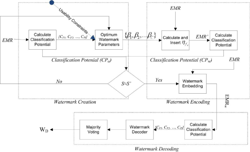
Figure 1: The architecture of the proposed scheme.

III-A Watermark Encoding Phase

In this phase (or mode), three important steps are to be performed: (1) quantifying the importance of a patient’s vitals (or history information) and their correlation with the diagnosis, (2) computing a set of possible values to calculate the watermark and then selecting the optimum one with the help of an optimization scheme, and (3) embedding the information-preserving optimum watermark into EMR fields for right protection.

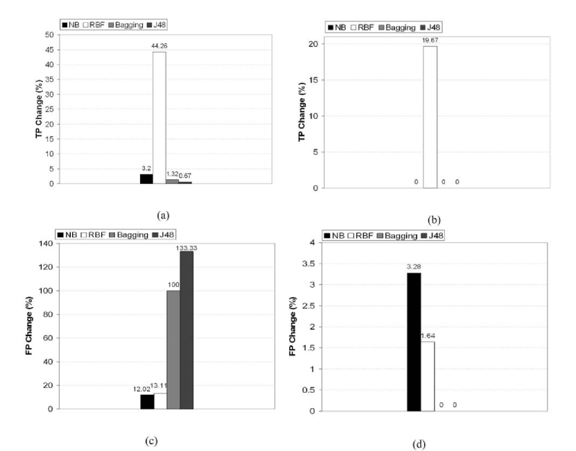
Figure 2: Effect of inserting a watermark, using techniques that do not preserve information, in attributes with different $C_{P}$ on various classification statistics for diagnosing hypertension in the hypertension dataset. (a) Change in TP(%) when only one attribute with the highest $C_{P}$ is watermarked. (b) Change in TP(%) when only one attribute with the lowest $C_{P}$ is watermarked. (c) Change in FP(%) when only one attribute with the highest $C_{P}$ is watermarked. (d) Change in FP(%) when only one attribute with the lowest $C_{P}$ is watermarked.

For a quick reference, Table I lists the notations used in this paper. (We recommend that a reader should refer to this table whenever he/she is in doubt about the interpretation of an encountered symbol.)

TABLE I: Notations used in the paper.

Symbol	Description	Symbol	Description
$EMR$	Original database	$b$	The watermark bit
$EMR_{W}$	Watermarked database	$\mu$	The mean of an attribute
R	Total number of rows in a table (or dataset)	$r$	A row in the database table
$F$	The features set present in a table (or dataset)	$\sigma$	The standard deviation of an attribute $a$
$TP$	The number of positive instances correctly detected	$min(a)$	The minimum value of an attribute $a$
	as positive
$FP$	The number of negative instances incorrectly detected	$\varrho$	The change in the value of an attribute in $EMR_{W}$
	as positive		after an attack
$TN$	The number of negative instances correctly detected	$max(a)$	The maximum value of an attribute $a$
	as negative
$FN$	The number of positive instances incorrectly detected	$C$	The cardinality of $f$
	as negative
$C_{P}$	Classification potential of a feature in the database	$\hbar$	Usability constraints matrix
$\Delta_{C_{P}}$	Change in classification potential of a feature in the	$\eta_{f_{c}}$	The exact value of watermark for a feature $f_{c}$
	database after changing its value		row of the database relation
$C_{S}$	Overall classification statistics of the database	$\Delta$	A matrix containing secret parameters
$C_{P_{O}}$	The classification potential of a feature in $EMR$	$\tau$	The watermark decoder used for watermark decoding
$C_{P_{W}}$	The classification potential of a feature in $EMR_{W}$	$\gamma$	A correction factor to adjust value of $\tau$
$a$	An attribute or column in the original database ($EMR$)	$EMR^{{}^{\prime}}_{W}$	A watermarked database after the malicious attacks
$x_{a}$	The value of an attribute $a$	$l$	The length of the watermark
$IG(R,a)$	The information gain of an attribute $a$ in the database	$\eta_{d_{f_{c}}}$	Detected amount of change in the value of a feature after
			an attack on the watermark bit b
$H(R)$	The entropy of $R$ rows	$\eta_{\Delta_{f_{c}}}$	The difference between the changes detected in the value
			of a feature during the encoding and decoding process
$P$	The probability of a certain event	$W$	Embedded watermark
$f_{c_{W}}$	The watermarked candidate feature $f_{c}$	$W_{D}$	Decoded watermark
$A$	Total number of attributes in the database	$EMR_{W_{P}}$	$EMR$ watermarked by the proposed scheme
$m$	The number of features selected for watermarking	$EMR_{W_{s}}$	$EMR$ watermarked by Shehab’s scheme
$\beta_{f_{c}(min)}$	Lower bound (percentage) for the watermark value for	$\Delta_{P}$	The percentage difference between classification statistics
	the feature $f_{c}$		when classifying $EMR$ and $EMR_{W_{P}}$
$\beta_{f_{c}(max)}$	Upper bound (percentage) for the watermark value for	$\Delta_{S}$	The percentage difference between classification statistics
	the feature $f_{c}$		when classifying $EMR$ and $EMR_{W_{S}}$
$\beta$	An optimized value (percentage) of watermark for the	$DR$	The percentage of positive instances correctly classified
	feature $f_{c}$		as $TP$
$V_{min}$	The normalized minimum value of an attribute in the database	$FAR$	The percentage of negative instances incorrectly classified as $TP$
$V_{max}$	The normalized maximum value of an attribute in the database	$C_{P(BW)}$	The classification potential of a particular feature before
			watermarking
$f$	The feature(s) set selected for watermarking	$C_{P(AW_{P})}$	The classification potential of a particular feature after
			watermarking with our scheme
$f_{c}$	A candidate feature to be watermarked	$C_{P(AW_{S})}$	The classification potential of a particular feature after
			watermarking with the Shehab’s scheme
$p$	The number of particles in the swarm	$\Delta_{CP_{S}}$	The difference in percentage between $C_{P(AW_{S})}$ and
			$C_{P(BW)}$
$g$	The maximum number of iterations for PSO	$\Delta_{CP_{P}}$	The difference in percentage between $C_{P(AW_{P})}$ and
			$C_{P(BW)}$

It is worth mentioning here that – for brevity – in our pilot studies, the reported results are on a Gynaecological database collected by the authors of [26] from different tertiary care hospitals. But our technique is not dependent on any particular disease or any particular feature vector. Our technique takes the features’ set of any particular disease and calculates the classification potential of all the features for classifying that disease as depicted in section III-A1. Since the classification potential of every feature, in the database of any disease, can be calculated using equation (4); therefore, our technique works for every disease with any set of features’ vector.

III-A1 Ranking Features for Accurate Medical Diagnosis

In order to rank features, we assign each feature in the feature vector a value – classification potential $(C_{P})$ – that reflects the importance of the feature in the diagnosis. The classification potential $(C_{P})$ is then used to select features (or attributes) that are to be watermarked. We rank features to avoid a situation when a change in a feature will not only alter its $(C_{P})$ but also overall classification statistics ($C_{S}$) of the diagnosis. These statistics are the building blocks of the diagnosis rules; therefore, these statistics must be preserved for preserving the diagnosis rules. As a consequence, it is relevant to put the watermark in those features that satisfy the following equation:

$$C_{P_{W}}-C_{P_{O}}=0$$ (1)

where $C_{P_{O}}$ and $C_{P_{W}}$ represent the classification potential of a feature before and after insertion of a watermark respectively. In order to do information-preserving watermarking, we need to apply an optimization technique so that the above-mentioned constraint is satisfied (the change in the value of high ranking features are approximately zero). As a result, we preserve the classification potential ($C_{P}$) and hence implicitly the overall classification statistics ($C_{S}$). For ranking the features we use a statistical parameter – information gain [27]. The information gain, IG for an attribute a may be calculated as:

$$IG(R,a)=H(R)-\sum_{j}P(a=v_{j})H(R|a=v_{j})$$ (2)

with

$$H(R)=-\sum_{j\epsilon R}P(a=v_{j})log_{2}P(a=v_{j}),$$ (3)

Where R is the total number of rows in the table (or dataset), $H(R)$ is the entropy of $R$ rows, $P$ represents the probability, and $v_{j}$ is the value of an attribute a. The classification potential of an attribute a is calculated using the following equation:

$$C_{P_{a}}=\left(\frac{IG(a)}{\sum_{n=1}^{A}IG(n)}\right)*100$$ (4)

Where A is the total number of attributes present in the $EMR$. In order to prove our thesis that information-insensitive (does not care about feature ranking) watermarking negatively effects the classification accuracy, an empirical study is designed. In this pilot study, we first sort the features on the basis of their information gain. We then pick a feature from the top and the bottom of the rank. We arbitrarily change the values of the selected feature by inserting watermark and then analyze its impact on the classification accuracy of well known classifiers (carefully chosen from different learning paradigms): NaiveBayes, RBF Network, Bagging and J48. The outcome of the empirical study is depicted in Figure 2. Note that we ensure that the value of the features are never changed by more than 5% after inserting the watermark. Moreover, it is ensured that usability constraints are also satisfied.

It is evident from Figure 2 that when only one top ranking feature is altered, the accuracies of classifiers are significantly degraded (especially NB and RBF). Hence it proves our thesis: In EMR, it is a must to do information-preserving watermarking to reduce the rate of misdiagnosis. To conclude, after this step, we have identified top ranking features in our features’ vector. The next step is to calculate the range of a watermark that does not significantly alter the classification potential of each feature.

III-A2 Watermark Range Calculation

We now need to develop a model for the range of values of (to be constructed) watermark as a function of the classification potential ($C_{P}$) of the features.

Recall that the diagnosis rules are sensitive to the features with a high classification potential. Therefore, a small change in high ranking features is not acceptable because it deteriorates the overall classification statistics $C_{S}$. To cater for this situation, we calculate the lower ($\beta_{f_{c}(max)}$) and upper bound ($\beta_{f_{c}(min)}$) of the watermark as a function of $C_{P}$, $V_{min}$ and $V_{max}$ using equations (5) and (6) respectively for every selected feature $f_{c}$ in the feature set $F$. We have empirically determined (See Figure 2) that inverse relationship exists between the classification potential of a feature and the amount of change it can tolerate, leading us to equations (5) and (6). According to these two equations, the attributes having greater classification potential should be altered less to preserve the classification statistics after the watermarking. In equations (5) and (6), $1$ is added to the denominator to avoid exceptions of infinity. The second term in equations (5) and (6) normalizes the values of ($\beta_{f_{c}(max)}$) and ($\beta_{f_{c}(min)}$), where $V_{min}$ and $V_{max}$ are the normalized minimum and maximum values of a candidate attribute $f_{c}$, in the range (0,1).

$$\beta_{f_{c}(min)}=\left(\frac{1}{1+C_{P}}\right)*\left(\frac{V_{min}}{V_{max}+1}\right)$$ (5)

$$\beta_{f_{c}(max)}=\left(\frac{1}{1+C_{P}}\right)*\left(\frac{V_{max}}{V_{min}+1}\right)$$ (6)

III-B Watermark Creation

III-B1 Particle Swarm Optimization Algorithm

Particle swarm optimization (PSO) [28] is a population based stochastic algorithm developed for continuous optimization. The inspiration for PSO has come from the social behavior of flocking birds. In PSO, each particle of a swarm represents a potential solution. Each particle has its own set of attributes including position, velocity and a fitness value which is obtained by evaluating a fitness function at its current position. The objective of particles is to search for a global optimum. The algorithm starts with the initialization of particles with random positions and velocities so that they can move in the solution space. Then these particles search the solution space for finding better solutions. Each particle keeps track of its personal best position found so far by storing the coordinates in the solution space. The best position found so far by any particle during any stage of the algorithm is also stored and is termed as the global best position. The velocity of every particle is influenced by its personal best position (autobiographical memory) and the global best position (publicized knowledge). The new position for every particle is calculated by adding its new velocity value to every component of its position vector. The velocity $\upsilon_{i}$ of particle $i$ is updated using the equation (7) as follows:

$$\begin{split}\upsilon_{ij}(t+1)&=\upsilon_{ij}(t)+c_{1}*r_{1j}(t)*\left(y_{ij}(t)-x_{ij}(t)\right)\\ &\quad+c_{2}*r_{2j}(t)*\left(y^{g}_{j}(t)-x_{ij}(t)\right)\\ \end{split}$$ (7)

where $j$ is the index of the dimension of the problem, $t$ indicates a (unit) pseudo-time increment, $c_{1}$ and $c_{2}$ are positive acceleration constants, $r_{1j}$ and $r_{2j}$ are random values in the range $[0,1]$, $y_{ij}$ is the personal best position of element $i$, $x_{ij}$ is the current position of the element $i$, and $y^{g}_{ij}$ is the best position found by any particle of the swarm. The position $x_{i}$ of the particle $i$ at any time interval $t$ is added to its new velocity component to update its position using the equation:

$$x_{i}(t+1)=x_{i}(t)+\upsilon_{i}(t+1)$$ (8)

III-B2 Watermark Creation Algorithm

We formulate the watermark creation process as a constrained optimization problem. The objective function is formulated using equation (9) as follows:

$$\begin{split}&\forall f_{c},\phantom{2}f_{c}\epsilon f,\phantom{2}\max\beta_{f_{c}}\\ &subject\phantom{1}to\\ &1.\phantom{1}\beta_{f_{c}(min)}\leq\beta_{f_{c}}\leq\beta_{f_{c}(max)}\\ &2.\phantom{1}CP_{W}=CP_{O};\\ &3.\phantom{1}\frac{1}{\sigma\sqrt{2\pi}}e^{-\frac{1}{2}(\frac{x_{a}-\mu}{\sigma})^{2}}=\frac{1}{\sigma_{W}\sqrt{2\pi}}e^{-\frac{1}{2}(\frac{x_{a_{W}}-\mu_{W}}{\sigma_{W}})^{2}};\\ &4.\phantom{1}min(a)=min(a_{W});\\ &5.\phantom{1}max(a)=max(a_{W});\\ \end{split}$$ (9)

Where $x_{a}$ represent the value of an attribute $a$ in the dataset ($EMR$) and $x_{a_{W}}$ is the value of an attribute $a_{W}$ in the dataset ($EMR_{W}$), $\mu$ and $\sigma$ are the mean and standard deviation of the attribute $a$ of dataset, and $\mu_{W}$ and $\sigma_{W}$ are the mean and standard deviation of the attribute $a_{W}$ in the watermarked dataset. The classification potentials – $CP_{O}$ and $CP_{W}$ – are calculated using equation 4. (Generally speaking, all usability constraints should be satisfied during the process of watermarking.) The motivation of above-mentioned usability constraints are: (1) the distribution of data values before and after the watermark should also remain the same (to be more precise, the probability density function (pdf) of the original data should be preserved, particularly for high ranking features), (2) the minimum and maximum values of an attribute $a$ should remain the same before and after watermarking i.e. $min(a)=min(a_{W})$ and $max(a)=max(a_{W})$, (3) the constraints on the data type of any attribute should not be violated, for example the number of children should not be changed to floating point, and (4) the class to which an attribute belongs prior to the watermarking should not be changed after inserting a watermark. The classical optimization techniques are not suitable because (1) they can get struck in local optima [29], and (2) they cannot solve the problem in realtime in case of large dimensional problems. It has been an established fact that PSO is better suited for constrained optimization problems compared with genetic algorithms, Memetic algorithms (MAs), and Ant-colony optimization algorithms ( because of its high success rate, better solution quality and less processing time [30], [17].

In our implementation of PSO, a particle consists of all $\beta$s. Each $\beta$ is represented by a floating point number that denotes the percentage change that the value of a feature can tolerate in order to ensure that the usability constraints specified in the usability constraints matrix $\hbar$ are met. As a result, a particle’s size is $32*C$, where C is the number of features. The particle structure is depicted in Figure 3.

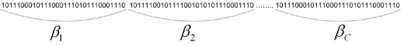
Figure 3: The structure of the PSO particle.

$$\eta_{(f_{c})}=\beta_{f_{c}}*f_{c}$$ (10)

Algorithm 1 WatermarkCreation

0: $EMR$, $f$, Usability Constraints set $\hbar$

0: Betamatrix $\{\beta_{1},\beta{2},.....,\beta_{C}\}$

 Initialize swarm $S_{W}$ of $p$ particles with positions and velocities in the range $(\beta_{min},\beta_{max})$ and $0\leq\upsilon_{i}(0)\leq\upsilon_{max}(0)$ respectively

 for every feature in the $f$ perform the following steps

 for $iter=1$ to $iter_{max}$ do

      for $i=1$ to $p$ do

          note personal best and local best positions

          Use swarm to calculate watermark to insert in $f$ subject to $\hbar$

          Evaluate the fitness of particle $i$ using equation (9)

          if stopping condition has met then

              return $\{\beta_{1},\beta{2},.....,\beta_{C}\}$

          else

              Update personal best and global best positions

          end if

      end for

 end for

 return $\{\beta_{1},\beta{2},.....,\beta_{C}\}$

In the proposed scheme, the watermark value is calculated using the optimized $\beta$ with the help of equation (10). Once the optimum value of $\beta$ for each candidate attribute $f_{c}$ is found, the algorithm is stopped.

For brevity, we have only reported the motion of particles to find the optimum value of $\beta$ – satisfying the constraints ($\hbar$) using the fitness function given in equation (9) – in Figure 4 for a candidate feature with the highest classification potential $C_{P}$. It is evident from the figure that the particles do converge towards an optimum value of a watermark with the progress of PSO. Recall that the motivation of our work is to preserve the classification potential ($C_{P}$) of high ranking features; therefore, we plot $\Delta_{C_{P}}$ – the difference between $C_{P_{W}}$ and $C_{P_{O}}$ – in Figure 4 to substantiate our argument.

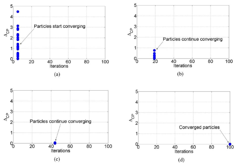
Figure 4: Motion of particles to find optimum value for watermarking subject to $\hbar$.

The benefit of using PSO for calculating $\beta$ prior to watermark insertion is that the process of optimization is not required during the embedding process. As a result, the watermark can be inserted online in realtime into every tuple of EMR. The important steps of watermark creation algorithm are shown in Algorithm 1.

To ensure that the classification potential of a feature is not altered once the watermark is inserted, EMR usability constraints are specified by the set $\hbar$. If a particle violates the usability constraints, its velocity is updated is such a way that it quickly returns to the feasible space. A watermark consisting of $l$ bit strings is generated and the watermark value $\eta$ is added to the value of the feature $f_{c}$ when a given bit is 0; otherwise, its value is subtracted from the features’ value. The algorithm stops when the maximum number of iterations are done or $CP_{O}$ and $CP_{W}$ have approximately equal values for a certain number of iterations.

III-C Watermark Embedding

A bit string of length $l$ is generated as the watermark and the best particle from PSO swarm is used to calculate and embed the watermark value in relevant fields of EMR provided it satisfies the usability constraints set $\hbar$. The watermark value $\eta$ is calculated using the $\beta$ values in equation (10). Since the length of the watermark is $l$; therefore, the watermark value $\eta$ is calculated and inserted $l$ times in the $EMR$. The length l of the watermark should be carefully chosen because: (1) if it is too small, it makes the watermark vulnerable to attacks, and (2) if it is too large, it results in violating the usability constraints. Moreover, the watermark should be created in realtime. After a number of empirical studies, a length of $16$ bits is recommended that meets the above-mentioned requirements. (It is important to emphasize that our algorithm allows a user to chose a watermark length of 8, 16, 32 and 64 bits.)

Algorithm 2 EmbeddingWatermark

0: $EMR$, $WatermarkW={\beta_{1},\beta_{2},...,\beta_{C}}$, $\hbar$

0: $EMR_{W}$, $\Delta$

 for $q=1$ to $C$ do

      for $r=1$ to $R$ do

          if $b_{i}==0$ then

              $EMR_{W(r,q)}\Leftarrow EMR_{(r,q)}+\eta_{(r,q)}$ subject to $\hbar$

          end if

          insert $\eta_{(r,q)}$ into $\Delta$

          if $b_{i}==1$ then

              $EMR_{W(r,q)}\Leftarrow EMR_{(r,q)}-\eta_{(r,q)}$ subject to $\hbar$

          end if

          insert $\eta_{(r,q)}$ into $\Delta$

      end for

 end for

 return $EMR_{W},\Delta$

If the bit is 0 then the value of the selected feature in the matrix $f$ is watermarked by adding $\eta$, which is calculated in the watermark creation step, to its value. If the bit is 1, $\eta$ is subtracted from the value of the selected feature. We use numeric attributes to illustrate the watermark embedding procedure. The watermark is created from Step 2 presented in section III-A. $\Delta$ is a matrix that contains the statistics for each feature $f_{c}$, such as the percentage change $\beta_{f_{c}}$, exact change $\eta$, and the overall change. This matrix is continuously updated during the watermarking embedding process to use it in the decoding stage. The embedding algorithm is run $l$ times to embed the watermark multiple times keeping in view the usability constraints $\hbar$. The Algorithm 2 lists the steps involved in the watermark embedding stage.

III-D Watermark Decoding

In the watermark decoding process, first step is to locate the attributes which have been watermarked. To this end, we again rank the attributes in $EMR_{W}$ using the procedure given in Section III-A1. We propose a novel watermark decoder $\tau$, which calculates the amount of change in the value of a feature that does not effect its classification potential. The watermark decoder decodes the watermark by analyzing one bit at a given time. The decoding phase consists of two steps:

Step 1. For every candidate feature $f_{c}$ of all the rows in $EMR_{W}^{{}^{\prime}}$, the watermark bits are detected starting from LSB (least significant bit) and moving towards MSB (most significant bit). The bits are detected in the reverse order compared with the bits embedding order because it is easy to detect the effect of last embedded bit of the watermark. This process is carried out using the change matrix $\Delta$.

Step 2. The bits are then decoded using a majority voting scheme.

III-E Watermark Decoder

We now define a novel watermark decoder that takes into account the degree of change, depending on its classification potential, tolerated by each feature without violating the usability constraints. It is defined as:

$$\tau_{f_{c}}=\frac{\beta_{f_{c}}}{\gamma},$$ (11)

where $\gamma$ is the correction factor in the range (0, 1) and is always greater than zero.

We have tested the operator with different values of $\beta$ and $\tau_{f_{c}}$ on different $EMRs$ as well. For brevity, we show plot decoding accuracy of our technique on different combinations of $\beta$ and $\tau$ in Figure 5 for only one selected feature from the $EMR_{W}$. The decoding phase of our scheme is dependent on the watermark decoder. The watermark decoder in turn uses the knowledge of percentage change $\beta$ introduced during the watermark embedding stage. As a consequence, our watermark decoder also becomes information-preserving during calculation of $\beta$; and hence decoding errors are reduced.

Our decoding algorithm selects one row at a time, for every watermarked feature, and calculates $\eta_{d_{f_{c}}}$ using the equation:

$$\eta_{d_{f_{c}}}=\beta_{f_{c}}\ast(f_{c_{W}}),$$ (12)

where $\eta_{d(r,_{f_{c}})}$ is the detected amount of change in the value of a feature after an attack on the watermark bit b. The algorithm computes the difference between $\eta_{d_{f_{c}}}$ and $\eta_{{}_{f_{c}}}$ using the equation:

$$\eta_{\Delta_{f_{c}}}=\eta_{d_{f_{c}}}-\eta_{f_{c}}$$ (13)

Where $\eta_{\Delta_{f_{c}}}$ represents the difference between the changes detected in the value of a feature during the decoding process and the changes actually made in its value during the encoding process. This value is compared with the watermark decoder to correctly decode the bit. If $\eta_{\Delta_{f_{c}}}$ for a row $r$ is less than or equal to zero then decoded bit is 1, and if the value of $\eta_{\Delta_{f_{c}}}$ for that row lies between 0 and $\tau$ then the decoded bit is 0. Recall, during the watermark creation process the maximum value of $\beta$ is calculated subject to the usability constraints $\hbar$. Similarly, $\beta$ is used to compute the optimum value of watermark decoder $\tau$; therefore, if for a row $r$ $\eta_{\Delta_{f_{c}}}$ is greater than $\tau$ then the usability constraints must have been violated for that row $r$. In this case, the algorithm decodes the watermark bit as $\times$. For data to remain useful even after attacks, the number of bits decoded as $\times$ will be very small for the whole dataset. As a result, the majority voting used during the watermark decoding process cancels the effects of such bits that ensures high watermark decoding accuracy. After decoding a bit, the next bit is detected using the same process. The watermark decoding steps are depicted in Algorithm 3.

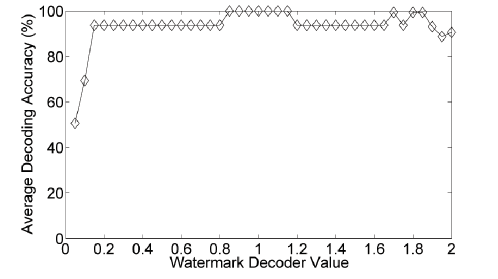
Figure 5: Watermark decoding accuracy for different values of $\tau$.

Algorithm 3 WatermarkDecoding

0: Altered EMR $EMR_{W}^{{}^{\prime}}$, Data Change Matrix $\Delta$, $f_{c}$, $l$

0: Detected Watermark $W_{D}$

 $dt(1,2,...,l)\Leftarrow 0$

 $Ones\Leftarrow 0$

 $Zeros\Leftarrow 0$

 for $q=1$ to $C$ do

      for $b=l$ to $1$ do

          for $r=1$ to $R$ do

              Compute $\eta_{d_{q}}$ and $\eta_{\Delta_{q}}$ using equations (12) and (13) respectively

              if $\eta_{\Delta_{q}}\leq 0$ then

                  $dt(r,b)\Leftarrow 1$

                  $Ones=Ones+1$

              else if $\eta_{\Delta_{q}}>0$ and $\eta_{\Delta_{q}}\leq\tau$ then

                  $dt(r,b)\Leftarrow 0$

                  $Zeros=Zeros+1$

              else {//usability constraints violated}

                  $dt(r,b)\Leftarrow\times$

              end if

          end for

      end for{//Update the data}

      if $Ones>Zeros$ then

          $EMR^{{}^{\prime}}_{W_{q}}=EMR^{{}^{\prime}}_{W_{q}}+\eta_{d(q)}$

      else

          $EMR^{{}^{\prime}}_{W_{q}}=EMR^{{}^{\prime}}_{W_{q}}-\eta_{d(q)}$

      end if

 end for

 $W_{D}\Leftarrow mode(dt(1,2,...,l))$

 return $W_{D}$

The time complexity of our algorithm is $({l*C*R})$ where ${R}$ is the total number of tuples in the database relation, $l$ is the watermark length and $C$ is the number of selected subset features from the relation in the database. Since $l\ll R$ , and $C\ll R$, therefore, for large databases the time complexity of encoding and decoding phases of proposed watermarking technique is $O(R)$. In the following subsection we give an example to highlight the working of our watermark embedding and watermark decoding algorithms.

III-F Example

III-F1 Watermark Encoding

Consider an EMR that has one table with three columns. The third column $D_{1}$ contains the value Yes and No indicating if a patient is suffering from the disease $D_{1}$ or not. Other two columns $A_{1}$ and $A_{2}$ contain numeric values for some vitals of the patient. In order to select the candidate feature for watermarking, we first calculate the classification potential of the features $A_{1}$ and $A_{2}$ using equation (4). After this step, we have identified $A_{1}$ as the candidate feature for watermarking because $A_{2}$, having the highest classification potential should not be watermarked. Suppose after applying the optimization scheme the optimum value of $\beta=1\%$ is found for watermark embedding. Now suppose we want to insert a 5-bits long watermark ”11001” in the EMR. We calculate the value of $\eta$ to embed into $A_{1}$ using the equation:

$$\eta=\beta.A_{1}$$

Our watermark embedding takes the most significant bit (MSB) of the watermark to embed it into $A_{1}$. For this purpose the algorithm works with one row at a time. Now, as the MSB of the watermark is 1, therefore, the new value of $A_{1}$ (we denote it by $A_{1_{W}}$ after embedding this bit will be:

$$A_{1_{W}}=A_{1}-\eta$$

Now, in order to embed second MSB our algorithm again applies the same mechanism, but the updated value of the attribute $A_{1}$ (which was $A_{1_{W}}$ ) is used for calculating new values of $\eta$ and $A_{1_{W}}$ . When our algorithm reaches at third MSB of the watermark then the new value of $A_{1_{W}}$ after embedding this bit would be:

$$A_{1_{W}}=A_{1}+\eta$$

The above mechanism is repeated until all rows of the EMR have been watermarked to generate $EMR_{W}$ . In $EMR_{W}$ both features $A_{1}$ and $A_{2}$ have the same classification potential which they had in EMR. The watermarking process is illustrated in Figure 7.

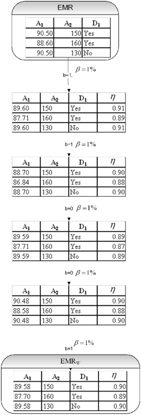
Figure 6: Watermark encoding process with $\beta=1\%$ and watermark $W=11001$.

III-F2 Watermark Decoding

In this phase, the features are again ranked based on their classification potential (calculated using equation (4)). Now the feature with the least classification potential is $A_{1}$. So we have identified the watermarked feature. Now we use the values of $\beta$ (saved during the watermark encoding stage) to calculate the value of $\eta_{D}$ for $A_{1_{W}}$ as follows:

$$\eta_{D}=\beta.A_{1_{W}}$$

We decode the embedded bits in reverse order in which they are encoded, that is, we start from the least significant bit (LSB) and move towards MSB. We use $\eta$ for embedding the last bit of the watermark and compute its difference from the $\eta_{D}$ using the equation:

$$\eta_{\Delta}=\eta_{D}-\eta$$

We compare $\eta_{\Delta}$ with the value of our watermark decoding operator to decode the last embedded watermark bit. After decoding the last embedded bit for all the rows, majority vote is taken and if the output of the majority voting process for that bit is 1 then 1 is saved as the detected bit and the values of feature $A_{1}$ in all the rows is updated using the equation:

$$A_{1_{W}}=A_{1_{W}}+\eta_{D}$$

And if the output of the majority voting is 0 then 0 is saved as the detected bit and the values of feature $A_{1}$ in all the rows is updated using the equation:

$$A_{1_{W}}=A_{1_{W}}-\eta_{D}$$

As mentioned earlier in this paper, the watermark decoding is done in the reverse order of the watermark embedding process: the last embedded bit is decoded first and so on. Therefore, in this example of watermark decoding (depicted in Figure LABEL:fig:WatermarkDecodingExample) the decoded watermark after applying the majority voting scheme on every row of the dataset at every step is 11001, which is same the embedded watermark.

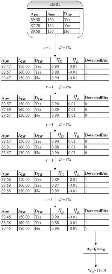
Figure 7: Watermark Decoding process with $\beta=1\%$ and $\tau=1$.

IV Experiments and Results

We have performed extensive experiments to test the effectiveness and accuracy of the proposed watermarking technique. We have applied our technique on two EMRs : (1) an oncology EMR provided for our research by CureMD [http://www.curemd.com] and (2) a Gynaecological EMR used by the authors of [26]. For brevity, we report results on the second EMR that contains more than 200,000 electronic health records. The usability constraints specified in equation (9) are imposed during watermark embedding. We also limit the maximum value of $\beta_{f_{c}}$ to 2%. We have performed our experiments on a Microsoft SQL Server that is running on pentium IV computer with 1.73 GHz core 2 CPU with 1 GB of RAM.

It takes approximately $0.003$ seconds to embed a 16-bit watermark in one feature of a health record. Similarly, it takes less than $0.00026$ seconds per feature per record to decode it. The watermark encoding takes relatively large time because the usability constraints must be satisfied for every bit of the watermark in the encoding process. The watermark decoder $\tau$ is computed using equation (11) to minimize the decoding errors. (In the reported results we use p = 100 particles, g=100, and l=16.)

Recall that we give a choice to the owner of an EMR to chose a watermark length by trading imperceptibility for efficiency. See in Table II to analyze the time required to insert and detect varying length (8, 16, 32 and 64 bits) watermarks. As a rule of thumb, we suggest using 16-bit watermark because it provides very good imperceptibility with acceptable processing overheads.

TABLE II: Watermark creation, insertion and decoding time.

$l$	Creation time	Insertion time	Decoding time
8-bits	14 Milliseconds	1.5 Milliseconds	0.16 Milliseconds
16-bits	27 Milliseconds	3 Milliseconds	0.26 Milliseconds
32-bits	44 Milliseconds	7.6 Milliseconds	0.38 Milliseconds
64-bits	66 Milliseconds	15 Milliseconds	3 Milliseconds

IV-A Watermark Imperceptibility and Data Quality

In this section, we show that once the $EMR$ is watermarked with the proposed scheme, the watermark not only remains imperceptible but also preserves the classification potential of all watermarked features. We use two information theory measures – Kullback - Leibler Divergence ($D_{KL}$) and Jensen-Shannon Divergence ($JSD$) to analyze the similarity between features’ distribution of watermarked and original datasets. The results are tabulated in Table III. For brevity, we report the comparison of pdfs for 2 features from the top and 2 from the bottom of the ranked features, and also plot pdfs for the top ranking feature from both datasets in Figure 8. We show the information-preserving characteristic of our watermarking by classifying the watermarked dataset with the classifiers that are used in Section III-A1. (We also add one more rule-based classifier – C4.5 – to analyze the requirement of preserving diagnosis rules.) We tabulate the classification statistics in Table IV to show effect of watermarking on them.

TABLE III: The comparison between pdfs for $EMR$ and $EMR_{W}$.

Features	Measure
	DKL	JSD
SYSTOLIC_BP	0	0
DIASTOLIC_BP	0	0
TEMPERATURE	0.00001	0.000003
OPEN_OS_SIZE	0.0002	0.00006

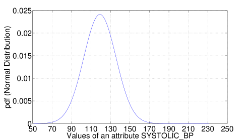
(a) The normal probability density function (pdf) with normal distribution for the attribute $SYSTOLIC\_BP$ in original data.

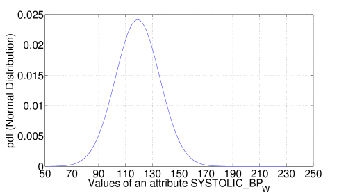
(b) The normal probability density function (pdf) with normal distribution for the attribute $SYSTOLIC\_BP_{W}$ in the watermarked data.

Figure 8: The normal data distribution before and after watermarking an attribute $SYSTOLIC\_BP$ in the EMR. It is clear from the figure that the distribution is preserved when the watermark was embedded.

Remember that the motivation of proposing a information-preserving watermarking scheme is to preserve the diagnosis of a medical dataset. We have also included the scheme of Shehab [14] in our comparative study. It is obvious from Table IV that though the scheme of Shehab is imperceptible but it is not information-preserving because it significantly alters the accuracy of diagnosis. In comparison, our technique has preserved the classification accuracy of different classifiers with the exception of a classifier – C4.5 – where our scheme has improved $FAR$ by reducing the $FP$. We believe this is due to the fact that the proposed scheme considers the correlation present among classification potential of all the candidate attributes for watermarking along with the data usability constraints. In comparison, the technique of Shehab only considers the last three usability constraints given in equation (9) and does not take into account the classification potential of a candidate attribute and its correlation with the decision.

TABLE IV: Effect of different watermarking schemes on various classification statistics.

Classifier	Measure	$EMR$	$EMR_{W_{P}}$	$EMR_{W_{S}}$	$|\Delta_{P}|$	$|\Delta_{S}|$
Bagging	TP	152	152	124	0	18.52
	FP	5	5	5	0	0
	TN	3569	3569	3569	0	0
	FN	30	30	58	0	92.51
	DR(%)	83.52	83.52	68.13	0	18.43
	FAR(%)	0.14	0.14	0.14	0	0
J48	TP	150	151	137	0.75	8.52
	FP	3	3	6	0	100
	TN	3571	3571	3568	0.01	0.1
	FN	32	31	45	2.35	41.22
	DR(%)	82.34	82.96	75.33	0.75	8.51
	FAR(%)	0.08	0.08	0.17	0	112.5
C4.5	TP	150	151	122	0.67	18.67
	FP	3	2	2	33.33	33.33
	TN	3571	3571	3572	0.01	0.03
	FN	32	33	60	3.13	87.5
	DR(%)	82.42	81.87	67.03	0.75	8.51
	FAR(%)	0.08	0.06	0.06	25	25
RBF	TP	61	61	64	0	4.96
	FP	20	19	11	3.77	45.29
	TN	3554	3555	3563	0.02	0.25
	FN	121	121	118	0	2.48
	DR(%)	33.43	33.43	35.08	0	4.94
	FAR(%)	0.56	0.54	0.3	3.57	46.43
NB	TP	125	125	126	0	0.6
	FP	183	187	199	2.26	8.83
	TN	3391	3387	3375	0.11	0.47
	FN	57	57	56	0	1.97
	DR(%)	68.72	68.72	69.13	0	0.6
	FAR(%)	5.12	5.23	5.57	2.15	8.79

IV-B Preserving Classification Potential of High Ranking Features

Our pilot studies reveal, if an $EMR$ is watermarked without the knowledge of classification potential $C_{P}$ of a feature, the diagnosis rules are significantly changed; as a consequence, the misdiagnosis increases. This is a serious issue because if a patient has a disease $A$ and after watermarking of features, the patient is diagnosed for disease $B$. If the treatment of disease $B$ is $100$ times more expensive, then the patient ends up not only receiving expensive but also incorrect treatment. Therefore, a watermarking scheme has to be information-preserving to avoid such scenarios.

In Table V, we show the effect of watermarking on classification potential $C_{P}$. In the table, $C_{P(BW)}$ is the classification potential of a particular feature before watermarking and $C_{P(AW)}$ is the classification potential of that feature after watermarking. It is obvious from Table V that information-preserving watermarking scheme is able to preserve the classification potential of a feature after watermarking; as a result, a patient is still diagnosed accurately. In comparison, the threshold based technique of Shehab alters $C_{P}$ of several features; as a result, the overall classification statistics $C_{S}$ are significantly changed.

TABLE V: Effect of watermarking of $EMR$ on $C_{P}s$ of various features.

Feature Name	$C_{P(BW)}$	$C_{P(AW_{P})}$	$C_{P(AW_{S})}$	$|\Delta_{CP_{P}}|$	$|\Delta_{CP_{S}}|$
SYSTOLIC_BP	17.25	17.25	22.55	0	30.72
DIASTOLIC_BP	15.24	15.24	20.28	0	33.07
USD_OBSTETRICAL_BPD	10.53	10.53	10.91	0	3.61
RANDOM_BLOOD_SUGAR_LEVELS	7.58	7.58	3.92	0	48.28
USD_OBSTETRICAL_FL	7.43	7.43	8.51	0	14.54
GRAVIDA	6.39	6.39	8.52	0	33.33
AGE	5.4	5.4	1.81	0	66.48
PULSE_RATE	4.28	4.28	0.89	0	79.21
HEIGHT	4.1	4.1	0	0	100
PARITYB424MONTHS	3.11	3.11	4.14	0	33.12
RESPIRATORY_RATE	2.94	2.94	3.92	0	33.33
WEIGHT	2.88	2.88	1	0	65.28
PARITYAFTER24MONTHS	2.43	2.43	3.23	0	32.92
RENAL_FUNCTION_UREA	2.09	2.09	1.63	0	22.01
FUNDAL_HEIGHT	2.06	2.06	1.72	0	16.5
PULSE	1.34	1.34	1.64	0	22.39
LFT_ALT	0.83	0.83	1.1	0	32.53
MENARCHE	0.74	0.74	0.99	0	33.78
TLC	0.63	0.63	0.89	0	41.27
RENAL_FUNCTION_CREATININE	0.6	0.6	0.8	0	33.33
STATION	0.6	0.6	0.79	0	31.67
PLATELET_COUNT	0.4	0.4	0	0	100
CF_FUNDAL_HEIGHT	0.38	0.38	0	0	100
APPROX_FETAL_WEIGHT	0.27	0.27	0.36	0	33.33
TEMPERATURE	0.22	0.22	0	0	100
OPEN_OS_SIZE	0.2	0.2	0.26	0	30

Preserving the classification statistics of $EMR$, which in turn preserves the diagnosis rules, is the most important requirement that the proposed technique meets. For brevity, we only show a subset of diagnosis rules for hypertension that are discovered by J48 classifier for the hypertension dataset in Table VI. It is easy to conclude that the diagnosis rules do not change before and after watermarking using our technique. In contrast, the technique of Shehab alters the classification rules. See the additional terms appearing in the diagnosis rules of J48 classifier once it is operating on the dataset that is watermarked with Shehab’s technique. (Remember that the technique of Shehab is not information-preserving because it does not take into account the impact of high ranking features on the diagnosis.) This further validates our idea of ranking features on the basis of classification potential before calculating the watermark.

TABLE VI: Effect of different watermarking techniques on classification rules.

$EMR$	$EMR_{W_{P}}$	$EMR_{W_{S}}$
If SYSTOLIC_BP $<=$ 120 And GRAVIDA $<=$ 1	If SYSTOLIC_BP $<=$ 120 And GRAVIDA $<=$ 1	If SYSTOLIC_BP $<=$ 122 And GRAVIDA $<=$ 1
And APPROX_FETAL_WEIGHT $>$ 1.5 And	And APPROX_FETAL_WEIGHT $>$ 1.5 And	And APPROX_FETAL_WEIGHT $>$ 1.5 And
STATION $>$ 0 And OPEN_OS_SIZE $<=$3.5	And STATION $>$ 0 And OPEN_OS_SIZE $<=$3.5	And STATION $>$ 0 And OPEN_OS_SIZE $<=$3.5
And DIASTOLIC_BP $<=$ 70 Then	And DIASTOLIC_BP $<=$ 70 Then	And HEIGHT $>$ 160.5 Then
Hypertension = Yes	Hypertension = Yes	Hypertension = Yes
If SYSTOLIC_BP $<=$ 120 And GRAVIDA $<=$ 1	If SYSTOLIC_BP $<=$ 120 And GRAVIDA $<=$ 1	If SYSTOLIC_BP $<=$ 122 And GRAVIDA $<=$ 1
And APPROX_FETAL_WEIGHT $>$ 1.5 And	And APPROX_FETAL_WEIGHT $>$ 1.5 And	And APPROX_FETAL_WEIGHT $>$ 1.5 And
STATION $>$ 0 And OPEN_OS_SIZE $<=$3.5	And STATION $>$ 0 And OPEN_OS_SIZE $<=$3.5	And STATION $>$ 0 And OPEN_OS_SIZE $<=$3.5
And DIASTOLIC_BP $>$ 70 Then	And DIASTOLIC_BP $>$ 70 Then	And HEIGHT $<=$ 160.5 Then
Hypertension = No	Hypertension = No	Hypertension = No
If SYSTOLIC_BP $<=$ 120 And GRAVIDA $<=$ 1	If SYSTOLIC_BP $<=$ 120 And GRAVIDA $<=$ 1	If SYSTOLIC_BP $<=$ 122 And GRAVIDA $<=$ 1
And PULSE_RATE $>$ 76 Then	And PULSE_RATE $>$ 76 Then	And PULSE_RATE $<=$ 76 And PULSE_RATE $>$ 74
Hypertension = No	Hypertension = No	And AGE $>$ 26 And AGE $<=$ 32 Then
		Hypertension = No
If SYSTOLIC_BP $<=$ 160 And SYSTOLIC_BP $>$ 120	If SYSTOLIC_BP $<=$ 160 And SYSTOLIC_BP $>$ 120	If SYSTOLIC_BP $<=$ 162 And SYSTOLIC_BP $>$ 122
And HEIGHT $>$ 160.5 And STATION $>$ 2 And	And HEIGHT $>$ 160.5 STATION $>$ 2 And	And HEIGHT $>$ 160.5 And STATION $>$ 2 And
PULSE_RATE $>$ 87 Then	PULSE_RATE $>$ 87 Then	HAEMOGLOBIN_LEVELS $<=$ 8 Then
Hypertension = Yes	Hypertension = Yes	Hypertension = Yes

Moreover, it is equally important to demonstrate that a watermarking technique is also resilient to malicious attacks. During the robustness study, only the proposed technique is evaluated because techniques like Shehab’s do not meet the first requirement because they do not account for the classification potential of any attribute before watermarking it. Moreover they do not give any mechanism to decide which attribute is most suitable for watermarking without disturbing the classification potential of the dataset before and after watermarking. On the other hand, in our technique we first examine the classification potential of each candidate attribute to be watermarked and then the watermark range for each attribute to be watermarked is calculated using equations (5) and (6).

IV-C Resilience to Various Attacks

In this study, different types of attacks are generated on the watermarked data. A watermarking technique must meet two requirements: (1) an intruder is not able to locate the watermark, and (2) an intruder is not able to corrupt the watermark without significantly degrading the quality of data.

Suppose Alice is the owner of an $EMR$ and she embeds a watermark $W$ in the electronic records; as a result, the watermarked EMR is $EMR_{W}$. Alice now wants to share $EMR_{W}$ with Bob. In the meantime, Mallory (an intruder) wants to remove the watermark from the dataset so that Alice is unable to claim ownership of its EMR in a court of law.

The robustness study is conducted with the following assumptions: (1) Mallory does not have access to the original $EMR$, and (2) Mallory does not have the resources to acquire secret information like candidate subset $f_{c}$ data of $EMR$, overall data change $\Delta$, usability constraints $\hbar$, change in a particular feature $\beta_{f_{c}}$, watermark length l, and the watermark decoder $\tau_{f_{c}}$. These assumptions (though realistic) make the task of Mallory relatively difficult because he has to corrupt the watermark without compromising the usability of the medical data. Mallory may calculate the classification potential of features in the watermarked dataset but he has to face a dilemma of preserving the diagnostic rules of the dataset while trying to corrupt the watermark.

Therefore, in a worst case scenario, if he is able to successfully alter the watermarked feature while preserving usability constraints (which he is not aware of), even then our technique is able to successfully extract the watermark because we insert the watermark in each row of the database and an attack on a set of rows does not significantly affect the decoding process to a great extent. Also, to deceive the attacker, apart from low ranking features, we select some high ranking (except top $t$ features with respect to classification potential, where $t$ can be decided by the data owner) features for watermarking with classification potential within a certain threshold such that watermarking them does not alter the classification potential of any feature. And we have used the majority voting scheme that significantly reduces the probability of incorrect decoding on the basis of attacking few rows only. Since the attacker has no knowledge of original data and the embedded watermark, therefore, to corrupt the watermark – he may make random changes in the watermark dataset. So for him, at every trial, the probability of success ($p$) is 0.5 for successfully deleting one watermark bit from one row of the watermarked dataset. But we embed watermark in each row of the dataset and take majority voting while decoding the embedded watermark bit, so attacker has to successfully attack at least half the total number of rows $R$ in the dataset. And attack on one row is independent of the attack on other rows, so according to the multiplication rule of the probability, the probability of successfully attacking $\frac{R}{2}$ rows is $(0.5)^{\frac{R}{2}}$. But practically speaking, EMRs have large number of health records and for such EMRs the probability of successful attack even on a single watermark bit is approximately zero.

successfully attacking a watermark bit is virtually zero.

Therefore, the knowledge of classification potentials of the features will not be useful for him to corrupt the watermark unless he deteriorates the data by violating the usability constraints. This model is validated by the experimental results, that proves resilience of our technique against all types of malicious attacks.

In the robustness study, three attacks are studied: (1) Insertion, (2) Deletion, and (3) Alteration.

IV-D Insertion Attacks

Since we embed watermark in each row, and we do not target the order of tuples during watermark embedding; therefore, insertion of new tuples does not disturb the embedded watermark. In the decoding stage, to achieve high detecting accuracy we take the majority voting over all the rows for detecting the embedded watermark. Moreover, we do not use any marker tuples for watermark embedding hence inserting new rows does not make our scheme vulnerable to synchronization errors (which might occur if insertion of new records perturbs the order of marker tuples.) For insertion attacks, Mallory can utilize two mechanisms to insert new tuples into EMR. He might insert $\alpha$ new records by replicating the original records. In this way, $\alpha$-duplicate records are inserted into EMR. It is clear from Figure 9 that the proposed technique is resilient to $\alpha$-duplicate insertion attack because it does not target any specific tuple(s) for watermark embedding.

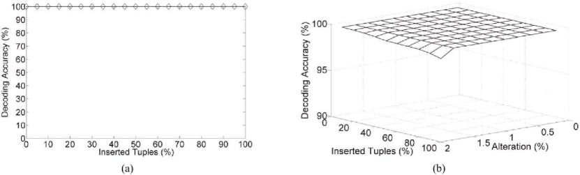
Figure 9: Resilience of proposed technique against various insertion attacks. (a) Resilience to $\alpha$-duplicate insertion attacks. (b) Resilience to $(\alpha,\varrho$) insertion attacks.

The second possibility is to randomly generate fake records and insert them into the EMR. Since Mallory has no information about the original EMR; therefore, he will generate useless records. He may insert new records with the values within the range ($\mu_{W}\pm\varrho\sigma_{W}$) for a specific feature. This type of attack is called ($\alpha,\varrho$)- insertion attacks. It is obvious from Figure 9 that the proposed technique is resilient (generally speaking) to ($\alpha,\varrho$)- insertion attacks and we believe this is because it does not target any specific tuple to insert the watermark.

IV-E Deletion Attacks

In this attack, Mallory deletes selected $\alpha$ tuples from the watermarked dataset $EMR_{W}$. It is the task of the decoding algorithm to recover the watermark from the remaining tuples in each partition. Mallory has to preserve the usability of the dataset, so we assume that deleting tuples does not violate the usability constraints. In particular, if deleting $\alpha$ tuples changes the classification potential of the feature(s) present in the EMR to an extent where overall rank of the features is changed then the diagnosis rules will also change; as a result, the data will not be useful anymore for data mining. Since Mallory is unaware of other usability constraints; therefore, to launch an attack the only option for him is to delete $\alpha$ tuples such that the rank of the features remain intact after the attack. As a consequence, the data remains useful for knowledge driven CDSSs which directly depend on the rank of the features. So, we can realistically assume that Mallory may not be able to alter the ranks of the features while deleting features. Therefore, our technique is able to correctly decode the watermark as long as the features’ ranks are not disturbed. In Figure 10, one can see that even when 80% tuples are deleted, the proposed scheme is able to recover watermark with 100% accuracy. Similarly, when 95% of tuples are deleted, the scheme is still able to recover watermark with an accuracy of 93%. The reason is the same that it does not use marker tuples and also does not insert watermark into specific tuple(s).

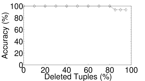
Figure 10: Resilience to deletion attacks.

.

IV-F Alteration Attacks

Mallory can alter the value of an attribute by changing the value of an attribute in a random or fixed manner. In case of random alterations, Mallory selects $\alpha$ tuples and changes the values of features in the range $[0,\pm\varrho]$; hence they are termed as ($\alpha,\varrho$ ) alteration attacks. One can see in Figure 11 that the proposed technique successfully retrieves the watermark even when 60% records are altered. The watermark decoder caters for such data alterations and hence provides robustness against such alterations.

In the second case, Mallory selects $\alpha$ tuples and alters the value of a feature from x to ($x\pm\varrho$). But we see in Figure 11 that the proposed technique is resilient to such fixed alteration attacks as well. This is because the decoding process uses watermark decoder that uses information-preserving watermarking parameter $\beta$.

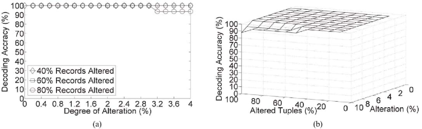
Figure 11: Resilience to alteration attacks. (a) Resilience to random ($\alpha,\varrho$)-alteration attacks. (b) Resilience to fixed ($\alpha,\varrho$)-alteration attacks.

A sophisticated attacker may try to simultaneously launch deletion, insertion, and alteration attacks. In this case, the probability of successful attack is $(o.5)^{\frac{(\alpha+\omega)}{2}}$, where $\alpha$ is the number of records altered, and $\omega$ is the number of unaltered records selected from the watermarked dataset. We have also conducted a number of experiments by changing the percentage of records added, deleted and altered. Our findings are that if an attacker deletes up to 40% (of $R$) of records, adds up to 50%(of $R$) new records, and alters up to 40%(of $R$) records, we are still able to recover the watermark with 100% accuracy.

Moreover, we also study the imperceptibility of the proposed watermarking technique. The objective of this study is to analyze the correlation between the inserted watermark – using our information-preserving watermarking scheme – and the recovered (decoded) watermark using different decoding schemes. The study proves that a watermark inserted with our technique could be successfully decoded using our decoding scheme only. For this purpose, correlation coefficient [31] is used. The results tabulated in Table VII are the average values of correlation coefficient obtained from $100$ different runs of each algorithm. It is clear that the proposed technique achieves the best correlation coefficient through different runs of the algorithms. Any other watermark decoding techniqe never achieves more than $0.16$ correlation coefficient.

TABLE VII: Correlation among watermarks.

l	Proposed Scheme	Shehab’s Scheme	Probabilistic Decoding
8 bits	1	0.16	-0.07
16 bits	1	0.13	-0.22
32 bits	1	0.12	-0.06
64 bits	1	-0.23	0.1

V Conclusion

In this paper, a novel information-preserving technique for watermarking EMR is presented. The benefits of this technique are: (1) preserving the classification potential of high ranking features, (2) empirically selecting the length of watermark to ensure realtime computability constraints, (3) ensuring the usability constraints, and (4) decoding the watermark using majority voting based on a novel watermark decoder. The benefit of using watermark decoder is that it makes the technique resilient to malicious attacks, even in presence of violations of few usability constraints. We have compared the proposed technique with a recently proposed state-of-the-art technique to show that the technique preserves the diagnostic rules of medical data; as a result, the misdiagnosis rate is significantly reduced. To the best of our knowledge, no watermarking technique utilizes the information of classification potential. Moreover, the technique is also resilient to insertion, deletion and alteration attacks. In future, we would like to extend the technique on non-numeric strings data and medical images.

M. Kamran got his BS and MS degree in Computer Science in 2005 and 2008 respectively. Currently he is working as Assistant Professor of Computer Science at COMSATS Institute of Information Technology Wah Campus, Wah Cantt, Pakistan. His research interests include the use of machine learning, evolutionary computations, big data analytic, data security, and decision support systems.

Muddassar Farooq received his B.E. degree in Avionics Engineering from National University of Sciences and Technology (NUST), Pakistan, in 1996. He completed his M.S. in Computer Science and Engineering from University of New South Wales (UNSW), Australia, in 1999. He completed his D.Sc. in Informatics from Technical University of Dortmund, Germany, in 2006. In 2007, he joined the National University of Computer and Emerging Sciences (NUCES), Islamabad, Pakistan, as an associate professor. Currently, he is working as the Director of Next Generation Intelligent Networks Research Center (nexGIN RC). He is the author of the book ”Bee-inspired Protocol Engineering: from Nature to Networks” published by Springer in 2009. He has also coauthored two book chapters in different books on swarm intelligence. He is on the editorial board of Springer s Journal of Swarm Intelligence. He is also the workshop chair of European Workshop on Nature-inspired Techniques for Telecommunication and Networked Systems (EvoCOMNET) held with EuroGP. He also serves on the PC of well known EC conferences like GECCO, CEC, ANTS. He is the guest editor of a special issue of Journal of System Architecture (JSA) on Nature-inspired algorithms and applications. His research interests include agent based routing protocols for fixed and mobile ad hoc networks (MANETs), nature inspired applied systems, natural computing and engineering and nature inspired computer and network security systems, i.e. artificial immune systems.

References

- [1] A. Feldstein, P. Elmer, D. Smith, M. Herson, E. Orwoll, C. Chen, M. Aickin, and M. Swain, “Electronic medical record reminder improves osteoporosis management after a fracture: a randomized, controlled trial,” Journal of the American Geriatrics Society, vol. 54, no. 3, pp. 450–457, 2006.
- [2] http://www.amconmag.com/article/2009/mar/09/00009/, last accessed: January, 20 2011.
- [3] “Electronic health records: A journey to next generation healthcare,” http://www.cognizant.com/html/content/bluepapers/ WP_EHR.pdf, last accessed: January, 20 2011.
- [4] B. Alhaqbani and C. Fidge, “Privacy-Preserving Electronic Health Record Linkage Using Pseudonym Identifiers,” pp. 108–117, 2009.
- [5] M. Peleg, D. Beimel, D. Dori, and Y. Denekamp, “Situation-Based Access Control: Privacy management via modeling of patient data access scenarios,” Journal of Biomedical Informatics, vol. 41, no. 6, pp. 1028–1040, 2008.
- [6] J. Benaloh, M. Chase, E. Horvitz, and K. Lauter, “Patient controlled encryption: ensuring privacy of electronic medical records,” in Proceedings of the 2009 ACM workshop on Cloud computing security. ACM, 2009, pp. 103–114.
- [7] “Emr data theft booming,” http://www.informationweek.com/ news /healthcare/security-privacy/showArticle.jhtml?articleID= 224200494, last updated: 01:24 PM on March 26, 2010, last accessed: January, 20 2011.
- [8] http://www.dailymail.co.uk/news/article-1221186, last updated: 8:13 AM on 18th October 2009, last accessed: January, 20 2011.
- [9] http://www.medicexchange.com/EMR/emr-data-theft-increasing-in-us.html, last accessed: July, 28 2010.
- [10] “Emr data theft booming,” http://www.healthcareitnews.com/ news / patients-sue-walgreens-making-money-their-data, last updated: March 18, 2011, last accessed: July, 12 2011.
- [11] http://www.theregister.co.uk/2005/04/15/ralph_lauren_loses_ data/, last accessed: January, 31 2011.
- [12] R. Agrawal and J. Kiernan, “Watermarking relational databases,” in 28th International Conference on Very Large Data Bases. Morgan Kaufmann Pub, 2002, pp. 155–166.
- [13] R. Sion, M. Atallah, and S. Prabhakar, “Rights protection for relational data,” IEEE Transactions on Knowledge and Data Engineering, pp. 1509–1525, 2004.
- [14] M. Shehab, E. Bertino, and A. Ghafoor, “Watermarking relational databases using optimization-based techniques,” IEEE Transactions on Knowledge and Data Engineering, vol. 20, no. 1, pp. 116–129, 2008.
- [15] R. Agrawal, P. Haas, and J. Kiernan, “Watermarking relational data: framework, algorithms and analysis,” The VLDB journal, vol. 12, no. 2, pp. 157–169, 2003.
- [16] V. Pournaghshband, “A new watermarking approach for relational data,” in Proceedings of the 46th Annual Southeast Regional Conference on XX. ACM, 2008, pp. 127–131.
- [17] R. Hassan, B. Cohanim, O. De Weck, and G. Venter, “A Comparison Of Particle Swarm Optimization And The Genetic Algorithm,” in 46 th AIAA/ASME/ASCE/AHS/ASC Structures, Structural Dynamics, and Materials Conference. American Institute of Aeronautics and Astronautics, 2005, pp. 1–13.
- [18] E. Zitzler, K. Deb, and L. Thiele, “Comparison of multiobjective evolutionary algorithms: Empirical results,” Evolutionary computation, vol. 8, no. 2, pp. 173–195, 2000.
- [19] X. Cui, X. Qin, and G. Sheng, “A weighted algorithm for watermarking relational databases,” Wuhan university journal of natural sciences, vol. 12, no. 1, pp. 79–82, 2007.
- [20] Y. Li, H. Guo, and S. Jajodia, “Tamper detection and localization for categorical data using fragile watermarks,” in Proceedings of the 4th ACM workshop on Digital rights management. ACM, 2004, pp. 73–82.
- [21] Y. Li, V. Swarup, and S. Jajodia, “Fingerprinting relational databases: Schemes and specialties,” IEEE Transactions on Dependable and Secure Computing, vol. 2, no. 1, pp. 34–45, 2005.
- [22] C. Jiang, X. Chen, and Z. Li, “Watermarking Relational Databases for Ownership Protection Based on DWT,” in Proceedings of the 2009 Fifth International Conference on Information Assurance and Security-Volume 01. IEEE Computer Society, 2009, pp. 305–308.
- [23] J. Holland, “Genetic algorithms,” Scientific American, vol. 267, no. 1, pp. 66–72, 1992.
- [24] R. Lewis, V. Torczon, I. for Computer Applications in Science, and Engineering, Pattern search methods for linearly constrained minimization. Citeseer, 1998.
- [25] E. Bertino, B. Ooi, Y. Yang, and R. Deng, “Privacy and ownership preserving of outsourced medical data,” in Data Engineering, 2005. ICDE 2005. Proceedings. 21st International Conference on, 2005, pp. 521–532.
- [26] M. Afridi and M. Farooq, “OG-Miner: an Intelligent Health Tool For Achieving Millennium Development Goals (MDGs) in m-Health Environments,” in Hawaii International Conference on Systems Science, 2011.
- [27] T. Mitchell, “Machine learning. WCB,” Mac Graw Hill, p. 368, 1997.
- [28] J. Kennedy, R. Eberhart et al., “Particle swarm optimization,” in Proceedings of IEEE international conference on neural networks, vol. 4. Piscataway, NJ: IEEE, 1995, pp. 1942–1948.
- [29] G. Renner and A. Ekart, “Genetic algorithms in computer aided design,” Computer-Aided Design, vol. 35, no. 8, pp. 709–726, 2003.
- [30] E. Elbeltagi, T. Hegazy, and D. Grierson, “Comparison among five evolutionary-based optimization algorithms,” Advanced Engineering Informatics, vol. 19, no. 1, pp. 43–53, 2005.
- [31] T. Anderson and T. Anderson, An introduction to multivariate statistical analysis. Wiley New York, 1958.