When does a disaster become a systemic event?
Estimating indirect economic losses from natural disasters

Abstract

Reliable estimates of indirect economic losses arising from natural disasters are currently out of scientific reach. To address this problem, we propose a novel approach that combines a probabilistic physical damage catastrophe model with a new generation of macroeconomic agent-based models (ABMs). The ABM moves beyond the state of the art by exploiting large data sets from detailed national accounts, census data, and business information, etc., to simulate interactions of millions of agents representing each natural person or legal entity in a national economy. The catastrophe model introduces a copula approach to assess flood losses, considering spatial dependencies of the flood hazard. These loss estimates are used in a damage scenario generator that provides input for the ABM, which then estimates indirect economic losses due to the event. For the first time, we are able to link environmental and economic processes in a computer simulation at this level of detail. We show that moderate disasters induce comparably small but positive short- to medium-term, and negative long-term economic impacts. Large-scale events, however, trigger a pronounced negative economic response immediately after the event and in the long term, while exhibiting a temporary short- to medium-term economic boost. We identify winners and losers in different economic sectors, including the fiscal consequences for the government. We quantify the critical disaster size beyond which the resilience of an economy to rebuild reaches its limits. Our results might be relevant for the management of the consequences of systemic events due to climate change and other disasters.

I Introduction

Total economic losses from natural and man-made disasters in 2017 are estimated to be USD 306 billion. With hurricanes Harvey, Irma and Maria, which have made 2017 the second costliest hurricane season on record, the US was hit particularly hard. Due to climate change, economic losses from extreme events – such as floods, droughts, and other climatic disasters – will further increase, and events that have been considered rare until now will become more common in the future (Melillo et al., 2014). However, the resulting economic losses to a national economy are difficult to quantify. While direct losses due to the immediate destruction of homes, firms, infrastructures and lives can be reliably estimated with existing data, estimates of indirect losses – which arise as economic consequences of physical destruction – are much harder to obtain, and no consensus on their validity exists (National Research Council, 1999). The primary reason for this is that natural disasters affect the economy in multiple ways and along several dimensions (Hallegatte and Przyluski, 2010; Linkov et al., 2014). For example, a flood event might destroy or damage the physical capital of a firm, causing output losses and worker layoffs. This, in turn, can trigger further output losses to suppliers and customers of that firm, potentially leading to more layoffs. The associated reduction in household income additionally lowers consumption, potentially further enhancing output losses and increasing layoffs. Subsequently, however, the reconstruction of damaged or destroyed capital can have the opposite effect: companies involved in reconstruction activities experience growth and expand their workforce, which results in higher income that ripples through the economy and leads to economic growth via Keynesian multiplier effects. Hence, natural disasters simultaneously cause both indirect losses and indirect gains. We refer to these losses and gains as indirect economic effects.

Indirect economic effects of average natural disasters, as measured by changes in GDP, are typically small. Net effects may even be close to zero in the short term, where losses and gains of natural disasters can cancel each other out (West, 1996). Still, there are winners and losers, since effects may differ substantially across industries and economic sectors, and almost never cancel for companies and individuals (Loayza et al., 2012). Several empirical studies even find small but positive short- to medium-term overall effects for moderate natural disasters of certain types, especially for moderate floods (Fomby et al., 2013; Loayza et al., 2012; Cavallo et al., 2013; Cunado and Ferreira, 2014; Cavallo et al., 2011; Kousky, 2014; Shabnam, 2014; Leiter et al., 2009). However, the evidence on the sign and magnitude of indirect economic effects of natural disasters in general remains mixed and conflicting, see Cavallo et al. (2011); Kousky (2014); Shabnam (2014) for recent surveys. This situation is echoed in meta-analyses such as Lazzaroni and van Bergeijk (2014), which reports that disasters on average have an insignificant impact in terms of indirect costs, and Klomp and Valckx (2014), which finds some evidence that a part of the negative impact of natural disasters reported in studies is caused by a publication bias. Moreover, (Mohan et al., 2018) shows that the impacts of natural disasters on different components of GDP (such as investment, government and private consumption, exports, imports) differ widely in timing, direction and extent. More aggregate analyses might mask these differences, and it may be difficult to find clear and large net aggregate impacts on GDP. Severe natural disasters (systemic events), on the other hand, are not believed to have neutral or positive economic effects on an aggregate level (Fomby et al., 2013; Cavallo et al., 2013; Loayza et al., 2012; Kousky, 2014; Noy, 2009a; Hochrainer, 2009). Indirect economic losses from these systemic events may be amplified by several mechanisms such as post-disaster inflation, network effects like supply chains affecting firms that were not initially impacted by the event, as well as physical and financial resource constraints regarding the productive capacity of the economy (Hallegatte and Przyluski, 2010). Despite these general arguments, empirical evidence on indirect economic effects of systemic events, particularly regarding severe floods in developed economies, is scarce and largely inconclusive (Fomby et al., 2013; Loayza et al., 2012; Cunado and Ferreira, 2014; Noy and Nualsri, 2007; Jaramillo, 2009a; Cavallo et al., 2013).

Indirect economic effects from natural disasters are difficult to model with traditional approaches such as input-output (IO) models Okuyama and Santos (2014); Hallegatte (2008); Okuyama (2007); Rose and Benavides (1997); Whitman et al. (1997); Boisvert (1992); Cochrane (1997), computable general equilibrium (CGE) models Strulik et al. (2016); Narayan (2003); Rose et al. (2007); Rose and Liao (2005); Brookshire and McKee (1992); Boisvert (1995), and econometric analyses (Fomby et al., 2013; Cavallo et al., 2013; Loayza et al., 2012; Cunado and Ferreira, 2014; Kousky, 2014; Noy, 2009a; Hochrainer, 2009; Cavallo et al., 2011; Leiter et al., 2009; Raddatz, 2009; Kousky, 2014; Shabnam, 2014; Mohan et al., 2018; Lazzaroni and van Bergeijk, 2014; Klomp and Valckx, 2014) because of the over-simplifying nature of these approaches (Rose, 2004). IO models have a tendency to overestimate indirect economic losses and gains (National Research Council, 1999). This was demonstrated, for example, for the case of job gains from reconstruction following the Northridge earthquake in California in 1994: Bolton and Kimbell (1995) showed that the IO estimates by (Cochrane et al., 1996) significantly exceeded actual data for the Los Angeles area following the earthquake (National Research Council, 1999). Furthermore, IO models cannot incorporate the reactions of economic agents to a disaster. By design, CGE models are overly optimistic regarding the flexibility of an economy to react to natural disasters (Hallegatte and Przyluski, 2010). This is due to the underlying assumption that price clearing mechanisms bring the economy back to a general equilibrium after a certain time and are subject only to modest constraints such as adjustment costs in the investment function. However, real-world price formation is sticky and imperfect. Production functions typically assumed in CGE models often overstate the flexibility of substitution between factors of production (labor, capital, material input). Econometric analysis of indirect economic effects faces the problem that statistical, historical relationships used to derive model parameters are likely to be disrupted by the disaster (National Research Council, 1999). The latter study points out an array of factors that may challenge the implicit socio-economic assumptions of the approach, including: the temporary nature of measures taken directly after the disaster event, permanent economic changes (e.g. in the production function), purchase and sale patterns, as well as labor force migration or overtime hours in the reconstruction phase. Indicative of this, West (1996) demonstrates that the regional econometric model results in West and Lenze (1994) over-estimated the economic impact of Hurricane Andrew, which hit the US in 1992, by 70-85 % (National Research Council, 1999).

In summary, traditional approaches so far have failed to provide unambiguous conclusions about the indirect economic effects of natural disasters, in particular regarding systemic events. This means that, given the characteristics of these traditional approaches, today it is still largely impossible to relate the size of initial damages of natural disasters to the expected subsequent indirect economic effects, or to clearly disentangle expected losses and growth effects on a sectoral level. To address this problem, we propose a novel approach that combines a probabilistic physical damage catastrophe model with a new generation of macroeconomic agent-based models (ABMs). The ABM we adopt moves beyond the state of the art by exploiting large data sets from detailed national accounts, census data, and business information, etc., to simulate the interactions of millions of agents representing each natural person or legal entity, such as corporations, government entities and institutions in a national economy. It has been shown that this model is able to forecast numerous macroeconomic variables including major variables such as GDP, inflation, consumption and investment better than standard forecasting approaches (Poledna et al., 2017).

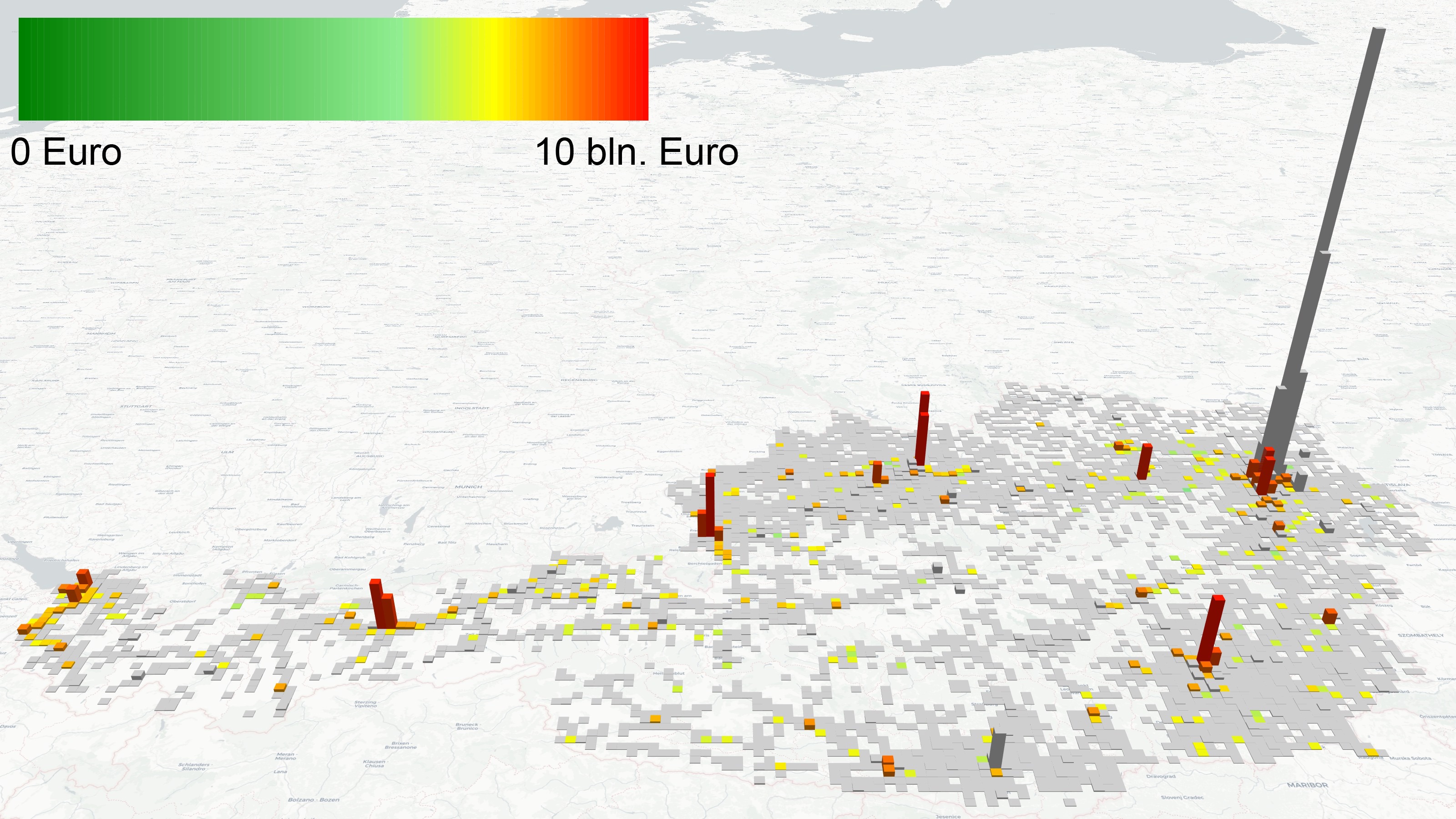
Figure 1: Geospatial distribution of capital across Austria. Affected capital in flooding zones of a 250-year event is shown in a color scale from green to red, where green indicates small damages and red large damages up to 10 bln. Euro. Gray indicates capital stock not affected by the flood. For example, capital stock in Vienna (the large bar in the northeast) is not affected due to extensive flood protection measures, and is therefore shown as grayed out.

We apply our method to estimate indirect economic losses from flood events in Austria, for which the mentioned data is available in highly detailed, complete and consistent form (see SI). The ABM is geolocalized in the sense that the location of capital stock, e.g. firms and infrastructure, is known. The geospatial distribution of capital across Austria is shown in Fig. 1. The physical damage catastrophe model (damage scenario generator) allows us to generate realistic virtual natural disaster events (floods) of controlled size. It is based on a copula approach that assesses realistic hazard frequency and intensity, and takes into account spatial dependencies and the dependency on the severity of the events (see SI). After generating a geolocalized flood event of a given size at the beginning of year 2014, the affected dwellings, firms and infrastructure are destroyed (the affected capital in flooding zones of a 250-year event is depicted in Fig. 1). On this basis, the detailed indirect economic effects across economic sectors and industries are studied in the ABM over several consecutive years.

Results

Moderate disasters do not always have a negative impact on economic growth

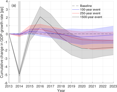
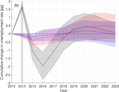
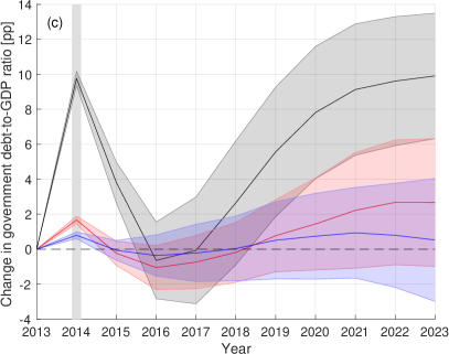
Figure 2: Indirect economic gains and losses of a 100- (blue), 250- (red) and 1,500- (black) year flood event. Time labels on the x-axis indicate the end of each year, and the gray vertical bar marks the first year after the flood. The panels show the effects as percentage point changes relative to the baseline scenario, in which no disaster happens. (a) Cumulative changes in GDP-growth rates. (b) Cumulative changes in the unemployment rate. (c) Changes in the government debt-to-GDP ratio. Shaded areas cover one standard deviation above and below the mean values, as obtained from 50 independent Monte-Carlo simulations.

Fig. 2 shows the indirect economic effects resulting from a 100-year (blue line) and a 250-year (red line) flood event that destroys dwellings and productive capital. The total direct losses (damages) amount to about 0.6 % (100-year event) and 1.2 % (250-year event) of Austrian capital stock, respectively. Fig. 2(a) shows the cumulative change in the GDP growth rate relative to the baseline scenario in percentage points (pp). The qualitative behavior of the two scenarios is similar: starting from small negative effects immediately after the disaster, cumulative effects on economic growth then become positive in the short to medium term (2014-2018), and turn negative in the long term. These effects are most pronounced with an about 0.5 pp cumulative GDP growth rate increase (250-year event) relative to the baseline scenario in the second year after the flood (2015). In the long term, primarily due to a multiplier-accelerator mechanism Samuelson (1939a) (see below), the effects decline to an almost neutral impact (100-year event), and to a reduction of GDP growth of approx. 0.8 pp (250-year event), respectively. This behavior, i.e. positive short- to medium-term and negative long-term effects of moderate size, is in line with the literature (Fomby et al., 2013; Loayza et al., 2012; Cunado and Ferreira, 2014; Leiter et al., 2009; Raddatz, 2009). Fig. 2(b) demonstrates that – as to be expected according to Okun’s law – the change in the unemployment rate is inversely correlated to economic growth, but at a slightly lower amplitude: for the 250-year event, a cumulative decline of almost 0.5 pp two years after the flood (2015) is followed by a cumulative growth in the unemployment rate up to a maximum of about 0.5 pp in the long term. Fig. 2(c) depicts the government debt-to-GDP ratio and shows that the dynamics of the growth and unemployment rates, as well as the transfer we assume to be provided by the government to fully compensate households for their losses of dwellings as catastrophe relief, all lead to an initial rise in this ratio of about 2 pp. For three years after the flood (2015-2018), the government debt-to-GDP ratio temporarily falls slightly below its initial level, but in the long run stabilizes at an increase by more than 2 pp relative to the baseline scenario (250-year event).

Severe disasters have pronouncedly negative economic effects immediately after the event and in the long term

A severe-disaster scenario that simulates a 1500-year flood event is shown in Fig. 2 (black lines). The total direct losses correspond to approximately 10 % of the capital stock in Austria. The indirect economic effects after this shock are qualitatively different from the moderate-disaster scenarios. The initial overall effect on GDP growth is pronouncedly negative, with a cumulative reduction of GDP growth by about 5 pp, see Fig. 2(a). Due to reconstruction, growth picks up fast in the year after the disaster, and surpasses cumulative GDP growth of the baseline scenario by the second year after the flood (2015), culminating in a temporary economic boost of about 2 pp of additional cumulative GDP growth in 2016. The multiplier-accelerator mechanism Samuelson (1939a), as well as production, capacity and credit constraints (see SI) drag growth downwards after this point, leading to negative long-term cumulative growth effects of approx. 1.7 pp. The unemployment rate reacts strongly to the severe disaster, with a cumulative initial increase of more than 1.5 pp, and is followed by a reduction up to almost 2 pp in 2015 during the reconstruction phase, see Fig. 2(b). After this pronounced disruption of the labor market, the unemployment rate rises again by a cumulative change of approx. 0.5 pp (2020) due to the cyclical dynamics, and stabilizes at a level close to the baseline scenario in the long term. Immediately after the disaster, a large initial government transfer to households to compensate for their losses of housing stock, as well as substantial decreases in government revenues and GDP, lead to a 10 pp rise of the government debt-to-GDP ratio, see Fig. 2(c). Even though this ratio shortly returns to its initial level due to the positive economic effects of reconstruction, the downturn because of over-production three years after the flood event implies a subsequent rise in this ratio by almost 10 pp, leaving government finances substantially deteriorated in the long term.

Effects differ substantially across industries and economic sectors

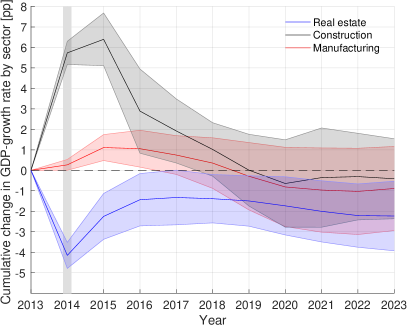
Figure 3: Cumulative growth effects on sectoral GDP after a 250-year flood event for selected economic sectors in percentage points (pp) relative to the baseline scenario. Shaded areas cover one standard deviation above and below the mean values. Sectors shown: construction sector (black), manufacturing sector (red) and real estate sector (blue). The gray vertical bar indicates the year of the flood.

While moderate flood events can have positive aggregate effects in the medium term, impacts are expected to differ significantly across economic sectors. Fig. 3 confirms this conjecture. It shows the effects for the most severely impacted sectors as a result of the 250-year event. The real estate sector (blue line) suffers substantially from the destruction of residential capital stock: sectoral output is reduced by more than 4 pp. Despite reconstruction works improving the initial situation, the cumulative growth change in this sector remains negative, with a cumulative loss in growth of about 2 pp in the long run. The construction sector (black line) immediately profits from the reconstruction of dwellings and productive capital with a sectoral GDP growth of almost 6 pp in the first year after the flood (2014). After the fast ramp-up of reconstruction during the first years after the flood, peaking in an about 6.5 pp increase in the second year after the flood (2015), this effect gradually wears off in the following years, turns slightly negative by year seven after the flood (2020) and remains rather stable at this level thereafter. The restoration of productive capital takes more time. The largest cumulative increase for the manufacturing industry (red line) of about 1 pp is reached in year two after the flood (2015), since this sector supplies a major part of the material input for the re-installment of losses in productive capital. Following the general downturn due to over-production and the thereby induced economic cycle, we see that cumulative GDP growth of this sector in the long term (2019-2023) is lower by almost 1 pp than in the baseline scenario. The effects on all sectors can be found in Table S7 in the SI.

Loss of resilience – when disasters become systemic events

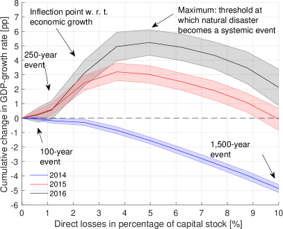
Figure 4: Cumulative changes in GDP growth relative to the baseline scenario as a function of the direct damage as a percentage of GDP. Results are shown for three different years after the disaster: 2014, 2015 and 2016. Shaded areas cover one standard deviation above and below the mean values. Immediately after the event (2014), all disaster sizes are associated with negative growth relative to the baseline scenario. In contrast, for the years 2015 and 2016 there exist inflection points and maxima for GDP growth, indicating the existence of direct damage sizes that, respectively, are “optimal” in terms of economic growth and determine a threshold where natural disasters become systemic events.

Fig. 4 shows the cumulative changes in GDP growth (relative to the baseline scenario) as a function of the sizes of direct damages of the event for different times after the disaster: one year (2014), two years (2015), and three years (2016) after the flood event. As can be expected, the larger the direct damage, the larger the decline of GDP growth immediately after the flooding disaster (2014) is. In the second year after the flood event (2015), the effects of increased economic activity induce positive overall GDP growth. Within this second year, a large part of the initial damage can already by compensated, i.e. cumulative growth effects in the second year are slightly positive, but remain below 1 % for disasters smaller than a 250-year event. For larger events, the economy shows a remarkable growth that is induced by reconstruction after the disaster, which clearly outweighs the direct losses. This growth is limited by different constraining factors (see SI) and starts to decline with respect to the direct losses inflicted by the disaster: the inflection point of the curve occurs at about a 2.4 % loss of capital stock. The cumulative changes in GDP growth in this year show a maximum in the region where the initial damage causes about 3-4 % direct losses in the capital stock. At this maximum, the growth effects lose momentum and indirect losses start to dominate beyond the maximum. The situation is similar for two years after the event (black line): while the position of the inflection point remains at about 2.4 %, the growth stimulus is somewhat more pronounced, and the maximum is located at approximately 5 % direct losses. At this point economic growth is severely restrained, the ability for resilience is lost, and the natural disaster becomes a systemic event.

Discussion

We present a novel approach for estimating the indirect economic losses caused by natural disasters by combining a probabilistic physical damage catastrophe model with a macroeconomic ABM. The method has been applied to flood scenarios in Austria. The ABM is calibrated to the Austrian economy (households, non-financial and financial firms and a government sector) at a scale of 1:1, i.e. every economic agent in Austria (about 10 million) is represented in the model. The ABM incorporates an input-output model with 64 industries, where all goods and services are produced endogenously, and depicts the relevant constraints regarding productive capacities and financing conditions at the level of individual agents. This allows us to estimate the indirect economic effects of natural disasters that are caused by the unfolding sequence of economic events following the initial destruction of productive capital and dwellings. In particular, the model shows the indirect economic effects of simulated disaster shocks of controlled size on the Austrian economy in terms of cumulative GDP growth and other major macroeconomic variables

The model produces realistic results in a number of aspects. Specifically, results correspond well with recent empirical findings of studies including sectoral detail and different types of disasters such as Fomby et al. (2013); Loayza et al. (2012); Cunado and Ferreira (2014); Leiter et al. (2009); Noy (2009a); Raddatz (2009). We find that moderate losses due to 100- and 250-year flood events have small but positive short- to medium-term impacts, while they lead to negative long-term effects of similar magnitude. These results correspond particularly well with Cunado and Ferreira (2014), which shows that floods of moderate magnitude in developed economies, while resulting in positive short- to medium-term effects, have slightly negative cumulative effects in the long run. Short- to medium-term results are further supported by a firm-level empirical study on flooding disasters in Europe (Leiter et al., 2009), which finds higher average firm asset and employment growth for regions affected by flooding disasters. Comparable impacts are also obtained by Loayza et al. (2012); Fomby et al. (2013), which report aggregate short- to medium-term positive growth effects of floods, and by Noy (2009a), which shows that natural disasters have positive short-term growth effects in developed economies. Negative long-term effects for climatic disasters are also reported in Raddatz (2009).

Our study is the first to estimate the indirect economic impacts of severe floods in a developed economy on an empirical basis, at the same time taking account of complex economic interactions and dynamics with our modeling approach. Simulations of severe disasters, such as a 1,500-year flood event in Austria, induce a pronouncedly more negative long-term economic impact on the Austrian economy. These results, in line with a theoretical analysis conducted by Hallegatte et al. (2007), demonstrate that negative indirect effects from severe disasters are primarily due to constraints on the productive capacity of the existing capital stock, credit provision and government finances, which impede immediate reconstruction and thus impose a ceiling on positive growth effects. Empirical findings regarding severe floods are largely inconclusive: Cunado and Ferreira (2014); Fomby et al. (2013); Loayza et al. (2012); Noy and Nualsri (2007); Jaramillo (2009a); Cavallo et al. (2013) all report no, insignificant or (once controlled for) vanishing effects for systemic floods in particular. Especially regarding the most detailed study on flooding disasters (Cunado and Ferreira, 2014), a lack of data on severe floods in developed countries seemed not to have permitted the obtaining of results for this country group.

A unique feature of this analysis is that disaster impacts are disaggregated across 64 industry sectors and simultaneously tracked over time, demonstrating how positive aggregate economic consequences may result in winners and losers subject to particular dynamics. The sectoral decomposition of results reveals that, while some sectors providing the means for the reconstruction of capital stock might profit (predominantly the construction sector, to a lesser extent the manufacturing sector), others that are particularly hit by the disaster suffer from large losses that take several years to be compensated (especially the real estate sector). We compute the distribution of losses and their dynamics over time across sectors at a higher level of detail than previous studies. Models featuring endogenous dynamics such as CGE models, even though they depict up to 35 industry sectors as in Narayan (2003), typically are comparative static CGE models Narayan (2003); Rose et al. (2007); Rose and Liao (2005), while fully dynamic CGE models usually depict only one output good as in Strulik et al. (2016). Furthermore, they often are confined to regions smaller than a national economy (Rose et al., 2007; Rose and Liao, 2005). Sectoral empirical studies such as Fomby et al. (2013); Loayza et al. (2012); Cunado and Ferreira (2014) – besides being limited methodologically as set forth above – typically divide the economy into two to three aggregate sectors (agriculture, industry and/or service sector). IO models applied to comparable contexts, such as Hallegatte (2008), usually exploit the full range of national IO tables (mostly around 60-70 industries), but lack the endogenous non-linear dynamics present in the ABM.

We show that disasters trigger cyclical economic responses that follow a classic multiplier-accelerator mechanism as described in (Samuelson, 1939b). The cycle is caused by an overshooting of investment during the reconstruction phase leading to an economic boom, which is followed by a downturn due to a lack of demand once the restoration of capital stock has been completed. As reported in Fomby et al. (2013); Loayza et al. (2012); Cunado and Ferreira (2014), indirect economic effects immediately after the event are predominantly negative due to initial losses of capital stock, income, as well as demand and supply of goods. The positive economic stimulus due to reconstruction occurs with a delay of at least a quarter, because some time is necessary to compensate for lost capital stock and income. This impulse in turn triggers an economic cycle. In the long term, the consequences of this cycle tend to outweigh the positive economic impact induced by reconstruction activities. Such a cyclical mechanism – which is different from Schumpeter’s creative-destruction or productivity effect, which has been the focus of several studies – has received little attention in the literature up to now, with the exception of a theoretical analysis in Hallegatte and Ghil (2008).

This study is the first to combine a probabilistic physical damage catastrophe model with a macroeconomic ABM to quantitatively relate disaster sizes with the indirect economic impacts. We find a non-trivial behavior of the cumulative GDP growth effects as a function of the direct damage size. We determine a threshold beyond which the full productive capacity of an economy has been exploited to restore destroyed capital stock. At this point, which is at around 5 % of destroyed capital stock, resilience is lost, and economic growth is dominated by direct losses. Previous studies such as Hallegatte et al. (2007) have hitherto investigated this matter on a theoretical and more aggregate basis only.

We believe that in times of increased frequency and severity of potential climate-change-related natural disasters, it is expedient to anticipate their short- to long-term economic implications, direct as well as indirect ones. In particular, it is important to identify potential economic losers of these events, so as to optimally prepare for a fair and efficient post-crisis management.

Materials and methods

Agent based model of a small economy

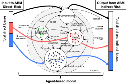
Figure 5: Schematic overview of the ABM structure showing the institutional sectors (households, non-financial and financial firms and a general government), and their interactions. The stacked bars show an example of the distributions of direct (left) and indirect (right) total losses to the government (white), firms (red), and households (blue).

We employ an ABM – developed in Poledna et al. (2017) and Assenza et al. (2015) – which depicts the economy of a small nation at a 1:1 scale (about 10 million agents) (see SI for a model description). The model is based on detailed data sources from national accounts, input-output tables, government statistics, census data and business surveys, and is able to closely approximate time series of major macroeconomic variables (GDP, inflation, household consumption, investment). The basic structure of the model is depicted in Fig. 5. The model is calibrated to the economy of Austria in the year 2013, for which the required data is available (see SI). Large economies are still out of scope for such simulations within reasonable computing time. Simulations were carried out on the supercomputer of the Vienna Scientific Cluster.

Flood risk estimation and damage scenario generator

We estimate the disaster risk distributions for flood losses in Austria using a copula approach, and build a damage-scenario generator based on spatially explicit data to simulate losses to individual households, non-financial and financial firms and government entities across the 64 economic sectors represented in the ABM. The damage-scenario generator simulates a shock to individual agents in the ABM, which subsequently alter their behavior and create higher-order indirect effects over a given time period (see SI).

References

- Melillo et al. (2014) J. M. Melillo, T. Richmond, and G. Yohe, Third National Climate Assessment (2014).
- National Research Council (1999) National Research Council, The impacts of natural disasters: A framework for loss estimation (National Academies Press, 1999).
- Hallegatte and Przyluski (2010) S. Hallegatte and V. Przyluski, The economics of natural disasters: concepts and methods, Tech. Rep. 5507 (The World Bank Policy Research Working Paper, 2010).
- Linkov et al. (2014) I. Linkov, T. Bridges, F. Creutzig, J. Decker, C. Fox-Lent, W. Kröger, J. H. Lambert, A. Levermann, B. Montreuil, J. Nathwani, et al., Nature Climate Change 4, 407 (2014).
- Cochrane (2004) H. C. Cochrane, in Modeling Spatial and Economic Impacts of Disasters (Springer, 2004) pp. 37–52.
- West (1996) C. T. West, in Proceedings of Analyzing Economic Impacts and Recovery from Urban Earthquakes: Issues for Policy Makers, Conference presented by Earthquake Engineering Research Institute and Federal Emergency Management Agency, Pasadena, California (1996).
- Loayza et al. (2012) N. V. Loayza, E. Olaberria, J. Rigolini, and L. Christiaensen, World Development 40, 1317 (2012).
- Fomby et al. (2013) T. Fomby, Y. Ikeda, and N. V. Loayza, Journal of Applied Econometrics 28, 412 (2013).
- Cavallo et al. (2013) E. Cavallo, S. Galiani, I. Noy, and J. Pantano, Review of Economics and Statistics 95(5), 1549 (2013).
- Cunado and Ferreira (2014) J. Cunado and S. Ferreira, Land economics 90, 149 (2014).
- Cavallo et al. (2011) E. Cavallo, I. Noy, et al., International Review of Environmental and Resource Economics 5, 63 (2011).
- Kousky (2014) C. Kousky, Energy Economics 46, 576 (2014).
- Shabnam (2014) N. Shabnam, International Journal of Disaster Risk Science 5, 157 (2014).
- Leiter et al. (2009) A. M. Leiter, H. Oberhofer, and P. A. Raschky, Environmental and Resource Economics 43, 333 (2009).
- Lazzaroni and van Bergeijk (2014) S. Lazzaroni and P. A. van Bergeijk, Ecological Economics 107, 333 (2014).
- Klomp and Valckx (2014) J. Klomp and K. Valckx, Global Environmental Change 26, 183 (2014).
- Mohan et al. (2018) P. S. Mohan, B. Ouattara, and E. Strobl, Ecological Economics 146, 1 (2018).
- Noy (2009a) I. Noy, Journal of Development economics 88, 221 (2009a).
- Hochrainer (2009) S. Hochrainer, World Bank Policy Research Working Paper 4968 (2009).
- Noy and Nualsri (2007) I. Noy and A. Nualsri, University of Harvard Working Paper 07-28 (2007).
- Jaramillo (2009a) C. R. Jaramillo, Documentos CEDE Universidad de Los Andes (2009a).
- Okuyama and Santos (2014) Y. Okuyama and J. R. Santos, Economic Systems Research 26, 1 (2014).
- Hallegatte (2008) S. Hallegatte, Risk analysis 28, 779 (2008).
- Okuyama (2007) Y. Okuyama, Economic Systems Research 19, 115 (2007).
- Rose and Benavides (1997) A. Rose and J. Benavides, Advances in social science analysis of earthquakes, Buffalo, NY: National Center for Earthquake Engineering Research (1997).
- Whitman et al. (1997) R. V. Whitman, T. Anagnos, C. A. Kircher, H. J. Lagorio, R. S. Lawson, and P. Schneider, Earthquake Spectra 13, 643 (1997).
- Boisvert (1992) R. Boisvert, Indirect economic consequences of a catastrophic earthquake , 207 (1992).
- Cochrane (1997) H. Cochrane, Menlo Park, CA: Risk Management Solutions (1997).
- Strulik et al. (2016) H. Strulik, T. Trimborn, et al., Natural disasters and macroeconomic performance, Tech. Rep. (Vienna University of Technology, Institute for Mathematical Methods in Economics, Research Group Economics (ECON), 2016).
- Narayan (2003) P. K. Narayan, Applied Economics Letters 10, 721 (2003).
- Rose et al. (2007) A. Rose, G. Oladosu, and S.-Y. Liao, Risk Analysis 27, 513 (2007).
- Rose and Liao (2005) A. Rose and S.-Y. Liao, Journal of Regional Science 45, 75 (2005).
- Brookshire and McKee (1992) D. Brookshire and M. McKee, Indirect Economic Consequences of a Catastrophic Earthquake , 267 (1992).
- Boisvert (1995) R. Boisvert, Report to the Federal Emergency Management Agency, Ithaca, NY: Cornell University (1995).
- Raddatz (2009) C. Raddatz, The Wrath of God: Macroeconomic Costs of Natural Disasters (World Bank Washington DC, 2009).
- Rose (2004) A. Rose, in Modeling Spatial and Economic Impacts of Disasters. Advances in Spatial Science, edited by C. S. E. Okuyama Y. (Springer, Berlin, Heidelberg, 2004).
- Bolton and Kimbell (1995) N. Bolton and L. Kimbell, in annual meeting of the Population Association of America (1995).
- Cochrane et al. (1996) H. B. Cochrane, B. Kling, D. Black, J. Schmehl, J. Curtsinger, and J. Steenson, in The Economics of Natural Hazards (Univeristy of Colorado, Boulder, 1996).
- West and Lenze (1994) C. T. West and D. G. Lenze, International regional science review 17, 121 (1994).
- Poledna et al. (2017) S. Poledna, M. Miess, and S. Thurner, “Economic forecasting with an agent-based model,” (2017), in preparation.
- Samuelson (1939a) P. A. Samuelson, Review of Economic Statistics 21, 75 (1939a).
- Hallegatte et al. (2007) S. Hallegatte, J.-C. Hourcade, and P. Dumas, Ecological economics 62, 330 (2007).
- Samuelson (1939b) P. A. Samuelson, The Review of Economics and Statistics 21, 75 (1939b).
- Albala-Bertrand (1993) J. M. Albala-Bertrand, The Political Economy of Large Natural Disasters with Special Reference to Developing Countries (Oxford: Clarendon Press, 1993).
- Skidmore and Toya (2002) M. Skidmore and H. Toya, Economic Inquiry Volume 40, Issue 4, 664 (2002).
- Noy (2009b) I. Noy, Journal of Development Economics 88, 221 (2009b).
- Jaramillo (2009b) C. R. H. Jaramillo, Universidad de los Andes, mimeo (2009b).
- Hallegatte and Ghil (2008) S. Hallegatte and M. Ghil, Ecological Economics 68, 582 (2008).
- Assenza et al. (2015) T. Assenza, D. Delli Gatti, and J. Grazzini, Journal of Economic Dynamics and Control 50, 5 (2015).