Markov modeling of peptide folding in the presence of protein crowders

Abstract

We use Markov state models (MSMs) to analyze the dynamics of a $\beta$-hairpin-forming peptide in Monte Carlo (MC) simulations with interacting protein crowders, for two different types of crowder proteins [bovine pancreatic trypsin inhibitor (BPTI) and GB1]. In these systems, at the temperature used, the peptide can be folded or unfolded and bound or unbound to crowder molecules. Four or five major free-energy minima can be identified. To estimate the dominant MC relaxation times of the peptide, we build MSMs using a range of different time resolutions or lag times. We show that stable relaxation-time estimates can be obtained from the MSM eigenfunctions through fits to autocorrelation data. The eigenfunctions remain sufficiently accurate to permit stable relaxation-time estimation down to small lag times, at which point simple estimates based on the corresponding eigenvalues have large systematic uncertainties. The presence of the crowders have a stabilizing effect on the peptide, especially with BPTI crowders, which can be attributed to a reduced unfolding rate $k_{\text{u}}$, while the folding rate $k_{\text{f}}$ is left largely unchanged.

I Introduction

In the crowded interior of living cells, proteins are surrounded by high concentrations of macromolecules, which leads to a reduction of the volume available to a given protein. Under such conditions, steric interactions would universally favor more compact structures. A growing body of evidence indicates, however, that the effects of macromolecular crowding on properties such as protein stability cannot be explained in terms of steric repulsion alone.Guzman et al. (2014); Monteith et al. (2015); Danielsson et al. (2015) To understand the role of other interactions, in recent years, there have been increasing efforts to perform computer simulations with realistic crowder molecules,McGuffee and Elcock (2010); Feig and Sugita (2012); Predeus et al. (2012); Macdonald et al. (2015); Bille et al. (2015); Yu et al. (2016); Feig et al. (2017); Qin and Zhou (2017) rather than hard-sphere crowders. When analyzing these large systems, a major challenge lies in identifying the main states and dynamical modes, which may not be easily anticipated. One possible approach to this problem is provided by Markov modeling techniques,Schütte et al. (1999); Chodera et al. (2007); Buchete and Hummer (2008); Bowman et al. (2009); Prinz et al. (2011) which in recent years have found widespread use in studies of biomolecular processes such as folding and binding.Chodera and Noé (2014); Noé and Clementi (2017) Most of these studies dealt with data from molecular dynamics simulations, but the methods are general and can be used on Monte Carlo (MC) data as well.

In this article, we use Markov modeling, along with time-lagged independent component analysis (TICA),Molgedey and Schuster (1994); Naritomi and Fuchigami (2013); Schwantes and Pande (2013); Pérez-Hernández et al. (2013) to analyze data from MC simulations of a test peptide in the presence of interacting protein crowders, for two different types of crowder proteins. We show that the major free-energy minima and slow dynamical modes of these high-dimensional systems can be identified in a systematic manner using TICA and Markov state models (MSMs). We further show that the dominant MC relaxation times of the peptide can be robustly estimated from the constructed MSMs, although simple estimates based on the MSM eigenvalues are subject to well-known systematic uncertainties. Our procedure for relaxation-time estimation uses the MSM eigenfunctions and autocorrelation fits, rather than the eigenvalues.

As test molecule, we use the $\beta$-hairpin-forming GB1m3 peptide.Fesinmeyer, Hudson, and Andersen (2004) The peptide is simulated in homogeneous crowding environments, where either bovine pancreatic trypsin inhibitor (BPTI) or the B1 domain of streptococcal protein G (GB1) serves as crowding agent. Both these proteins are thermally highly stableMoses and Hinz (1983); Gronenborn et al. (1991) and therefore modeled using a fixed-backbone approximation, whereas the GB1m3 peptide is free to fold and unfold in the simulations. The simulations are conducted using MC dynamics at constant temperature. Recently, we studied the same systems using MC replica-exchange methods, and found that both BPT1 and GB1 have a stabilizing effect on GB1m3.Bille, Mohanty, and Irbäck (2016)

II Methods

II.1 Simulated systems

The simulated systems consist of one GB1m3 molecule and eight crowder molecules, enclosed in a periodic box with side length 95 Å. The eight crowder molecules are copies of a single protein, either BPTI or GB1. This setup yields crowder densities of $\sim$100 mg/mL, whereas the macromolecule densities in cells can be $\sim$300–400 mg/mL.Vendeville, Larivière, and Fourmentin (2011) The volume fraction occupied by the crowders is around 7%. The simulation temperature is set to 332 K, which is near the melting temperature of the free GB1m3 peptide.Fesinmeyer, Hudson, and Andersen (2004) For reference, simulations of the free peptide are also performed, using the same temperature.

The GB1m3 peptide is an optimized variant of the second $\beta$-hairpin (residues 41–56) in protein GB1, with enhanced stability.Fesinmeyer, Hudson, and Andersen (2004) It differs from the original sequence at 7 of 16 positions. To our knowledge, no experimental structure is available for GB1m3, but its native fold is expected to be similar to the parent $\beta$-hairpin in GB1.

II.2 Biophysical model

Our simulations are based on an all-atom protein representation with torsional degrees of freedom, and an implicit solvent force field,Irbäck, Mitternacht, and Mohanty (2009) A detailed description of the interaction potential can be found elsewhere.Irbäck, Mitternacht, and Mohanty (2009) In brief, the potential consists of four main terms, $E=E_{\text{loc}}+E_{\text{ev}}+E_{\text{hb}}+E_{\text{sc}}$. One term ($E_{\text{loc}}$) represents local interactions between atoms separated by only a few covalent bonds. The other, non-local terms represent excluded-volume effects ($E_{\text{ev}}$), hydrogen bonding ($E_{\text{hb}}$), and residue-specific interactions between pairs of side-chains, based on hydrophobicity and charge ($E_{\text{sc}}$). In multi-chain simulations, intermolecular interaction terms have the same form and strength as the corresponding intramolecular ones. The potential is an effective energy function, parameterized through folding thermodynamics studies for a structurally diverse set of peptides and small proteins.Irbäck, Mitternacht, and Mohanty (2009) Previous applications of the model include folding/unfolding studies of several proteins with $>$90 residues.Mitternacht et al. (2009); Jónsson, Mohanty, and Irbäck (2012); Mohanty, Meinke, and Zimmermann (2013); Bille et al. (2013); Jónsson, Mitternacht, and Irbäck (2013); Petrlova et al. (2014) Recently, it was used by us to simulate the peptides trp-cage and GB1m3 in the presence of protein crowders.Bille et al. (2015); Bille, Mohanty, and Irbäck (2016)

Our simulations use the same fully atomistic representation of both the GB1m3 peptide and the crowder proteins. However, because of their high thermal stability,Moses and Hinz (1983); Gronenborn et al. (1991) the crowder proteins are modeled with a fixed backbone, and thus with side-chain rotations as their only internal degrees of freedom. The assumed backbone conformations of BPTI and GB1 are model approximations of the PDB structures 4PTI and 2GB1, derived by MC with minimization. The structures were selected for both low energy and high similarity to the experimental structures. The root-mean-square deviations (RMSDs) from the experimental structures (calculated over backbone and C^β atoms) are $\lesssim$1 Å.

II.3 MC simulations

The systems are simulated using MC dynamics. The simulations are done in the canonical rather than some generalized ensemble. Also, only “small-step” elementary moves are used, so that the system cannot artificially jump between free-energy minima, without having to climb intervening barriers. With these restrictions, the simulations should capture some basics of the long-time dynamics.Tiana, Sutto, and Broglia (2007) Despite the restrictions, the methods are sufficiently fast to permit the study of the folding and binding thermodynamics of the peptide, through simulations containing multiple folding/unfolding and binding/unbinding events.

Our move set consists of four different updates: (i) the semi-local Biased Gaussian Steps (BGS) methodFavrin, Irbäck, and Sjunnesson (2001) for backbone degrees of freedom in the peptide, (ii) simple single-angle Metropolis updates in side chains, (iii) small rigid-body translations of whole chains, and (iv) small rigid-body rotations of whole chains. The “time” unit of the simulations is MC sweeps, where one MC sweep consists of one attempted update per degree of freedom. Specifically, each MC sweep consists of 74 attempted moves in the crowder-free system, whereas the corresponding numbers are 1208 and 1328 with BPTI and GB1 crowders, respectively. Note that the average number of attempted conformational updates of the peptide per MC sweep is the same in all three cases. In the simulations with crowders, the relative fractions of BGS moves, side-chain updates, rigid-body translations and rigid-body rotations are approximately 0.02, 0.94, 0.02 and 0.02, respectively.

All simulations are run with the program PROFASI,Irbäck and Mohanty (2006) using both vector and thread parallelization. To gather statistics, a set of independent runs is generated for each system. The number of runs is 16 with BPTI crowders, 62 with GB1 crowders, and 30 for the isolated peptide. Each run comprises $40\times 10^{6}$ MC sweeps if crowders are present, and $10\times 10^{6}$ MC sweeps without crowders. Compared to the longest relaxation times in the respective systems (see below), the individual runs are a factor $>$20 longer.

Several different properties are recorded during the simulations. As a measure of the nativeness of the peptide, the number of native H bonds present, $n_{\text{hb}}$, is computed, assuming that the native H bonds are the same as in the full GB1 protein (PDB code 2GB1). The interaction of the peptide with surrounding crowder molecules is studied by monitoring intermolecular H bonds and C^α-C^α contacts. A residue pair is said to be in contact if their C^α atoms are within 8 Å.

As input for our TICA and MSM analyses (see below), two sets of parameters are stored at regular intervals during the course of the simulations. The first set consists of all (non-constant) intramolecular C^α-C^α distances within the peptide, called $r_{ij}$. The second set consists of intermolecular distances between the peptide and the crowders, called $d_{ij}$. Specifically, $d_{ij}$ denotes the shortest C^α-C^α distance between peptide residue $i$ and residue $j$ in any of the crowder molecules.

II.4 TICA and MSM analysis

TICA can be used as a dimensionality reduction method. It is somewhat similar to principal component analysis, but identifies high-autocorrelation (or slow) rather than high-variance coordinates. Given time trajectories of a set of parameters, $\{o_{n}\}$ (in our case, the distances $r_{ij}$ and $d_{ij}$, see above), one constructs the time-lagged covariance matrix $c_{nm}(\tau_{\text{cm}})=\langle o_{n}(t)o_{m}(t+\tau_{\text{cm}})\rangle_{t}-\langle o_{n}(t)\rangle_{t}\langle o_{m}(t+\tau_{\text{cm}})\rangle_{t}$, where $\tau_{\text{cm}}$ is the lag time and $\langle\cdot\rangle_{t}$ denotes an average over time $t$. By solving the (generalized) eigenvalue problem $\textbf{C}(\tau_{\text{cm}})\hat{\textbf{v}}_{i}=\hat{\lambda}_{i}\textbf{C}(0)\hat{\textbf{v}}_{i}$, slow linear combinations of the original parameters can be identified. A more advanced method for identifying slow modes is to construct MSMs.

To build an MSM, the state space needs to be discretized. In our calculations, following Ref. (22), the discretization is achieved by clustering the data with the $k$-means algorithmLloyd (1982) in a low-dimensional subspace spanned by slow TICA coordinates. By computing the probabilities of transition among these clusters in a time $\tau_{\text{tm}}$ (which, like $\tau_{\text{cm}}$, is an adjustable parameter), a transition matrix is obtained. Assuming Markovian dynamics, the eigenvectors of this matrix have relaxation times given by

$$\tilde{t}_{i}=-\tau_{\text{tm}}/\ln\tilde{\lambda}_{i}(\tau_{\text{tm}})$$ (1)

where $1=\tilde{\lambda}_{0}>\tilde{\lambda}_{1}\geq\tilde{\lambda}_{2}\geq...>0$ are the eigenvalues. The eigenvalue $\tilde{\lambda}_{0}$ corresponds to a stationary distribution ($\tilde{t}_{0}=\infty$), whereas all other eigenvalues correspond to relaxation modes with finite timescales $\tilde{t}_{i}$. The timescales obtained using Eq. 1 are expected to reproduce the dominant relaxation times of the full system if the discretization is sufficiently fine,Kube and Weber (2007); Djurdjevac, Sarich, and Schütte (2012) or if the lag time is sufficently large.Djurdjevac, Sarich, and Schütte (2012); Prinz, Chodera, and Noé (2014)

There are several software packages available for TICA and MSM analysis.Scherer et al. (2015); Seeber et al. (2010); Biarnés et al. (2012); Harrigan et al. (2017) Our calculations are done using the pyEMMA software.Scherer et al. (2015)

II.5 Timescales from autocorrelations of MSM eigenfunctions

Another way of estimating relaxation times from an MSM is to compute autocorrelations of the eigenfunctions. The (normalized) autocorrelation function of a general property $f$ is given by $C_{f}(\tau)=[\langle f(t)f(t+\tau)\rangle_{t}-\langle f(t)\rangle_{t}\langle f(t+\tau)\rangle_{t}]/\sigma_{f}^{2}$, where $\sigma_{f}^{2}$ is the variance of $f$. Let $\psi_{i}^{\text{MSM}}$ be the $i$th eigenfunction of a given MSM, and let $\psi_{i}$ be the true $i$th eigenfunction of the system’s time transfer operator.Prinz et al. (2011) The autocorrelation function of $\psi_{i}^{\text{MSM}}$, $C_{i}(\tau)$, may be expanded as

$$C_{i}(\tau)=\sum_{j}c_{j}\text{e}^{-\tau/t_{j}}$$ (2)

where $t_{j}$ is the exact $j$th relaxation time. The coefficients $c_{j}$ are given by $c_{j}=|\langle\psi_{j},\psi_{i}^{\text{MSM}}\rangle|^{2}$, where the overlap $\langle\psi_{j},\psi_{i}^{\text{MSM}}\rangle$ can be expressed as an average with respect to the stationary distribution, $\mu(x)$: $\langle\psi_{j},\psi_{i}^{\text{MSM}}\rangle=\int dx\mu(x)\psi_{j}(x)\psi_{i}^{\text{MSM}}(x)$. Note that $\psi_{j}$ and $\psi_{i}^{\text{MSM}}$ have mean zero and unit norm. In Sect. III, overlaps between pairs of general functions are computed in the same way, after shifting and normalizing the functions to zero mean and unit norm.

Now, if $\psi_{i}^{\text{MSM}}$ is a good approximation of $\psi_{i}$, then $c_{j}\ll c_{i}$ for $j\neq i$. If this holds, $C_{i}(\tau)$ decays approximately as $\text{e}^{-\tau/t_{i}}$ for not too large $\tau$ (compared to $t_{i}$), so that $t_{i}$ can be estimated through a simple exponential fit.

The calculations discussed below use data for $C_{i}(\tau)$ in the range of $\tau$ where $0.2<C_{i}(\tau)<0.8$. Over this range, $C_{i}(\tau)$ is to a good approximation single exponential for all MSM eigenfunctions studied. The upper bound on $\tau$ is set primarily by statistical uncertainties, rather than by deviations from single-exponential behavior.

III Results

Our analysis of the GB1m3 peptide in the three simulated systems (with BPTI crowders, with GB1 crowders, without crowders) can be divided into two parts. First, equilibrium free-energy surfaces are constructed, using TICA coordinates. Second, the dynamics are investigated, using MSM techniques.

III.1 Free-energy landscapes

It is instructive to begin with the isolated GB1m3 peptide, whose folding thermodynamics have been studied before using the same model.Irbäck, Mitternacht, and Mohanty (2009) This study found that the isolated peptide folds in a cooperative manner, and that the number of native H bonds present, $n_{\text{hb}}$, is a useful folding coordinate that has a bimodal distribution at the melting temperature. Figure 1a shows the free energy of the isolated GB1m3, calculated as a function of the two slowest TICA coordinates, TIC0 and TIC1. The free-energy surface exhibits two major minima, labeled I and II, which are well separated in the TIC0 direction. From Fig. 1(b), it can be seen this coordinate is strongly (anti-) correlated with $n_{\text{hb}}$. This correlation implies that the peptide is native-like in free-energy minimum I, and unfolded in minimum II.

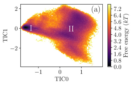
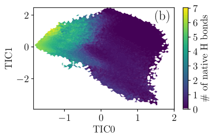
Figure 1: (a) Free energy of the isolated GB1m3 peptide, calculated as a function of the two slowest TICA coordinates, TIC0 and TIC1. Major minima are labeled by Roman numerals. (b) The dependence of the number of native H bonds, $n_{\text{hb}}$, on these coordinates. Here, each stored conformation is represented by a point in the TIC0,TIC1-plane, in a color determined by the value of $n_{\text{hb}}$. Smoothing is applied to improve readability. The TICA lag time is set to $\tau_{\text{cm}}=10^{3}$ MC sweeps.

We now turn to the system where GB1m3 is surrounded by BPTI crowders. Here, the TICA coordinates are linear combinations of both intra- and intermolecular distances ($r_{ij}$ and $d_{ij}$; see Sec. II.3). Calculated as a function of the two slowest TICA coordinates, the free energy exhibits four major minima, labeled I–IV (Fig. 2(a)). To characterize the minima, an interpretation of the TIC0 and TIC1 coordinates is needed. As in the previous case, TIC0 is strongly correlated with $n_{\text{hb}}$ (Fig. 2(b)), and thus linked to the degree of nativeness. Inspection of the eigenvector corresponding to TIC1 suggests that this coordinate depends strongly on certain peptide-crowder distances $d_{ij}$ involving the BPTI residue Pro8, which is part of a sticky patch on the BPTI surface.Bille, Mohanty, and Irbäck (2016) Motivated by this observation, Fig. 2(c) shows the TIC0,TIC1-dependence of a function defined to be unity whenever there is at least one residue-pair contact between the peptide and a Pro8 BPTI residue, and zero otherwise (smoothing is used). This function is indeed strongly correlated with TIC1. Therefore, the main free-energy minima can be classified based on whether or not the peptide is native-like, and whether or not the peptide forms any Pro8 BPTI contact. The peptide is native-like and bound in minimum I, which actually can be split into two distinct subminima, corresponding to two preferred orientations of the folded and bound peptide. In the remaining three main minima, the peptide is either unfolded and bound (minimum II), native-like and unbound (minimum III), or unfolded and unbound (minimum IV).

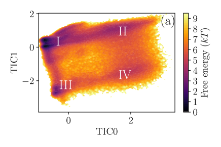
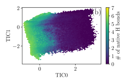
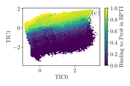
Figure 2: Characterization of the GB1m3 peptide in the presence of BPTI crowders, using the two slowest TICA coordinates, TIC0 and TIC1. (a) Free energy. Major minima are labeled by Roman numerals. (b) The number of native H bonds present in the peptide, $n_{\text{hb}}$. (c) A function which is unity whenever there is at least one residue-pair C^α-C^α contact between the peptide and a Pro8 BPTI residue, and zero otherwise (drawn using smoothing). The contact cutoff distance is 8 Å. The TICA lag time is set to $\tau_{\text{cm}}=10^{3}$ MC sweeps.

With GB1 crowders, the free energy of GB1m3 exhibits five well-separated and easily visible minima (Fig. 3(a)) when calculated as a function of the slowest and third-slowest TICA coordinates.

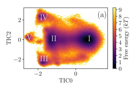
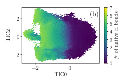
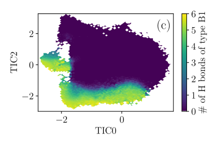
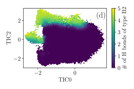
Figure 3: Characterization of the GB1m3 peptide in the presence of GB1 crowders, using the slowest and third-slowest TICA coordinates, TIC0 and TIC2. (a) Free energy. Major minima are labeled by Roman numerals. (b) The number of native H bonds present in the peptide, $n_{\text{hb}}$ (c,d) The numbers of present H bonds associated with the peptide-crowder binding modes B1 and B2 (see the supplementary material, Fig. S2), respectively. The TICA lag time is set to $\tau_{\text{cm}}=20\times 10^{3}$ MC sweeps.

The TIC0,TIC2-plane is used here because two of the minima (III and IV) cannot be distinguished in the TIC0,TIC1-plane (see the supplementary material, Fig. S1). The TIC0 coordinate is again correlated with the degree of nativeness of the peptide (Fig. 3(b)). Proper interpretation of the TIC2 coordinate requires knowledge of the preferred peptide-crowder binding modes. It turns out that there are two preferred binding modes, called B1 and B2. In both cases, binding occurs through $\beta$-sheet extension; the edge strand $\beta$3 (residues 42–46) of GB1 binds to either the first or the second strand of the folded GB1m3 $\beta$-hairpin. The binding modes can be described in terms of the H bonds involved (see the supplementary material, Fig. S2). Figures 3(c) and 3(d) show how the presence of H bonds associated with the respective modes vary with TIC0 and TIC2. Apparently, low and high TIC2 signal B1 and B2 binding, respectively. A similar analysis of TIC1 shows that this coordinate separates bound and unbound states, but discriminates poorly between the B1 and B2 modes (see the supplementary material, Fig. S1(c,d)). The isolated island at low TIC0 and intermediate TIC2 stems from simultaneous binding of the peptide via both modes, to two crowder molecules. Based on the above observations, the free-energy minima in Fig. 3(a) can be described as follows. In minima I and II, the peptide is unfolded and native-like, respectively, and neither B1 nor B2 binding occurs. In the remaining three minima, the peptide is native-like and bound. The mode of binding is either B1 (minimum III), B2 (minimum IV) or both (minimum V).

It is worth noting that the interpretation of the TIC0 coordinates of the BPTI and GB1 systems is not necessarily the same, although TIC0 is a strongly correlated with folding in both cases. In the GB1 system, TIC0 is correlated not only with folding but also with double binding (Fig. 3(c,d)). By contrast, in the BPTI system, the correlation between TIC0 and the binding coordinate is weak (Fig. 2(c)).

To sum up, the results of this section show that TICA provides useful coordinates for describing the free energy of the peptide in the different systems. Using a few slow TICA coordinates, the main free-energy minima can be identified.

III.2 Dynamics

TICA provides a first approximation of the slow modes. For a more detailed investigation of the dynamics of the peptide in our simulations with crowders, MSMs are constructed as described in Sec. II.4, for a range of lag times $\tau_{\text{tm}}$. Relaxation times are estimated by two methods: (i) from MSM eigenvalues (Eq. 1), and (ii) by fits to autocorrelation data for MSM eigenfunctions (Sec. II.5). Illustrations of how the main MSM eigenfunctions are related to the TICA modes discussed above can be found in the supplementary material (Figs. S3–S6).

Figure 4(a) shows estimates of the four longest relaxation times in the system with BPTI crowders, as obtained by the above-mentioned methods. As expected, the eigenvalue-based estimates have systematic errors for small lag times $\tau_{\text{tm}}$. To keep this error low, $\tau_{\text{tm}}$ has to be comparable to the timescale in question. The estimates based on autocorrelation analysis depend, by contrast, only very weakly on $\tau_{\text{tm}}$. This behavior suggests that the true relaxation times can be estimated from the MSM eigenfunctions even if $\tau_{\text{tm}}$ is relatively small. Consistent with this, a further test shows that the shape of the slowest MSM eigenfunction depends only weakly on $\tau_{\text{tm}}$. Here, pairwise overlaps (see Sect. II.5) were computed between variants of this function obtained for different $\tau_{\text{tm}}$. The overlap was $\geq$0.96 for all possible pairs of $\tau_{\text{tm}}$.

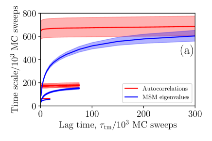
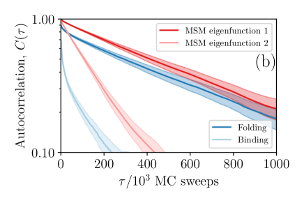
Figure 4: Long-time dynamics of GB1m3 in the presence of BPTI crowders. Shaded areas indicate statistical 1$\sigma$ errors. (a) Estimates of the four longest relaxation times, as obtained using MSM eigenvalues (Eq. 1; blue curves) and autocorrelation analysis (Sec. II.5; red curves). The data are plotted against the lag time $\tau_{\text{tm}}$ of the MSM transition matrix. The second and third longest timescales are very similar. In building the MSMs, data were clustered in the space spanned by the four slowest TICA modes (using $\tau_{\text{cm}}=10^{3}$ MC sweeps), into 800 clusters. (b) Autocorrelation functions, $C(\tau)$, for the two slowest MSM eigenfunctions ($\tau_{\text{tm}}=25\times 10^{3}$ MC sweeps), the folding variable $n_{\text{hb}}$ (Fig. 2(b)), and the binding variable studied in Fig. 2(c).

Figure 4(b) compares the raw autocorrelation functions for the two slowest MSM eigenfunctions to those for the folding and binding coordinates studied in Figs. 2(b) and 2(c), respectively. One observation that can be made is that the autocorrelations of the folding and binding coordinates, not unexpectedly, show clear deviations from single-exponential behavior at small $\tau$. The MSM eigenfunctions are, as intended by construction, much closer to single exponential, which facilitates the extraction of relaxation times.

Another observation from Fig. 4(b) is that, except at small $\tau$, the autocorrelations of the first MSM eigenfunction and the folding coordinate decay at very similar rates. A close relationship between these two functions is indeed suggested from a comparison of Figs. 2(b) and S4(a) (see the supplementary material). This conclusion is further strengthened by their overlap (about 0.88). The autocorrelation function for the second MSM eigenfunction somewhat resembles that for the binding coordinate (Fig. 4(b)), but the overlap is not very large (about 0.36); the binding coordinate overlaps significantly with other MSM eigenfunctions as well. Thus, while the second eigenfunction probably is related to binding, that relationship is not fully captured by the binding coordinate.

Figure 5 shows data from our simulations with GB1 crowders.

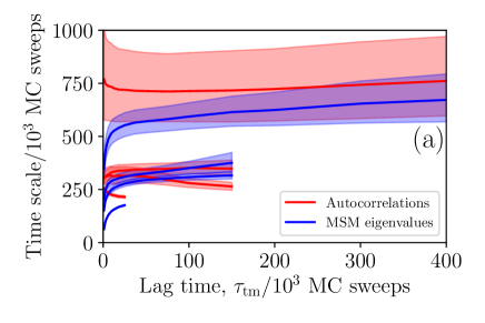
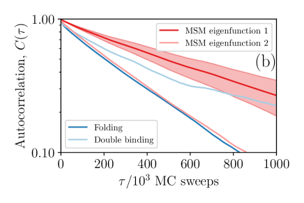
Figure 5: Long-time dynamics of GB1m3 in the presence of GB1 crowders. Shaded areas indicate statistical 1$\sigma$ errors. (a) Estimates of the four longest relaxation times, as obtained using MSM eigenvalues (Eq. 1; blue curves) and autocorrelation analysis (Sec. II.5; red curves). The data are plotted against the lag time $\tau_{\text{tm}}$ of the MSM transition matrix. In building the MSMs, data were clustered in the space spanned by the three slowest TICA modes (using $\tau_{\text{cm}}=20\times 10^{3}$ MC sweeps), into 1574 clusters. (b) Autocorrelation functions, $C(\tau)$, for the two slowest MSM eigenfunctions ($\tau_{\text{tm}}=25\times 10^{3}$ MC sweeps), the folding variable $n_{\text{hb}}$ (Fig. 3(b)), and the binding variable $\chi_{\text{b}}$ (see text). For clarity, statistical errors are shown only for one of the four functions. The statistical uncertainties are somewhat larger for the binding variable $\chi_{\text{b}}$ than they are for the other three functions.

The statistical uncertainties are larger for this system. The main reason for this is that transitions to and from free-energy minimum V (Fig. 3(a)), where the peptide simultaneously binds two crowder molecules, occur only rarely in the simulations. Nevertheless, after increasing the number of runs from 16 for the BPTI system to 62, our total data set contains about 30 independent visits to this minimum, and some clear trends can be seen. The estimated relaxation times follow the same pattern as with BPTI crowders; the estimates based on MSM eigenvalues converge only slowly with increasing $\tau_{\text{tm}}$, whereas those based on autocorrelation analysis are essentially constant down to small $\tau_{\text{tm}}$ (Fig. 5(a)). However, in the GB1 system, the first MSM eigenfunction is more closely linked to binding than to folding. To show this, a binary function sensitive to simultaneous binding of the peptide to two crowder molecules is calculated. Specifically, this function is defined as $\chi_{\text{b}}=\chi_{1}\chi_{2}$, where $\chi_{i}$ is unity if at least three of the H bonds associated with binding mode $i$ (see the supplementary material, Fig. S2) are present, and $\chi_{i}=0$ otherwise. Figure 5(b) shows autocorrelation data for the two slowest MSM eigenfunctions, the folding coordinate ($n_{\text{hb}}$), and the function $\chi_{\text{b}}$. The $n_{\text{hb}}$ and $\chi_{\text{b}}$ functions are natural candidates for the slowest modes, since they are both highly correlated with TIC0. It turns out that the autocorrelation function of $\chi_{\text{b}}$ decays slower than that of $n_{\text{hb}}$, and at a rate comparable to that for the first MSM eigenfunction (Fig. 5(b)). Consistent with this, the first MSM eigenfunction has a larger overlap with the binding function $\chi_{\text{b}}$ (about 0.76) than it has with the folding coordinate (about 0.44).

Finally, we compute and compare the folding and unfolding rates of the peptide, $k_{\text{f}}$ and $k_{\text{u}}$, in the three simulated environments. To this end, we determine the native-state probability, $P_{\text{n}}$ (with the peptide being defined as native if $n_{\text{hb}}\geq 3$), and the apparent folding/unfolding rate, $k=k_{\text{f}}+k_{\text{u}}$. The rate $k$ is obtained by a fit to autocorrelation data for the folding coordinate $n_{\text{hb}}$ (Fig. 6). Knowing $k$ and $P_{\text{n}}$ and assuming a simple folded/unfolded two-state behavior, $k_{\text{f}}$ and $k_{\text{u}}$ can be computed ($k_{\text{f}}=kP_{\text{n}}$, $k_{\text{u}}=k-k_{\text{f}}$).

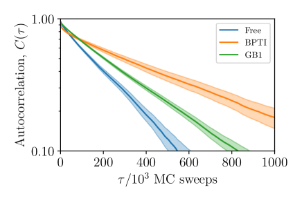
Figure 6: Autocorrelation function, $C(\tau)$, for the folding variable $n_{\text{hb}}$ (the number of native H bonds present in the peptide), as obtained without crowders, with BPTI crowders and with GB1 crowders. Table 1 shows apparent folding rates $k$ obtained by exponential fits to the data. Shaded areas indicate statistical 1$\sigma$ errors.

Our data for $P_{\text{n}}$, $k$, $k_{\text{f}}$ and $k_{\text{u}}$ are summarized in Table 1. The BPTI crowders cause a considerable stabilization of the peptide (increased $P_{\text{n}}$), and a marked decrease in $k$. The decrease in $k$ can be attributed to a lower $k_{\text{u}}$; no significant change in $k_{\text{f}}$ is observed. With GB1 crowders, a similar pattern is observed, although the stabilization of the peptide is much weaker in this case. Again, a markedly reduced $k_{\text{u}}$ is observed, whereas the change in $k_{\text{f}}$ is smaller. Therefore, in both the BPTI and GB1 simulations, the peptide seems to interact more efficiently with the crowders when folded than when unfolded. At the same time, the peptide-crowder interaction is different in character in the BPTI and GB1 cases (see above). Note therefore that the folding of the peptide to its native state entails the formation of both $\beta$-sheet structure and a hydrophobic side-chain cluster, which may enhance the interaction with GB1 and BPTI, respectively.

Table 1: Folding and unfolding rates of the GB1m3 peptide, $k_{\text{f}}$ and $k_{\text{u}}$, in our three simulated systems. The rates are computed from the apparent rate constant $k=k_{\text{f}}+k_{\text{u}}$ and the native-state probability, $P_{\text{n}}$. The peptide is taken as native if at least three native H bonds are present, and $k$ is obtained by fits to the data in Fig. 6. Rates are in units of ($10^{6}$ MC sweeps)^-1.

System	$P_{\text{n}}$	$k$	$k_{\text{f}}$	$k_{\text{u}}$
No crowders	$0.30\pm 0.01$	$3.8\pm 0.3$	$1.1\pm 0.1$	$2.7\pm 0.2$
BPTI crowders	$0.72\pm 0.02$	$1.5\pm 0.2$	$1.1\pm 0.1$	$0.4\pm 0.1$
GB1 crowders	$0.33\pm 0.01$	$2.8\pm 0.1$	$0.9\pm 0.1$	$1.9\pm 0.1$

IV Discussion and summary

In this article, we have analyzed the interplay between peptide folding and peptide-crowder interactions in MC simulations of the GB1m3 peptide with protein crowders, using TICA and MSM techniques. A common major advantage of these methods is that they can be used to search for key coordinates of complex systems in an unsupervised manner. We used the simpler TICA method to explore the free-energy landscape of the peptide. Using a few slow TICA coordinates, it was possible to identify the major free-energy minima of the peptide in the presence of the crowders.

In order to quantitatively analyze the dynamics of the peptide in the simulations, we built MSMs. MSMs offer a convenient method for estimating relaxation times, from the eigenvalues via Eq. 1. However, this method is subject to well-known systematic uncertainties. In particular, it assumes effectively Markovian dynamics, which, at a given level of coarse graining, need not hold for small lag times $\tau_{\text{tm}}$. Unfortunately, in our systems, $\tau_{\text{tm}}$ had to be comparable to the relaxation time in question to keep the systematic error low. Instead, we therefore estimated relaxation times by a procedure based on fits to autocorrelation data for the MSM eigenfunctions. The estimates obtained this way show essentially no $\tau_{\text{tm}}$-dependence. This robustness suggests that the calculated MSM eigenfunctions maintain significant overlaps with the respective true eigenfunctions down to the smallest $\tau_{\text{tm}}$ values used.

It is, of course, also possible to estimate relaxation times from autocorrelation data for other functions than the MSM eigenfunctions. However, the autocorrelation of a general function is a multi-exponential whose parameters may be statistically challenging to determine. The autocorrelation of an MSM eigenfunction should, by contrast, be close to single-exponential over a range of $\tau$, if this eigenfunction approximates the true eigenfunction sufficiently well (at low and high $\tau$, deviations will occur, since the approximation is not perfect). The autocorrelations of our MSM eigenfunctions showed this behavior, and relaxation times could therefore be estimated by single-exponential fits in an intermediate range of $\tau$ (where $0.2<C(\tau)<0.8$). If general functions rather than the MSM eigenfunctions had been used, our possibilities to estimate relaxation times would have been much more limited.

Our simulations further suggest that the GB1m3 peptide interacts more efficiently with both BPTI and GB1 when folded than when unfolded. The addition of either of the crowders led to a reduced unfolding rate $k_{\text{u}}$, while the change in the folding rate $k_{\text{f}}$ was smaller, especially with BPTI crowders.

Supplementary Material

See supplementary material for illustrations of (i) the free energy of GB1m3 with GB1 crowders as a function of the TIC0 and TIC1 coordinates (Fig. S1), (ii) the preferred GB1m3-GB1 binding modes (Fig. S2), and (iii) the character of the leading MSM eigenfunctions in the different systems (Figs. S3–S6).

References

- Guzman et al. (2014) I. Guzman, H. Gelman, J. Tai, and M. Gruebele, J. Mol. Biol. 426, 11 (2014).
- Monteith et al. (2015) W. B. Monteith, R. D. Cohen, A. E. Smith, E. Guzman-Cisneros, and G. J. Pielak, Proc. Natl. Acad. Sci. USA 112, 1739 (2015).
- Danielsson et al. (2015) J. Danielsson, X. Mu, L. Lang, H. Wang, A. Binolfi, F.-X. Theillet, B. Bekei, D. T. Logan, P. Selenko, H. Wennerström, and M. Oliveberg, Proc. Natl. Acad. Sci. USA 112, 12402 (2015).
- McGuffee and Elcock (2010) S. R. McGuffee and A. H. Elcock, PLoS Comput. Biol. 6, e1000694 (2010).
- Feig and Sugita (2012) M. Feig and Y. Sugita, J. Phys. Chem. B 116, 599 (2012).
- Predeus et al. (2012) A. V. Predeus, S. Gul, S. M. Gopal, and M. Feig, J. Phys. Chem. B 116, 8610 (2012).
- Macdonald et al. (2015) B. Macdonald, S. McCarley, S. Noeen, and A. E. van Giessen, J. Phys. Chem. B 119, 2956 (2015).
- Bille et al. (2015) A. Bille, B. Linse, S. Mohanty, and A. Irbäck, J. Chem. Phys. 143, 175102 (2015).
- Yu et al. (2016) I. Yu, T. Mori, T. Ando, R. Harada, J. Jung, Y. Sugita, and M. Feig, eLife 5, 18457 (2016).
- Feig et al. (2017) M. Feig, I. Yu, P.-h. Wang, G. Nawrocki, and Y. Sugita, J. Phys. Chem. B 121, 8009 (2017).
- Qin and Zhou (2017) S. Qin and H.-X. Zhou, Curr. Opin. Struct. Biol. 43, 28 (2017).
- Schütte et al. (1999) C. Schütte, A. Fischer, W. Huisinga, and P. Deuflhard, J. Comput. Phys. 151, 146 (1999).
- Chodera et al. (2007) J. D. Chodera, N. Singhal, V. S. Pande, K. A. Dill, and W. C. Swope, J. Chem. Phys. 126, 155101 (2007).
- Buchete and Hummer (2008) N.-V. Buchete and G. Hummer, J. Phys. Chem. B 112, 6057 (2008).
- Bowman et al. (2009) G. R. Bowman, K. A. Beauchamp, G. Boxer, and V. S. Pande, J. Chem. Phys. 131, 124101 (2009).
- Prinz et al. (2011) J.-H. Prinz, H. Wu, M. Sarich, B. Keller, M. Senne, M. Held, J. D. Chodera, C. Schütte, and F. Noé, J. Chem. Phys. 134, 174105 (2011).
- Chodera and Noé (2014) J. D. Chodera and F. Noé, Curr. Opin. Struct. Biol. 25, 135 (2014).
- Noé and Clementi (2017) F. Noé and C. Clementi, Curr. Opin. Struct. Biol. 43, 141 (2017).
- Molgedey and Schuster (1994) L. Molgedey and H. G. Schuster, Phys. Rev. Lett. 72, 3634 (1994).
- Naritomi and Fuchigami (2013) Y. Naritomi and S. Fuchigami, J. Chem. Phys. 139, 215102 (2013).
- Schwantes and Pande (2013) C. R. Schwantes and V. S. Pande, J. Chem. Theory Comput. 9, 2000 (2013).
- Pérez-Hernández et al. (2013) G. Pérez-Hernández, F. Paul, T. Giorgino, G. De Fabritiis, and F. Noé, J. Chem. Phys. 139, 015102 (2013).
- Fesinmeyer, Hudson, and Andersen (2004) R. M. Fesinmeyer, F. M. Hudson, and N. H. Andersen, J. Am. Chem. Soc. 126, 7238 (2004).
- Moses and Hinz (1983) E. Moses and H.-J. Hinz, J. Mol. Biol. 170, 765 (1983).
- Gronenborn et al. (1991) A. M. Gronenborn, D. R. Filpula, N. Z. Essig, A. Achari, M. Whitlow, P. T. Wingfield, and G. M. Clore, Science 253, 657 (1991).
- Bille, Mohanty, and Irbäck (2016) A. Bille, S. Mohanty, and A. Irbäck, J. Chem. Phys. 144, 175105 (2016).
- Vendeville, Larivière, and Fourmentin (2011) A. Vendeville, D. Larivière, and E. Fourmentin, FEMS Microbiol. Rev. 35, 395 (2011).
- Irbäck, Mitternacht, and Mohanty (2009) A. Irbäck, S. Mitternacht, and S. Mohanty, BMC Biophys. 2, 2 (2009).
- Mitternacht et al. (2009) S. Mitternacht, S. Luccioli, A. Torcini, A. Imparato, and A. Irbäck, Biophys. J. 96, 429 (2009).
- Jónsson, Mohanty, and Irbäck (2012) S. Æ. Jónsson, S. Mohanty, and A. Irbäck, Proteins 80, 2169 (2012).
- Mohanty, Meinke, and Zimmermann (2013) S. Mohanty, J. H. Meinke, and O. Zimmermann, Proteins 81, 1446 (2013).
- Bille et al. (2013) A. Bille, S. Æ. Jónsson, M. Akke, and A. Irbäck, J. Phys. Chem. B 117, 9194 (2013).
- Jónsson, Mitternacht, and Irbäck (2013) S. Æ. Jónsson, S. Mitternacht, and A. Irbäck, Biophys. J. 104, 2725 (2013).
- Petrlova et al. (2014) J. Petrlova, A. Bhattacherjee, W. Boomsma, S. Wallin, J. O. Lagerstedt, and A. Irbäck, Protein Sci. 23, 1559 (2014).
- Tiana, Sutto, and Broglia (2007) G. Tiana, L. Sutto, and R. A. Broglia, Physica A 380, 241 (2007).
- Favrin, Irbäck, and Sjunnesson (2001) G. Favrin, A. Irbäck, and F. Sjunnesson, J. Chem. Phys. 114, 8154 (2001).
- Irbäck and Mohanty (2006) A. Irbäck and S. Mohanty, J. Comput. Chem. 27, 1548 (2006).
- Lloyd (1982) S. Lloyd, IEEE Trans. Inf. Theory 28, 129 (1982).
- Kube and Weber (2007) S. Kube and M. Weber, J. Chem. Phys. 126, 024103 (2007).
- Djurdjevac, Sarich, and Schütte (2012) N. Djurdjevac, M. Sarich, and C. Schütte, Multiscale Model. Simul. 10, 61 (2012).
- Prinz, Chodera, and Noé (2014) J.-H. Prinz, J. D. Chodera, and F. Noé, Phys. Rev. X 4, 011020 (2014).
- Scherer et al. (2015) M. K. Scherer, B. Trendelkamp-Schroer, F. Paul, G. Pérez-Hernández, M. Hoffmann, N. Plattner, C. Wehmeyer, J.-H. Prinz, and F. Noé, J. Chem. Theory Comput. 11, 5525 (2015).
- Seeber et al. (2010) M. Seeber, A. Felline, F. Raimondi, S. Muff, R. Friedman, F. Rao, A. Caflisch, and F. Fanelli, J. Comput. Chem. 32, 1183 (2010).
- Biarnés et al. (2012) X. Biarnés, F. Pietrucci, F. Marinelli, and A. Laio, Comput. Phys. Commun. 183, 203 (2012).
- Harrigan et al. (2017) M. P. Harrigan, M. M. Sultan, C. X. Hernández, B. E. Husic, P. Eastman, C. R. Schwantes, K. A. Beauchamp, R. T. McGibbon, and V. S. Pande, Biophys. J. 112, 10 (2017).