Scattering invariants in Euler’s two-center problem

Abstract.

The problem of two fixed centers was introduced by Euler as early as in 1760. It plays an important role both in celestial mechanics and in the microscopic world. In the present paper we study the spatial problem in the case of arbitrary (both positive and negative) strengths of the centers. Combining techniques from scattering theory and Liouville integrability, we show that this spatial problem has topologically non-trivial scattering dynamics, which we identify as scattering monodromy. The approach that we introduce in this paper applies more generally to scattering systems that are integrable in the Liouville sense.

Keywords: Action-angle coordinates; Hamiltonian systems; Liouville integrability; Scattering map; Scattering monodromy.

1. Introduction

The problem of two fixed centers, also known as the Euler $3$-body problem, is one of the most fundamental integrable problems of classical mechanics. It describes the motion of a point particle in Euclidean space under the influence of the Newtonian force field

$$F=-\nabla V,\ V=-\dfrac{\mu_{1}}{r_{1}}-\dfrac{\mu_{2}}{r_{2}}.$$

Here $r_{i}$ are the distances of the particle to the two fixed centers and $\mu_{i}$ are the strengths (the masses or the charges) of these centers. We note that the Kepler problem corresponds to the special cases when the centers coincide or when one of the strengths is zero.

The (gravitational) Euler problem was first studied by L. Euler in a series of works in the 1760s [19, 20, 21]. He discovered that this problem is integrable by putting the equations of motion in a separated form. Elliptic coordinates, which separate the problem and which are now commonly used, appeared in his later paper [21] and, at about the same time, in the work of Lagrange [36]. The systematic use of elliptic coordinates in classical mechanics was initiated by Jacobi, who used a more general form of these coordinates to integrate, among other systems, the geodesic flow on a triaxial ellipsoid; see [29] for more details.

Since the early works of Euler and Lagrange the Euler problem and its generalizations have been studied by many authors. First classically and then, since the works of Pauli [45] and Niessen [43] in the early 1920s, also in the setting of quantum mechanics. We indicatively mention the works [5, 52, 18, 10, 50, 51, 14, 47]. For a historical overview we refer to [44, 26].

In the present work we will be interested in the spatial Euler problem. For us, it will be important that this problem is a Hamiltonian system with two additional structures: it is a scattering system and it is also integrable in the Liouville sense. The structure of a scattering system comes from the fact that the potential

$$V(q)\to 0,\ \|q\|\to\infty,$$

decays at infinity sufficiently fast (is of long range). It allows one to compare a given set of initial conditions at $t=-\infty$ with the outcomes at $t=+\infty$. An introduction to the general theory of scattering systems can be found in [11, 33]. Liouville integrability comes from the fact that the system is separable; the three commuting integrals of motion are:

• the energy function — the Hamiltonian,

• the separation constant; see Subsection 2.1,

• the component of the angular momentum about the axis connecting the two centers.

An introduction to the general theory of Liouville integrable systems can be found in in [3, 8, 33].

Separately these two structures of the Euler problem have been discussed in the literature. Scattering has been studied, for instance, in [31, 47]. The corresponding Liouville fibration has been studied in [51] — from the perspective of Fomenko theory [25, 3], action coordinates and Hamiltonian monodromy [12]. We will consider both of the structures together and show that the Euler problem has non-trivial scattering invariants, which we will call purely scattering and mixed scattering monodromy, cf. [32, 2, 13, 39, 16]. For completeness, the qualitatively different case of Hamiltonian monodromy will be also discussed. We note that the approach that we introduce in the present paper applies more generally to systems that are both scattering and integrable in the Liouville sense.

The paper is organized as follows. The problem is introduced in Section 2. Bifurcation diagrams are given in Section 3. In Section 4 we discuss classical potential scattering theory. In Section 5 we adapt the discussion of Section 4 to the context of scattering systems that are integrable in the Liouville sense. In particular, we give a definition of a reference system for integrable systems. We note that the choice of a reference system is important for the definition of scattering monodromy; see Subsection 5.2. For the Euler problem, scattering monodromy is discussed in detail in Section 6. Hamiltonian monodromy is addressed in Subsection 6.3. The main part of the paper is concluded with a discussion in Section 7. Additional details are presented in the Appendix.

2. Preliminaries

We start with the $3$-dimensional Euclidean space $\mathbb{R}^{3}$ and two distinct points in this space, denoted by $o_{1}$ and $o_{2}.$ Let $q=(x,y,z)$ be Cartesian coordinates in $\mathbb{R}^{3}$ and let $p=(p_{x},p_{y},p_{z})$ be the conjugate momenta in $T^{*}_{q}\mathbb{R}^{3}$. The Euler two-center problem can be defined as a Hamiltonian system on $T^{*}(\mathbb{R}^{3}\setminus\{o_{1},o_{2}\})$ with a Hamiltonian function $H$ given by

(1) $$H=\frac{\|p\|^{2}}{2}+V(q),\ \ V(q)=-\dfrac{\mu_{1}}{r_{1}}-\dfrac{\mu_{2}}{r_{2}},$$

where $r_{i}\colon\mathbb{R}^{3}\to\mathbb{R}$ is the distance to the center $o_{i}$. The strengths of the centers $\mu_{i}$ can be both positive and negative; without loss of generality we assume that the center $o_{1}$ is stronger, that is, $|\mu_{2}|\leq|\mu_{1}|$.

Remark 2.1.

When $\mu_{i}>0$ (resp., $\mu_{i}<0$) the center $o_{i}$ is attractive (resp., repulsive). The cases $\mu_{1}\neq\mu_{2}=0$ and $\mu_{2}\neq\mu_{1}=0$ correspond to a Kepler problem. In the case $\mu_{1}=\mu_{2}=0$ the dynamics is trivial and we have the free motion $(t,q_{0},p_{0})\mapsto(q_{0}+tp_{0},p_{0})$.

2.1. Separation and integrability

Without loss of generality we assume $o_{i}=(0,0,(-1)^{i}a)$ for some $a>0$, so that, in particular, the fixed centers $o_{1}$ and $o_{2}$ are located on the $z$-axis in the configuration space. Rotations around the $z$-axis leave the potential function $V$ invariant. It follows that (the $z$-component of) the angular momentum

(2) $$L_{z}=xp_{y}-yp_{x}$$

commutes with $H$, that is, $L_{z}$ is a first integral. It is known [52, 18] that there exists another first integral given by

(3) $$G=H+\frac{1}{2}(L^{2}-a^{2}(p_{x}^{2}+p_{y}^{2}))+a(z+a)\frac{\mu_{1}}{r_{1}}-a(z-a)\frac{\mu_{2}}{r_{2}},$$

where $L^{2}=L_{x}^{2}+L_{y}^{2}+L_{z}^{2}$ is the squared angular momentum. The expression for the integral $G$ can be obtained using separation in elliptic coordinates, as described below. It will follow from the separation procedure that the function $G$ commutes both with $H$ and with $L_{z}$, which means that the problem of two fixed centers is Liouville integrable.

Consider prolate ellipsoidal coordinates $(\xi,\eta,\varphi)$:

(4) $$\xi=\frac{1}{2a}(r_{1}+r_{2}),\ \ \eta=\frac{1}{2a}(r_{1}-r_{2}),\ \ \varphi=\textup{Arg}(x+iy).$$

Here $\xi\in[1,\infty),\,\eta\in[-1,1]$, and $\varphi\in\mathbb{R}/2\pi\mathbb{Z}.$ Let $p_{\xi},p_{\eta},p_{\varphi}=L_{z}$ be the conjugate momenta and $l$ be the value of $L_{z}$. In the new coordinates the Hamiltonian $H$ has the form

(5) $$H=\dfrac{H_{\xi}+H_{\eta}}{\xi^{2}-\eta^{2}},$$

where

$$H_{\xi}=\frac{1}{2a^{2}}(\xi^{2}-1)p_{\xi}^{2}+\frac{1}{2a^{2}}\frac{l^{2}}{\xi^{2}-1}-\frac{\mu_{1}+\mu_{2}}{a}\xi$$

and

$$H_{\eta}=\frac{1}{2a^{2}}(1-\eta^{2})p_{\eta}^{2}+\frac{1}{2a^{2}}\frac{l^{2}}{1-\eta^{2}}+\frac{\mu_{1}-\mu_{2}}{a}\eta.$$

Multiplying Eq. (5) by $\xi^{2}-\eta^{2}$ and separating we get the first integral

$$G=\xi^{2}H-H_{\xi}=\eta^{2}H+H_{\eta}.$$

In original coordinates $G$ has the form given in Eq. (3). Since $L_{z}=p_{\varphi}$, the function $G$ commutes both with $H$ and with $L_{z}$.

2.2. Regularization

We note that in the case when one of the strengths is attractive, collision orbits are present and, consequently, the flow of $H$ on $T^{*}(\mathbb{R}^{3}\setminus\{o_{1},o_{2}\})$ is not complete. This complication is, however, not essential for our analysis since collision orbits, as in the Kepler case, can be regularized. More specifically, there exists a $6$-dimensional symplectic manifold $(P,\omega)$ and a smooth Hamiltonian function $\tilde{H}$ on $P$ such that

1. $(T^{*}(\mathbb{R}^{3}\setminus\{o_{1},o_{2}\},dq\wedge dp)$ is symplectically embedded in $(P,\omega)$,

2. $H=\tilde{H}|_{T^{*}(\mathbb{R}^{3}\setminus\{o_{1},o_{2}\})}$,

3. The flow of $\tilde{H}$ on $P$ is complete.

This result is essentially due to [31, Proposition 2.3], where a similar statement is proved for the gravitational planar problem. The planar problem in the case of arbitrary strengths can be treated similarly (note that collisions with a repulsive center are not possible). The spatial case follows from the planar case since collisions occur only when $L_{z}=0$. We note that the integrals $L_{z}$ and $G$ can be also extended to $P$.

One important property of the regularization is that the extensions of the integrals to $P$, which will be also denoted by $H$, $L_{z}$ and $G$, form a completely integrable system. In particular, the Arnol’d-Liouville theorem [1] applies. In what follows we shall work on the regularized space $P$.

3. Bifurcation diagrams

Before we move further and discuss scattering in the Euler problem, we shall compute the bifurcation diagrams of the integral map $F=(H,L_{z},G)$, that is, the set of the critical values of this map. We distinguish two cases, depending on whether $L_{z}$ is zero or different from zero. The bifurcation diagrams are obtained by superimposing the critical values found in these two cases. By a choice of units we assume that $a=1$.

3.1. The case $L_{z}=0$

Since $L_{z}=0$, the motion is planar. We assume that it takes place in the $xz$-plane. Consider the elliptic coordinates $(\lambda,\nu)\in\mathbb{R}\times S^{1}[-\pi,\pi]$ defined by

$$x=\sinh\lambda\cos\nu,\ z=\cosh\lambda\sin\nu.$$

The level set of constant $H=h,L_{z}=l=0$ and $G=g$ in these coordinates is given by the equations

$$p^{2}_{\lambda} =2h\cosh^{2}\lambda+2(\mu_{1}+\mu_{2})\cosh\lambda-2g,$$

$$p^{2}_{\nu} =-2h\sin^{2}\nu-2(\mu_{1}-\mu_{2})\sin\nu+2g,$$

where $p_{\lambda}$ and $p_{\nu}$ are the momenta conjugate to $\lambda$ and $\nu.$ The value $(h,0,g)$ is critical when the Jacobian matrix corresponding to these equations does not have a full rank. Computation yields lines

$$\ell_{1}=\{g=h+\mu_{2}-\mu_{1},l=0\},\ \ell_{2}=\{g=h+\mu_{1}-\mu_{2},l=0\}\\ \mbox{ and }\ \ell_{3}=\{g=h+\mu,l=0\},\ \mu=\mu_{1}+\mu_{2},$$

and two curves

$$\{g =\mu\cosh\lambda/2,\ h=-\mu/2\cosh\lambda,\ l=0\},$$

$$\{g =(\mu_{1}-\mu_{2})\sin\nu/2,\ h=(\mu_{2}-\mu_{1})/2\sin\nu,\ l=0\}.$$

Points that do not correspond to any physical motion must be removed from the obtained set (allowed motion corresponds to the regions where the squared momenta are positive).

Remark 3.1.

The corresponding diagrams in the planar problem are given in Appendix B; see Fig. 5 and 6. We note that in the planar case the set of the regular values of $F$ consists of contractible components and hence the topology of the regular part of the Liouville fibration is trivial. Interestingly, this is not the case if the dimension of the configuration space is $n=3$.

We note that the singular Liouville foliation has non-trivial topology already in the planar case. The corresponding bifurcations, in the sense of Fomenko theory [23, 24, 25, 4, 3], have been studied in [51, 30].

3.2. The case $L_{z}\neq 0$

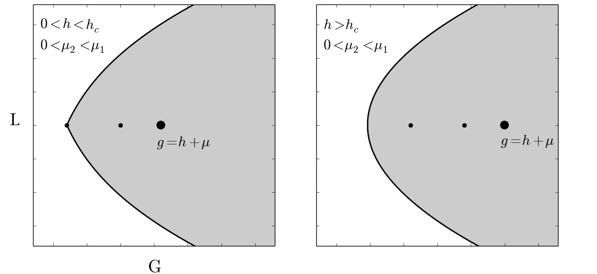
Figure 1. Positive energy slices of the bifurcation diagram for the spatial Euler problem, attractive case. The black points correspond to the critical lines $\ell_{i}$.

In order to compute the critical values in this case it is convenient to use the ellipsoidal coordinates $(\xi,\eta)$. (We note that for $L_{z}\neq 0$ the $z$-axis is inaccessible, so $(\xi,\eta)$ are non-singular.) The level set of constant $H=h,L_{z}=l$ and $G=g$ in these coordinates is given by the equations

$$p^{2}_{\xi} =\dfrac{(\xi^{2}-1)(2h\xi^{2}+2(\mu_{1}+\mu_{2})\xi-2g)-l^{2}}{(\xi^{2}-1)^{2}},$$

$$p^{2}_{\eta} =\dfrac{(1-\eta^{2})(-2h\eta^{2}-2(\mu_{1}-\mu_{2})\eta+2g)-l^{2}}{(1-\eta^{2})^{2}}.$$

The value $(h,l,g)$ with $l\neq 0$ is critical when the corresponding Jacobian matrix does not have a full rank. Computation yields the following sets of critical values:

$$\left\{g=h(2\xi^{2}-1)+\dfrac{(\mu_{1}+\mu_{2})(3\xi^{2}-1)}{2\xi},l^{2}=-\dfrac{(\mu_{1}+\mu_{2}+2h\xi)(-1+\xi^{2})^{2}}{\xi}\right\},$$

$$\left\{g=h(2\eta^{2}-1)+\dfrac{(\mu_{1}-\mu_{2})(3\eta^{2}-1)}{2\eta},l^{2}=-\dfrac{(\mu_{1}-\mu_{2}+2h\eta)(-1+\eta^{2})^{2}}{\eta}\right\},$$

where $\xi>1$ and $-1<\eta<1$. As above, points that do not correspond to any physical motion must be removed.

Representative positive energy slices in the gravitational case $0<\mu_{2}<\mu_{1}$ are given in Fig. 1. The case of arbitrary strengths $\mu_{i}$ is similar. The structure of the corresponding diagrams can partially be deduced from the diagrams obtained in the planar case; see Appendix B.

4. Classical scattering theory

In this section we discuss certain qualitative aspects of scattering theory following [32, 33]. In Section 5 we explain how the theory can be adapted to the context of scattering systems that are integrable in the Liouville sense, with the Euler problem as the leading example.

4.1. Preliminary remarks

Classical scattering theory goes back to the works of Cook [6], Hunziker [28] and Simon [48]. Since then it has received considerable interest and has been actively developed in several directions; see [27, 32, 11, 2, 13].

In the framework of classical scattering one considers two Hamiltonian functions $H$ and $H_{r}$ such that their flows become similar ‘at infinity’. This allows one can compare a given distribution of particles, that is, initial conditions, at $t=-\infty$ with their final distribution at $t=+\infty$. To be more specific, consider a pair of Hamiltonians on $T^{*}\mathbb{R}^{n}$ given by

$$H=\frac{1}{2}\|p\|^{2}+V(q)\mbox{ \ and \ }H_{r}=\frac{1}{2}\|p\|^{2}+V_{r}(q),$$

where the (singular) potentials $V$ and $V_{r}$ are assumed to satisfy a certain decay assumption; see Subsection 4.2. For scattering Hamiltonians the comparison will be achieved in two steps. First we shall parametrize the possible initial and final distributions using the flow of the ‘free’ Hamiltonian $H_{0}=\frac{1}{2}\|p\|^{2}$. Then, for a given invariant manifold, we shall construct the scattering map, where only $H$ and $H_{r}$ are compared.

Remark 4.1.

One reason for such a procedure is the following. As we shall see later in Section 5 and Appendix C, the ‘free’ Hamiltonian is not a natural reference Hamiltonian for the Euler problem, unless the strengths $\mu_{1}=\mu_{2}$. However, the ‘free’ Hamiltonian will be convenient for the definition of the asymptotic states.

Remark 4.2.

In what follows we sometimes refer to $H,H_{r}$ as scattering Hamiltonians and to $H_{r}$ is a reference Hamiltonian for $H$. We note that the ‘reference’ dynamics of $H_{r}$ is usually chosen to be simpler than the ‘original’ dynamics of $H$.

4.2. Decay assumptions

In classical potential scattering the potential function $V\colon\mathbb{R}^{n}\to\mathbb{R}$ of a Hamiltonian $H=\frac{1}{2}\|p\|^{2}+V(q)$ is assumed to decay according to one of the following estimates:

• Finite-range: $\textup{supp}(V)\subset\mathbb{R}^{n}$ is compact;

• Short-range case: $|\partial_{k}V(q)|<c{(\|q\|+1)}^{-|k|-\varepsilon};$

• Long-range case: $|\partial_{k}V(q)\|<c{(\|q\|+1)}^{-|k|-1-\varepsilon}.$

Here $c$ and $\varepsilon$ are positive constants, $k=(k_{1},\ldots,k_{n})\in\mathbb{N}_{0}^{n}$ is a multi-index, $|k|=k_{1}+\ldots+k_{n}$ is a norm of $k$ and $\|q\|$ denotes the Euclidean norm of $q$. For instance, any Kepler potential is of long range and the same is true of the potential found in the Euler problem.

We will assume the potentials $V$ and $V_{r}$ are short-range relative to some decaying rotationally symmetric potentials $\widetilde{V}$ and $\widetilde{V}_{r}$, respectively. For the potential $V$ this means that

$$\|\partial_{k}V-\partial_{k}\widetilde{V}\|<c{\|q\|}^{-|k|-1-\varepsilon},$$

where $\widetilde{V}$ is rotationally symmetric with $\widetilde{V}(q)\to 0,\|q\|\to\infty.$ A similar estimate is assumed to hold for $V_{r}-\widetilde{V}_{r}.$

Remark 4.3.

The potentials $\widetilde{V}$ and $\widetilde{V}_{r}$ are needed to guarantee that the asymptotic direction and the impact parameter are defined and parametrize the scattering trajectories in a continuous way. This is known to be the case for short-range potentials $V$ [33]. Our case reduces to the case of symmetric potentials and in that case the statement follows from the conservation of the angular momentum.

4.3. Asymptotic states

The Hamiltonian flow $g_{H}^{t}\colon P\to P$ of $H$ partitions the (regularized) phase space $P$ into the following invariant subsets:

$$b^{\pm}=\{x\in P\mid\textup{sup}_{t\in\mathbb{R}^{\pm}}\|g_{H}^{t}(x)\|<\infty\}\ \mbox{ and }\ s^{\pm}=\{x\in P\mid H(x)>0\}\setminus b^{\pm}.$$

The invariant subsets

$$b=b^{+}\cap b^{-},\ s=s^{+}\cap s^{-}\ \mbox{ and }\ trp=(b^{+}\setminus b^{-})\cup(b^{-}\setminus b^{+})$$

are the sets of the bound, the scattering and the trapped states, respectively. We note that $s^{-},s^{+}$ and hence $s=s^{-}\cap s^{+}$ are open subsets of $P$.

If the potential $V$ is short-range relative to a decaying rotationally symmetric potential, then the following limits

$${\hat{p}}^{\pm}(x)=\lim_{t\to\pm\infty}p(t,x)\ \mbox{ and }\ q_{\bot}^{\pm}(x)=\lim_{t\to\pm\infty}\left(q(t,x)-\langle q(t,x),{\hat{p}}^{\pm}(x)\rangle\frac{{\hat{p}}^{\pm}(x)}{2h}\right),$$

where $h=H(x)>0$ is the energy of $g_{H}^{t}(x)$, are defined for any $x\in s^{\pm}$ and depend continuously on $x$. These limits are called the asymptotic direction and the impact parameter of the trajectory $g_{H}^{t}(x)$, respectively. We note that an asymptotic direction is always orthogonal to the corresponding impact parameter. Due to the $g_{H}^{t}$-invariance of ${\hat{p}}^{\pm}$ and $q_{\bot}^{\pm}$, we have the maps

$$A^{\pm}=(\hat{p}^{\pm},q_{\bot}^{\pm})\colon s/g^{t}_{H}\to AS$$

from $s/g^{t}_{H}$ to the asymptotic states $AS\subset\mathbb{R}^{n}\times\mathbb{R}^{n}$. Here $s/g^{t}_{H}$ is the space of trajectories in $s$, that is, it is a quotient space of $s$ by the equivalence relation where two points are considered equivalent if and only if they belong to a single trajectory $g^{t}_{H}(x)$. Similarly, one can construct the maps

$$A_{r}^{\pm}=(\hat{p}^{\pm},q_{\bot}^{\pm})\colon s_{r}/g^{t}_{H_{r}}\to AS$$

for the ‘reference’ Hamiltonian $H_{r}=\frac{1}{2}p^{2}+V_{r}(q).$

4.4. Scattering map

Using the maps $A^{\pm}$ and $A^{\pm}_{r}$ constructed in Subsection 4.3, we can now define the notion of a scattering map for a given invariant submanifold $R$ of $s$.

Definition 4.4.

Let $R$ be a $g_{H}^{t}$-invariant submanifold of $s$ and $B=R/g_{H}^{t}$. Assume that the composition map

$$S=(A^{-})^{-1}\circ A^{-}_{r}\circ(A^{+}_{r})^{-1}\circ A^{+}$$

is well defined and maps $B$ to itself. The map $S$ is called the scattering map (w.r.t. $H,H_{r}$ and $B$).

Remark 4.5.

Due to the decay assumptions the maps

$$A^{\pm}\colon s/g_{H}^{t}\to AS\ \mbox{ and }\ A_{r}^{\pm}\colon s_{r}/g_{H}^{t}\to AS$$

are homeomorphisms onto their images in $AS$. It follows that the scattering map $S\colon B\to B$ is a homeomorphism as well. Here the sets $s/g_{H}^{t}$, $s/g_{H}^{t}$ and $B$ are endowed with the quotient topology.

4.5. Knauf’s topological degree

To get qualitative information about the scattering it is useful to look at topological invariants of the scattering map. An important example in the context of general scattering theory is Knauf’s topological index; see [32, 34]. We shall now recall its definition.

Consider the case when the potential $V$ is short-range relative to $V_{r}=0$. Let $h>0$ be a non-trapping energy, that is, a positive energy such that the energy level $H^{-1}(h)$ contains no trapping states, and let $R=H^{-1}(h)\cap s$ be the intersection of the level $H^{-1}(h)$ with the set $s$ of the scattering states. There is the following result.

Theorem 4.6.

([11, 32]) The scattering manifold $B=R/g^{t}_{H}$ is the cotangent bundle $T^{*}S^{n-1}$, where $S^{n-1}$ is the sphere of asymptotic directions. The corresponding scattering map

$$S_{h}\colon B\to B$$

is a symplectic transformation of $T^{*}S^{n-1}$.

Knauf’s topological degree is defined as a topological invariant of $S_{h}$. Specifically, let $\Pr\colon T^{*}S^{n-1}\to S^{n-1}$ be the canonical projection and

$$S^{n-1}_{p}=T^{*}_{p}S^{n-1}\cup\{\infty\}$$

be the one-point compactification of the cotangent space $T^{*}_{p}S^{n-1}$.

Definition 4.7.

(Knauf, [32]) The degree $\textup{deg}(h)$ of the energy $h$ scattering map $S_{h}$ is defined as the topological degree of the map

$$\Pr\circ S_{h}\colon S^{n-1}_{p}\to S^{n-1}.$$

Remark 4.8.

We note that by continuity $\textup{deg}(h)$ is independent of the choice of the initial direction $p\in S^{n-1}$; see [32].

The following theorem shows that for regular (that is, everywhere smooth) potentials $\textup{deg}(h)$ is either $0$ or $1$, depending on the value of the energy $h$; see Fig. 2. We note that for singular potentials, such as the Kepler potential, values different from $0$ and $1$ may appear.

Theorem 4.9.

(Knauf-Krapf, [34]) Let $V$ be a regular short-range potential and $h>0$ be a non-trapping energy. Then

$$\textup{deg}(h)=\begin{cases}0,\ \ h\in(\sup V,\infty),\\ 1,\ \ h\in(0,\sup V).\par\end{cases}$$

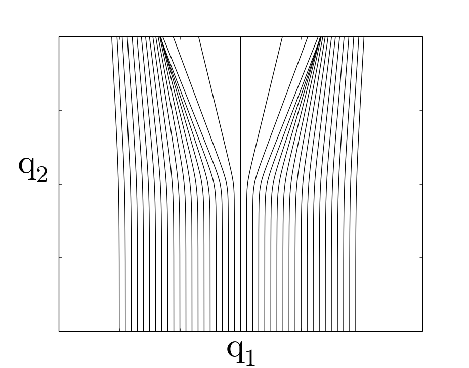
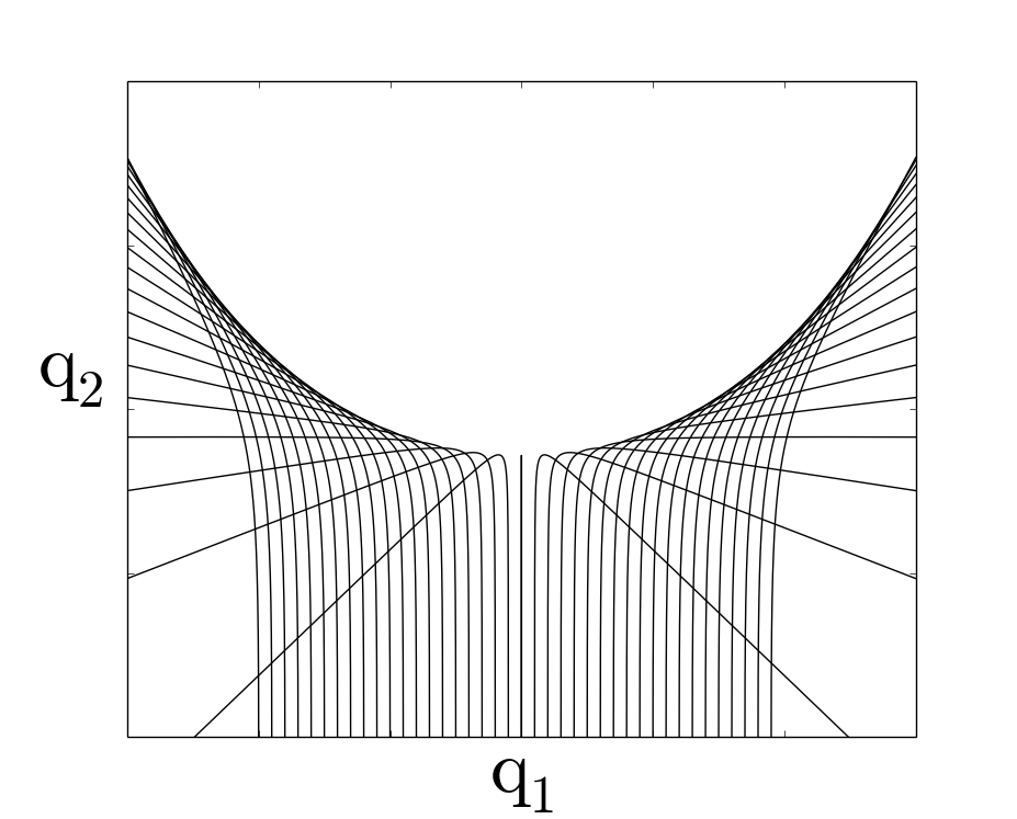
Figure 2. Scattering at different energies. At high energies $\textup{deg}(h)=0$ (left), at low energies $\textup{deg}(h)=1$ (right).

Remark 4.10.

For the Euler problem with $\mu_{1}\mu_{2}\neq 0$, Knauf’s degree is not defined (every positive energy $h$ is trapping). Moreover, the free flow is not a proper reference unless $\mu_{1}=\mu_{2}$; see Section 5. Nonetheless, as we shall show in Sections 5 and 6, for a proper choice of a reference Hamiltonian and a scattering manifold, an analogue of Knauf’s degree can be defined.

5. Scattering in integrable systems

The goal of the present section is to recast the above theory of scattering in the context of Liouville integrability. The approach developed in the present section will be applied to the Euler problem in Section 6.

5.1. Reference systems

As we have seen in Section 4, reference systems can be used to define a scattering map, which is a map between the asymptotic states at $t=-\infty$ and $t=+\infty$ of a given invariant manifold. For integrable systems, natural invariant manifolds are the fibers of the corresponding integral map $F$ and various unions of these fibers. It is thus natural to require that the flow of a reference Hamiltonian maps the set of asymptotic states of a given fiber of $F$ to the set of asymptotic states of the same fiber. This leads to the following definition.

Definition 5.1.

Consider a scattering Hamiltonian $H$ which gives rise to an integrable system $F\colon P\to\mathbb{R}^{n}$. A scattering Hamiltonian $H_{r}$ will be called a reference Hamiltonian for this system if

$$F\left(\lim\limits_{t\to+\infty}g^{t}_{H_{r}}(x)\right)=F\left(\lim\limits_{t\to-\infty}g^{t}_{H_{r}}(x)\right)$$

for every scattering trajectory $t\mapsto g^{t}_{H_{r}}(x)$.

Remark 5.2.

We note that Definition 5.1 can be generalized to the case of scattering and integrable systems defined on abstract symplectic manifolds. However, for the purpose of the present paper it is sufficient to assume that $H$ and $H_{r}$ are as in Section 4.

Remark 5.3.

In scattering theory it is usually required that the flow of a reference Hamiltonian maps the set of asymptotic states of a given energy level to itself, which is a less restrictive assumption. Our point of view is that for integrable systems conserved quantities, such as the angular momentum, should also be taken into account.

A series of examples of reference Hamiltonians in the above sense is given by rotationally symmetric potentials. This follows from the conservation of angular momentum. Another example is the Euler problem. We recall that the Hamiltonian of this problem is given by

$$H=\frac{\|p\|^{2}}{2}-\dfrac{\mu_{1}}{r_{1}}-\dfrac{\mu_{2}}{r_{2}}.$$

Let $F=(H,L_{z},G)\colon P\to\mathbb{R}^{3}$ be the integral map defined in Section 2. We have the following result.

Theorem 5.4.

Among all Kepler Hamiltonians only

$$H_{r_{1}}=\frac{1}{2}p^{2}-\dfrac{\mu_{1}-\mu_{2}}{r_{1}}\ \mbox{ and }\ H_{r_{2}}=\frac{1}{2}p^{2}-\dfrac{\mu_{2}-\mu_{1}}{r_{2}}$$

are reference Hamiltonians of the Euler problem $F=(H,L_{z},G)$. In particular, the free Hamiltonian is a reference Hamiltonian of the Euler problem only in the case $\mu_{1}=\mu_{2}$.

Proof.

See Appendix C. ∎

Remark 5.5.

It follows from Theorem 5.4 that a Kepler Hamiltonian with the strength $\mu_{1}+\mu_{2}$ is not a reference of $F=(H,L_{z},G)$, no matter where the center of attraction, resp., repulsion, is located. For the strength $\mu_{1}+\mu_{2}$ and only for this strength, the difference between the potentials is short-range. This implies that the Møller transformations (or the wave transformations) [33, 11] are not defined with respect to the reference Hamiltonians $H_{r_{i}}$, unless the reference flow is appropriately modified. We note that the existence of Møller transformations is important for the study of quantum scattering in this problem.

5.2. Scattering invariants

Consider the Liouville fibration $F\colon s\to\mathbb{R}^{n}$. Let $H_{r}$ be a reference Hamiltonian for $F$ such that $A^{\pm}(s)\subset A^{\pm}(s_{r})$ holds. Setting $R=s$, we get the scattering map

$$S\colon B\to B,\ B=R/g^{t}_{H}.$$

The scattering map $S$ allows to identify the asymptotic states of $s$ at $t=+\infty$ with the asymptotic states at $t=-\infty$. This results in a new total space $s_{c}$. We observe that under this identification the asymptotic states of a given fiber of $F\colon s\to\mathbb{R}^{n}$ are mapped to the asymptotic states of the same fiber. This implies that $s_{c}$ is naturally fibered by $F$. The resulting fibration will be denoted by

$$F_{c}\colon s_{c}\to\mathbb{R}^{n}.$$

We note that the invariants of the fibration $F_{c}$ contain essential information about the scattering dynamics. One such invariant is scattering monodromy which we define as follows.

Definition 5.6.

Assume that

$$F_{c}\colon s_{c}\to\mathbb{R}^{n}$$

is a torus bundle. The (usual) monodromy of this torus bundle will be called scattering monodromy of the fibration $F$.

Remark 5.7.

We note that scattering monodromy in the above sense is related to non-compact monodromy introduced in [16] for unbound systems with focus-focus singularities. It is known that focus-focus singularities come with a circle action [54]. One can use this (global) action to compactify the fibration $F$ near a focus-focus fiber.

5.3. Planar potential scattering

Here we shall discuss the case $n=2$ of planar scattering systems. The goal is to relate our notion of scattering monodromy to the existing definition in terms of the deflection angle [2, 13] and to make an explicit connection to the scattering map.

Assume that $V$ and $V_{r}$ are rotationally symmetric, that is,

$$V(q)=W(\|q\|)\ \mbox{ and }\ V_{r}(q)=W_{r}(\|q\|)\ \mbox{ for some }\ W,W_{r}\colon\mathbb{R}_{+}\to\mathbb{R}.$$

Then the angular momentum $L_{z}=xp_{y}-yp_{x}$ is conserved. Let $F=(H,L_{z})$ be the integral map of the original system and $N$ be an arbitrary submanifold of the non-trapping set

(6) $$NT=\{(h,l)\in\textup{image}(F)\mid F^{-1}(h,l)\subset s\}.$$

The manifold $F^{-1}(N)$ is an invariant submanifold of the phase space $P$, which contains no trapping states (it consist of scattering states only).

Consider the case when $N=\gamma$ is a regular simple closed curve in $NT$. Let $R=F^{-1}(\gamma)$ and $S\colon B\to B,$ $B=F^{-1}(\gamma)/g^{t}_{H}$, denote the corresponding scattering map. Then we have the following result.

Theorem 5.8.

The following statements are equivalent.

• The scattering monodromy along $\gamma$ is a Dehn twist of index $m$;

• The variation of the deflection angle along $\gamma$ equals $2\pi m$;

• The scattering map $S$ is a Dehn twist of index $m$.

Remark 5.9.

By a Dehn twist of index $m$ we mean a homeomorphism of a $2$-torus such that its push-forward map is given by (the conjugacy class of) the matrix

$$M=\begin{pmatrix}1&m\\ 0&1\end{pmatrix}.$$

We note that the scattering manifold $B$ is a $2$-torus in this case.

Remark 5.10.

The total deflection angle of a trajectory $g^{t}_{H}(x)=(q(t),p(t))$ is defined by

$$\Phi=\int\limits_{-\infty}^{+\infty}\dfrac{d\varphi(q(t))}{dt}dt,$$

where $\varphi$ is the polar angle in the configuration $xy$-plane. The deflection angle is defined as the difference of the total deflection angles for the original and the reference trajectories. We note that $(2)$ is essentially the definition of scattering monodromy due to [2, 13].

Proof.

$(1)\Leftrightarrow(2).$ Let $(a,b)$ be homology cycles on the fiber $F_{c}^{-1}(\gamma(t_{0}))$ such that $b$ corresponds to the circle action given by $L_{z}$. Transporting the cycles along $\gamma$ we get $b\mapsto b$ and $a\mapsto a+mb$ for some integer $m$. But the difference

$$\Phi-\Phi_{r}=\int\limits_{-\infty}^{+\infty}\dfrac{d\varphi(q(t))}{dt}dt-\int\limits_{-\infty}^{+\infty}\dfrac{d\varphi(q_{r}(t))}{dt}dt,$$

where $g^{t}_{H_{r}}=(q_{r}(t),p_{r}(t))$ is a reference trajectory with the same energy and angular momentum, can be seen as the rotation number on the fibers of $F_{c}$. It follows that the variation of $\Phi-\Phi_{r}$ along $\gamma$ equals $2\pi m$.

$(2)\Leftrightarrow(3).$ The scattering map $S$ allows one to consider the compactified torus bundle

$${\Pr}\colon{F^{-1}(\gamma)}^{c}\to S^{1}=\mathbb{R}\cup\{\infty\},$$

where $\mathbb{R}$ corresponds to the time. The torus bundle considered in $(1)$ has the same total space, but is fibered over $\gamma$. Suppose that the monodromy of this bundle is given by the matrix

$$M=\begin{pmatrix}1&m\\ 0&1\end{pmatrix}.$$

Then the monodromy of ${\Pr}\colon{F^{-1}(\gamma)}^{c}\to S^{1}$ is the same, for otherwise the total spaces would be different. The result follows. ∎

Remark 5.11.

We note that in the original definition of [13] the potential $V$ is assumed to be repulsive and $V_{r}=0.$ In this case the equivalence $(1)\Leftrightarrow(2)$ follows from the results of [16].

Theorem 5.8 gives three alternative definitions of monodromy in the case of scattering integrable systems in the plane. We observe that for the original definition in terms of the deflection angle (Definition $(2)$) it is important that the scattering takes plane in the plane. On the other hand, from Section 4 and the present section it follows that Definitions $(1)$ and $(3)$ are suitable for scattering integrable systems with many degrees of freedom, such as the Euler problem. Definition $(3)$, similarly to Knauf’s degree, can be naturally applied to scattering systems even without integrability.

6. Scattering in the Euler problem

In this section we study scattering in the Euler problem using the reference Kepler Hamiltonians identified in the previous section. We will show that the Euler problem has non-trivial scattering monodromy of two different kinds: purely scattering monodromy and another kind, where both scattering and Hamiltonian monodromy are non-trivial. The latter kind can be observed only if the number of degrees of freedom $n\geq 3$. Purely Hamiltonian monodromy is also present in the problem; it survives the limiting cases of vanishing $\mu_{i}$, including the free flow. Scattering monodromy (of both kinds) is trivial for the free flow. However, scattering monodromy of the second kind is still present in the Kepler problem.

6.1. Scattering map

Let $F=(H,L_{z},G)$ denote the integral map of the Euler problem. Let $N$ be a submanifold of

(7) $$NT=\{(h,l,g)\in\textup{image}(F)\mid F^{-1}(h,l,g)\subset s\}.$$

The manifold $F^{-1}(N)$ is an invariant submanifold of the phase space $P$, which contains scattering states only. Following the construction in Sections 4 and 5, we can define the scattering maps $S\colon B\to B$ with respect to $H$, the reference Kepler Hamiltonian $H_{r}=H_{r_{1}}$ or $H_{r}=H_{r_{2}},$ where

$$H_{r_{1}}=\frac{1}{2}p^{2}-\dfrac{\mu_{1}-\mu_{2}}{r_{1}}\ \mbox{ and }\ H_{r_{2}}=\frac{1}{2}p^{2}-\dfrac{\mu_{2}-\mu_{1}}{r_{2}},$$

and $B=F^{-1}(N)/g_{H}^{t}$ as in Subsection 4.4.

Remark 6.1.

We recall that the scattering map $S$ is defined by

$$S=(A^{-})^{-1}\circ A^{-}_{r}\circ(A^{+}_{r})^{-1}\circ A^{+},$$

where

$$A^{\pm}=(\hat{p}^{\pm},q_{\bot}^{\pm})\colon s^{\pm}/g^{t}_{H}\to AS\ \mbox{ and }\ A_{r}^{\pm}=(\hat{p}^{\pm},q_{\bot}^{\pm})\colon s_{r}^{\pm}/g^{t}_{H}\to AS$$

map $s^{\pm}\subset P$ and $s_{r}^{\pm}$ to the asymptotic states $AS$. Here the index $r$ refers to a reference system ($H_{r_{1}}$ or $H_{r_{2}}$ in our case).

Remark 6.2.

We note that the potential

$$V=-\dfrac{\mu_{1}}{r_{1}}-\dfrac{\mu_{2}}{r_{2}}$$

of the Euler problem is short-range relative to $\widetilde{V}(q)=-(\mu_{1}+\mu_{2})/\|q\|$, which is a Kepler potential. The reference potentials are Kepler potentials and are therefore rotationally symmetric. It follows that the decay assumptions of Subsection 4.2 are met.

6.2. Scattering monodromy

First we consider the case of a gravitational problem ($0<\mu_{2}<\mu_{1}$) with $H_{r}=H_{r_{2}}$ as the reference Kepler Hamiltonian. The other cases can be treated similarly; see Subsection 6.4.

For sufficiently large $h_{0}$ the $h=h_{0}$ slice of the bifurcation diagram has the form shown in Fig. 3.

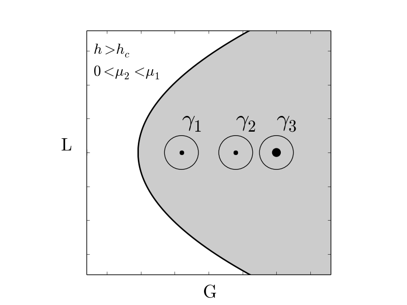
Figure 3. Energy slice of the bifurcation diagram for the spatial Euler problem, attractive case.

Let $\gamma_{i},i=1,2,3,$ be a simple closed curve in

$$NT_{h_{0}}=\{(h,g,l)\in NT\mid h=h_{0}\}$$

that encircles the critical line $\ell_{i}$, where

$$\ell_{1}=\{g=h+(\mu_{2}-\mu_{1}),\ l=0\},\ \ell_{2}=\{g=h+(\mu_{1}-\mu_{2}),\ l=0\}\ \mbox{ and }\ \\ \ell_{3}=\{g=h+(\mu_{1}+\mu_{2}),\ l=0\}.$$

For each $\gamma_{i}$, consider the torus bundle $F_{i}\colon E_{i}\to\gamma_{i}$, where the total space $E_{i}$ is obtained by gluing the ends of the fibers of $F$ over $\gamma_{i}$ via the scattering map $S$. We recall that scattering monodromy along $\gamma_{i}$ with respect to $H_{r}$ is defined as the usual monodromy of the torus bundle $F_{i}\colon E_{i}\to\gamma_{i}$; see Definition 5.6 and Appendix A.

Remark 6.3.

Alternatively, one can define $F_{i}\colon E_{i}\to\gamma_{i}$ by gluing the fibers of the original and the reference integral maps at infinity. Both definitions are equivalent in the sense that the monodromy of the resulting torus bundles are the same.

Consider a starting point $\gamma_{i}(t_{0})\in\gamma_{i}$ in the region where $l>0$. We choose a basis $(c_{\xi},c_{\eta},c_{\varphi})$ of the first homology group $\textup{H}_{1}(F_{i}^{-1}(\gamma_{i}(t_{0})))\simeq\mathbb{Z}^{3}$ as follows. The cycle $c_{\xi}=c^{o}_{\xi}\cup c^{r}_{\xi}$ is obtained by gluing the non-compact $\xi$-coordinate lines $c^{o}_{\xi}$ for the original and $c^{r}_{\xi}$ for the reference systems at infinity. In other words, for we glue the lines

$$p^{2}_{\xi}=\dfrac{(\xi^{2}-1)(2h\xi^{2}+2(\mu_{1}+\mu_{2})\xi-2g)-l^{2}}{(\xi^{2}-1)^{2}}$$

on $F^{-1}(\gamma_{i}(t_{0})),\gamma_{i}(t_{0})=(h,g,l)$, and

$$p^{2}_{\xi}=\dfrac{(\xi^{2}-1)(2h\xi^{2}+2(\mu_{2}-\mu_{1})\xi-2g)-l^{2}}{(\xi^{2}-1)^{2}}$$

on the reference fiber $F_{r}^{-1}(\gamma_{i}(t_{0}))$ at the limit points $\xi=\infty$, $p_{\xi}=\pm\sqrt{2h}.$ The cycles $c_{\eta}$ and $c_{\varphi}$ are such that their projections onto the configuration space coincide with coordinate lines of $\eta$ and $\varphi$, respectively. In other words, the cycle $c_{\eta}$ on $F^{-1}(\gamma_{i}(t_{0}))$ is given by

$$p^{2}_{\eta}=\dfrac{(1-\eta^{2})(-2h\eta^{2}-2(\mu_{1}-\mu_{2})\eta-2g)-l^{2}}{(1-\eta^{2})^{2}}$$

and $c_{\varphi}$ is an orbit of the circle action given by the Hamiltonian flow of the momentum $L_{z}$. We have the following result.

Theorem 6.4.

The monodromy matrices $M_{i}$ of $E_{i}\to\gamma_{i}$ with respect to the natural basis $(c_{\xi},c_{\eta},c_{\varphi})$ have the form

$$M_{1}=\begin{pmatrix}1&0&0\\ 0&1&1\\ 0&0&1\end{pmatrix},\ M_{2}=\begin{pmatrix}1&0&-1\\ 0&1&1\\ 0&0&1\end{pmatrix}\ \mbox{ and }\ M_{3}=\begin{pmatrix}1&0&1\\ 0&1&0\\ 0&0&1\end{pmatrix}.$$

Proof.

Case 1, loop $\gamma_{1}$. First we note that the cycle $c_{\varphi}$ is preserved under the parallel transport along $\gamma_{1}$. This follows from the fact that $L_{z}$ generates a free fiber-preserving circle action on $E_{i}$. The cycles $c_{\xi}$ and $c_{\eta}$ can be naturally transported only in the regions where $l\neq 0$. We thus need to understand what happens at the critical plane $l=0$.

Let $R>1$ be a sufficiently large number. Then

$$E_{1,R}=\{x\in E_{1}\mid\xi(x)>R\}$$

has exactly two connected components, which we denote by $E^{+}_{1,R}$ and $E^{-}_{1,R}$. We define a $1$-form $\alpha$ on (a part of) $E_{i}$ by the formula

$$\alpha=pdq-\chi(\xi)p_{\xi}(h,g,l,\xi)d\xi,$$

where $\chi(\xi)$ is a bump function such that

(i) $\chi(\xi)=0$ when $\xi<R;$

(ii) $\chi(\xi)=1$ when $\xi>1+R.$
The square root function $p_{\xi}(h,g,l,\xi)$ is assumed to be positive on $E^{+}_{1,R}$ and negative on $E^{-}_{1,R}$. By construction, the $1$-form $\alpha$ is well-defined and smooth on $E_{i}$ outside collision points. Since

$$d\alpha=dp\wedge dq=-\omega\ \mbox{ on }\ F^{-1}(\gamma_{i})\cup F_{r}^{-1}(\gamma_{i})\subset E_{i},$$

we have that $d\alpha=0$ on each fiber of $F_{i}$.

Consider the modified actions with respect to the form $\alpha$:

$$I_{\varphi}=\dfrac{1}{2\pi}\int\limits_{c_{\varphi}}\alpha,\ I_{\eta}=\dfrac{1}{2\pi}\int\limits_{c_{\eta}}\alpha\ \ \mbox{ and }\ \ I^{mod}_{\xi}=\dfrac{1}{2\pi}\int\limits_{c_{\xi}}\alpha.$$

The modified actions are well defined and, in view of $d\alpha=0$, depend only on the homology classes of $c_{\xi},c_{\eta}$ and $c_{\varphi}.$ It follows that $I_{\varphi}$ and $I_{\eta}$ coincide with the ‘natural’ actions (defined as the integrals over the usual $1$-form $pdq$). We note that the ‘natural’ $\xi$-action

$$I_{\xi}=\dfrac{1}{2\pi}\int\limits_{c_{\xi}}pdq$$

diverges, cf. [13]. From the continuity of the modified actions at $l=0$ it follows that the corresponding scattering monodromy matrix has the form

$$M_{1}=\begin{pmatrix}1&0&m_{1}\\ 0&1&m_{2}\\ 0&0&1\end{pmatrix}.$$

Since the modified actions do not have to be smooth at $l=0$, the integers $m_{1}$ and $m_{2}$ are not necessarily zero. In order to compute these integers we need to compare the derivatives $\partial_{l}I_{\eta}$ and $\partial_{l}I_{\xi}$ at $l\to\pm 0.$ A computation of the corresponding residues gives

$$\lim_{\l\to{\pm 0}}\partial_{l}I_{\eta}=\lim_{\l\to{\pm 0}}\dfrac{1}{2\pi}\partial_{l}\int\limits_{c_{\eta}}pdq=\begin{cases}0,&\mbox{ when }\ g<h+\mu_{2}-\mu_{1},\\ \mp 1/2,&\mbox{ when }\ \mu_{2}-\mu_{1}<g-h<\mu_{1}-\mu_{2},\end{cases}$$

and

$$\lim_{\l\to{\pm 0}}\partial_{l}I^{mod}_{\xi}=\lim_{\l\to{\pm 0}}\left(\dfrac{1}{2\pi}\partial_{l}\int\limits_{c^{o}_{\xi}}pdq-\dfrac{1}{2\pi}\partial_{l}\int\limits_{c^{r}_{\xi}}pdq\right)-\\ \lim_{\l\to{\pm 0}}\dfrac{1}{2\pi}\int\limits_{c_{\xi}}\chi(\xi)p_{\xi}(h,g,l,\xi)d\xi=0$$

(for the two ranges of $g$). It follows that $m_{1}=0$ and $m_{2}=1$.

Case 2, loop $\gamma_{2}$. This case is similar to Case 1. The corresponding limits are given by

$$\lim_{\l\to{\pm 0}}(\partial_{l}I_{\eta},\partial_{l}I^{mod}_{\xi})=\begin{cases}(\mp 1/2,0),&\mbox{ when }\ \mu_{2}-\mu_{1}<g-h<\mu_{1}-\mu_{2},\\ (\mp 1,\pm 1/2),&\mbox{ when }\ \mu_{1}-\mu_{2}<g-h<\mu_{1}+\mu_{1}.\end{cases}$$

Case 3, loop $\gamma_{3}$. The computation in this case is also similar to Case 1. The corresponding limits are given by

$$\lim_{\l\to{\pm 0}}(\partial_{l}I_{\eta},\partial_{l}I^{mod}_{\xi})=\begin{cases}(\mp 1,\pm 1/2),&\mbox{ when }\ \mu_{1}-\mu_{2}<g-h<\mu_{1}+\mu_{2},\\ (\mp 1,0),&\mbox{ when }\ h+\mu_{1}+\mu_{2}<g.\end{cases}$$

∎

Remark 6.5.

One difference between Case 3 and the other cases is the topology of the critical fiber, around which scattering monodromy is defined. In Case 3 the critical fiber is the product of a pinched cylinder and a circle, whereas in the other cases it is the product of a pinched torus and a real line. This implies, in fact, that Case 3 is purely scattering, whereas in the other cases Hamiltonian monodromy is present; see Subsection 6.3 for details.

Remark 6.6.

Theorem 6.4 admits the following geometric proof in the purely scattering case.

Proof for Case 3 of Theorem 6.4.

The action

$$I^{\prime}_{\eta}=\left.\begin{cases}I_{\eta},&\text{if }l\geq 0\\ I_{\eta}-2l,&\text{if }l<0.\end{cases}\right.$$

is smooth and globally defined (over $\gamma_{3}$). Moreover, the corresponding circle action extends to a free action in $F_{3}^{-1}(D_{3})$, where $D_{3}\subset NT_{h_{0}}$ is a $2$-disk such that $\partial D_{3}=\gamma_{3}$. Since there is also a circle action given by $I_{\varphi}$, the result can be also deduced from the general theory developed in [17, 38]. ∎

We note that from the last proof it follows that the choice of a reference Kepler Hamiltonian does not affect the result in the purely scattering case. This agrees with the point of view presented recently in [16] for two degree of freedom systems with focus-focus singularities. For the curves $\gamma_{1}$ and $\gamma_{2}$, it is important which of the two reference Kepler Hamiltonians is chosen; see Subsection 6.4.

As a corollary, we get the following result for the scattering map in the purely scattering case of the curve $\gamma_{3}$.

Theorem 6.7.

The scattering map $S\colon B_{3}\to B_{3},$ where $B_{3}=F^{-1}(\gamma_{3})/g^{t}_{H},$ is a Dehn twist. The push-forward map is conjugate in $SL(3,\mathbb{Z})$ to

$$S_{\star}=\begin{pmatrix}1&0&1\\ 0&1&0\\ 0&0&1\end{pmatrix}.$$

Proof.

The proof is similar to the proof of the equivalence $(2)\Leftrightarrow(3)$ given in Theorem 5.8. The scattering map $S$ allows one to consider the compactified torus bundle

$${\Pr}\colon{F^{-1}(\gamma_{3})}^{c}\to S^{1}=\mathbb{R}\cup\{\infty\},$$

where $\mathbb{R}$ corresponds to the time. The torus bundle $F_{3}\colon E_{3}\to\gamma_{3}$ has the same total space, but is fibered over $\gamma_{3}$. By Theorem 6.4, the monodromy of the bundle $F_{3}\colon E_{3}\to\gamma_{3}$ is given by the matrix

$$M=\begin{pmatrix}1&0&1\\ 0&1&0\\ 0&0&1\end{pmatrix}.$$

Then the monodromy of the first bundle ${\Pr}\colon{F^{-1}(\gamma_{3})}^{c}\to S^{1}$ is the same, for otherwise the total spaces would be different. The result follows. ∎

Remark 6.8.

It follows from the proof and Subsection 6.4 that Theorem 6.7 holds for any $\mu_{i}\neq 0$ and for any regular closed curve $\gamma\subset NT$ such that

1. The energy value $h$ is positive on $\gamma$;

2. $\gamma$ encircles the critical line $\{g=h+\mu_{1}+\mu_{2},\ l=0\}$ exactly once and does not encircle any other line of critical values;

3. $\gamma$ does not cross critical values of $F$.

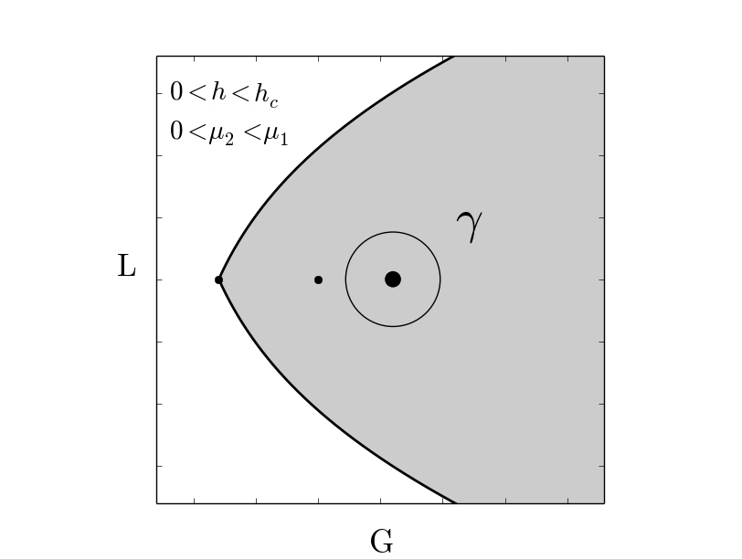
Figure 4. Energy slice of the bifurcation diagram for the spatial Euler problem, attractive case.

It can be shown that such a curve $\gamma$ always exists; an example is given in Fig. 4. We note that the third condition can be weakened in the case $-\mu_{1}<\mu_{2}<0$. In this case the attraction of $\mu_{1}$ dominates the repulsion of $\mu_{2}$ and, as a result, bound motion coexists with unbound motion for a range of positive energies. Instead of $F^{-1}(\gamma)$ one may consider its unbounded component.

6.3. Topology

As we have noted before, alongside scattering monodromy, the Euler problem admits also another type of invariant — Hamiltonian monodromy. Here we consider the generic case of $|\mu_{1}|\neq|\mu_{2}|\neq 0$ in the case of positive energies. The case of negative energies is similar — it has been discussed in detail in [51]. The critical cases can be easily computed from the generic case by considering curves that encircle more than one of the singular lines

$$\ell_{1}=\{g=h+(\mu_{2}-\mu_{1}),\ l=0\},\ \ell_{2}=\{g=h+(\mu_{1}-\mu_{2}),\ l=0\}\ \mbox{ and }\ \\ \ell_{3}=\{g=h+(\mu_{1}+\mu_{2}),\ l=0\}.$$

Let $\gamma_{i}$ be a closed curve that encircles only the critical line $\ell_{i}$; see Fig. 4. The fibration $F\colon F^{-1}(\gamma_{i})\to\gamma_{i}$ is a $T^{2}\times\mathbb{R}$-bundle. The following theorem shows that the Hamiltonian monodromy (see Appendix A) is non-trivial along the curves $\gamma_{1}$ and $\gamma_{2}$ and is trivial along $\gamma_{3}$.

Theorem 6.9.

The Hamiltonian monodromy of $F\colon F^{-1}(\gamma_{i})\to\gamma_{i},\ i=1,2$, is conjugate in $SL(2,\mathbb{Z})\subset SL(3,\mathbb{Z})$ to

$$M=\begin{pmatrix}1&0&0\\ 0&1&1\\ 0&0&1\end{pmatrix}.$$

Here the right-bottom $2\times 2$ block acts on $T^{2}$ and the left-top $1\times 1$ block acts on $\mathbb{R}$.

Proof.

The result follows from the proof of Theorem 6.4. For completeness, we give an independent proof below.

After the reduction of the surface $H^{-1}(h)$ with respect to the flow $g^{t}_{H}$ we get a singular $T^{2}$ torus fibration over a disk $D_{i},\ \partial D_{i}=\gamma_{i},$ with exactly one focus-focus point. The result then follows from [37, 41, 54]. This argument applies to both of the lines $\ell_{1}$ and $\ell_{2}$. Since the flow of $L_{z}$ gives a global circle action, the monodromy matrix $M$ is the same in both cases; see [9]. ∎

Theorem 6.10.

The Hamiltonian monodromy of $F\colon F^{-1}(\gamma_{3})\to\gamma_{3}$ is trivial.

Proof.

Observe that the Hamiltonian flows of $I_{\varphi},$

$$I^{\prime}_{\eta}=\left.\begin{cases}I_{\eta},&\text{if }l\geq 0\\ I_{\eta}-2l,&\text{if }l<0.\end{cases}\right.$$

and $H$ generate a global $\mathbb{T}^{2}\times\mathbb{R}$ action on $F^{-1}(\gamma_{3})$. It follows that the bundle $F\colon F^{-1}(\gamma_{3})\to\gamma_{3}$ is principal. Since $\gamma_{3}$ is a circle, it is also trivial. ∎

We note that Hamiltonian monodromy is an intrinsic invariant of the Euler problem, related to the non-trivial topology of the integral map $F$. Interestingly, it is also present in the critical cases:

(1) $\mu_{1}=\mu_{2}$ (symmetric Euler problem) [51],

(2) $\mu_{1}$ or $\mu_{2}=0$ (Kepler problem) [15] and

(3) $\mu_{1}=\mu_{2}=0$ (the free flow).
In the case of bound motion (1) and (2) are due to [51] and [15], respectively. From the scattering perspective Hamiltonian monodromy is recovered if one considers the original Hamiltonian $H$ also as a reference.

6.4. General case

Here we consider the case of of arbitrary strengths $\mu_{i}$. We observe that the scattering monodromy matrices with respect to the reference Kepler Hamiltonians $H_{r_{1}}$ and $H_{r_{2}}$ are necessarily of the form

$$\left(\begin{array}[]{ccc}1&0&m\\ 0&1&n\\ 0&0&1\end{array}\right)$$

for some integers $m$ and $n$. These integers (for different choices of the strengths $\mu_{i}$ and the critical lines $\ell_{i}$) are given in Table 1.

Remark 6.11.

We note that one can compute the monodromy matrices in the critical cases from the matrices found in the generic cases. Specifically, it is sufficient to consider the curves that encircle more than one critical line $\ell_{i}$ and multiply the monodromy matrices found around each of these lines. For instance, the monodromy matrix around the curve $g=h$ in the free flow equals the product of the three monodromy matrices found in (any) generic Euler problem.

	$\gamma_{1}$	$\gamma_{2}$	$\gamma_{3}$
	Scattering monodromy w.r.t. $H_{r_{1}}$
Generic
$|\mu_{1}|\neq|\mu_{2}|\neq 0$	$m=-1,n=1$	$m=0,n=1$	$m=1,n=0$
Critical
$-\mu_{1}=\mu_{2}<0$	$m=-1,n=1$	$m=0,n=1$	$n=1,n=0$
$0<\mu_{1}=\mu_{2}$	$m=-1,n=2$		$m=1,n=0$
$\mu_{1}=\mu_{2}<0$	$m=-1,n=2$		$m=1,n=0$
$\mu_{1}=\mu_{2}=0$	$m=0,n=2$
$0=\mu_{2}<\mu_{1}$	$n=1$	$m=0,n=1$	$\ \ \ \ \ \ \ \ \ \ \ \ m=0,$
$\mu_{1}<\mu_{2}=0$	$m=-1,n=1$	$m=1,n=1$
	Scattering monodromy w.r.t. $H_{r_{2}}$
Generic
$|\mu_{1}|\neq|\mu_{2}|\neq 0$	$m=0,n=1$	$m=-1,n=1$	$m=1,n=0$
Critical
$-\mu_{1}=\mu_{2}<0$	$m=0,n=1$	$m=-1,n=1$	$m=1,n=0$
$0=\mu_{2}<\mu_{1}$	$n=1$	$m=-1,n=1$	$\ \ \ \ \ \ \ \ \ \ \ \ m=1,$
$\mu_{1}<\mu_{2}=0$	$m=0,n=1$	$m=0,n=1$

Table 1. Scattering monodromy, general case.

7. Discussion

In the present paper we have shown that the spatial Euler problem, alongside non-trivial Hamiltonian monodromy [51], has non-trivial scattering monodromy of two different types: pure and mixed scattering monodromy. The first type reflects the presence of a special periodic orbit — a collision orbit that bounces between the two centers — and the associated trapping trajectories. In the spatial case one can go around these trajectories and compare the flow at infinity to an appropriately chosen Kepler problem. Scattering monodromy of the second type is related to the difference in dynamics of the original and the reference systems; here in addition to scattering monodromy also Hamiltonian monodromy is present. Interestingly, scattering monodromy of the second type survives vanishing of one of the centers: it can be also observed in the limiting case of attractive and repulsive Kepler problems

$$H_{r_{1}}=\frac{1}{2}p^{2}-\dfrac{\mu}{r_{1}}\ \mbox{ and }\ H_{r_{2}}=\frac{1}{2}p^{2}+\dfrac{\mu}{r_{2}}.$$

Hamiltonian monodromy is present not only in the Kepler problem [15], but also in the free flow. The purely scattering monodromy is special to the genuine Euler problem; we conjecture that this invariant is also present in the restricted three-body problem.

8. Acknowledgements

We would like to thank Prof. Dr. A. Knauf for the useful and stimulating discussions.

Appendix A Hamiltonian monodromy

Consider an integrable Hamiltonian system $F=(F_{1}=H,F_{2},\ldots,F_{n})$ on a $2n$-dimensional symplectic manifold $(M,\omega)$. If the fibers of the integral map $F$ are compact and connected, then according to the classical Arnol’d-Liouville theorem [1] a tubular neighborhood of each regular fiber is a trivial torus bundle $D^{n}\times T^{n}$ admitting action-angle coordinates. Hence

$$F\colon F^{-1}(R)\to R,$$

where $R\subset\textup{image}(F)$ is the set of regular values of $F$, is a locally trivial torus bundle. This bundle is, however, not necessary globally trivial even from the topological viewpoint. One geometric invariant that measures this non-triviality was introduced by Duistermaat in [12] and is called Hamiltonian monodromy. Specifically, Hamiltonian monodromy is defined as a representation

$$\pi_{1}(R,\xi_{0})\to\textup{Aut}\,H_{1}(F^{-1}(\xi_{0}))\simeq\mathrm{GL}(n,\mathbb{Z})$$

of the fundamental group $\pi_{1}(R,\xi_{0})$ in the group of automorphisms of the integer homology group $H_{1}(F^{-1}(\xi_{0}))\simeq\mathbb{Z}^{n}$. Each element $\gamma\in\pi_{1}(R,\xi_{0})$ acts via parallel transport of integer homology cycles [12].

Since the pioneering work of Duistermaat, Hamiltonian monodromy and its quantum counterpart [7, 49] have been observed in many integrable systems of physics and mechanics. General results are known that allow to compute this invariant in specific examples. It has been shown in [37, 41, 54] that in the typical case of $n=2$ degrees of freedom non-trivial Hamiltonian monodromy is manifested by the presence of the so-called focus-focus points of the map $F$. In the case of a global circle action Hamiltonian monodromy (and, more generally, fractional monodromy [42]) can be computed in terms of the singularities of the circle action [17, 38].

Remark A.1.

A notion of monodromy can be defined for torus bundles that do not necessarily come from an integrable system and also in the case of bundles with non-compact fibers (for instance, in the case of cylinder bundles). Specifically, consider a bundle $F\colon F^{-1}(\gamma)\to\gamma,\ \gamma=S^{1}.$ It can be obtained from a direct product $[0,1]\times F^{-1}(\gamma(t_{0}))$ by gluing the boundaries via a non-trivial homeomorphism $f$, called the monodromy of the bundle. We call this monodromy Hamiltonian if $F$ comes from a completely integrable system. In this case the push-forward map $f_{\star}$ coincides with the automorphism given by the parallel transport.

We note that non-compact fibrations appear in the Euler problem in the case of positive energies and in various other integrable systems. We mention the works [22, 35, 40] and [2, 13, 53, 16]. For systems that are both scattering and integrable scattering monodromy and Hamiltonian monodromy coincide if the reference is given by the original Hamiltonian $H$.

Appendix B Bifurcation diagrams for the planar problem

In this section we give bifurcation diagrams of the planar Euler problem in the case of arbitrary strengths $\mu_{i}$. The computation has been performed in Section 3; more details can be found in [10, 51, 46].

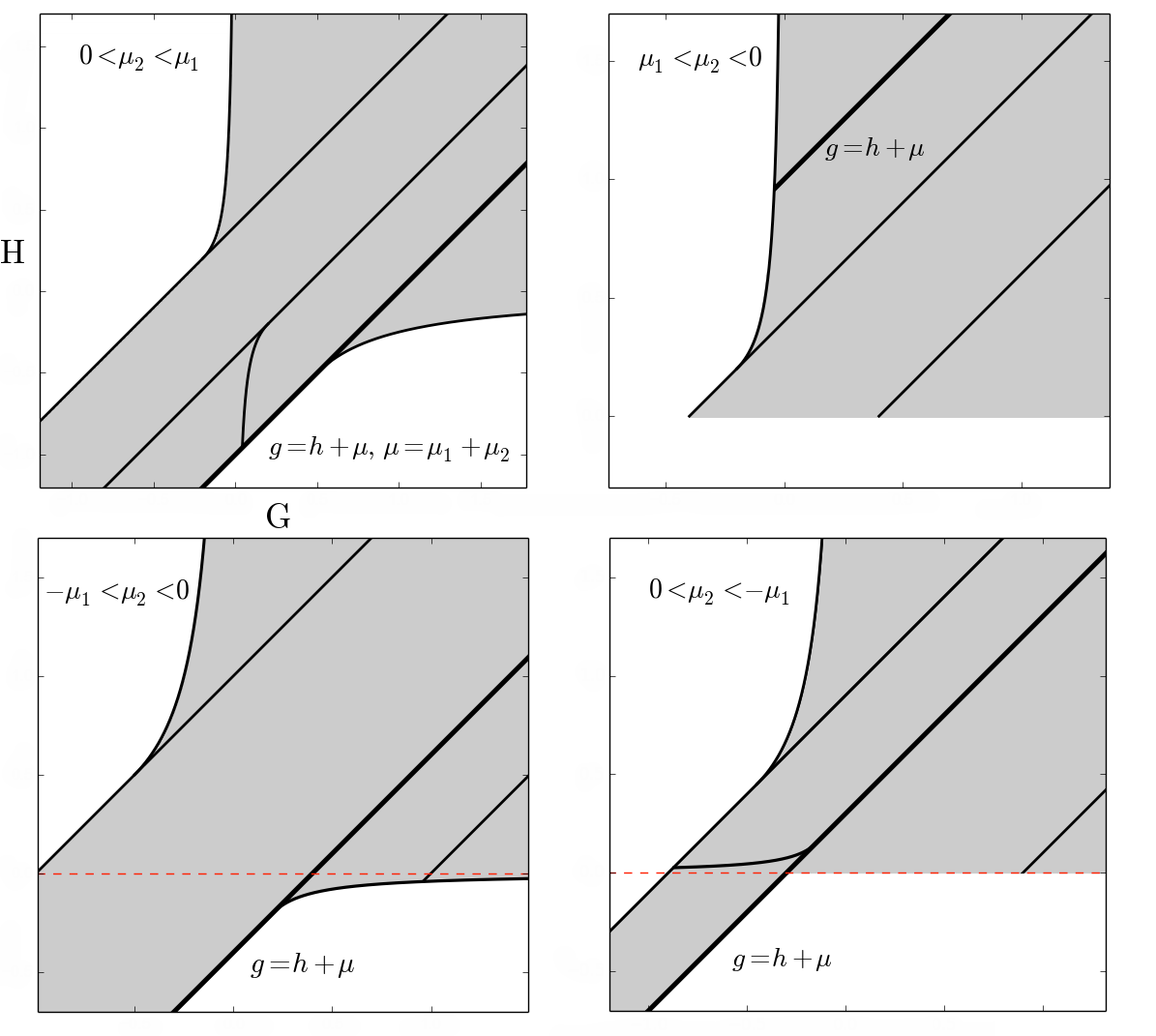
Figure 5. Bifurcation diagrams for the planar problem, generic cases $|\mu_{1}|\neq|\mu_{2}|\neq 0$. Top: attractive (left), repulsive (right). Bottom: mixed.

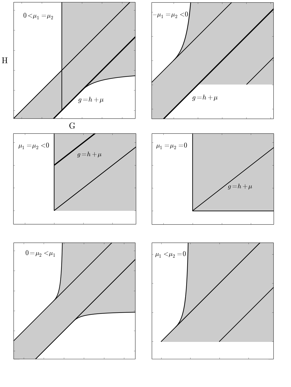
Figure 6. Bifurcation diagrams for the planar problem, non-generic cases $|\mu_{1}|=|\mu_{2}|$ or $\mu_{1}\mu_{2}=0$. From left to right, from top to bottom: symmetric attractive, anti-symmetric, symmetric repulsive, free flow, attractive Kepler problem, repulsive Kepler problem.

The computation of Section 3 yields the following critical lines

(8) $$\ell_{1}=\{g=h+\mu_{2}-\mu_{1}\},\ \ell_{2}=\{g=h+\mu_{1}-\mu_{2}\}\\ \mbox{ and }\ \ell_{3}=\{g=h+\mu\},\ \mu=\mu_{1}+\mu_{2},$$

and the critical curves

$$\{g =\mu\cosh\lambda/2,\ h=-\mu/2\cosh\lambda\},$$

$$\{g =(\mu_{1}-\mu_{2})\sin\nu/2,\ h=(\mu_{2}-\mu_{1})/2\sin\nu\}.$$

Points that do not correspond to any physical motion must be removed from the obtained set. The resulting diagrams are given in Figs. 5 and 6. Here we distinguish two cases: generic case when the strengths $|\mu_{1}|\neq|\mu_{2}|\neq 0$ and the remaining critical cases.

We note that the critical cases occur when $|\mu_{1}|=|\mu_{2}|$ or when $\mu_{1}\mu_{2}=0$. In the case $\mu_{1}=-\mu_{2}\neq 0$ the attraction of one of the centers equalizes the repulsion of the other center, making the bifurcation diagram qualitatively different from the cases when $-\mu_{1}<\mu_{2}<0$ or $0<\mu_{2}<-\mu_{1}$. However, we still have the three different critical lines $\ell_{1},\ell_{2}$ and $\ell_{3}$. In the other critical cases collisions of the critical lines $\ell_{i}$ occur. For instance, $\mu_{1}=0$ implies that $\ell_{1}=\ell_{3}$ and so on. The same situation takes place in the spatial problem.

Appendix C Proof of Theorem 5.4

We shall show that the Euler problem has two natural reference Hamiltonians when $\mu_{1}\neq\mu_{2}$ and one otherwise.

Theorem C.1.

Among all Kepler Hamiltonians only

$$H_{r_{1}}=\frac{1}{2}p^{2}-\dfrac{\mu_{1}-\mu_{2}}{r_{1}}\ \mbox{ and }\ H_{r_{2}}=\frac{1}{2}p^{2}-\dfrac{\mu_{2}-\mu_{1}}{r_{2}}$$

are reference Hamiltonians of $F=(H,L_{z},G)$. In particular, the free Hamiltonian is a reference Hamiltonian of $F$ only in the case $\mu_{1}=\mu_{2}$.

Proof.

Sufficiency. Consider the Hamiltonian $H_{r_{1}}$. Let

$$G_{r_{1}}=H_{r_{1}}+\frac{1}{2}(L^{2}-a^{2}(p_{x}^{2}+p_{y}^{2}))+a(z+a)\frac{\mu_{1}-\mu_{2}}{r_{1}}.$$

From Section 2.1 (see also Eq. (3)) it follows that the functions $H_{r_{1}},L_{z}$ and $G_{r_{1}}$ Poisson commute. This implies that any trajectory $g^{t}_{H_{r_{1}}}(x)$ belongs to the common level set of $F_{r_{1}}=(H_{r_{1}},L_{z},G_{r_{1}}).$ For a scattering trajectory we thus get

$$F_{r_{1}}\left(\lim\limits_{t\to+\infty}g^{t}_{H_{r_{1}}}(x)\right)=F_{r_{1}}\left(\lim\limits_{t\to-\infty}g^{t}_{H_{r_{1}}}(x)\right).$$

A straightforward computation of the limit shows that also

$$F\left(\lim\limits_{t\to+\infty}g^{t}_{H_{r_{1}}}(x)\right)=F\left(\lim\limits_{t\to-\infty}g^{t}_{H_{r_{1}}}(x)\right).$$

The case of $H_{r_{2}}$ is completely analogous.

Figure 7. Kepler trajectory $g^{t}_{H_{r}}(x)$ in the $z=z_{0}$ plane.

Necessity. Without loss of generality $\mu_{2}\leq\mu_{1}$. Let

$$H_{r}=\frac{1}{2}p^{2}-\dfrac{\mu}{r},$$

where $r\colon\mathbb{R}^{3}\setminus\{o\}\to\mathbb{R}$ is the distance to some point $o\in\mathbb{R}^{3}$, be a reference Hamiltonian of $F$. We have to show that

• $\mu>0$ implies $o=o_{1}$ and $\mu=\mu_{1}-\mu_{2}$;

• $\mu<0$ implies $o=o_{2}$ and $\mu=\mu_{2}-\mu_{1}$;

• $\mu=0$ implies $\mu_{1}=\mu_{2}$.

Case 1. First we show that $o$ belongs to the $z$ axis. If this is not the case, then, due to rotational symmetry, we have a reference Hamiltonian $H_{r}$ with $o=(-b_{0},0,z_{0})$ for some $b_{0},\ z_{0}\in\mathbb{R},\ b_{0}\neq 0$. This reference Hamiltonian $H_{r}$ has a trajectory $t\mapsto g^{t}_{H_{r}}(x)$ that (in the configuration space) has the form shown in Figure 7. But for such a trajectory

$$L_{z}\left(\lim\limits_{t\to+\infty}g^{t}_{H_{r_{1}}}(x)\right)=0\neq\sqrt{2h}\cdot b_{0}=L_{z}\left(\lim\limits_{t\to-\infty}g^{t}_{H_{r_{1}}}(x)\right),$$

where $h=H_{r}(x)>0$ is the energy of $g^{t}_{H_{r}}(x)$. We conclude that $o=(0,0,b)$ for some $b\in\mathbb{R}$.

Next we show that $b\mu=a(\mu_{1}-\mu_{2})$. Consider a trajectory $g^{t}_{H_{r}}(x)$ of $H_{r}$ that has the form shown in Figure 8$a$.

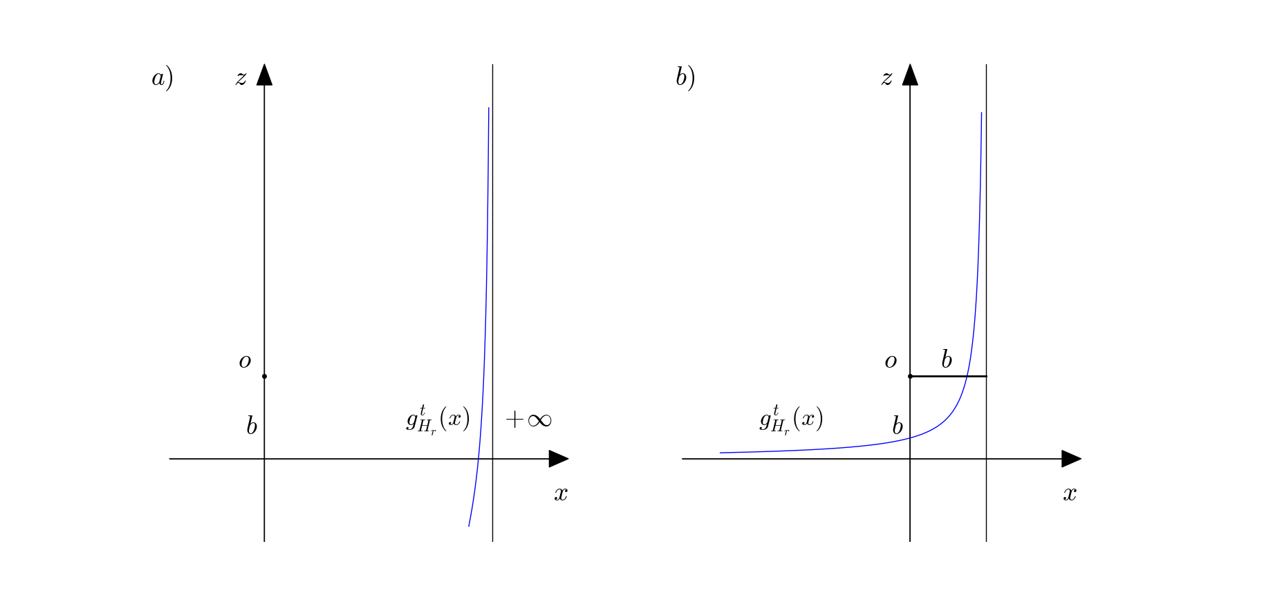
Figure 8. Kepler trajectories in the $y=0$ plane.

It follows from Eq. (3) that the function

$$G_{r}=H_{r}+\frac{1}{2}(L^{2}-b^{2}(p_{x}^{2}+p_{y}^{2}))+b(z+b)\frac{\mu}{r}$$

is constant along this trajectory. Thus, for $H_{r}$ to be a reference Hamiltonian we must have

(9) $$(G-G_{r})\left(\lim\limits_{t\to+\infty}g^{t}_{H_{r_{1}}}(x)\right)=(G-G_{r})\left(\lim\limits_{t\to-\infty}g^{t}_{H_{r_{1}}}(x)\right).$$

In the configuration space, $g^{t}_{H_{r}}(x)$ is asymptotic to the ray $x=c,\ y=0,\ z\geq 0$ at $t=+\infty$. The other asymptote at $t=-\infty$ gets arbitrarily close to the ray $x=c,\ y=0,\ z\leq 0$ when $c\to+\infty$. It follows that Eq. (9) is equivalent to

$$a(\mu_{1}-\mu_{2})-b\mu=b\mu-a(\mu_{1}-\mu_{2})+\varepsilon,$$

where $\varepsilon\to 0$ when $c\to+\infty$.

The remaining equality $b=a$ can be proven using a trajectory $g^{t}_{H_{r}}(x)$ that has the form shown in Figure 8$b$.

Case 2. In this case trajectories $g^{t}_{H_{r}}(x)$ of the repulsive Kepler Hamiltonian $H_{r}$ do not project to the curves shown in Figs. 7, 8$a$ and 8$b$. However, each of these curves is a branch of a hyperbola. The ‘complementary’ branches are (projections of) trajectories of $H_{r}$; see Fig. 9. If the latter branches are used, the proof becomes similar to Case 1.

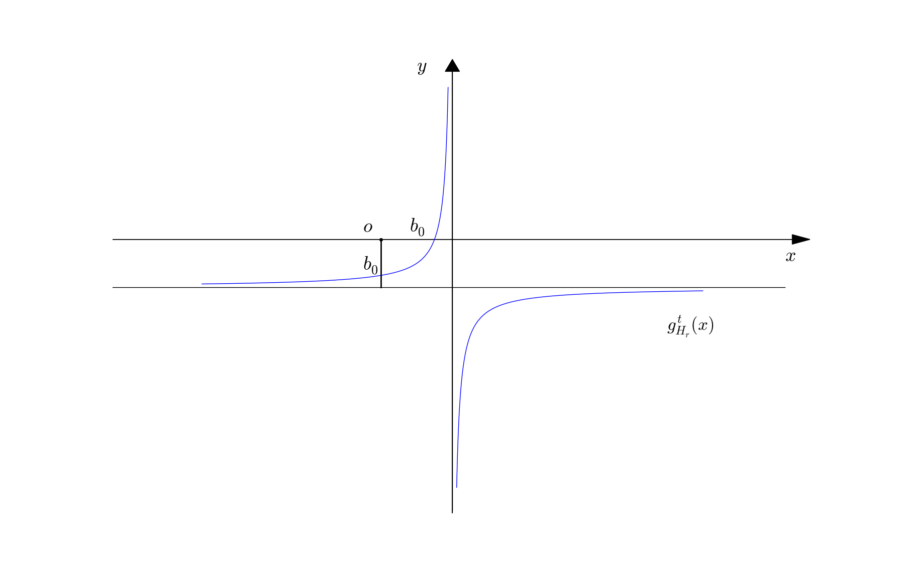
Figure 9. The two branches ($z=z_{0}$ plane). In the repulsive case $\mu>0$ a Kepler trajectory is represented by the convex branch.

Case 3. In this case $H_{r}$ generates the free motion. Let

$$g^{t}_{H_{r}}(x)=(q(t),p(t)),\ q(t)=(c,0,t),\ p(t)=(0,0,1).$$

Since $L^{2}$ and $(p_{x},p_{y},p_{z})$ are conserved,

$$G\left(\lim\limits_{t\to+\infty}g^{t}_{H_{r_{1}}}(x)\right)=G\left(\lim\limits_{t\to-\infty}g^{t}_{H_{r_{1}}}(x)\right)$$

implies $a(\mu_{1}-\mu_{2})=a(\mu_{2}-\mu_{1})$ and hence $\mu_{1}=\mu_{2}$. ∎

References

- [1] V.I. Arnol’d and A. Avez, Ergodic problems of classical mechanics, W.A. Benjamin, Inc., 1968.
- [2] L. Bates and R. Cushman, Scattering monodromy and the A1 singularity, Central European Journal of Mathematics 5 (2007), no. 3, 429–451.
- [3] A.V. Bolsinov and A.T. Fomenko, Integrable Hamiltonian Systems: Geometry, Topology, Classification, CRC Press, 2004.
- [4] A.V. Bolsinov, S.V. Matveev, and Fomenko A.T., Topological classification of integrable Hamiltonian systems with two degrees of freedom. list of systems of small complexity, Russian Mathematical Surveys 45 (1990), no. 2, 59.
- [5] C.L. Charlier, Die Mechanik des Himmels, Veit and Comp, 1902.
- [6] J.M. Cook, Banach algebras and asymptotic mechanics, Application of Mathematics to Problems in Theoretical Physics: Proceedings, Summer School of Theoretical Physics, vol. 6, 1967, pp. 209–246.
- [7] R. Cushman and J.J. Duistermaat, The quantum mechanical spherical pendulum, Bulletin of the American Mathematical Society 19 (1988), no. 2, 475–479.
- [8] R.H. Cushman and L.M. Bates, Global aspects of classical integrable systems, 2 ed., Birkhäuser, 2015.
- [9] R.H. Cushman and S. Vũ Ngọc, Sign of the monodromy for Liouville integrable systems, Annales Henri Poincaré 3 (2002), no. 5, 883–894.
- [10] A. Deprit, Le problème des deux centres fixes, Bull. Soc. Math. Belg 14 (1962), no. 11, 12–45.
- [11] J. Derezinski and C. Gerard, Scattering theory of classical and quantum n-particle systems, Theoretical and Mathematical Physics, Springer Berlin Heidelberg, 2013.
- [12] J. J. Duistermaat, On global action-angle coordinates, Communications on Pure and Applied Mathematics 33 (1980), no. 6, 687–706.
- [13] H. Dullin and H. Waalkens, Nonuniqueness of the phase shift in central scattering due to monodromy, Phys. Rev. Lett. 101 (2008).
- [14] H. R. Dullin and R. Montgomery, Syzygies in the two center problem, Nonlinearity 29 (2016), no. 4, 1212.
- [15] Holger R. Dullin and Holger Waalkens, Defect in the joint spectrum of hydrogen due to monodromy, Phys. Rev. Lett. 120 (2018), 020507.
- [16] K. Efstathiou, A. Giacobbe, P. Mardešić, and D. Sugny, Rotation forms and local Hamiltonian monodromy, Submitted (2016).
- [17] K. Efstathiou and N. Martynchuk, Monodromy of Hamiltonian systems with complexity-1 torus actions, Geometry and Physics 115 (2017), 104–115.
- [18] H.A. Erikson and E.L. Hill, A note on the one-electron states of diatomic molecules, Phys. Rev. 75 (1949), 29–31.
- [19] L. Euler, Probleme. Un corps étant attiré en raison réciproque quarrée des distances vers deux points fixes donnés, trouver les cas où la courbe décrite par ce corps sera algébrique, Histoire de L’Académie Royale des sciences et Belles-lettres XVI ((1760), 1767), 228–249.
- [20] by same author, De motu corporis ad duo centra virium fixa attracti, Novi Commentarii academiae scientiarum Petropolitanae 10 (1766), 207–242.
- [21] by same author, De motu corporis ad duo centra virium fixa attracti, Novi Commentarii academiae scientiarum Petropolitanae 11 (1767), 152–184.
- [22] H. Flaschka, A remark on integrable Hamiltonian systems, Physics Letters A 131 (1988), no. 9, 505 – 508.
- [23] A.T. Fomenko, Morse theory of integrable Hamiltonian systems, Dokl. Akad. Nauk SSSR, vol. 287, 1986, pp. 1071–1075.
- [24] by same author, The topology of surfaces of constant energy in integrable Hamiltonian systems, and obstructions to integrability, Izvestiya: Mathematics 29 (1987), no. 3, 629–658.
- [25] A.T. Fomenko and H. Zieschang, Topological invariant and a criterion for equivalence of integrable Hamiltonian systems with two degrees of freedom, Izv. Akad. Nauk SSSR, Ser. Mat. 54 (1990), no. 3, 546–575 (Russian).
- [26] I. A. Gerasimov, Euler problem of two fixed centers, Friazino, (2007), (in Russian).
- [27] I.W. Herbst, Classical scattering with long range forces, Comm. Math. Phys. 35 (1974), no. 3, 193–214.
- [28] W. Hunziker, The S-matrix in classical mechanics, Comm. Math. Phys. 8 (1968), no. 4, 282–299.
- [29] C̃. G. J. Jacobi, Vorlesungen über Dynamik, Chelsea Publ., New York, 1884.
- [30] S. Kim, Homoclinic orbits in the Euler problem of two fixed centers, https://arxiv.org/abs/1606.05622 (2017).
- [31] M. Klein and A. Knauf, Classical Planar Scattering by Coulombic Potentials, Lecture Notes in Physics Monographs, Springer Berlin Heidelberg, 2008.
- [32] A. Knauf, Qualitative aspects of classical potential scattering, Regul. Chaotic Dyn. 4 (1999), no. 1, 3–22.
- [33] by same author, Mathematische Physik, Springer-Lehrbuch Masterclass, Springer Berlin Heidelberg, 2011.
- [34] A. Knauf and M. Krapf, The non-trapping degree of scattering, Nonlinearity 21 (2008), no. 9, 2023.
- [35] E.A. Kudryavtseva and T.A. Lepskii, The topology of Lagrangian foliations of integrable systems with hyperelliptic Hamiltonian, Sbornik: Mathematics 202 (2011), no. 3, 373.
- [36] J.L. Lagrange, Miscellania taurinensia, Recherches sur la mouvement d’un corps qui est attiré vers deux centres fixes 14 (1766-69).
- [37] L.M. Lerman and Ya.L. Umanskiĭ, Classification of four-dimensional integrable Hamiltonian systems and Poisson actions of in extended neighborhoods of simple singular points. i, Russian Academy of Sciences. Sbornik Mathematics 77 (1994), no. 2, 511–542.
- [38] N. Martynchuk and K. Efstathiou, Parallel transport along Seifert manifolds and fractional monodromy, Communications in Mathematical Physics 356 (2017), no. 2, 427–449.
- [39] N. Martynchuk and H. Waalkens, Knauf’s degree and monodromy in planar potential scattering, Regular and Chaotic Dynamics 21 (2016), no. 6, 697–706.
- [40] N.N. Martynchuk, Semi-local Liouville equivalence of complex Hamiltonian systems defined by rational Hamiltonian, Topology and its Applications 191 (2015), no. Supplement C, 119 – 130.
- [41] V.S. Matveev, Integrable Hamiltonian system with two degrees of freedom. The topological structure of saturated neighbourhoods of points of focus-focus and saddle-saddle type, Sbornik: Mathematics 187 (1996), no. 4, 495–524.
- [42] N.N. Nekhoroshev, D.A. Sadovskií, and B.I. Zhilinskií, Fractional Hamiltonian monodromy, Annales Henri Poincaré 7 (2006), 1099–1211.
- [43] K.F. Niessen, Zur Quantentheorie des Wasserstoffmolekülions, Annalen der Physik 375 (1923), no. 2, 129–134.
- [44] D. Ó’Mathúna, Integrable systems in celestial mechanics, Birkhäuser, Basel, 2008.
- [45] W. Pauli, Über das Modell des Wasserstoffmolekülions, Annalen der Physik 373 (1922), no. 11, 177–240.
- [46] M. Seri, The problem of two fixed centers: bifurcation diagram for positive energies, Journal of Mathematical Physics 56 (2015), no. 1, 012902.
- [47] M. Seri, A. Knauf, M. D. Esposti, and T. Jecko, Resonances in the two-center Coulomb systems, Reviews in Mathematical Physics 28 (2016), no. 07, 1650016.
- [48] B. Simon, Wave operators for classical particle scattering, Comm. Math. Phys. 23 (1971), no. 1, 37–48.
- [49] S. Vũ Ngọc, Quantum monodromy in integrable systems, Communications in Mathematical Physics 203 (1999), no. 2, 465–479.
- [50] T.G. Vosmischera, Integrable systems of celestial mechanics in space of constant curvature, Springer Netherlands, 2003.
- [51] H. Waalkens, H.R. Dullin, and P.H. Richter, The problem of two fixed centers: bifurcations, actions, monodromy, Physica D 196 (2004), no. 3-4, 265–310.
- [52] E.T. Whittaker, A treatise on the analytical dynamics of particles and rigid bodies; with an introduction to the problem of three bodies, Cambridge, University Press, 1917.
- [53] O.A. Zagryadskii, E.A. Kudryavtseva, and D.A. Fedoseev, A generalization of Bertrand’s theorem to surfaces of revolution, Sbornik: Mathematics 203 (2012), no. 8, 1112.
- [54] N.T. Zung, A note on focus-focus singularities, Differential Geometry and its Applications 7 (1997), no. 2, 123–130.