A randomized and fully discrete
Galerkin finite element method for
semilinear stochastic evolution equations

Abstract.

In this paper the numerical solution of non-autonomous semilinear stochastic evolution equations driven by an additive Wiener noise is investigated. We introduce a novel fully discrete numerical approximation that combines a standard Galerkin finite element method with a randomized Runge–Kutta scheme. Convergence of the method to the mild solution is proven with respect to the $L^{p}$-norm, $p\in[2,\infty)$. We obtain the same temporal order of convergence as for Milstein–Galerkin finite element methods but without imposing any differentiability condition on the nonlinearity. The results are extended to also incorporate a spectral approximation of the driving Wiener process. An application to a stochastic partial differential equation is discussed and illustrated through a numerical experiment.

1. Introduction

In this paper we investigate the numerical solution of non-autonomous semilinear stochastic evolution equations (SEE) driven by an additive Wiener noise. More precisely, let $(H,(\cdot,\cdot),\|\cdot\|)$ and $(U,(\cdot,\cdot)_{U},\|\cdot\|_{U})$ be two separable ${\mathbb{R}}$-Hilbert spaces. For a given $T\in(0,\infty)$ we denote by $(\Omega_{W},{\mathcal{F}}^{W},({\mathcal{F}}^{W}_{t})_{t\in[0,T]},{\mathbb{P}}_{W})$ a filtered probability space satisfying the usual conditions. By $(W(t))_{t\in[0,T]}$ we denote a cylindrical $({\mathcal{F}}^{W}_{t})_{t\in[0,T]}$-Wiener process on $U$ with associated covariance operator $Q\in\mathcal{L}(U)$.

Our goal is the approximation of the mild solution to SEEs of the form

(1) $$\begin{cases}\,\mathrm{d}X(t)+\big{[}AX(t)+f(t,X(t))\big{]}\,\mathrm{d}t=g(t)\,\mathrm{d}W(t),&\quad\text{for }t\in(0,T],\\ X(0)=X_{0}.&\end{cases}$$

Hereby, we assume that $-A\colon{\mathrm{dom}}(A)\subset H\to H$ is the infinitesimal generator of an analytic semigroup $(S(t))_{t\in[0,\infty)}\subset\mathcal{L}(H)$ on $H$. The initial value $X_{0}\colon\Omega_{W}\to H$ is assumed to be a $p$-fold integrable random variable for some $p\in[2,\infty)$, while the mapping $g\colon[0,T]\to\mathcal{L}_{2}^{0}$ is Hölder continuous with exponent $\frac{1}{2}$. Here $\mathcal{L}_{2}^{0}=\mathcal{L}_{2}(Q^{\frac{1}{2}}(U),H)$ denotes the set of all Hilbert–Schmidt operators from $Q^{\frac{1}{2}}(U)$ to $H$. In addition, the mapping $f$ is assumed to be Lipschitz continuous. A complete and more precise statement of all conditions on $A$, $f$, $g$, and $X_{0}$ is given in Section 3.

Under these assumptions the mild solution $X\colon[0,T]\times\Omega_{W}\to H$ to (1) is uniquely determined by the variation-of-constants formula

(2) $$X(t)=S(t)X_{0}-\int_{0}^{t}S(t-s)f(s,X(s))\,\mathrm{d}s+\int_{0}^{t}S(t-s)g(s)\,\mathrm{d}W(s)$$

which holds ${\mathbb{P}}_{W}$-almost surely for all $t\in[0,T]$. Our assumptions in Section 3 ensure the existence of a unique mild solution to (1). We refer the reader to [7] for a general introduction of the semigroup approach to stochastic evolution equations. We also refer to [27, Chapter 2] for further details on cylindrical Wiener processes and Hilbert space valued stochastic integrals.

Due to the presence of the noise the mild solution is, in general, only of very low spatial and temporal regularity. This in turn results in low convergence rates of numerical approximations. Examples for standard numerical methods for SEEs are found, for instance, in the monographs [16, 19, 24] and the references therein. Because of this, an accurate simulation of stochastic evolution equations is often computationally expensive. This explains why the development of strategies to reduce the computational complexity has attracted a lot of attention over the last decade. In particular, we mention the multilevel Monte-Carlo method that has been applied to stochastic partial differential equations, for instance, in [3]. However, the success of this approach depends on the availability of efficient numerical methods which converge with a high order with respect to the mean-square norm.

One way to construct such higher order numerical approximations is based on Itō–Taylor expansions as discussed in [16]. In fact, provided the coefficient functions are sufficiently smooth, numerical methods of basically any temporal order can be constructed. However, these methods sometimes behave unstable in numerical simulations and the necessity to evaluate higher order derivatives or to generate multiple iterated stochastic integrals limits their practical relevance. More severely, already the imposed smoothness requirements are too restrictive in most applications of SEEs in infinite dimensions. For instance, the general assumption in [16, Chapter 8] asks for the semilinearity $f\colon[0,T]\times H\to H$ to be infinitely often Fréchet differentiable with bounded derivatives. This condition already excludes any truly nonlinear Nemytskii-type operator. Compare further with Remark 3.8 below. We also refer to [1, 2, 4, 17, 18, 23, 34] for further numerical methods with a higher order temporal convergence rate, such as Milstein-type schemes or Wagner–Platen-type methods. Although the smoothness conditions on $f$ are substantially relaxed in some of these papers, all results at least require the Fréchet differentiability.

The purpose of this paper is the introduction of a novel numerical method for the approximation of the solution to (1) that combines the drift-randomization technique from [21] for the numerical solution of stochastic ordinary differential equations (SODEs) with a Galerkin finite element method from [32]. As in [21], it turns out that the resulting method converges with a higher rate with respect to the temporal discretization parameter without requiring any (Fréchet-) differentiability of the nonlinearity. Our approach also relaxes the smoothness requirements of the coefficients $f$ and $g$ with respect to the time variable $t$ considerably.

To introduce the new method more precisely, let $k\in(0,T)$ denote an equidistant temporal step size with associated grid points $t_{n}=nk$, $n\in\{1,\ldots,N_{k}\}$. Hereby, $N_{k}\in{\mathbb{N}}$ is determined by $t_{N_{k}}=N_{k}k\leq T<(N_{k}+1)k$. In addition, let $(V_{h})_{h\in(0,1)}\subset H$ be a suitable family of finite dimensional subspaces, where the parameter $h\in(0,1)$ controls the granularity of the space $V_{h}$ such that $\lim_{h\to 0}\mathrm{dist}(u,V_{h})=0$ for all $u\in H$. The operators $P_{h}\colon H\to V_{h}$ denote the orthogonal projectors onto $V_{h}$ while $A_{h}\colon V_{h}\to V_{h}$ is a suitable discrete version of the infinitesimal generator $A$. For further details on the spatial discretization we refer to Section 3.

For every $k\in(0,T)$ and $h\in(0,1)$ the proposed randomized Galerkin finite element method is then given by the recursion

(3) $$\begin{split}X_{k,h}^{n,\tau}+\tau_{n}k\big{[}A_{h}X_{k,h}^{n,\tau}+P_{h}f(t_{n-1},X_{k,h}^{n-1})\big{]}&=X_{k,h}^{n-1}+P_{h}g(t_{n-1})\Delta_{\tau_{n}k}W(t_{n-1}),\\ X_{k,h}^{n}+k\big{[}A_{h}X_{k,h}^{n}+P_{h}f(t_{n}^{\tau},X_{k,h}^{n,\tau})\big{]}&=X_{k,h}^{n-1}+P_{h}g(t_{n}^{\tau})\Delta_{k}W(t_{n-1})\end{split}$$

for all $n\in\{1,\ldots,N_{k}\}$ with initial value $X_{k,h}^{0}=P_{h}X_{0}$. Hereby, $\tau=(\tau_{n})_{n\in{\mathbb{N}}}$ denotes an independent family of $\mathcal{U}(0,1)$-distributed random variables defined on a further probability space $(\Omega_{\tau},{\mathcal{F}}^{\tau},{\mathbb{P}}_{\tau})$. The intermediate value of $X_{k,h}^{n,\tau}$ represents an approximation of $X$ at the random time point $t_{n}^{\tau}=t_{n-1}+\tau_{n}k$. Observe that $(t_{n}^{\tau})_{n\in\{1,\ldots,N_{k}\}}$ is an independent family of random variables with $t_{n}^{\tau}\sim\mathcal{U}(t_{n-1},t_{n})$. Further, for all $t\in[0,T)$ and $\kappa\in(0,T-t)$ we denote the Wiener increments by

(4) $$\Delta_{\kappa}W(t):=W(t+\kappa)-W(t).$$

The method (3) constitutes a two-staged Runge–Kutta method whose second stage has a randomized node. Compare further with [20, 21]. Further randomized numerical methods for partial differential equations are studied in [9, 15]. Moreover, in case $\tau_{n}\equiv 0$ for all $n\in\{1,\ldots,N_{k}\}$ we would recover the linearly-implicit Euler–Galerkin finite element method studied, for instance, in [19, 24]. However, the presence of the artificially randomized internal step $X_{h,k}^{n,\tau}$ allows us to prove a higher order temporal convergence rate compared to standard results in the literature.

In fact, under the assumptions of Section 3, the mild solution (2) to the SEE (1) enjoys the regularity $X\in C([0,T];L^{p}(\Omega_{W};\dot{H}^{1+r}))\cap C^{\frac{1}{2}}([0,T];L^{p}(\Omega_{W};H))$, where $p\in[2,\infty)$ is determined by the corresponding integrability of the initial value $X_{0}$ and the spaces $\dot{H}^{r}={\mathrm{dom}}((-A)^{\frac{r}{2}})$, $r\in[0,1)$, of fractional powers of the generator $-A$ measure the spatial regularity of $X$. Then, according to Theorem 3.7 below, there exists $C\in(0,\infty)$ such that for every $h\in(0,1)$ and $k\in(0,T)$ we have

(5) $$\max_{n\in\{1,\ldots,N_{k}\}}\|X(t_{n})-X_{k,h}^{n}\|_{L^{p}(\Omega;H)}\leq C\big{(}h^{1+r}+k^{\frac{1}{2}+\min(\frac{r}{2},\gamma)}\big{)},$$

where the value of the parameter $\gamma\in(0,\frac{1}{2}]$ is determined by the regularity of $f$ and $g$ with respect to the time variable $t$.

Note that the standard error estimate for Euler–Maruyama-type methods is only of order $\mathcal{O}(h^{1+r}+k^{\frac{1}{2}})$ under the same regularity conditions. The same temporal convergence rate as in (5) is only recovered for SEEs with additive noise if the linearly-implicit Euler–Galerkin finite element method is treated as a Milstein-type scheme, see [34]. This is possible since Milstein-type schemes coincide with Euler–Maruyama-type methods in this case. However, as already mentioned above, the error analysis of Milstein–Galerkin finite element methods typically requires the differentiability of the nonlinearity $f$ which is not required for the method (3).

The remainder of this paper is organized as follows. After collecting some notation and auxiliary results from stochastic analysis in Section 2, we give a more precise statement of all assumptions imposed on the SEE (1) in Section 3. In addition, we also state the main result (5) in this section, see Theorem 3.7. For the proof of this error estimate we apply the same methodology as in [18]. To this end, we show in Section 4 that the method (3) is bistable. The notion of bistability admits a two-sided estimate of the error (5) in terms of the local truncation error measured with respect to a stochastic version of Spijker’s norm. This local error is then estimated in Section 5. In Section 6 we incorporate an approximation of the Wiener noise into the method (3). In Section 7 we finally apply the method (3) for the numerical solution of a more explicit stochastic partial differential equation.

2. Notation and preliminaries

In this section we explain the notation used throughout this paper and collect some auxiliary results from stochastic analysis.

First, we denote by ${\mathbb{N}}$ the set of all positive integers, while ${\mathbb{N}}_{0}=\{0\}\cup{\mathbb{N}}$. Moreover, let $(E_{i},\|\cdot\|_{E_{i}})$, $i\in\{1,2\}$, be two normed ${\mathbb{R}}$-vector spaces. Then, we denote by $\mathcal{L}(E_{1},E_{2})$ the set of all bounded linear operators mapping from $E_{1}$ to $E_{2}$ endowed with the usual operator norm. If $E_{1}=E_{2}$ we write $\mathcal{L}(E_{1})=\mathcal{L}(E_{1},E_{1})$. If $E_{i}$, $i\in\{1,2\}$, are separable Hilbert spaces, then we denote by $\mathcal{L}_{2}(E_{1},E_{2})$ the set of all Hilbert–Schmidt operators mapping from $E_{1}$ to $E_{2}$. Recall that the Hilbert–Schmidt norm of $L\in\mathcal{L}_{2}(E_{1},E_{2})$ is given by

$$\|L\|_{\mathcal{L}_{2}(E_{1},E_{2})}=\Big{(}\sum_{j=1}^{\infty}\|L\varphi_{j}\|_{E_{2}}^{2}\Big{)}^{\frac{1}{2}},$$

where $(\varphi_{j})_{j\in{\mathbb{N}}}\subset E_{1}$ is an arbitrary orthonormal basis. As mentioned in the introduction we use the short hand notation $\mathcal{L}_{2}^{0}=\mathcal{L}_{2}(Q^{\frac{1}{2}}(U),H)$ and $\mathcal{L}_{2}:=\mathcal{L}_{2}(U,H)$.

Let us also recall a few function spaces which play an important role in this paper. As usual, we denote by $L^{p}(0,T;E)$, $p\in[1,\infty)$, the space of all $p$-fold integrable mappings $v\colon[0,T]\to E$ with values in a Banach space $(E,\|\cdot\|_{E})$ endowed with the standard norm. When $E=\mathbb{R}$, we write $L^{p}(0,T)$ for short.

We mostly measure temporal regularity of the exact solution and the coefficient functions in terms of Hölder continuity, that is with respect to the norm

$$\|v\|_{C^{\alpha}([0,T];E)}=\sup_{t\in[0,T]}\|v(t)\|_{E}+\sup_{\genfrac{}{}{0.0pt}{}{t_{1},t_{2}\in[0,T]}{t_{1}\neq t_{2}}}\frac{\|v(t_{1})-v(t_{2})\|_{E}}{|t_{1}-t_{2}|^{\alpha}},$$

where $\alpha\in(0,1]$ denotes the Hölder exponent. The space of all $\alpha$-Hölder continuous mappings taking values in $E$ is denoted by $C^{\alpha}([0,T];E)$.

For the same purpose we also make use of the family $W^{\nu,p}(0,T;E)\subset L^{p}(0,T;E)$ of (fractional) Sobolev spaces. Recall that for $p\in[1,\infty)$ and $\nu=1$ the Sobolev space $W^{1,p}(0,T;E)$ is endowed with the norm

(6) $$\|v\|_{W^{1,p}(0,T;E)}=\Big{(}\int_{0}^{T}\|v(t)\|^{p}_{E}\,\mathrm{d}t+\int_{0}^{T}\|v^{\prime}(t)\|^{p}_{E}\,\mathrm{d}t\Big{)}^{\frac{1}{p}},$$

where $v^{\prime}\in L^{p}(0,T;E)$ denotes the weak derivative of $v\in W^{1,p}(0,T;E)$. Moreover, for $p\in[1,\infty)$ and $\nu\in(0,1)$ the Sobolev–Slobodeckij norm is given by

(7) $$\|v\|_{W^{\nu,p}(0,T;E)}=\Big{(}\int_{0}^{T}\|v(t)\|^{p}_{E}\,\mathrm{d}t+\int_{0}^{T}\int_{0}^{T}\frac{\|v(t_{1})-v(t_{2})\|^{p}_{E}}{|t_{1}-t_{2}|^{1+\nu p}}\,\mathrm{d}t_{2}\,\mathrm{d}t_{1}\Big{)}^{\frac{1}{p}}.$$

Further details on fractional Sobolev spaces are found, for example, in [8] and [28].

Our numerical method (3) yields a discrete-time stochastic process defined on the product probability space

(8) $$(\Omega,{\mathcal{F}},{\mathbb{P}}):=(\Omega_{W}\times\Omega_{\tau},{\mathcal{F}}^{W}\otimes{\mathcal{F}}^{\tau},{\mathbb{P}}_{W}\otimes{\mathbb{P}}_{\tau}),$$

where the corresponding expectations are denoted by $\mathbb{E}_{W}$ and $\mathbb{E}_{\tau}$. The additional random input $\tau=(\tau_{n})_{n\in{\mathbb{N}}}$ in (3) induces a natural filtration $({\mathcal{F}}_{n}^{\tau})_{n\in{\mathbb{N}}_{0}}$ on $(\Omega_{\tau},{\mathcal{F}}^{\tau},{\mathbb{P}}_{\tau})$ by setting ${\mathcal{F}}_{0}^{\tau}:=\{\emptyset,\Omega_{\tau}\}$ and ${\mathcal{F}}_{n}^{\tau}:=\sigma\{\tau_{j}\,:\,1\leq j\leq n\}$ for $n\in{\mathbb{N}}$.

Moreover, for each $k\in(0,T)$ let

(9) $$\pi_{k}:=\{t_{n}=nk\,:\,n=0,1,\ldots,N_{k}\}\subset[0,T]$$

be the set of temporal grid points with equidistant step size $k$. Hereby, $N_{k}\in{\mathbb{N}}$ is uniquely determined by $t_{N_{k}}=N_{k}k\leq T<(N_{k}+1)k$. For each temporal grid $\pi_{k}$ a discrete-time filtration $({\mathcal{F}}^{\pi_{k}}_{n})_{n\in\{0,\ldots,N_{k}\}}$ on $(\Omega,{\mathcal{F}},{\mathbb{P}})$ is given by

(10) $${\mathcal{F}}^{\pi_{k}}_{n}:={\mathcal{F}}^{W}_{t_{n}}\otimes{\mathcal{F}}^{\tau}_{n},\quad\text{ for }n\in\{0,1,\ldots,N_{k}\}.$$

As a useful estimate for higher moments of stochastic integrals, a particular version of a Burkholder–Davis–Gundy-type inequality is presented here for later use. The proposition follows directly from [7, Lemma 7.2].

Proposition 2.1.

For every $p\in[2,\infty)$ there exists a constant $C_{p}\in[0,\infty)$ such that for all $s,t\in[0,T]$, $s<t$, and for all $({\mathcal{F}}_{t}^{W})_{t\in[0,T]}$-predictable stochastic processes $Y\colon[0,T]\times\Omega_{W}\to\mathcal{L}_{2}^{0}$ satisfying

$$\Big{(}\int_{s}^{t}\|Y(\xi)\|^{2}_{L^{p}(\Omega_{W};\mathcal{L}_{2}^{0})}\,\mathrm{d}\xi\Big{)}^{\frac{1}{2}}<\infty,$$

we have

$$\Big{\|}\int_{s}^{t}Y(\xi)\,\mathrm{d}W(\xi)\Big{\|}_{L^{p}(\Omega_{W};H)}\leq C_{p}\Big{(}\int_{s}^{t}\|Y(\xi)\|^{2}_{L^{p}(\Omega_{W};\mathcal{L}_{2}^{0})}\,\mathrm{d}\xi\Big{)}^{\frac{1}{2}}.$$

A further important tool is the following Burkholder–Davis–Gundy-type inequality for discrete-time martingales with values in a Hilbert space. For a proof we refer to [6, Theorem 3.3]:

Proposition 2.2.

For every $p\in[1,\infty)$ there exist constants $c_{p},C_{p}\in[0,\infty)$ such that for every discrete-time $H$-valued martingale $(Y^{n})_{n\in\mathbb{N}_{0}}$ and for every $n\in{\mathbb{N}}_{0}$ we have

$$c_{p}\big{\|}[Y]_{n}^{\frac{1}{2}}\big{\|}_{L^{p}(\Omega)}\leq\max_{j\in\{0,\ldots,n\}}\big{\|}Y^{j}\big{\|}_{L^{p}(\Omega;H)}\leq C_{p}\big{\|}[Y]_{n}^{\frac{1}{2}}\big{\|}_{L^{p}(\Omega)},$$

where $[Y]_{n}=\|Y^{0}\|^{2}+\sum_{k=1}^{n}\|Y^{k}-Y^{k-1}\|^{2}$ is the quadratic variation of $(Y^{n})_{n\in{\mathbb{N}}_{0}}$.

3. Assumptions and main result

In this section we collect all essential conditions on the stochastic evolution equation (1). Then the main result is stated.

Assumption 3.1.

The linear operator $A\colon{\mathrm{dom}}(A)\subset H\to H$ is densely defined, self-adjoint, and positive definite with compact inverse.

Assumption 3.1 implies the existence of a positive, increasing sequence $(\lambda_{i})_{i\in\mathbb{N}}\subset{\mathbb{R}}$ such that $0<\lambda_{1}\leq\lambda_{2}\leq\ldots$ with $\lim_{i\to\infty}\lambda_{i}=\infty$, and of an orthonormal basis $(e_{i})_{i\in\mathbb{N}}$ of $H$ such that $Ae_{i}=\lambda_{i}e_{i}$ for every $i\in\mathbb{N}$.

In addition, it also follows from Assumption 3.1 that $-A$ is the infinitesimal generator of an analytic semigroup $(S(t))_{t\in[0,\infty)}\subset\mathcal{L}(H)$ of contractions. More precisely, the family $(S(t))_{t\in[0,\infty)}$ enjoys the properties

$$S(0) =\mathrm{Id}\in\mathcal{L}(H),$$

$$S(s+t) =S(s)\circ S(t)=S(t)\circ S(s),\quad\text{for all }s,t\in[0,\infty),$$

and

(11) $$\sup_{t\in[0,\infty)}\|S(t)\|_{\mathcal{L}(H)}\leq 1.$$

A more detailed account on the theory of linear semigroups is found in [26].

Further, let us introduce fractional powers of $A$, which are used to measure the (spatial) regularity of the mild solution (2). For any $r\geq 0$ we define the operator $A^{\frac{r}{2}}\colon{\mathrm{dom}}(A^{\frac{r}{2}})=\{x\in H\,:\,\sum_{j=1}^{\infty}\lambda_{j}^{r}(x,e_{j})^{2}<\infty\}\subset H\to H$ by

(12) $$A^{\frac{r}{2}}x:=\sum_{j=1}^{\infty}\lambda_{j}^{\frac{r}{2}}(x,e_{j})e_{j},\quad\text{for all }x\in{\mathrm{dom}}(A^{\frac{r}{2}}).$$

Then, by setting $(\dot{H}^{r},(\cdot,\cdot)_{r},\|\cdot\|_{r}):=({\mathrm{dom}}(A^{\frac{r}{2}}),(A^{\frac{r}{2}}\cdot,A^{\frac{r}{2}}\cdot),\|A^{\frac{r}{2}}\cdot\|)$, $r\in[0,\infty)$, we obtain a family of separable Hilbert spaces.

Remark 3.2.

The assumption on $A$ can be relaxed such that $A$ is not necessarily self-adjoint. In that case the fractional powers of $A$ and the spaces $\dot{H}^{r}$ can be defined in a different way. For instance, we refer to [26, Section 2.6]. For the validity of our main result Theorem 3.7 it is then crucial to find a suitable replacement for the assertions of Lemma 5.2 whose proof depends on the self-adjointness of $A$. For example, we refer to [32, Theorem 9.3] for such error estimates in the non-self-adjoint case. Compare further with [25] for an SPDE related result.

After these preparations we are able to state the assumptions on the initial condition $X_{0}$ as well as on the drift and diffusion coefficient functions.

Assumption 3.3.

There exist $p\in[2,\infty)$ and $r\in[0,1]$ such that the initial value $X_{0}\colon\Omega_{W}\to H$ satisfies $X_{0}\in L^{p}(\Omega_{W},{\mathcal{F}}_{0}^{W},{\mathbb{P}}_{W};\dot{H}^{1+r})$.

Assumption 3.4.

The mapping $f\colon[0,T]\times H\to H$ is continuous. Moreover, there exist $\gamma\in(0,\frac{1}{2}]$ and $C_{f}\in(0,\infty)$ such that

$$\|f(t,u_{1})-f(t,u_{2})\| \leq C_{f}\|u_{1}-u_{2}\|,$$

$$\|f(t_{1},u)-f(t_{2},u)\| \leq C_{f}\big{(}1+\|u\|\big{)}|t_{1}-t_{2}|^{\gamma}$$

for all $u,u_{1},u_{2}\in H$ and $t,t_{1},t_{2}\in[0,T]$.

From Assumption 3.4 we directly deduce a linear growth bound of the form

(13) $$\|f(t,u)\|\leq\hat{C}_{f}(1+\|u\|),\quad\text{for all }t\in[0,T],\,u\in H,$$

where $\hat{C}_{f}:=\|f(0,0)\|+C_{f}(1+T^{\gamma})$. Moreover, we emphasize that the regularity of $f$ with respect to $t$ is even weaker than in [19, Assumption 3.1] for the linearly-implicit Euler–Galerkin finite element method. We refer to Section 7 for a class of mappings satisfying Assumption 3.4.

Assumption 3.5.

The mapping $g\colon[0,T]\to\mathcal{L}_{2}^{0}$ is continuous. Moreover, there exist $p\in[2,\infty)$, $r\in[0,1]$, $\gamma\in(0,\frac{1}{2}]$, and $C_{g}\in(0,\infty)$ such that

$$\|g\|_{C^{\frac{1}{2}}([0,T];\mathcal{L}_{2}^{0})}+\|A^{\frac{r}{2}}g\|_{C([0,T];\mathcal{L}_{2}^{0})}+\|g\|_{W^{\frac{1}{2}+\gamma,p}(0,T;\mathcal{L}_{2}^{0})} \leq C_{g}.$$

Assumptions 3.1 to 3.5 with $r\in[0,1)$ and $p\in[2,\infty)$ are sufficient to ensure the existence of a unique mild solution $X\colon[0,T]\times\Omega_{W}\to H$ to the stochastic evolution equation (1) with

(14) $$\sup_{t\in[0,T]}{\mathbb{E}}_{W}\big{[}\|X(t)\|_{1+r}^{p}\big{]}<\infty,$$

and there exists a constant $C$ depending on $r$ and $p$ such that

(15) $$\big{(}{\mathbb{E}}_{W}\big{[}\|X(t_{1})-X(t_{2})\|_{r}^{p}\big{]}\big{)}^{\frac{1}{p}}\leq C|t_{1}-t_{2}|^{\frac{1}{2}},$$

for each $t_{1},t_{2}\in[0,T]$. For proofs of these regularity results we refer, for instance, to [19, Theorem 2.27] and [19, Theorem 2.31].

Next, we formulate the assumption on the spatial discretization. To this end, let $(V_{h})_{h\in(0,1)}\subset\dot{H}^{1}$ be a family of finite dimensional subspaces. Then, we introduce the Ritz projector $R_{h}\colon\dot{H}^{1}\to V_{h}$ as the orthogonal projector onto $V_{h}$ with respect to the inner product $(\cdot,\cdot)_{1}$. To be more precise, the Ritz projector is given by

(16) $$(R_{h}x,y_{h})_{1}=(x,y_{h})_{1}\quad\text{for all }x\in\dot{H}^{1},\ y_{h}\in V_{h}.$$

The following assumption is used to quantify the speed of convergence with respect to the spatial parameter $h\in(0,1)$.

Assumption 3.6.

Let a sequence $(V_{h})_{h\in(0,1)}$ of finite dimensional subspaces of $\dot{H}^{1}$ be given such that there exists a constant $C\in(0,\infty)$ with

$$\|R_{h}x-x\|\leq Ch^{s}\|x\|_{s}\quad\text{ for all }x\in\dot{H}^{s},\ s\in\{1,2\},\ h\in(0,1).$$

Similar estimates are obtained for the approximation of $x\in\dot{H}^{1+r}$, $r\in[0,1]$, by interpolation. A typical example of a spatial discretization satisfying Assumption 3.6 is the spectral Galerkin method. This method is obtained by setting $h=\frac{1}{N}$, $N\in{\mathbb{N}}$, and $V_{h}:=\mathrm{span}\{e_{j}\,:\,j=1,\ldots,N\}$, where $(e_{j})_{j\in{\mathbb{N}}}$ denotes the family of eigenfunctions of $A$. For more details see [19, Example 3.7]. A further example is the standard finite element method from [32] as we will discuss in Section 7.

We are now well-prepared to formulate the main result of this paper. The proof is deferred to the end of Section 5.

Theorem 3.7.

Let Assumptions 3.1 to 3.6 be fulfilled for some $p\in[2,\infty)$, $r\in[0,1)$, and $\gamma\in(0,\frac{1}{2}]$. Then there exists $C\in(0,\infty)$ such that for every $h\in(0,1)$ and $k\in(0,T)$

$$\max_{n\in\{0,\ldots,N_{k}\}}\big{\|}X(t_{n})-X_{k,h}^{n}\big{\|}_{L^{p}(\Omega;H)}$$

$$\;\leq C\big{(}1+\|X\|_{C([0,T];L^{p}(\Omega_{W};\dot{H}^{1+r}))}+\|X\|_{C^{\frac{1}{2}}([0,T];L^{p}(\Omega_{W};H))}\big{)}\big{(}h^{1+r}+k^{\frac{1}{2}+\min(\frac{r}{2},\gamma)}\big{)},$$

where $X$ denotes the mild solution (2) to the stochastic evolution equation (1) and $(X_{k,h}^{n})_{n\in\{0,\ldots,N_{k}\}}$ denotes the stochastic process generated by the randomized Galerkin finite element method (3).

Remark 3.8.

In order to obtain the same temporal order of convergence as in Theorem 3.7, other results in the literature usually impose additional smoothness conditions on the nonlinearity. For instance, in [16] the authors require $f\in C^{\infty}_{b}(H;H)$, that is, $f$ is infinitely often Fréchet differentiable with bounded derivatives. However, this condition is too restrictive for all SPDEs with a truly nonlinear Nemytskii operator. In [17, 18, 23, 33, 34], this problem is circumvented by instead requiring $f\in C^{2}_{b}(\dot{H}^{\beta};H)$ or $f\in C^{2}_{b}(H;\dot{H}^{-\beta})$ for $\beta\in(0,1]$. Such conditions allow to treat some Nemytskii-type operators. In particular, we refer to [33, Example 3.2]. However, the presence of the parameter $\beta$ often results into a lower temporal convergence rate. For instance, the rate is only equal to $\frac{1}{2}$ if $\beta=1$ in [18].

4. Bistability

In this section we show that the randomized Galerkin finite element method (3) constitutes a bistable numerical method in the sense of [18]. More precisely, for each choice of $h\in(0,1)$ and $k\in(0,T)$, we first observe that the scheme (3) can be written as an abstract one-step method of the form

(17) $$\begin{cases}X_{k,h}^{n}&=S_{k,h}X_{k,h}^{n-1}+\Phi^{n}_{k,h}(X_{k,h}^{n-1},\tau_{n}),\quad n\in\{1,\ldots,N_{k}\},\\ X_{k,h}^{0}&=\xi_{h},\end{cases}$$

in terms of a suitable family of linear operators $S_{k,h}\in\mathcal{L}(H)$ and associated increment functions $\Phi_{k,h}^{n}\colon H\times[0,1]\times\Omega_{W}\to H$. Then, we verify the conditions of a stability theorem from [18] that yields two-sided stability bounds for general one-step methods of the form (17).

For each $k\in(0,T)$ let $\pi_{k}:=\{t_{n}=nk\,:\,n=0,1,\ldots,N_{k}\}\subset[0,T]$ be the set of temporal grid points with equidistant step size $k$ as defined in (9). As in the introduction, we denote by $P_{h}\colon H\to V_{h}$, $h\in(0,1)$, the orthogonal projector onto the finite dimensional subspace $V_{h}\subset\dot{H}^{1}$ with respect to the inner product in $H$.

In this situation, we define $\xi_{h}:=P_{h}X_{0}\in L^{p}(\Omega_{W};H)$ as the initial condition for the numerical scheme (3). Under Assumption 3.3 with $p\in[2,\infty)$ it then holds

(18) $$\sup_{h\in(0,1)}\|\xi_{h}\|_{L^{p}(\Omega_{W};H)}\leq\|X_{0}\|_{L^{p}(\Omega_{W};H)}$$

due to $\|P_{h}\|_{\mathcal{L}(H)}=1$ for all $h\in(0,1)$.

Next, for each $h\in(0,1)$, we implicitly define a discrete version $A_{h}\colon V_{h}\to V_{h}$ of the generator $A$ by the relationship

$$(A_{h}x_{h},y_{h})=(x_{h},y_{h})_{1},\quad\text{ for all }x_{h},y_{h}\in V_{h}.$$

From Assumption 3.1 it then follows immediately that $A_{h}$ is symmetric and positive definite. Moreover, for each $h\in(0,1)$ and $k\in(0,T)$ we obtain a bounded linear operator $S_{k,h}\in\mathcal{L}(H)$ defined by

(19) $$S_{k,h}:=\big{(}\mathrm{Id}+kA_{h}\big{)}^{-1}P_{h}.$$

For the error analysis it is also convenient to introduce a piecewise constant interpolation of $S_{k,h}$ to the whole time interval, which we denote by $\overline{S}_{k,h}\colon[0,T]\to\mathcal{L}(H)$: For each $h\in(0,1)$ and $k\in(0,T)$ let $\overline{S}_{k,h}(t):=S_{k,h}^{N_{k}}$ for all $t\in[t_{N_{k}},T]$ and

(20) $$\overline{S}_{k,h}(t):=\big{(}\mathrm{Id}+kA_{h}\big{)}^{-j}P_{h},\mbox{ if }t\in[t_{j-1},t_{j})$$

for $j\in\{1,2,\ldots,N_{k}\}$. The following lemma contains some useful stability bounds for $S_{k,h}$ and $\overline{S}_{k,h}$ uniformly with respect to the discretization parameters $h$ and $k$. For a proof and more general versions of these estimates we refer to [32, Lemma 7.3].

Lemma 4.1.

Let Assumption 3.1 be satisfied. Then, the operator $S_{k,h}$ given in (19) is well-defined for all $h\in(0,1)$ and $k\in(0,T)$. Furthermore, we have

(21) $$\sup_{k\in(0,T)}\sup_{h\in(0,1)}\|S_{k,h}\|_{\mathcal{L}(H)}\leq 1.$$

In addition, the continuous-time interpolation $\overline{S}_{k,h}\colon[0,T]\to\mathcal{L}(H)$ of $S_{k,h}$ is right-continuous with existing left-limits. It holds true that

(22) $$\sup_{k\in(0,T)}\sup_{h\in(0,1)}\sup_{t\in[0,T]}\|\overline{S}_{k,h}(t)\|_{\mathcal{L}(H)}\leq 1.$$

Now we are in a position to introduce the increment functions associated to the numerical method (3). For each $k\in(0,T)$, $h\in(0,1)$, and $j\in\{1,\ldots,N_{k}\}$ we define $\Phi_{k,h}^{j}\colon H\times[0,1]\times\Omega_{W}\to H$ and $\Psi_{k,h}^{j}\colon H\times[0,1]\times\Omega_{W}\to H$ by setting

(23) $$\Phi_{k,h}^{j}(x,\tau):=-kS_{k,h}f\big{(}t_{j-1}+\tau k,\Psi^{j}_{k,h}(x,\tau)\big{)}+S_{k,h}g(t_{j-1}+\tau k)\Delta_{k}W(t_{j-1})$$

and

(24) $$\Psi_{k,h}^{j}(x,\tau):=S_{\tau k,h}x-\tau kS_{\tau k,h}f(t_{j-1},x)+S_{\tau k,h}g(t_{j-1})\Delta_{\tau k}W(t_{j-1})$$

for all $x\in H$ and $\tau\in[0,1]$. We refer to (4) for the definition of the Wiener increments $\Delta_{k}W(t)$.

Observe that, under the assumptions of Section 3, for each $\tau\in[0,1]$ and $j\in\{1,\ldots,N_{k}\}$ the mapping $(x,\omega)\mapsto\Phi_{k,h}^{j}(x,\tau)(\omega)$ is measurable with respect to $\mathcal{B}(H)\otimes{\mathcal{F}}_{t_{j}}^{W}/\mathcal{B}(H)$. Moreover, for each $x\in H$ and almost all $\omega\in\Omega$ we have that the mapping $[0,1]\ni\tau\mapsto\Phi^{j}(x,\tau)(\omega)\in H$ is continuous due to the pathwise continuity of the Wiener process and the continuity of $f$ and $g$.

Altogether, this shows that the numerical method (3) can be rewritten as a one-step method of the form (17). The family of random variables $(X_{k,h}^{n})_{n\in\{0,\ldots,N_{k}\}}$, which is determined by (3), is therefore a discrete-time stochastic process on the product probability space $(\Omega,{\mathcal{F}},{\mathbb{P}})$ defined in (8). Moreover, it is adapted to the filtration $({\mathcal{F}}^{\pi_{k}}_{n})_{n\in\{0,\ldots,N_{k}\}}$ from (10).

Let us now recall the notion of bistability from [18]. For this, we first introduce a family of linear spaces consisting of all $({\mathcal{F}}^{\pi_{k}}_{n})_{n\in\{0,\ldots,N_{k}\}}$-adapted and $p$-fold integrable grid functions on $\pi_{k}$. To be more precise, for $p\in[2,\infty)$ and $k\in(0,T)$ we set $\mathcal{G}^{p}_{k}:=\mathcal{G}^{p}_{k}(\pi_{k},L^{p}(\Omega;H))$ with

$$\mathcal{G}^{p}_{k}:=\big{\{}(Z_{k}^{n})_{n\in\{0,\ldots,N_{k}\}}\,:\,Z_{k}^{n}\in L^{p}(\Omega,{\mathcal{F}}_{n}^{\pi_{k}},{\mathbb{P}};H)\text{ for all }n\in\{0,1,\ldots,N_{k}\}\big{\}}.$$

In addition, we endow the spaces $\mathcal{G}_{k}^{p}$ with two different norms. For arbitrary $Z_{k}=(Z_{k}^{n})_{n\in\{0,\ldots,N_{k}\}}\in\mathcal{G}^{p}_{k}$ these norms are given by

(25) $$\|Z_{k}\|_{\infty,p}:=\max_{n\in\{0,\ldots,N_{k}\}}\|Z_{k}^{n}\|_{L^{p}(\Omega;H)}$$

and, for each $h\in(0,1)$,

(26) $$\|Z_{k}\|_{S,p,h}:=\|Z^{0}_{k}\|_{L^{p}(\Omega;H)}+\max_{n\in\{1,\ldots,N_{k}\}}\Big{\|}\sum_{j=1}^{n}S_{k,h}^{n-j}Z_{k}^{j}\Big{\|}_{L^{p}(\Omega;H)},$$

where $S_{k,h}$ has been defined in (19). The norm $\|\cdot\|_{S,p,h}$ is called (stochastic) Spijker norm. Deterministic versions of this norm are used in numerical analysis for finite difference methods, for instance, in [29, 30, 31]. In [5, 18] a more detailed discussion is given in the context of stochastic differential equations.

The final ingredient for the introduction of the stability concept is then the following family of residual operators $\mathcal{R}_{k,h}\colon\mathcal{G}^{p}_{k}\to\mathcal{G}_{k}^{p}$ associated to the numerical scheme (3). For each $p\in[2,\infty)$, $k\in(0,T)$, and $h\in(0,1)$ the residual of an arbitrary grid function $Z_{k}\in\mathcal{G}_{k}^{p}$ is given by

(27) $$\begin{cases}\mathcal{R}_{k,h}[Z_{k}](t_{0}):=Z_{k}^{0}-\xi_{h},&\\ \mathcal{R}_{k,h}[Z_{k}](t_{n}):=Z_{k}^{n}-S_{k,h}Z_{k}^{n-1}-\Phi_{k,h}^{n}(Z_{k}^{n-1},\tau_{n}),&\quad n\in\{1,\ldots,N_{k}\}.\end{cases}$$

It is not immediately evident if the residual operators are actually well-defined for every given $h\in(0,1)$ and $k\in(0,T)$. From Theorem 4.4 it follows that indeed $\mathcal{R}_{k,h}[Z_{k}]\in\mathcal{G}_{k}^{p}$ for all $Z_{k}\in\mathcal{G}_{k}^{p}$ under Assumptions 3.1 to 3.5.

The following definition of bistability is taken from [18].

Definition 4.2.

The numerical scheme (3) is called bistable with respect to the norms $\|\cdot\|_{\infty,p}$ and $\|\cdot\|_{S,p,h}$ if there exists $p\in[2,\infty)$ such that the residual operators $\mathcal{R}_{k,h}\colon\mathcal{G}_{k}^{p}\to\mathcal{G}_{k}^{p}$ are well-defined and bijective for all $k\in(0,T)$ and $h\in(0,1)$. In addition, there exists $C_{\mathrm{Stab}}\in(0,\infty)$ such that for all $k\in(0,T)$, $h\in(0,1)$, and $Y_{k},Z_{k}\in\mathcal{G}^{p}_{k}$ we have

(28) $$\begin{split}\frac{1}{C_{\mathrm{Stab}}}\big{\|}\mathcal{R}_{k,h}[Y_{k}]-\mathcal{R}_{k,h}[Z_{k}]\big{\|}_{S,p,h}&\leq\big{\|}Y_{k}-Z_{k}\big{\|}_{\infty,p}\\ &\leq C_{\mathrm{Stab}}\big{\|}\mathcal{R}_{k,h}[Y_{k}]-\mathcal{R}_{k,h}[Z_{k}]\big{\|}_{S,p,h}.\end{split}$$

Under the assumptions of Section 3 the following lemma shows that the family of increment functions $\Phi_{k,h}$ is bounded at $0\in H$ and in a certain sense Lipschitz continuous, uniformly with respect to the discretization parameters $h\in(0,1)$ and $k\in(0,T)$. These estimates are required for the stability theorem further below.

Lemma 4.3.

Under Assumptions 3.1 to 3.5 there exist $C_{\Phi,0},C_{\Phi,1}\in(0,\infty)$ with

(29) $$\sup_{h\in(0,1)}\sup_{k\in(0,T)}\Big{\|}\sum_{j=m}^{n}S^{n-j}_{k,h}\Phi_{k,h}^{j}(0,\tau_{j})\Big{\|}_{L^{p}(\Omega;H)}\leq C_{\Phi,0}(t_{n}-t_{m-1})^{\frac{1}{2}}$$

for all $n,m\in\{1,\ldots,N_{k}\}$ with $m\leq n$. Moreover, it holds true that

(30) $$\begin{split}&\sup_{h\in(0,1)}\Big{\|}\sum_{j=1}^{n}S_{k,h}^{n-j}\big{(}\Phi_{k,h}^{j}(Y_{k}^{j-1},\tau_{j})-\Phi_{k,h}^{j}(Z_{k}^{j-1},\tau_{j})\big{)}\Big{\|}_{L^{p}(\Omega;H)}\\ &\quad\leq C_{\Phi,1}k\sum_{j=1}^{n}\big{\|}Y_{k}^{j-1}-Z_{k}^{j-1}\big{\|}_{L^{p}(\Omega;H)}\end{split}$$

for all $k\in(0,T)$, $Y_{k},Z_{k}\in\mathcal{G}_{k}^{p}$, and $n\in\{1,\ldots,N_{k}\}$.

Proof.

We first verify (29). From (23) we obtain

$$\Big{\|}\sum_{j=m}^{n}S^{n-j}_{k,h}\Phi_{k,h}^{j}(0,\tau_{j})\Big{\|}_{L^{p}(\Omega;H)}\leq\Big{\|}\sum_{j=m}^{n}kS^{n-j+1}_{k,h}f\big{(}t^{\tau}_{j},\Psi_{k,h}^{j}(0,\tau_{j})\big{)}\Big{\|}_{L^{p}(\Omega;H)}$$

$$\quad+\Big{\|}\sum_{j=m}^{n}S^{n-j+1}_{k,h}g(t^{\tau}_{j})\Delta_{k}W(t_{j-1})\Big{\|}_{L^{p}(\Omega;H)}=:I_{1}+I_{2},$$

where $t^{\tau}_{j}:=t_{j-1}+\tau_{j}k$.

For the estimate of $I_{1}$, we first apply the triangle inequality and (21). Then, applying the linear growth (13) of $f$ and the boundedness of $S_{k,h}$ in Lemma 4.1 yields

$$I_{1} \leq\sum_{j=m}^{n}k\Big{\|}S^{n-j+1}_{k,h}f\big{(}t^{\tau}_{j},\Psi_{k,h}^{j}(0,\tau_{j})\big{)}\Big{\|}_{L^{p}(\Omega;H)}$$

$$\leq k\sum_{j=m}^{n}\big{\|}f\big{(}t^{\tau}_{j},\Psi_{k,h}^{j}(0,\tau_{j})\big{)}\big{\|}_{L^{p}(\Omega;H)}$$

$$\leq\hat{C}_{f}k\sum_{j=m}^{n}\big{(}1+\big{\|}\Psi_{k,h}^{j}(0,\tau_{j})\big{\|}_{L^{p}(\Omega;H)}\big{)}$$

$$\leq\hat{C}_{f}\big{(}1+\sup_{j\in\{m,\ldots,n\}}\|\Psi_{k,h}^{j}(0,\tau_{j})\big{\|}_{L^{p}(\Omega;H)}\big{)}(t_{n}-t_{m-1}).$$

Thus, for the estimate of $I_{1}$ it remains to show that $\|\Psi_{k,h}^{j}(0,\tau_{j})\big{\|}_{L^{p}(\Omega;H)}$ can be bounded uniformly. Indeed, by definition of $\Psi_{k,h}$ in (24), the linear growth of $f$ in (13), Assumption 3.5, Proposition 2.1, and estimate (21) we have for each $j$

$$\|\Psi_{k,h}^{j}(0,\tau_{j})\big{\|}_{L^{p}(\Omega;H)}$$

$$\quad\leq\|\tau_{j}kS_{\tau_{j}k,h}f(t_{j-1},0)\|_{L^{p}(\Omega;H)}+\|S_{\tau_{j}k,h}g(t_{j-1})\Delta_{\tau_{j}k}W(t_{j-1})\|_{L^{p}(\Omega;H)}$$

$$\quad\leq\big{(}\hat{C}_{f}T+C_{p}C_{g}T^{\frac{1}{2}}\big{)},$$

which is independent of $j$, $h$, and $k$.

For the estimate of $I_{2}$ we first define a new process $\hat{g}\colon[0,T]\times\Omega_{\tau}\to\mathcal{L}_{2}^{0}$ by

(31) $$\hat{g}(t):=g(t_{j-1}+\tau_{j}k),\ \ \mbox{for\ }t\in[t_{j-1},t_{j}).$$

Then, we rewrite the sum as a stochastic integral by inserting (20) and replacing $g$ by $\hat{g}$. An application of Proposition 2.1, estimate (22), and Assumption 3.5 yields

(32) $$\begin{split}I_{2}&=\Big{\|}\int_{t_{m-1}}^{t_{n}}\overline{S}_{k,h}(t_{n}-r)\hat{g}(r)\,\mathrm{d}W(r)\Big{\|}_{L^{p}(\Omega;H)}\\ &=\Big{(}{\mathbb{E}}_{\tau}\Big{[}{\mathbb{E}}_{W}\Big{[}\Big{\|}\int_{t_{m-1}}^{t_{n}}\overline{S}_{k,h}(t_{n}-r)\hat{g}(r)\,\mathrm{d}W(r)\Big{\|}^{p}\Big{]}\Big{]}\Big{)}^{\frac{1}{p}}\\ &\leq C_{p}\Big{(}{\mathbb{E}}_{\tau}\Big{[}\Big{(}\int_{t_{m-1}}^{t_{n}}\|\overline{S}_{k,h}(t_{n}-r)\hat{g}(r)\|^{2}_{\mathcal{L}_{2}^{0}}\,\mathrm{d}r\Big{)}^{\frac{p}{2}}\Big{]}\Big{)}^{\frac{1}{p}}\\ &\leq C_{p}\Big{(}\int_{t_{m-1}}^{t_{n}}\sup_{s\in[0,T]}\|g(s)\|^{2}_{\mathcal{L}_{2}^{0}}\,\mathrm{d}r\Big{)}^{\frac{1}{2}}\leq C_{p}C_{g}(t_{n}-t_{m-1})^{\frac{1}{2}}.\end{split}$$

Therefore, we obtain (29) with

(33) $$C_{\Phi,0}:=\hat{C}_{f}T^{\frac{1}{2}}\big{(}1+\hat{C}_{f}T+C_{p}C_{g}T^{\frac{1}{2}}\big{)}+C_{p}C_{g}.$$

It remains to verify (30). For this let $Y_{k},Z_{k}\in\mathcal{G}^{p}_{k}$ be arbitrary. Then, by inserting the definition of $\Phi_{k,h}$ from (23) and an application of Assumption 3.4 we get

$$\Big{\|}\sum_{j=1}^{n}S_{k,h}^{n-j}\big{(}\Phi_{k,h}^{j}(Y_{k}^{j-1},\tau_{j})-\Phi_{k,h}^{j}(Z_{k}^{j-1},\tau_{j})\big{)}\Big{\|}_{L^{p}(\Omega;H)}$$

$$\quad=k\Big{\|}\sum_{j=1}^{n}S_{k,h}^{n-j+1}\big{(}f\big{(}t^{\tau}_{j},\Psi_{k,h}^{j}(Y_{k}^{j-1},\tau_{j})\big{)}-f\big{(}t^{\tau}_{j},\Psi_{k,h}^{j}(Z_{k}^{j-1},\tau_{j})\big{)}\big{)}\Big{\|}_{L^{p}(\Omega;H)}$$

$$\quad\leq kC_{f}\sum_{j=1}^{n}\big{\|}\Psi_{k,h}^{j}(Y_{k}^{j-1},\tau_{j})-\Psi_{k,h}^{j}(Z_{k}^{j-1},\tau_{j})\big{\|}_{L^{p}(\Omega;H)}.$$

In addition, from the same arguments we also deduce the bound

$$\|\Psi_{k,h}^{j}(Y_{k}^{j-1},\tau_{j})-\Psi_{k,h}^{j}(Z_{k}^{j-1},\tau_{j})\|_{L^{p}(\Omega;H)}$$

$$\quad\leq\|S_{\tau k,h}(Y_{k}^{j-1}-Z_{k}^{j-1})+\tau_{j}kS_{\tau k,h}(f\big{(}t_{j-1},Y_{k}^{j-1}\big{)}-f\big{(}t_{j-1},Z_{k}^{j-1})\big{)}\|_{L^{p}(\Omega;H)}$$

$$\quad\leq(1+kC_{f})\|Y_{k}^{j-1}-Z_{k}^{j-1}\|_{L^{p}(\Omega;H)}.$$

Altogether, this proves (30) with

$$C_{\Phi,1}:=C_{f}(1+TC_{f}).$$

This completes the proof of the lemma. ∎

Next, we observe that (18), Lemma 4.1, and Lemma 4.3 verify together all conditions of the stability theorem [18, Theorem 3.8]. Therefore, we immediately obtain the main result of this section:

Theorem 4.4.

Let Assumptions 3.1 to 3.5 be satisfied with $p\in[2,\infty)$. Then, the randomized Galerkin finite element method (3) is bistable with respect to the norms $\|\cdot\|_{\infty,p}$ and $\|\cdot\|_{S,p,h}$.

5. Consistency and convergence

In the previous section it was proven that the randomized Galerkin finite element method (3) is bistable. In this section we complete the error analysis by first deriving estimates for the local truncation error of the mild solution to the stochastic evolution equation (1). Together with the stability inequality (28) these estimates then also yield estimates for the global discretization error with respect to the norm in $L^{p}(\Omega;H)$.

Let $X\colon[0,T]\times\Omega\to H$ denote the mild solution (2) to the stochastic evolution equation (1). For an arbitrary step size $k\in(0,T)$, we transform the stochastic process $X$ into a grid function by restricting it to the grid points in $\pi_{k}$. More formally, we obtain $X|_{\pi_{k}}\colon\pi_{k}\to L^{p}(\Omega;H)$ by defining

$$X|_{\pi_{k}}(t_{n})=X(t_{n})$$

for all $n\in\{0,1,\ldots,N_{k}\}$. From (14) it follows that indeed $X|_{\pi_{k}}\in\mathcal{G}^{p}_{k}$ for each $k\in(0,T)$. Hence, we can apply the residual operator $\mathcal{R}_{k,h}$ from (27) to $X|_{\pi_{k}}$. The local truncation error is then given by

$$\|\mathcal{R}_{k,h}[X|_{\pi_{k}}]\|_{S,p,h}.$$

In order to derive an estimate of the local truncation error we first recall the definition of the stochastic Spijker norm from (26). Then we insert the variation-of-constants formula (2) and the definition of the residual operator (27). After some elementary rearrangements we arrive at the inequality

(34) $$\begin{split}&\big{\|}\mathcal{R}_{k,h}[X|_{\pi_{k}}]\big{\|}_{S,p,h}\\ &\quad\leq\big{\|}X_{0}-\xi_{h}\big{\|}_{L^{p}(\Omega_{W};H)}+\max_{n\in\{1,\ldots,N_{k}\}}\big{\|}(S(t_{n})-S_{k,h}^{n})X_{0}\big{\|}_{L^{p}(\Omega_{W};H)}\\ &\qquad+\max_{n\in\{1,\ldots,N_{k}\}}\Big{\|}\sum_{j=1}^{n}\int_{t_{j-1}}^{t_{j}}\big{(}S(t_{n}-s)-S_{k,h}^{n-j+1}\big{)}f(s,X(s))\,\mathrm{d}s\Big{\|}_{L^{p}(\Omega_{W};H)}\\ &\qquad+\max_{n\in\{1,\ldots,N_{k}\}}\Big{\|}\sum_{j=1}^{n}\int_{t_{j-1}}^{t_{j}}\big{(}S(t_{n}-s)-S_{k,h}^{n-j+1}\big{)}g(s)\,\mathrm{d}W(s)\Big{\|}_{L^{p}(\Omega_{W};H)}\\ &\qquad+\max_{n\in\{1,\ldots,N_{k}\}}\Big{\|}\sum_{j=1}^{n}S_{k,h}^{n-j}\Big{(}-\int_{t_{j-1}}^{t_{j}}S_{k,h}f(s,X(s))\,\mathrm{d}s\\ &\quad\qquad\qquad\qquad\qquad+\int_{t_{j-1}}^{t_{j}}S_{k,h}g(s)\,\mathrm{d}W(s)-\Phi_{k,h}^{j}(X(t_{j-1}),\tau_{j})\Big{)}\Big{\|}_{L^{p}(\Omega;H)},\end{split}$$

where the linear operators $S_{k,h}\in\mathcal{L}(H)$ and the associated increment functions $\Phi_{k,h}$, $k\in(0,T)$, $h\in(0,1)$, are defined in (19) and (23), respectively. For a more detailed proof of (34) we refer to [18, Lemma 3.11].

The following sequence of lemmas contains some bounds for the terms on the right hand side of (34). First, we are concerned with the consistency of the initial value of the numerical scheme.

Lemma 5.1.

Let Assumption 3.3 and Assumption 3.6 be satisfied with $p\in[2,\infty)$ and $r\in[0,1]$. Then there exist $C\in(0,\infty)$ such that

$$\|X_{0}-\xi_{h}\|_{L^{p}(\Omega_{W};H)}\leq Ch^{r+1}\|X_{0}\|_{L^{p}(\Omega_{W};\dot{H}^{1+r})}\quad\text{ for all }h\in(0,1).$$

Proof.

After inserting $\xi_{h}=P_{h}X_{0}$ we obtain

$$\|X_{0}-\xi_{h}\|_{L^{p}(\Omega_{W};H)} =\|(\mathrm{Id}-P_{h})X_{0}\|_{L^{p}(\Omega_{W};H)}\leq\|(\mathrm{Id}-R_{h})X_{0}\|_{L^{p}(\Omega_{W};H)}$$

$$\leq Ch^{r+1}\|X_{0}\|_{L^{p}(\Omega_{W};\dot{H}^{1+r})},$$

where the first inequality follows from the best approximation property of the orthogonal projector $P_{h}\colon H\to V_{h}$, while the last line is due to Assumption 3.3 and Assumption 3.6. ∎

Next, we collect some well-known error estimates for the approximation of the semigroup $(S(t))_{t\in[0,T]}\subset\mathcal{L}(H)$. Recall the definition of $\overline{S}_{k,h}$ from (20). For a proof of the first two error bounds in Lemma 5.2 we refer to [32, Chapter 7]. A proof for (37) and (38) is found in [19, Lemma 3.13].

Lemma 5.2.

Let Assumptions 3.1 and 3.6 be satisfied. Then, for every $\rho\in[0,2]$ there exists $C\in(0,\infty)$ such that for all $k\in(0,T)$, $h\in(0,1)$, $t\in(0,T]$ we have

(35) $$\big{\|}\big{(}S(t)-\overline{S}_{k,h}(t)\big{)}x\big{\|}\leq C\big{(}h^{\rho}+k^{\frac{\rho}{2}}\big{)}\|x\|_{\rho}\quad\text{ for all }x\in\dot{H}^{\rho},$$

and

(36) $$\big{\|}\big{(}S(t)-\overline{S}_{k,h}(t)\big{)}x\big{\|}\leq C\big{(}h^{\rho}+k^{\frac{\rho}{2}}\big{)}t^{-\frac{\rho}{2}}\|x\|\quad\text{ for all }x\in H.$$

In addition, there exists $C\in(0,\infty)$ such that for all $t\in[0,T]$, $h\in(0,1)$, $k\in(0,T)$, and $x\in H$ we have

(37) $$\Big{\|}\int_{0}^{t}\big{(}S(s)-\overline{S}_{k,h}(s)\big{)}x\,\mathrm{d}s\Big{\|}\leq C(h^{2}+k)\|x\|.$$

Moreover, for every $r\in[0,1]$ there exists $C\in(0,\infty)$ with

(38) $$\Big{(}\int_{0}^{t}\big{\|}\big{(}S(s)-\overline{S}_{k,h}(s)\big{)}x\big{\|}^{2}\,\mathrm{d}s\Big{)}^{\frac{1}{2}}\leq C\big{(}h^{1+r}+k^{\frac{1+r}{2}}\big{)}\|x\|_{r}$$

for all $k\in(0,T)$, $h\in(0,1)$, $x\in\dot{H}^{r}$, and $t\in(0,T]$.

By Lemma 5.2 we can directly estimate several of the terms on the right hand side of (34). We begin with the error with respect to the initial condition.

Lemma 5.3.

Let Assumption 3.3 be satisfied with $p\in[2,\infty)$ and $r\in[0,1]$. Then, it holds true that

$$\max_{n\in\{1,\ldots,N_{k}\}}\big{\|}(S(t_{n})-S_{k,h}^{n})X_{0}\big{\|}_{L^{p}(\Omega_{W};H)}\leq C(h^{1+r}+k^{\frac{1+r}{2}})\|X_{0}\|_{L^{p}(\Omega_{W};\dot{H}^{1+r})}$$

for all $h\in(0,1)$ and $k\in(0,T)$.

Proof.

The assertion follows directly from Assumption 3.3 and the corresponding discrete-time version of (35). ∎

Lemma 5.4.

Let Assumption 3.1 to Assumption 3.5 be fulfilled with $p\in[2,\infty)$ and $\gamma\in(0,\frac{1}{2}]$. Then there exists $C\in(0,\infty)$ such that for all $h\in(0,1)$ and $k\in(0,T)$ we have

$$\max_{n\in\{1,\ldots,N_{k}\}}\Big{\|}\sum_{j=1}^{n}\int_{t_{j-1}}^{t_{j}}\big{(}S(t_{n}-s)-S_{k,h}^{n-j+1}\big{)}f(s,X(s))\,\mathrm{d}s\Big{\|}_{L^{p}(\Omega_{W};H)}$$

$$\qquad\leq C\big{(}1+\|X\|_{C^{\frac{1}{2}}([0,T];L^{p}(\Omega_{W};H))}\big{)}(h^{2}+k).$$

Proof.

First, we replace $S_{k,h}^{n-j+1}$ by its piecewise constant interpolation $\overline{S}_{k,h}$ defined in (20). After adding and subtracting a few additional terms we arrive at

$$\Big{\|}\sum_{j=1}^{n}\int_{t_{j-1}}^{t_{j}}\big{(}S(t_{n}-s)-S_{k,h}^{n-j+1}\big{)}f(s,X(s))\,\mathrm{d}s\Big{\|}_{L^{p}(\Omega_{W};H)}$$

$$\quad\leq\Big{\|}\int_{0}^{t_{n}}\big{(}S(t_{n}-s)-\overline{S}_{k,h}(t_{n}-s)\big{)}\big{(}f(s,X(s))-f(s,X(t_{n}))\big{)}\,\mathrm{d}s\Big{\|}_{L^{p}(\Omega_{W};H)}$$

$$\qquad+\Big{\|}\int_{0}^{t_{n}}\big{(}S(t_{n}-s)-\overline{S}_{k,h}(t_{n}-s)\big{)}\big{(}f(s,X(t_{n}))-f(t_{n},X(t_{n}))\big{)}\,\mathrm{d}s\Big{\|}_{L^{p}(\Omega_{W};H)}$$

$$\qquad+\Big{\|}\int_{0}^{t_{n}}\big{(}S(t_{n}-s)-\overline{S}_{k,h}(t_{n}-s)\big{)}f(t_{n},X(t_{n}))\,\mathrm{d}s\Big{\|}_{L^{p}(\Omega_{W};H)}$$

$$\quad=:J_{1}^{n}+J_{2}^{n}+J_{3}^{n}$$

for all $n\in\{1,\ldots,N_{k}\}$. We estimate the three terms separately. For $J_{1}^{n}$, we apply estimate (36) with $\rho=2$, Assumption 3.4, and the Hölder continuity (15) of the exact solution. This yields

$$J_{1}^{n} \leq CC_{f}\big{(}h^{2}+k\big{)}\int_{0}^{t_{n}}(t_{n}-s)^{-1}\|X(s)-X(t_{n})\|_{L^{p}(\Omega_{W};H)}\,\mathrm{d}s$$

$$\leq CC_{f}\|X\|_{C^{\frac{1}{2}}([0,T];L^{p}(\Omega_{W};H))}\big{(}h^{2}+k\big{)}\int_{0}^{t_{n}}(t_{n}-s)^{-1+\frac{1}{2}}\,\mathrm{d}s$$

$$\leq CC_{f}T^{\frac{1}{2}}\|X\|_{C^{\frac{1}{2}}([0,T];L^{p}(\Omega_{W};H))}\big{(}h^{2}+k\big{)}.$$

Similarly, we obtain that

$$J_{2}^{n} \leq CC_{f}\big{(}h^{2}+k\big{)}\int_{0}^{t_{n}}(t_{n}-s)^{-1+\gamma}\big{(}1+\|X(t_{n})\|_{L^{p}(\Omega_{W};H)}\big{)}\,\mathrm{d}s$$

$$\leq CC_{f}\frac{1}{\gamma}T^{\gamma}\big{(}1+\|X\|_{C([0,T];L^{p}(\Omega_{W};H))}\big{)}\big{(}h^{2}+k\big{)}.$$

Concerning the term $J_{3}^{n}$, we apply the estimate (37) and the linear growth bound (13) of $f$. This yields

$$J_{3}^{n} \leq C\big{(}h^{2}+k\big{)}\big{\|}f(t_{n},X(t_{n}))\big{\|}_{L^{p}(\Omega_{W};H)}$$

$$\leq C\hat{C}_{f}\big{(}1+\|X\|_{C([0,T];L^{p}(\Omega_{W};H))}\big{)}\big{(}h^{2}+k\big{)}.$$

After combining the estimates for $J_{1}^{n}$, $J_{2}^{n}$, $J_{3}^{n}$ the proof is completed. ∎

Lemma 5.5.

Let Assumptions 3.1, 3.5, and 3.6 be fulfilled with $p\in[2,\infty)$ and $r\in[0,1)$. Then, there exists $C\in(0,\infty)$ such that

$$\max_{n\in\{1,\ldots,N_{k}\}}\Big{\|}\sum_{j=1}^{n}\int_{t_{j-1}}^{t_{j}}\big{(}S(t_{n}-s)-S_{k,h}^{n-j+1}\big{)}g(s)\,\mathrm{d}W(s)\Big{\|}_{L^{p}(\Omega_{W};H)}$$

$$\leq C\big{(}\|A^{\frac{r}{2}}g\|_{C([0,T];\mathcal{L}_{2}^{0})}+T^{\frac{1-r}{2}}\|g\|_{C^{\frac{1}{2}}([0,T];\mathcal{L}_{2}^{0})}\big{)}(h^{1+r}+k^{\frac{1+r}{2}})$$

for all $h\in(0,1)$ and $k\in(0,T)$.

Proof.

As in the proof of Lemma 5.4, we first replace the discrete-time operator $S_{k,h}$ by its piecewise constant interpolation $\overline{S}_{k,h}$ defined in (20). This enables us to apply Proposition 2.1 for each $n\in\{1,\ldots,N_{k}\}$. After adding and subtracting an additional term, we obtain

$$\Big{\|}\sum_{j=1}^{n}\int_{t_{j-1}}^{t_{j}}\big{(}S(t_{n}-s)-S_{k,h}^{n-j+1}\big{)}g(s)\,\mathrm{d}W(s)\Big{\|}_{L^{p}(\Omega_{W};H)}$$

$$\quad\leq C_{p}\Big{(}\int_{0}^{t_{n}}\big{\|}\big{(}S(t_{n}-s)-\overline{S}_{k,h}(t_{n}-s)\big{)}g(t_{n})\big{\|}^{2}_{\mathcal{L}_{2}^{0}}\,\mathrm{d}s\Big{)}^{\frac{1}{2}}$$

$$\qquad+C_{p}\Big{(}\int_{0}^{t_{n}}\big{\|}\big{(}S(t_{n}-s)-\overline{S}_{k,h}(t_{n}-s)\big{)}(g(s)-g(t_{n}))\big{\|}^{2}_{\mathcal{L}_{2}^{0}}\,\mathrm{d}s\Big{)}^{\frac{1}{2}}$$

$$\quad=:C_{p}(J_{4}^{n}+J_{5}^{n}).$$

For $J^{n}_{4}$ we first apply (38). Then Assumption 3.5 yields

$$J_{4}^{n}\leq C(h^{1+r}+k^{\frac{1+r}{2}})\|A^{\frac{r}{2}}g(t_{n})\|_{\mathcal{L}_{2}^{0}}\leq C(h^{1+r}+k^{\frac{1+r}{2}})\|A^{\frac{r}{2}}g\|_{C([0,T];\mathcal{L}_{2}^{0})}.$$

For the estimate of $J^{n}_{5}$ we make use of (36) with $\rho=1+r$ and of the Hölder continuity of $g$. This gives

$$J_{5}^{n} \leq C(h^{1+r}+k^{\frac{1+r}{2}})\Big{(}\int_{0}^{t_{n}}(t_{n}-s)^{-(1+r)}\|g(s)-g(t_{n})\|^{2}_{\mathcal{L}_{2}^{0}}\,\mathrm{d}s\Big{)}^{\frac{1}{2}}$$

$$\leq C\|g\|_{C^{\frac{1}{2}}([0,T];\mathcal{L}_{2}^{0})}(h^{1+r}+k^{\frac{1+r}{2}})\Big{(}\int_{0}^{t_{n}}(t_{n}-s)^{-r}\,\mathrm{d}s\Big{)}^{\frac{1}{2}}$$

$$\leq CT^{\frac{1-r}{2}}\|g\|_{C^{\frac{1}{2}}([0,T];\mathcal{L}_{2}^{0})}(h^{1+r}+k^{\frac{1+r}{2}}).$$

Combining the two estimates then yields the assertion. ∎

Remark 5.6.

As also discussed in [18, Remark 5.6], the result of Lemma 5.5 does not hold true in the border case $r=1$. The reason for this is that the singularity caused by the error estimate (36) is no longer integrable for $r=1$. However, observe that this problem does not occur if $g$ is constant since the term $J_{5}^{n}$ is then equal to zero or if $g$ is Hölder continuous with an exponent larger than $\frac{1}{2}$.

Finally, it remains to estimate the last term on the right hand side of (34). To this end, we first insert the definition (24) and obtain for every $n\in\{1,\ldots,N_{k}\}$

(39) $$\begin{split}&\Big{\|}\sum_{j=1}^{n}S_{k,h}^{n-j}\Big{(}-\int_{t_{j-1}}^{t_{j}}S_{k,h}f(s,X(s))\,\mathrm{d}s+\int_{t_{j-1}}^{t_{j}}S_{k,h}g(s)\,\mathrm{d}W(s)\\ &\qquad\qquad\qquad\qquad-\Phi_{k,h}^{j}(X(t_{j-1}),\tau_{j})\Big{)}\Big{\|}_{L^{p}(\Omega;H)}\\ &\quad\leq\Big{\|}\sum_{j=1}^{n}S_{k,h}^{n-j+1}\int_{t_{j-1}}^{t_{j}}\big{(}f(s,X(s))-f(t^{\tau}_{j},X(t^{\tau}_{j}))\big{)}\,\mathrm{d}s\Big{\|}_{L^{p}(\Omega;H)}\\ &\qquad+\Big{\|}k\sum_{j=1}^{n}S_{k,h}^{n-j+1}\big{(}f(t^{\tau}_{j},X(t^{\tau}_{j}))-f\big{(}t^{\tau}_{j},\Psi_{h,k}^{j}(X(t_{j-1}),\tau_{j})\big{)}\big{)}\Big{\|}_{L^{p}(\Omega;H)}\\ &\qquad+\Big{\|}\sum_{j=1}^{n}S_{k,h}^{n-j+1}\int_{t_{j-1}}^{t_{j}}\big{(}g(s)-g(t^{\tau}_{j})\big{)}\,\mathrm{d}W(s)\Big{\|}_{L^{p}(\Omega;H)},\end{split}$$

where we recall that $t^{\tau}_{j}=t_{j-1}+\tau_{j}k.$ In the following we derive estimates for each term on the right hand side separately. The estimate of the first term is related to a randomized quadrature rule for Hilbert space valued stochastic processes. We refer to [12, 13] for the origin of such quadrature rules. The presented proof is an adaptation of similar results from [20, 21]. Observe that classical methods require additional smoothness of the mapping $f\colon H\to H$ in order to derive the same convergence rates. Compare further with [18, 34].

Lemma 5.7.

Let Assumption 3.1 to Assumption 3.5 be fulfilled with $p\in[2,\infty)$ and $\gamma\in(0,\frac{1}{2}]$. Then there exists $C\in(0,\infty)$ such that for every $h\in(0,1)$, $k\in(0,T)$

$$\max_{n\in\{1,\ldots,N_{k}\}}\Big{\|}\sum_{j=1}^{n}S_{k,h}^{n-j+1}\int_{t_{j-1}}^{t_{j}}\big{(}f(s,X(s))-f(t^{\tau}_{j},X(t^{\tau}_{j}))\big{)}\,\mathrm{d}s\Big{\|}_{L^{p}(\Omega;H)}$$

$$\quad\leq C\big{(}1+\|X\|_{C^{\frac{1}{2}}([0,T];L^{p}(\Omega_{W};H))}\big{)}k^{\gamma+\frac{1}{2}},$$

where $t^{\tau}_{j}=t_{j-1}+\tau_{j}k$.

Proof.

Due to (14) we have $X\in L^{p}([0,T]\times\Omega_{W};H)$. From the linear growth (13) of $f$ it then follows that there exists a null set $\mathcal{N}_{0}\in{\mathcal{F}}^{W}$ such that for all $\omega\in\mathcal{N}_{0}^{c}=\Omega_{W}\setminus\mathcal{N}_{0}$ we have $\int_{0}^{T}\|f(s,X(s,\omega))\|^{p}\,\mathrm{d}s<\infty$. Let us therefore fix an arbitrary realization $\omega\in\mathcal{N}_{0}^{c}$. Then for every $j\in\{1,\ldots,N_{k}\}$ we obtain

$$\int_{t_{j-1}}^{t_{j}}f\big{(}s,X(s,\omega)\big{)}\,\mathrm{d}s =k\int_{0}^{1}f\big{(}t_{j-1}+sk,X(t_{j-1}+sk,\omega)\big{)}\,\mathrm{d}s$$

$$=k{\mathbb{E}}_{\tau}\big{[}f(t^{\tau}_{j},X(t^{\tau}_{j},\omega))\big{]},$$

due to $t^{\tau}_{j}\sim\mathcal{U}(t_{j-1},t_{j})$.

Next, we define a discrete-time error process $(E^{n})_{n\in\{0,1,\ldots,N_{k}\}}$ by setting $E^{0}\equiv 0\in H$. Further, for every $n\in\{1,\ldots,N_{k}\}$ we set

$$E^{n}:=\sum_{j=1}^{n}S_{k,h}^{n-j+1}\Big{(}\int_{t_{j-1}}^{t_{j}}f(s,X(s,\omega))\,\mathrm{d}s-kf(t^{\tau}_{j},X(t^{\tau}_{j},\omega))\Big{)}.$$

In addition, for every $n\in\{1,\ldots,N_{k}\}$ and $m\in\{0,\ldots,n\}$ we define $M^{m}_{n}:=S_{k,h}^{n-m}E^{m}$, which is evidently an $H$-valued random variable on the product probability space $(\Omega,{\mathcal{F}},{\mathbb{P}})$. In particular, $M_{n}:=(M^{m}_{n})_{m\in\{0,\ldots,n\}}\subset L^{p}(\Omega;H)$. From $E^{n}=M^{n}_{n}$ we immediately obtain the estimate

(40) $$\begin{split}\big{\|}E^{n}\big{\|}_{L^{p}(\Omega;H)}&\leq\big{\|}\max_{m\in\{0,\ldots,n\}}\|M^{m}_{n}\|\big{\|}_{L^{p}(\Omega)}\\ &=\Big{(}\int_{\Omega_{W}}\big{\|}\max_{m\in\{0,\ldots,n\}}\|M^{m}_{n}(\omega,\cdot)\|\big{\|}_{L^{p}(\Omega_{\tau})}^{p}\,\mathrm{d}{\mathbb{P}}_{W}(\omega)\Big{)}^{\frac{1}{p}}\end{split}$$

for all $n\in\{1,\ldots,N_{k}\}$. Moreover, for each fixed $\omega\in\mathcal{N}_{0}^{c}$ we observe that the mapping $M^{m}_{n}(\omega,\cdot)\colon\Omega_{\tau}\to H$ is ${\mathcal{F}}_{m}^{\tau}$-measurable. Further, for each pair of $m_{1},m_{2}\in{\mathbb{N}}_{0}$ with $0\leq m_{1}<m_{2}\leq n$ it holds true that

$${\mathbb{E}}_{\tau}[M^{m_{2}}_{n}(\omega,\cdot)-M^{m_{1}}_{n}(\omega,\cdot)|{\mathcal{F}}^{\tau}_{m_{1}}]$$

$$\quad=\sum_{j=m_{1}+1}^{m_{2}}S_{k,h}^{n-j+1}{\mathbb{E}}_{\tau}\Big{[}\int_{t_{j-1}}^{t_{j}}f\big{(}s,X(s,\omega)\big{)}\,\mathrm{d}s-kf\big{(}t^{\tau}_{j},X(t^{\tau}_{j},\omega)\big{)}\Big{|}{\mathcal{F}}^{\tau}_{m_{1}}\Big{]}$$

$$\quad=\sum_{j=m_{1}+1}^{m_{2}}S_{k,h}^{n-j+1}{\mathbb{E}}_{\tau}\Big{[}\int_{t_{j-1}}^{t_{j}}f\big{(}s,X(s,\omega)\big{)}\,\mathrm{d}s-kf\big{(}t^{\tau}_{j},X(t^{\tau}_{j},\omega)\big{)}\Big{]}=0,$$

since $\tau_{j}$ is independent of ${\mathcal{F}}^{\tau}_{m_{1}}$ for every $j>m_{1}$. Consequently, for every fixed $\omega\in\mathcal{N}_{0}^{c}$, the process $M_{n}(\omega,\cdot)=(M^{m}_{n}(\omega,\cdot))_{m\in\{0,\ldots,n\}}$ is an $({\mathcal{F}}^{\tau}_{m})_{m\in\{0,\ldots,n\}}$-adapted $L^{p}(\Omega_{\tau};H)$-martingale. Thus, the discrete-time version of the Burkholder–Davis–Gundy inequality, Proposition 2.2, is applicable and yields

$$\big{\|}\max_{m\in\{0,\ldots,n\}}\|M^{m}_{n}(\omega,\cdot)\|\big{\|}_{L^{p}(\Omega_{\tau})}\leq C_{p}\big{\|}[M_{n}(\omega,\cdot)]^{\frac{1}{2}}_{n}\big{\|}_{L^{p}(\Omega_{\tau})}\quad\text{ for every }\omega\in\mathcal{N}_{0}^{c}.$$

Next, we insert this and the quadratic variation of $M_{n}(\omega,\cdot)$ into (40). An application of (21) then yields

$$\big{\|}E^{n}\big{\|}_{L^{p}(\Omega;H)} \leq C_{p}\Big{(}\int_{\Omega_{W}}{\mathbb{E}}_{\tau}\Big{[}\Big{(}\sum_{j=1}^{n}\big{\|}S_{k,h}^{n-j+1}\big{\|}^{2}_{\mathcal{L}(H)}\times$$

$$\qquad\qquad\Big{\|}\int_{t_{j-1}}^{t_{j}}f(s,X(s,\omega))\,\mathrm{d}s-kf\big{(}t^{\tau}_{j},X(t^{\tau}_{j},\omega)\big{)}\Big{\|}^{2}\Big{)}^{\frac{p}{2}}\Big{]}\,\mathrm{d}{\mathbb{P}}_{W}(\omega)\Big{)}^{\frac{1}{p}}$$

$$\leq C_{p}\Big{\|}\sum_{j=1}^{n}\Big{\|}\int_{t_{j-1}}^{t_{j}}\big{(}f(s,X(s))-f(t^{\tau}_{j},X(t^{\tau}_{j}))\big{)}\,\mathrm{d}s\Big{\|}^{2}\,\Big{\|}_{L^{\frac{p}{2}}(\Omega)}^{\frac{1}{2}}$$

$$\leq C_{p}\Big{(}\sum_{j=1}^{n}\Big{(}\int_{t_{j-1}}^{t_{j}}\big{\|}f\big{(}s,X(s)\big{)}-f\big{(}t^{\tau}_{j},X(t^{\tau}_{j})\big{)}\big{\|}_{L^{p}(\Omega;H)}\,\mathrm{d}s\Big{)}^{2}\Big{)}^{\frac{1}{2}},$$

where the last step follows from an application of the triangle inequality for the $L^{\frac{p}{2}}(\Omega)$-norm. Next, we make use of Assumption 3.4 and obtain for every $s\in[t_{j-1},t_{j}]$, $j\in\{1,\ldots,n\}$, the bound

$$\big{\|}f(s,X(s))-f(t^{\tau}_{j},X(t^{\tau}_{j}))\big{\|}\leq C_{f}\big{(}1+\|X(s)\|\big{)}|s-t^{\tau}_{j}|^{\gamma}+C_{f}\big{\|}X(s)-X(t^{\tau}_{j})\big{\|},$$

which together with (15) implies

$$\big{\|}f(s,X(s))-f(t^{\tau}_{j},X(t^{\tau}_{j}))\big{\|}_{L^{p}(\Omega;H)}$$

$$\quad\leq C_{f}\big{(}1+\sup_{t\in[0,T]}\|X(t)\|_{L^{p}(\Omega_{W};H)}\big{)}k^{\gamma}+CC_{f}\|X\|_{C^{\frac{1}{2}}([0,T];L^{p}(\Omega_{W};H))}k^{\frac{1}{2}}.$$

Altogether, this shows

$$\big{\|}E^{n}\big{\|}_{L^{p}(\Omega;H)}\leq C_{p}C_{f}(1+C)T^{\frac{1}{2}}\big{(}1+\|X\|_{C^{\frac{1}{2}}([0,T];L^{p}(\Omega_{W};H))}\big{)}k^{\gamma+\frac{1}{2}}.$$

This completes the proof. ∎

Let us now turn to the second term on the right hand side of (39).

Lemma 5.8.

Let Assumption 3.1 to Assumption 3.5 be fulfilled with $p\in[2,\infty)$ and $r\in[0,1)$. Then there exists $C\in(0,\infty)$ such that for every $k\in(0,T)$, $h\in(0,1)$ we have

(41) $$\begin{split}&\max_{n\in\{1,\ldots,N_{k}\}}\Big{\|}k\sum_{j=1}^{n}S_{k,h}^{n-j+1}\big{(}f(t^{\tau}_{j},X(t^{\tau}_{j}))-f(t^{\tau}_{j},\Psi_{h,k}^{j}(X(t_{j-1}),\tau_{j}))\big{)}\Big{\|}_{L^{p}(\Omega;H)}\\ &\qquad\qquad\leq C\big{(}1+\sup_{t\in[0,T]}\|X(t)\|_{L^{p}(\Omega_{W};\dot{H}^{1+r})}\big{)}\big{(}h^{1+r}+k^{\frac{1+r}{2}}\big{)},\end{split}$$

where $t^{\tau}_{j}=t_{j-1}+\tau_{j}k$.

Proof.

First, we fix arbitrary parameter values for $h\in(0,1)$ and $k\in(0,T)$. Then, applications of the triangle inequality, the stability estimate (21), and Assumption 3.4 yield the estimate

$$\max_{n\in\{1,\ldots,N_{k}\}}\Big{\|}k\sum_{j=1}^{n}S_{k,h}^{n-j+1}\big{(}f(t^{\tau}_{j},X(t^{\tau}_{j}))-f(t^{\tau}_{j},\Psi_{h,k}^{j}(X(t_{j-1}),\tau_{j}))\big{)}\Big{\|}_{L^{p}(\Omega;H)}$$

$$\quad\leq C_{f}k\sum_{j=1}^{N_{k}}\big{\|}X(t^{\tau}_{j})-\Psi_{h,k}^{j}(X(t_{j-1}),\tau_{j})\big{\|}_{L^{p}(\Omega;H)}.$$

Next, let $j\in\{1,\ldots,N_{k}\}$ be arbitrary. After inserting the variation of constants formula (2) for the mild solution and the definition (24) of $\Psi^{j}_{h,k}$ we obtain

(42) $$\begin{split}&\big{\|}X(t^{\tau}_{j})-\Psi_{h,k}^{j}(X(t_{j-1}),\tau_{j})\big{\|}_{L^{p}(\Omega;H)}\\ &\quad\leq\big{\|}(S(\tau_{j}k)-S_{\tau_{j}k,h})X(t_{j-1})\big{\|}_{L^{p}(\Omega;H)}\\ &\qquad+\Big{\|}\int_{t_{j-1}}^{t^{\tau}_{j}}\big{(}S(t^{\tau}_{j}-s)f(s,X(s))-S_{\tau_{j}k,h}f(t_{j-1},X(t_{j-1}))\big{)}\,\mathrm{d}s\Big{\|}_{L^{p}(\Omega;H)}\\ &\qquad+\Big{\|}\int_{t_{j-1}}^{t^{\tau}_{j}}\big{(}S(t^{\tau}_{j}-s)g(s)-S_{\tau_{j}k,h}g(t_{j-1})\big{)}\,\mathrm{d}W(s)\Big{\|}_{L^{p}(\Omega;H)}\\ &\quad=:J_{6}^{j}+J_{7}^{j}+J_{8}^{j}.\end{split}$$

We estimate the three terms separately.

The estimate of $J_{6}^{j}$ follows at once from Lemma 5.2 by taking note of

$$J_{6}^{j} =\big{(}{\mathbb{E}}_{\tau}\big{[}\|(S(\tau_{j}k)-S_{\tau_{j}k,h})X(t_{j-1})\big{\|}_{L^{p}(\Omega_{W};H)}^{p}\big{]}\big{)}^{\frac{1}{p}}$$

$$=\Big{(}\frac{1}{k}\int_{0}^{k}\|(S(\theta)-S_{\theta,h})X(t_{j-1})\|_{L^{p}(\Omega_{W};H)}^{p}\,\mathrm{d}\theta\Big{)}^{\frac{1}{p}}$$

$$\leq C\big{(}h^{1+r}+k^{\frac{1+r}{2}}\big{)}\big{\|}X\big{\|}_{C([0,T];L^{p}(\Omega_{W};\dot{H}^{1+r}))}.$$

For the estimate of $J_{7}^{j}$ it is sufficient to note that the integrand is bounded uniformly for all $k\in(0,T)$ and $h\in(0,1)$ due to (11), (21), the linear growth (13) of $f$, and (14). From this we obtain

$$J_{7}^{j} \leq\Big{(}{\mathbb{E}}_{\tau}\Big{[}\Big{(}\int_{t_{j-1}}^{t^{\tau}_{j}}\|f(s,X(s))\|_{L^{p}(\Omega_{W};H)}+\|f(t_{j-1},X(t_{j-1}))\|_{L^{p}(\Omega_{W};H)}\,\mathrm{d}s\Big{)}^{p}\Big{]}\Big{)}^{\frac{1}{p}}$$

$$\leq 2\hat{C}_{f}\big{(}1+\|X\|_{C([0,T];L^{p}(\Omega_{W};H))}\big{)}k.$$

For the estimate of $J_{8}^{j}$ we first add and subtract a term. This leads to

$$J_{8}^{j} \leq\Big{\|}\int_{t_{j-1}}^{t^{\tau}_{j}}S(t^{\tau}_{j}-s)\big{(}g(s)-g(t_{j-1})\big{)}\,\mathrm{d}W(s)\Big{\|}_{L^{p}(\Omega;H)}$$

$$\quad+\Big{\|}\int_{t_{j-1}}^{t^{\tau}_{j}}\big{(}S(t^{\tau}_{j}-s)-S_{\tau_{j}k,h}\big{)}g(t_{j-1})\,\mathrm{d}W(s)\Big{\|}_{L^{p}(\Omega;H)},$$

Then we apply Proposition 2.1, Assumption 3.5, and estimates (11) and (38). Altogether, this yields

$$J_{8}^{j} \leq\Big{(}{\mathbb{E}}_{\tau}\Big{[}\Big{\|}\int_{t_{j-1}}^{t^{\tau}_{j}}S(t^{\tau}_{j}-s)\big{(}g(s)-g(t_{j-1})\big{)}\,\mathrm{d}W(s)\Big{\|}^{p}_{L^{p}(\Omega_{W};H)}\Big{]}\Big{)}^{\frac{1}{p}}$$

$$\quad+\Big{(}{\mathbb{E}}_{\tau}\Big{[}\Big{\|}\int_{t_{j-1}}^{t^{\tau}_{j}}\big{(}S(t^{\tau}_{j}-s)-S_{\tau_{j}k,h}\big{)}g(t_{j-1})\,\mathrm{d}W(s)\Big{\|}^{p}_{L^{p}(\Omega_{W};H)}\Big{]}\Big{)}^{\frac{1}{p}}$$

$$\leq C_{p}\Big{(}{\mathbb{E}}_{\tau}\Big{[}\Big{(}\int_{t_{j-1}}^{t^{\tau}_{j}}\|g(s)-g(t_{j-1})\|_{\mathcal{L}_{2}^{0}}^{2}\,\mathrm{d}s\Big{)}^{\frac{p}{2}}\Big{]}\Big{)}^{\frac{1}{p}}$$

$$\quad+C_{p}\Big{(}{\mathbb{E}}_{\tau}\Big{[}\Big{(}\int_{t_{j-1}}^{t^{\tau}_{j}}\big{\|}(S(t^{\tau}_{j}-s)-S_{\tau_{j}k,h})g(t_{j-1})\big{\|}_{\mathcal{L}_{2}^{0}}^{2}\,\mathrm{d}s\Big{)}^{\frac{p}{2}}\Big{]}\Big{)}^{\frac{1}{p}}$$

$$\leq C_{p}\|g\|_{C^{\frac{1}{2}}([0,T];\mathcal{L}_{2}^{0})}k+C_{p}\big{\|}A^{\frac{r}{2}}g\big{\|}_{C([0,T];\mathcal{L}_{2}^{0})}\big{(}h^{1+r}+k^{\frac{1+r}{2}}\big{)}.$$

Inserting the estimates for $J_{6}^{j}$, $J_{7}^{j}$, and $J_{8}^{j}$ into (42) then completes the proof. ∎

In contrast to the drift-randomized Milstein method studied in [21], we also randomize the diffusion term in the method (3). As our final lemma shows, this allows us to only impose a smoothness condition on $g$ with respect to the norm $W^{\frac{1}{2}+\gamma,p}(0,T;\mathcal{L}_{2}^{0})$ instead of the more restrictive Hölder norm $C^{\frac{1}{2}+\gamma}([0,T];\mathcal{L}_{2}^{0})$, $\gamma\in[0,\frac{1}{2}]$ usually found in the literature. We refer to [10] for further quadrature rules which apply to stochastic integrals, whose regularity is measured in terms of fractional Sobolev spaces.

Lemma 5.9.

Let Assumption 3.1 be fulfilled. For every $g\in W^{\nu,p}(0,T;\mathcal{L}_{2}^{0})$ with $\nu\in(0,1]$, $p\in[2,\infty)$ and for every $k\in(0,T)$, $h\in(0,1)$ it holds true that

(43) $$\begin{split}&\max_{n\in\{1,\ldots,N_{k}\}}\Big{\|}\sum_{j=1}^{n}S_{k,h}^{n-j+1}\int_{t_{j-1}}^{t_{j}}\big{(}g(s)-g(t_{j-1}+\tau_{j}k)\big{)}\,\mathrm{d}W(s)\Big{\|}_{L^{p}(\Omega;H)}\\ &\qquad\leq C_{p}T^{\frac{p-2}{2p}}\|g\|_{W^{\nu,p}(0,T;\mathcal{L}_{2}^{0})}k^{\nu}.\end{split}$$

Proof.

Fix arbitrary parameter values $k\in(0,T)$, $h\in(0,1)$. As in the proof of Lemma 4.3 we introduce the process $\hat{g}\colon[0,T]\times\Omega_{\tau}\to\mathcal{L}_{2}^{0}$ defined by

(44) $$\hat{g}(t):=g(t_{j-1}+\tau_{j}k),\quad\text{ for }t\in[t_{j-1},t_{j}),\;j\in\{1,\ldots,N_{k}\}.$$

After inserting this and the piecewise constant interpolation $\overline{S}_{k,h}$ of $S_{k,h}$ into the left hand side of (43), we obtain for every $n\in\{1,\ldots,N_{k}\}$

(45) $$\begin{split}&\Big{\|}\sum_{j=1}^{n}S_{k,h}^{n-j+1}\int_{t_{j-1}}^{t_{j}}\big{(}g(s)-g(t_{j-1}+\tau_{j}k)\big{)}\,\mathrm{d}W(s)\Big{\|}_{L^{p}(\Omega;H)}\\ &\quad=\Big{\|}\int_{0}^{t_{n}}\overline{S}_{k,h}(t_{n}-s)\big{(}g(s)-\hat{g}(s)\big{)}\,\mathrm{d}W(s)\Big{\|}_{L^{p}(\Omega;H)}\\ &\quad\leq C_{p}\Big{(}\sum_{j=1}^{n}\int_{t_{j-1}}^{t_{j}}\big{\|}g(s)-g(t_{j-1}+\tau_{j}k)\big{\|}^{2}_{L^{p}(\Omega_{\tau};\mathcal{L}_{2}^{0})}\,\mathrm{d}s\Big{)}^{\frac{1}{2}},\end{split}$$

where we applied Proposition 2.1 and the stability estimate (22) in the last step. After two applications of the Hölder inequality with exponents $\frac{1}{\rho}+\frac{1}{\rho^{\prime}}=1$ and $\rho=\frac{p}{2}$ we arrive at

(46) $$\begin{split}&\Big{\|}\sum_{j=1}^{n}S_{k,h}^{n-j+1}\int_{t_{j-1}}^{t_{j}}\big{(}g(s)-g(t_{j-1}+\tau_{j}k)\big{)}\,\mathrm{d}W(s)\Big{\|}_{L^{p}(\Omega;H)}\\ &\quad\leq C_{p}\Big{(}\sum_{j=1}^{n}k^{1-\frac{2}{p}}\Big{(}\int_{t_{j-1}}^{t_{j}}\big{\|}g(s)-g(t_{j-1}+\tau_{j}k)\big{\|}^{p}_{L^{p}(\Omega_{\tau};\mathcal{L}_{2}^{0})}\,\mathrm{d}s\Big{)}^{\frac{2}{p}}\Big{)}^{\frac{1}{2}}\\ &\quad\leq C_{p}T^{\frac{p-2}{2p}}\Big{(}\sum_{j=1}^{n}\int_{t_{j-1}}^{t_{j}}\big{\|}g(s)-g(t_{j-1}+\tau_{j}k)\big{\|}^{p}_{L^{p}(\Omega_{\tau};\mathcal{L}_{2}^{0})}\,\mathrm{d}s\Big{)}^{\frac{1}{p}}\\ &\quad=C_{p}T^{\frac{p-2}{2p}}\Big{(}\sum_{j=1}^{n}\frac{1}{k}\int_{t_{j-1}}^{t_{j}}\int_{t_{j-1}}^{t_{j}}\big{\|}g(s)-g(\theta)\big{\|}_{\mathcal{L}_{2}^{0}}^{p}\,\mathrm{d}\theta\,\mathrm{d}s\Big{)}^{\frac{1}{p}}.\end{split}$$

First, we discuss the case $\nu=1$, that is $g\in W^{1,p}(0,T;\mathcal{L}_{2}^{0})$. Under this condition, there exists an absolutely continuous representative in the equivalence class of $g$, for which we obtain the estimate

$$\frac{1}{k}\int_{t_{j-1}}^{t_{j}}\int_{t_{j-1}}^{t_{j}}\big{\|}g(s)-g(\theta)\big{\|}_{\mathcal{L}_{2}^{0}}^{p}\,\mathrm{d}\theta\,\mathrm{d}s =\frac{1}{k}\int_{t_{j-1}}^{t_{j}}\int_{t_{j-1}}^{t_{j}}\Big{\|}\int_{\theta}^{s}g^{\prime}(z)\,\mathrm{d}z\Big{\|}_{\mathcal{L}_{2}^{0}}^{p}\,\mathrm{d}\theta\,\mathrm{d}s$$

$$\leq k^{p-2}\int_{t_{j-1}}^{t_{j}}\int_{t_{j-1}}^{t_{j}}\int_{t_{j-1}}^{t_{j}}\|g^{\prime}(z)\|_{\mathcal{L}_{2}^{0}}^{p}\,\mathrm{d}z\,\mathrm{d}\theta\,\mathrm{d}s$$

$$=k^{p}\int_{t_{j-1}}^{t_{j}}\|g^{\prime}(z)\|_{\mathcal{L}_{2}^{0}}^{p}\,\mathrm{d}z$$

for all $j\in\{1,\ldots,n\}$. Inserting this into (46) then yields the desired estimate for $\nu=1$.

For the case $\nu\in(0,1)$ we recall the definition (7) of the fractional Sobolev–Slobodeckij norm. Then the estimate of (46) is continued as follows

$$\frac{1}{k}\sum_{j=1}^{n}\int_{t_{j-1}}^{t_{j}}\int_{t_{j-1}}^{t_{j}}\big{\|}g(s)-g(\theta)\big{\|}_{\mathcal{L}_{2}^{0}}^{p}\,\mathrm{d}\theta\,\mathrm{d}s \leq k^{\nu p}\sum_{j=1}^{n}\int_{t_{j-1}}^{t_{j}}\int_{t_{j-1}}^{t_{j}}\frac{\big{\|}g(s)-g(\theta)\big{\|}_{\mathcal{L}_{2}^{0}}^{p}}{|s-\theta|^{1+\nu p}}\,\mathrm{d}\theta\,\mathrm{d}s$$

$$\leq k^{\nu p}\|g\|^{p}_{W^{\nu,p}(0,T;\mathcal{L}_{2}^{0})}.$$

Together with (46) this completes the proof. ∎

Combining Lemma 5.1 to Lemma 5.9 gives immediately an estimate for (34), which is essentially the consistency of the numerical scheme (3):

Theorem 5.10.

Let Assumptions 3.1 to 3.6 be fulfilled for some $p\in[2,\infty)$, $r\in[0,1)$, and $\gamma\in(0,\frac{1}{2}]$. Then there exists a constant $C\in(0,\infty)$ such that for every $h\in(0,1)$ and $k\in(0,T)$

$$\big{\|}\mathcal{R}_{k,h}[X|_{\pi_{k}}]\big{\|}_{S,p,h}$$

$$\;\leq C\big{(}1+\|X\|_{C([0,T];L^{p}(\Omega_{W};\dot{H}^{1+r}))}+\|X\|_{C^{\frac{1}{2}}([0,T];L^{p}(\Omega_{W};H))}\big{)}\big{(}h^{1+r}+k^{\frac{1}{2}+\min(\frac{r}{2},\gamma)}\big{)},$$

where $X$ denotes the mild solution (2) to the stochastic evolution equation (1).

Now we are ready to address the proof of the convergence result, Theorem 3.7.

Proof of Theorem 3.7.

From Theorem 4.4, we obtain the bistability of the numerical scheme (3). By simply choosing $Y_{k}=X|_{\pi_{k}}$ and $Z_{k}=X_{k,h}$ in (28) we get

$$\|X|_{\pi_{k}}-X_{k,h}\|_{\infty,p}\leq C_{\mathrm{Stab}}\big{\|}\mathcal{R}_{k,h}[X|_{\pi_{k}}]-\mathcal{R}_{k,h}[X_{k,h}]\big{\|}_{S,p,h}.$$

Next, we take note of $\mathcal{R}_{k,h}[X_{k,h}]=0$. The final assertion then follows from an application of Theorem 5.10. ∎

Remark 5.11.

Let us briefly discuss the case of multiplicative noise. To be more precise, instead of (1), we want to approximate the mild solution to a semilinear stochastic evolution equation of the form

(47) $$\begin{cases}\,\mathrm{d}X(t)+\big{[}AX(t)+f(t,X(t))\big{]}\,\mathrm{d}t=g(X(t))\,\mathrm{d}W(t),&\quad\text{for }t\in(0,T],\\ X(0)=X_{0},&\end{cases}$$

with all assumptions in Section 3 remaining the same expect for Assumption 3.5 on $g$, which is replaced, for instance, by [18, Assumption 2.4]. Due to the multiplicative noise, we cannot randomize the stochastic integral in the same way as in the additive noise case. However, one can still benefit from a randomization of the semilinear drift part. More precisely, for each $k\in(0,T)$ and $h\in(0,1)$, the drift-randomized Milstein–Galerkin finite element method is given by

(48) $$\begin{split}X_{k,h}^{n,\tau}&=S_{\tau_{n}k,h}\big{[}X_{k,h}^{n-1}-\tau_{n}kf(t_{n-1},X_{k,h}^{n-1})+g(X_{k,h}^{n-1})\Delta_{\tau_{n}k}W(t_{n-1})\big{]},\\ X_{k,h}^{n}&=S_{k,h}\Big{[}X_{k,h}^{n-1}-kf(t_{n}^{\tau},X_{k,h}^{n,\tau})+g(X_{k,h}^{n-1})\Delta_{k}W(t_{n-1})\\ &\quad+\int_{t_{n-1}}^{t_{n}}g^{\prime}(X_{k,h}^{n-1})\Big{[}\int_{t_{n-1}}^{\sigma_{1}}g(X_{k,h}^{n-1})\,\mathrm{d}W(\sigma_{2})\Big{]}\,\mathrm{d}W(\sigma_{1})\Big{]}\end{split}$$

for all $n\in\{1,\ldots,N_{k}\}$ with initial value $X_{k,h}^{0}=P_{h}X_{0}$. All lemmas on the consistency remain valid with the exception of Lemma 5.5, Lemma 5.8, and Lemma 5.9. Instead, we can borrow [18, Lemma 5.5]. An additional modification of the estimate of $J_{8}^{j}$ in Lemma 5.8 then yields the same rate of convergence as in Theorem 5.10. Hence, the convergence result in Theorem 3.7 carries over to the multiplicative noise case for the scheme (48). As in finite dimensions in [21], the drift-randomization technique therefore reduces the regularity conditions on the drift semilinearity $f$ significantly. In particular, we do not impose a differentiability condition on the mapping $f$ required in [18]. However, note that the conditions imposed on $g$ in [18, Assumption 2.4] are rather restrictive.

6. Incorporating a noise approximation

In this section we discuss the numerical approximation of a $Q$-Wiener process $W\colon[0,T]\times\Omega_{W}\to U$ with values in a separable Hilbert space $(U,(\cdot,\cdot)_{U},\|\cdot\|_{U})$. In particular, we investigate how the stability and consistency of the numerical scheme (3) will be affected if the noise approximation is incorporated. Hereby, we follow similar arguments as in [18, Section 6], which in turn is based on [1].

Our analysis relies on a spectral approximation of the Wiener process. Because of this we impose the following stronger assumption on the covariance operator $Q$.

Assumption 6.1.

The covariance operator $Q\in\mathcal{L}(U)$ is symmetric, nonnegative, and of finite trace.

It directly follows from Assumption 6.1 that $Q$ is a compact operator. Moreover, the spectral theorem for compact operators then ensures the existence of an orthonormal basis $(\varphi_{j})_{j\in\mathbb{N}}$ of the separable Hilbert space $U$ such that

(49) $$Q\varphi_{j}=\mu_{j}\varphi_{j},\hskip 14.22636pt\mbox{for all }j\in\mathbb{N},$$

where $(\mu_{j})_{j\in{\mathbb{N}}}$ are the eigenvalues of $Q$.

For each $M\in{\mathbb{N}}$ we introduce a truncated version $Q_{M}\in\mathcal{L}(U)$ of the covariance operator $Q$ determined by

(50) $$\begin{split}Q_{M}\varphi_{j}:=\begin{cases}\mu_{j}\varphi_{j},&\quad\text{ if }j\in\{1,\ldots,M\},\\ 0,&\quad\text{ else}.\end{cases}\end{split}$$

In the following, we further use the abbreviation $Q_{cM}:=Q-Q_{M}$. Note that $Q_{M}$ is of finite rank. We then define a $Q_{M}$-Wiener process $W^{M}\colon[0,T]\times\Omega_{W}\to U$ by

(51) $$W^{M}(t):=\sum_{j=1}^{M}\sqrt{\mu_{j}}\beta_{j}(t)\varphi_{j},\hskip 5.69046ptt\in[0,T],$$

where $\beta_{j}\colon[0,T]\times\Omega_{W}\to\mathbb{R}$, $j\in\mathbb{N}$, is an independent family of standard real-valued Brownian motions. The link between $W^{M}$ and the original $Q$-Wiener process $W$ is established by the relationship $\beta_{j}(t)=\frac{1}{\sqrt{\mu_{j}}}(W(t),\varphi_{j})_{U}$, as in [27, Proposition 2.1.10]. Moreover, we also define $W^{cM}:=W-W^{M}$. Note that $W^{cM}$ is a $Q_{cM}$-Wiener process and possesses the spectral representation

$$W^{cM}(t):=\sum_{j=M+1}^{\infty}\sqrt{\mu_{j}}\beta_{j}(t)\varphi_{j},\hskip 5.69046ptt\in[0,T].$$

We now introduce a modification of the numerical scheme (3), which only uses the increments of the truncated Wiener process $W^{M}$. For every $k\in(0,T)$, $h\in(0,1)$, and $M\in{\mathbb{N}}$ let the initial value be given by $X_{k,h,M}^{0}:=P_{h}X_{0}$. In addition, the random variables $X_{k,h,M}^{n}$, $n\in\{1,\ldots,N_{k}\}$, are defined by the recursion

(52) $$\begin{split}X_{k,h,M}^{n,\tau}&=S_{\tau_{n}k,h}\big{[}X_{k,h,M}^{n-1}-\tau_{n}kf(t_{n-1},X_{k,h,M}^{n-1})+g(t_{n-1})\Delta_{\tau_{n}k}W^{M}(t_{n-1})\big{]},\\ X_{k,h,M}^{n}&=S_{k,h}\big{[}X_{k,h,M}^{n-1}-kf(t_{n-1}+\tau_{n}k,X_{k,h,M}^{n,\tau})+g(t_{n-1}+\tau_{n}k)\Delta_{k}W^{M}(t_{n-1})\big{]}\end{split}$$

for $n\in\{1,\ldots,N_{k}\}$, where the linear operators $S_{k,h}\in\mathcal{L}(H)$ are defined in (19) and the random variables $(\tau_{n})_{n\in{\mathbb{N}}}$ are $\mathcal{U}(0,1)$-distributed and independent from each other as well as from the Wiener process $W$. As in (4) the Wiener increments are given by

$$\Delta_{\kappa}W^{M}(t):=W^{M}(t+\kappa)-W^{M}(t)$$

for all $t\in[0,T)$ and $\kappa\in(0,T-t)$.

Analogously to (23) and (24) the increment functions $\Phi_{k,h,M}^{j}\colon H\times[0,1]\times\Omega_{W}\to H$ and $\Psi_{k,h,M}^{j}\colon H\times[0,1]\times\Omega_{W}\to H$ are then given by

(53) $$\begin{split}\Phi_{k,h,M}^{j}(x,\tau)&:=-kS_{k,h}f\big{(}t_{j-1}+\tau k,\Psi^{j}_{k,h,M}(x,\tau)\big{)}+S_{k,h}g(t_{j-1}+\tau k)\Delta_{k}W^{M}(t_{j-1})\end{split}$$

and

(54) $$\Psi_{k,h,M}^{j}(x,\tau):=S_{\tau k,h}\big{[}x-\tau kf(t_{j-1},x)+g(t_{j-1})\Delta_{\tau k}W^{M}(t_{j-1})\big{]}$$

for all $x\in H$ and $\tau\in[0,1]$.

We first study the stability of the truncated scheme (52).

Theorem 6.2.

Let Assumptions 3.1 to 3.5 and Assumption 6.1 be satisfied. Then, for every $k\in(0,T)$, $h\in(0,1)$, and $M\in{\mathbb{N}}$ the numerical scheme (52) is bistable with respect to the norms $\|\cdot\|_{\infty,p}$ and $\|\cdot\|_{S,p,h}$. In particular, the stability constant $C_{\mathrm{Stab}}$ can be chosen independently of $M\in{\mathbb{N}}$.

Proof.

For the proof we observe that all estimates in Lemma 4.3 hold also true for the noise truncated scheme (52). To prove the independence of the stability constant of the parameter $M\in{\mathbb{N}}$ we recall that the family of eigenfunctions $(\varphi_{j})_{j\in{\mathbb{N}}}$ of Q is an orthonormal basis of $U$. The Hilbert–Schmidt norm of $g(t)\circ Q^{\frac{1}{2}}_{M}$ is therefore bounded by

(55) $$\begin{split}&\|g(t)Q_{M}^{\frac{1}{2}}\|^{2}_{\mathcal{L}_{2}}=\sum_{j=1}^{M}\mu_{j}\|g(t)\varphi_{j}\|^{2}\leq\sum_{j=1}^{\infty}\mu_{j}\|g(t)\varphi_{j}\|^{2}=\|g(t)\|_{\mathcal{L}_{2}^{0}}^{2},\end{split}$$

for all $t\in[0,T]$ and $M\in{\mathbb{N}}$. Inserting this into (32) yields the assertion. ∎

It remains to address the consistency of the noise truncated scheme (52). For this we first introduce the associated residual operator $\mathcal{R}_{k,h,M}\colon\mathcal{G}_{k}^{p}\to\mathcal{G}_{k}^{p}$ given by

(56) $$\begin{cases}\mathcal{R}_{k,h,M}[Z_{k}](t_{0}):=Z_{k}^{0}-\xi_{h},&\\ \mathcal{R}_{k,h,M}[Z_{k}](t_{n}):=Z_{k}^{n}-S_{k,h}Z_{k}^{n-1}-\Phi_{k,h,M}^{n}(Z_{k}^{n-1},\tau_{n}),&n\in\{1,\ldots,N_{k}\},\end{cases}$$

for each grid function $Z_{k}\in\mathcal{G}_{k}^{p}$. In order to control the truncation error with respect to the parameter $M\in\mathbb{N}$ we need the following additional assumption:

Assumption 6.3.

Let $(\varphi_{m})_{m\in{\mathbb{N}}}\subset U$ and $(\mu_{m})_{m\in{\mathbb{N}}}\subset[0,\infty)$ be the families of eigenfunctions and eigenvalues of $Q$ from (49). We assume the existence of constants $C_{Q},\alpha\in(0,\infty)$ such that

(57) $$\sup_{t\in[0,T]}\Big{(}\sum_{m=1}^{\infty}m^{2\alpha}\mu_{m}\|g(t)\varphi_{m}\|^{2}\Big{)}^{\frac{1}{2}}\leq C_{Q}.$$

We now state the consistency result for the noise truncated scheme (52).

Theorem 6.4.

Let Assumptions 3.1 to 3.6 be fulfilled for some $p\in[2,\infty)$, $r\in[0,1)$, and $\gamma\in(0,\frac{1}{2}]$. Let Assumptions 6.1 and 6.3 be fulfilled with $\alpha\in(0,\infty)$. Then there exists a constant $C\in(0,\infty)$ such that for every $k\in(0,T)$, $h\in(0,1)$, and $M\in{\mathbb{N}}$ we have

$$\big{\|}\mathcal{R}_{k,h,M}[X|_{\pi_{k}}]\big{\|}_{S,p,h}\leq C\big{(}h^{1+r}+k^{\frac{1}{2}+\min(\frac{r}{2},\gamma)}+M^{-\alpha}\big{)},$$

where $X|_{\pi_{k}}$ denotes the restriction of the mild solution (2) to the equidistant grid points in $\pi_{k}$.

Proof.

An inspection shows that Lemma 5.1 to Lemma 5.7 remain valid for the truncated scheme (52) by applying, if necessary, the same argument as in (55). It therefore remains to adapt the proofs of Lemma 5.8 and Lemma 5.9.

First, we observe that the truncation of the noise only affects the term $J_{8}^{j}$ appearing in (42) in the proof of Lemma 5.8. Hence, we need to find a corresponding estimate of the term

$$J_{8,M}^{j} =\Big{\|}\int_{t_{j-1}}^{t_{j}^{\tau}}S(t_{j}^{\tau}-s)g(s)\,\mathrm{d}W(s)-S_{\tau_{j}k,h}g(t_{j-1})\Delta_{\tau_{j}k}W^{M}(t_{j-1})\Big{\|}_{L^{p}(\Omega;H)}$$

$$\leq\Big{\|}\int_{t_{j-1}}^{t_{j}^{\tau}}S(t_{j}^{\tau}-s)\big{(}g(s)-g(t_{j-1})\big{)}\,\mathrm{d}W(s)\Big{\|}_{L^{p}(\Omega;H)}$$

$$\qquad+\Big{\|}\int_{t_{j-1}}^{t_{j}^{\tau}}\big{(}S(t_{j}^{\tau}-s)-\overline{S}_{\tau_{j}k,h}(t_{j}^{\tau}-s)\big{)}g(t_{j-1})\,\mathrm{d}W(s)\Big{\|}_{L^{p}(\Omega;H)}$$

$$\qquad+\big{\|}S_{\tau_{j}k,h}g(t_{j-1})\Delta_{\tau_{j}k}W^{cM}(t_{j-1})\big{\|}_{L^{p}(\Omega;H)}$$

for all $j\in\{1,\ldots,N_{k}\}$, where $t_{j}^{\tau}=t_{j-1}+\tau_{j}k$. The first two terms are estimated in the same way as $J_{8}^{j}$ in the proof of Lemma 5.8. In order to give a bound for the last term we first take note of

(58) $$\begin{split}\|g(t)Q_{cM}^{\frac{1}{2}}\|^{2}_{\mathcal{L}_{2}}&=\sum_{m=M+1}^{\infty}\mu_{m}\|g(t)\varphi_{m}\|^{2}\leq\sum_{m=M+1}^{\infty}\frac{m^{2\alpha}}{M^{2\alpha}}\mu_{m}\|g(t)\varphi_{m}\|^{2}\\ &\leq\frac{1}{M^{2\alpha}}\sum_{m=1}^{\infty}m^{2\alpha}\mu_{m}\|g(t)\varphi_{m}\|^{2}\leq\frac{C^{2}_{Q}}{M^{2\alpha}}\end{split}$$

for all $t\in[0,T]$, which follows from Assumption 6.3. Together with applications of Proposition 2.1 and the stability estimate (21) from Lemma 4.1 we then obtain

$$\big{\|}S_{\tau_{j}k,h}g(t_{j-1})\Delta_{\tau_{j}k}W^{cM}(t_{j-1})\big{\|}_{L^{p}(\Omega;H)} \leq C_{p}\Big{(}{\mathbb{E}}_{\tau}\Big{[}\Big{(}\int_{t_{j-1}}^{t_{j}^{\tau}}\|g(t_{j-1})Q_{cM}^{\frac{1}{2}}\|^{2}_{\mathcal{L}_{2}}\,\mathrm{d}s\Big{)}^{\frac{p}{2}}\Big{]}\Big{)}^{\frac{1}{p}}$$

$$\leq C_{p}C_{Q}M^{-\alpha}k^{\frac{1}{2}}.$$

Altogether, this yields

(59) $$J_{8,M}^{j}\leq C_{p}\big{(}\|g\|_{C^{\frac{1}{2}}([0,T];\mathcal{L}_{2}^{0})}k+\big{\|}A^{\frac{r}{2}}g\big{\|}_{C([0,T];\mathcal{L}_{2}^{0})}\big{(}h^{1+r}+k^{\frac{1+r}{2}}\big{)}+C_{Q}M^{-\alpha}k^{\frac{1}{2}}\big{)}.$$

In the same way we derive a modification of Lemma 5.9. To be more precise, instead of (43) we need to find a bound for the norm

$$\max_{n\in\{1,\ldots,N_{k}\}}\Big{\|}\sum_{j=1}^{n}S_{k,h}^{n-j+1}\Big{[}\int_{t_{j-1}}^{t_{j}}g(s)\,\mathrm{d}W(s)-g(t_{j-1}+\tau_{j}k)\Delta_{k}W^{M}(t_{j-1})\Big{]}\Big{\|}_{L^{p}(\Omega;H)}$$

$$\quad\leq\max_{n\in\{1,\ldots,N_{k}\}}\Big{\|}\sum_{j=1}^{n}S_{k,h}^{n-j+1}\int_{t_{j-1}}^{t_{j}}\big{(}g(s)-g(t_{j-1}+\tau_{j}k)\big{)}\,\mathrm{d}W(s)\Big{\|}_{L^{p}(\Omega;H)}$$

$$\qquad+\max_{n\in\{1,\ldots,N_{k}\}}\Big{\|}\sum_{j=1}^{n}S_{k,h}^{n-j+1}g(t_{j-1}+\tau_{j}k)\Delta_{k}W^{cM}(t_{j-1})\Big{\|}_{L^{p}(\Omega;H)}.$$

Lemma 5.9 is applicable to the first term on the right hand side and it remains to give a bound for the second term. To this end, we recall the operators $\overline{S}_{k,h}$ and $\hat{g}$ defined in (20) and (44), respectively. Inserting these operators then yields

$$\max_{n\in\{1,\ldots,N_{k}\}}\Big{\|}\sum_{j=1}^{n}S_{k,h}^{n-j+1}g(t_{j-1}+\tau_{j}k)\Delta_{k}W^{cM}(t_{j-1})\Big{\|}_{L^{p}(\Omega;H)}$$

$$\quad=\max_{n\in\{1,\ldots,N_{k}\}}\Big{\|}\int_{0}^{t_{n}}\overline{S}_{k,h}(t_{n}-s)\hat{g}(s)\,\mathrm{d}W^{cM}(s)\Big{\|}_{L^{p}(\Omega;H)}$$

$$\quad\leq C_{p}\Big{(}\int_{0}^{T}\big{\|}\hat{g}(s)Q^{\frac{1}{2}}_{cM}\big{\|}^{2}_{L^{p}(\Omega_{\tau};\mathcal{L}_{2})}\,\mathrm{d}s\Big{)}^{\frac{1}{2}},$$

where we also applied Proposition 2.1 and the stability estimate (22) in the last step. After reinserting the definition (44) of $\hat{g}$ we again make use of (58) and obtain

$$C_{p}\Big{(}\int_{0}^{T}\big{\|}\hat{g}(s)Q^{\frac{1}{2}}_{cM}\big{\|}^{2}_{L^{p}(\Omega_{\tau};\mathcal{L}_{2})}\,\mathrm{d}s\Big{)}^{\frac{1}{2}} =C_{p}\Big{(}k\sum_{j=1}^{N_{k}}\big{\|}g(t_{j-1}+\tau_{j}k)Q_{cM}^{\frac{1}{2}}\big{\|}_{L^{p}(\Omega_{\tau};\mathcal{L}_{2})}^{2}\Big{)}^{\frac{1}{2}}$$

$$\leq C_{p}C_{Q}T^{\frac{1}{2}}M^{-\alpha}.$$

Together with a simple modification of (34), a combination of these estimates with Lemma 5.1 to Lemma 5.9 then yields the assertion. ∎

Remark 6.5.

From the proof of Theorem 6.4 it follows that the value of the parameter $M\in{\mathbb{N}}$ does not need to be the same in the definitions (53) and (54) of the two increment functions $\Phi_{k,h,M}$ and $\Psi_{k,h,M}$. In fact, we obtain the same order of convergence if we replace $M$ in the definition of $\Psi_{k,h,M}$ by $\tilde{M}:=\lfloor\sqrt{M}\rfloor+1$.

The reason for this is that the parameter $\tilde{M}$ only appears in the estimate (59) of $J_{8,M}^{j}$ with $k^{\frac{1}{2}}$ as a pre-factor. Due to

$$\tilde{M}^{-\alpha}k^{\frac{1}{2}}\leq\frac{1}{2}\big{(}\tilde{M}^{-2\alpha}+k\big{)}\leq\frac{1}{2}\big{(}M^{-\alpha}+k\big{)}$$

the orders of convergence with respect to $M$ and $k$ remains indeed unaffected by this modification. This leads to a substantial reduction of the computational cost for $\Psi_{k,h,M}$ for large values of $M$.

Remark 6.6 (Cylindrical Wiener processes).

Assumption 6.1 can be relaxed to covariance operators $Q\in\mathcal{L}(U)$ which are not of finite trace but still possess a spectral representation of the form (49). For example, we mention the case of a space-time white noise $W$, where $Q=\mathrm{Id}$. In that case the approximation $W^{M}$ in (51) does not, in general, converge to $W$ with respect to the norm in the Hilbert space $U$. Nevertheless, if the mapping $g$ still satisfies Assumption 6.3 then Theorem 6.2 and Theorem 6.4 remain valid. In particular, observe that (57) simply yields the Hilbert–Schmidt norm of $g(t)\in\mathcal{L}_{2}(U,H)$ if $\mu_{m}\equiv 1$ and $\alpha=0$.

For further details on the analytical treatment of cylindrical Wiener processes we refer to [27, Section 2.5].

7. Application to stochastic partial differential equations

In this section we apply the randomized method (52) for the numerical solution of a semilinear stochastic partial differential equation (SPDE). First, we reformulate the SPDE as a stochastic evolution equation of the form (1). Then we verify the conditions of Theorem 6.4. Finally, we perform a numerical experiment.

Let us first introduce the semilinear SPDE that we want to solve numerically in this section. The goal is to find a measurable mapping $u\colon[0,T]\times[0,1]\times\Omega_{W}\to\mathbb{R}$ satisfying

(60) $$\begin{split}\begin{cases}\,\mathrm{d}u(t,x)=\big{[}\frac{\partial^{2}}{\partial x^{2}}u(t,x)+\eta(t,u(t,x))\big{]}\,\mathrm{d}t+\sigma(t)\,\mathrm{d}W(t,x),\\ \ \ u(0,x)=u_{0}(x):=2(1-x)x,\ \ u(t,0)=u(t,1)=0,\end{cases}\end{split}$$

for $t\in(0,T]$ and $x\in(0,1)$. The Wiener process $W$ is assumed to be of trace class and will be specified in more detail further below. The coefficient function $\sigma\colon[0,T]\to[0,\infty)$ is used to control the noise intensity, where we require that $\sigma\in C^{\frac{1}{2}}(0,T)\cap W^{\frac{1}{2}+\gamma,p}(0,T)$ for some $\gamma\in(0,\frac{1}{2}]$ and $p\in[2,\infty)$. The drift function $\eta\colon[0,T]\times{\mathbb{R}}\to{\mathbb{R}}$ is assumed to be continuous. In addition, there exists $L\in(0,\infty)$ and $\gamma\in(0,1]$ such that

(61) $$\begin{split}|\eta(t,v_{1})-\eta(t,v_{2})|&\leq L|v_{1}-v_{2}|\\ |\eta(t_{1},v)-\eta(t_{2},v)|&\leq L(1+|v|)|t_{1}-t_{2}|^{\gamma}\end{split}$$

for all $t,t_{1},t_{2}\in[0,T]$, $v,v_{1},v_{2}\in{\mathbb{R}}$.

In order to rewrite the SPDE (60) as a stochastic evolution equation we consider the separable Hilbert space $H=L^{2}(0,1)$. Then, the operator $-A=\frac{\partial^{2}}{\partial x^{2}}$ is the Laplace operator on $(0,1)$ with homogeneous Dirichlet conditions. It is well-known, see [11, Section 8.2] or [22, Section 6.1], that this operator satisfies Assumption 3.1. We have that ${\mathrm{dom}}(A)=H^{1}_{0}(0,1)\cap H^{2}(0,1)$. Moreover, the operator $A$ has the eigenfunctions $e_{j}=\sqrt{2}\sin(j\pi\cdot)$ and eigenvalues $\lambda_{j}=j^{2}\pi^{2}$ for $j\in\mathbb{N}$.

The initial condition $U_{0}\in H$ is then given by

$$U_{0}(x):=u_{0}(x)=x(1-x),\quad x\in(0,1).$$

Evidently, $U_{0}$ satisfies Assumption 3.3 for any value of $p\in[2,\infty)$ and $r\in[0,1]$. In particular, we have $U_{0}\in{\mathrm{dom}}(A)$.

Further, let $f\colon[0,T]\times H\to H$ be the Nemytskii operator induced by $\eta$. To be more precise, $f$ is defined by

(62) $$f(t,v)(x)=-\eta(t,v(x)),\quad\text{for all }v\in H,\,x\in(0,1).$$

Then,with the same constant $L\in(0,\infty)$ as in (61) we have

$$\|f(t,v_{1})-f(t,v_{2})\|^{2} =\int_{0}^{1}|\eta(t,v_{1}(x))-\eta(t,v_{2}(x))|^{2}\,\mathrm{d}x$$

$$\leq L^{2}\int_{0}^{1}|v_{1}(x)-v_{2}(x)|^{2}\,\mathrm{d}x=L^{2}\|v_{1}-v_{2}\|^{2}$$

for all $v_{1},v_{2}\in H$ and $t\in[0,T]$. Analogously, we get

$$\|f(t_{1},v)-f(t_{2},v)\|\leq L(1+\|v\|)|t_{1}-t_{2}|^{\gamma}$$

for all $v\in H$ and $t_{1},t_{2}\in[0,T]$. Thus, Assumption 3.4 is satisfied with the same values for $\gamma$ and $C_{f}=L$ as in (61).

Next, we specify the Wiener process $W$ appearing in (60). For this we choose $U=H=L^{2}(0,1)$. Then, the covariance operator $Q\in\mathcal{L}(H)$ is defined by setting $Qe_{j}=\mu_{j}e_{j}$, where $\mu_{j}=j^{-3}$ and $(e_{j})_{j\in{\mathbb{N}}}\subset H$ is the orthonormal basis consisting of eigenfunctions of $A$. Clearly, we have $\mathrm{Tr}(Q)=\sum_{j=1}^{\infty}\mu_{j}<\infty$. Finally, the operator $g\colon[0,T]\to\mathcal{L}_{2}^{0}$ is defined by

$$g(t):=\sigma(t)\,\mathrm{Id}$$

for all $t\in[0,T]$, where $\mathrm{Id}\in\mathcal{L}(H)$ is the identity operator. In order to verify Assumption 3.5 recall that $\|g(t)\|_{\mathcal{L}_{2}^{0}}=\|g(t)Q^{\frac{1}{2}}\|_{\mathcal{L}_{2}}$. Then, for every $r\in[0,1)$ we compute

$$\sup_{t\in[0,T]}\|A^{\frac{r}{2}}g(t)\|^{2}_{\mathcal{L}_{2}^{0}}=\sup_{t\in[0,T]}\sum_{j=1}^{\infty}\|\sigma(t)A^{\frac{r}{2}}\sqrt{\mu_{j}}e_{j}\|^{2}\leq\|\sigma\|^{2}_{C([0,T])}\pi^{2r}\sum_{j=1}^{\infty}j^{2r-3}<\infty.$$

In addition, we get for all $t_{1},t_{2}\in[0,T]$ that

$$\|g(t_{1})-g(t_{2})\|_{\mathcal{L}_{2}^{0}}^{2}=\sum_{j=1}^{\infty}\|(\sigma(t_{1})-\sigma(t_{2}))\sqrt{\mu_{j}}e_{j}\|^{2}\leq\|\sigma\|^{2}_{C^{\frac{1}{2}}([0,T])}\mbox{Tr}(Q)|t_{1}-t_{2}|.$$

Moreover, since $\sigma\in W^{\frac{1}{2}+\gamma,p}(0,T)$ one can easily validate that

$$\int_{0}^{T}\int_{0}^{T}\frac{\|g(t_{1})-g(t_{2})\|^{p}_{\mathcal{L}_{2}^{0}}}{|t_{1}-t_{2}|^{1+p(\frac{1}{2}+\gamma)}}\,\mathrm{d}t_{2}\,\mathrm{d}t_{1}=\mbox{Tr}(Q)\int_{0}^{T}\int_{0}^{T}\frac{|\sigma(t_{1})-\sigma(t_{2})|^{p}}{|t_{1}-t_{2}|^{1+p(\frac{1}{2}+\gamma)}}\,\mathrm{d}t_{2}\,\mathrm{d}t_{1}<\infty.$$

This implies that $g\in W^{\frac{1}{2}+\gamma,p}(0,T;\mathcal{L}_{2}^{0})$. Altogether, we have verified Assumption 3.5 with $\gamma\in(0,\frac{1}{2})$ and $r=1-\epsilon$ for any $\epsilon\in(0,\frac{1}{2})$. By the same means one also verifies Assumption 6.3 for any $\alpha\in(0,1)$.

Altogether, we can rewrite the SPDE (60) as the following stochastic evolution equation on $H=L^{2}(0,1)$

(63) $$\begin{split}\begin{cases}\,\mathrm{d}U(t)+\big{[}AU(t)+f(t,U(t))\big{]}\,\mathrm{d}t=g(t)\,\mathrm{d}W(t),&t\in(0,T],\\ \ \ U(0)=U_{0}.\end{cases}\end{split}$$

Next, we turn to the numerical discretization of (63). For the spatial discretization we choose a standard finite element method consisting of piecewise linear functions on a uniform mesh in $(0,1)$. It is well-known that the associated Ritz projector then satisfies Assumption 3.6. For instance, we refer to [22, Theorem 5.5].

Let us now choose the mappings $\eta$ and $\sigma$ in (60) more explicitly. In the simulations below we used the function $\eta_{J}\colon{\mathbb{R}}\to{\mathbb{R}}$ given by

(64) $$\eta_{J}(v):=\sum_{n=0}^{J}a^{n}\cos(b^{n}\pi v),\quad v\in{\mathbb{R}},J\in{\mathbb{N}},$$

as the semilinearity. Note that $\eta_{J}$ is a truncated version of the Weierstrass function with parameters $a\in(0,1)$ and $b\in{\mathbb{N}}$ being an odd integer such that $ab>1+\frac{3}{2}\pi$. For such a choice of the parameter values the Weierstrass function (obtained for $J=\infty$) is everywhere continuous but nowhere differentiable, see [14]. The mapping $\eta_{J}$ is therefore a smooth approximation of an irregular mapping. In particular, $\eta_{J}$ is Lipschitz continuous and bounded for every $J\in{\mathbb{N}}$, but the Lipschitz constant grows exponentially with $J$.

In addition, we performed the numerical experiments with two different mappings in place of the noise intensity $\sigma$. First, we used the function $\sigma_{1}\colon[0,T]\to{\mathbb{R}}$ defined by

$$\sigma_{1}(t)=3\sqrt{t},\quad t\in[0,T].$$

It is easily verified that indeed $\sigma_{1}\in C^{\frac{1}{2}}(0,T)\cap W^{1-\epsilon,2}(0,T)$ for any $\epsilon\in(0,\frac{1}{2})$. Second, we also made use of the mapping $\sigma_{2}\colon[0,T]\to{\mathbb{R}}$ given by

$$\sigma_{2}(t)=4\sqrt{|\sin(16\pi t)|},\quad t\in[0,T].$$

Note that this mapping resembles a so called fooling function, that is particularly tailored to misguide the classical Euler–Galerkin finite element method. See [20] and the references therein for a more detailed discussion of fooling functions.

With these choices of $\eta$ and $\sigma$, all conditions of the randomized Galerkin finite element method (52) with truncated noise are satisfied. In particular, we expect a temporal order as high as $\frac{1}{2}+\min(\frac{r}{2},\gamma)\approx 1-\epsilon$ by Theorem 6.4.

For the simulation displayed in Figure 1 we chose the parameter values $a=0.9$, $b=7$, and $J=5$ for $\eta_{J}$ in (64). As the final time we set $T=1$. For the spatial approximation we fixed the equidistant step size $h=\frac{1}{1001}$, that is, we had $N_{h}=1000$ degrees of freedom in the finite element space. For the simulation of the Wiener increments we followed the approach in [24, Section 10.2]. More precisely, the truncated Karhunen-Loéve expansion

(65) $$W^{M}(t_{n+1},x_{i})-W^{M}(t_{n},x_{i})=\sum_{j=1}^{M}\sqrt{2\mu_{j}}\sin(\pi jx_{i})\big{(}\beta_{j}(t_{n+1})-\beta_{j}(t_{n})\big{)}$$

can be evaluated efficiently by the discrete sine transformation on the nodes $x_{i}:=ih$, $i=1,\ldots,N_{h}$, of the equidistant spatial mesh. For simplicity we chose the value $M=N_{h}=1000$ for the expansion (65).

Since the purpose of the randomization technique is to improve the temporal convergence rate compared to Euler–Maruyama-type methods, we focused on measuring this rate in our numerical experiments. For its approximation we first generated a reference solution with a small step size of $k_{\mathrm{ref}}=2^{-12}$. This reference solution was then compared to numerical solutions with larger step sizes $k\in\{2^{-i}\,:\,i=4,\ldots,9\}$. Instead of evaluating directly the norm $\|\cdot\|_{\infty,2}$ defined in (25) we replaced the integral with respect to $\Omega$ by a Monte Carlo approximation with $100$ independent samples and the norm in $H=L^{2}(0,1)$ is approximated by a trapezoidal rule. This procedure was used for the randomized Galerkin finite element method (52) as well as for the classical linearly-implicit Euler–Galerkin finite element method without any artificial randomization.

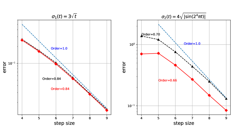
Figure 1. Numerical experiment for SPDE (60): Step sizes versus $L^{2}$ errors

The results of our simulations are shown in Figure 1. We plot the Monte Carlo estimates of the root-mean-squared errors versus the underlying temporal step size, i.e., the number $i$ on the $x$-axis indicates the corresponding simulation is based on the temporal step size $k=2^{-i}$. The figure on the left hand side shows the results for $\sigma=\sigma_{1}=3\sqrt{t}$, while the right hand shows $\sigma_{2}(t)$. In both subfigures, the sets of data points on the black dotted curves with triangle markers show the errors of the classical Galerkin finite element method, while the red-dotted error curves with diamond markers correspond to the simulations of the randomized Galerkin finite element method. In addition, we draw a dashed blue reference line representing a method of order one. The order numbers displayed in the figure correspond to the slope of a best fitting function obtained by linear regression. This might be interpreted as an average order of convergence.

For the case of $\sigma_{1}$, the error curves from both methods are almost overlapping, with the same average order of convergence $0.84$. Since the randomized method is computationally up to twice as expensive as the classical Galerkin finite element method, the latter method is clearly superior in this example. However, as already discussed in Remark 3.8, the results on the error analysis of the classical method currently available in the literature are not able to theoretically explain the same order of convergence for general stochastic evolution equations satisfying Assumptions 3.1 to 3.5.

This is illustrated by the more academic example of $\sigma_{2}$. Here the coefficient function of the noise intensity is chosen in such a way that the classical Galerkin finite element method cannot distinguish between a deterministic PDE without the Wiener noise and the SPDE (60). In fact, for all step sizes $k=2^{i}$ with $i\in\{4,5\}$ the classical method only evaluates $\sigma_{2}$ on its zeros which explains the large errors for those step sizes seen on the right hand side of Figure 1. The randomized method is less severely affected by the highly oscillating coefficient function. For smaller step sizes this advantage then decays.

Table 1. Numerical values of the $L^{2}$-errors and experimental order of convergence (EOC) for the simulations shown in Figure 1.

		$\sigma_{1}(t)=$	$3\sqrt{t}$			$\sigma_{2}(t)=$	$4\sqrt{|\sin(16\pi t)|}$
	classic GFEM		rand. GFEM		classic GFEM		rand. GFEM
$k$	error	EOC	error	EOC	error	EOC	error	EOC
0.0625	0.2696		0.2601		1.3812		0.7034
0.0312	0.1688	0.67	0.1636	0.67	1.2082	0.19	0.7205	-0.03
0.0156	0.1023	0.72	0.0974	0.75	0.7595	0.67	0.4611	0.64
0.0078	0.0553	0.89	0.0531	0.87	0.4398	0.79	0.2699	0.77
0.0039	0.0287	0.95	0.0280	0.93	0.2501	0.81	0.1481	0.87
0.0020	0.0151	0.93	0.0144	0.96	0.1312	0.93	0.0842	0.81

Table 1 contains the numerical values of the error data displayed in Figure 1. In addition, we computed the corresponding experimental orders of convergence defined by

$$\mbox{EOC}=\dfrac{\log(\mbox{error}(2^{-i}))-\log(\mbox{error}(2^{-i+1}))}{\log(2^{-i})-\log(2^{-i+1})}$$

for $i\in\{5,6,7,8,9\}$, where the term $\mbox{error}(2^{-i})$ denotes the error of step size $2^{-i}$.

References

[1]
A. Barth and A. Lang.
Milstein approximation for advection-diffusion equations driven by
multiplicative noncontinuous martingale noises.
Appl. Math. Optim., 66(3):387–413, 2012.
[2]
A. Barth and A. Lang.
and almost sure convergence of a Milstein scheme for
stochastic partial differential equations.
Stochastic Process. Appl., 123(5):1563–1587, 2013.
[3]
A. Barth, A. Lang, and C. Schwab.
Multilevel Monte Carlo method for parabolic stochastic partial
differential equations.
BIT, 53(1):3–27, 2013.
[4]
S. Becker, A. Jentzen, and P. E. Kloeden.
An exponential Wagner–Platen type scheme for SPDEs.
SIAM J. Numer. Anal., 54(4):2389–2426, 2016.
[5]
W.-J. Beyn and R. Kruse.
Two-sided error estimates for the stochastic theta method.
Discrete Contin. Dyn. Syst. Ser. B, 14(2):389–407, 2010.
[6]
D. L. Burkholder.
Explorations in martingale theory and its applications.
In École d’Été de Probabilités de Saint-Flour
XIX—1989, volume 1464 of Lecture Notes in Math., pages 1–66.
Springer, Berlin, 1991.
[7]
G. Da Prato and J. Zabczyk.
Stochastic Equations in Infinite Dimensions, volume 44 of Encyclopedia of Mathematics and its Applications.
Cambridge University Press, Cambridge, 1992.
[8]
E. Di Nezza, G. Palatucci, and E. Valdinoci.
Hitchhiker’s guide to the fractional Sobolev spaces.
Bull. Sci. Math., 136(5):521–573, 2012.
[9]
M. Eisenmann, M. Kovács, R. Kruse, and S. Larsson.
On a randomized backward Euler method for nonlinear evolution
equations with time-irregular coefficients.
ArXiv preprint, arXiv:1709:01018, 2017.
[10]
M. Eisenmann and R. Kruse.
Two quadrature rules for stochastic Itō-integrals with
fractional Sobolev regularity.
ArXiv preprint, arXiv:1712.08152, 2017.
[11]
D. Gilbarg and N. S. Trudinger.
Elliptic partial differential equations of second order.
Classics in Mathematics. Springer-Verlag, Berlin, 2001.
Reprint of the 1998 edition.
[12]
S. Haber.
A modified Monte-Carlo quadrature.
Math. Comp., 20:361–368, 1966.
[13]
S. Haber.
A modified Monte-Carlo quadrature. II.
Math. Comp., 21:388–397, 1967.
[15]
M. Hofmanová, M. Knöller, and K. Schratz.
Stratified exponential integrator for modulated nonlinear
Schrödinger equations.
ArXiv preprint, arXiv:1711.01091, 2017.
[16]
A. Jentzen and P. E. Kloeden.
Taylor Approximations for Stochastic Partial Differential
Equations, volume 83 of CBMS-NSF Regional Conference Series in Applied
Mathematics.
Society for Industrial and Applied Mathematics (SIAM), Philadelphia,
PA, 2011.
[17]
A. Jentzen and M. Röckner.
A Milstein scheme for SPDEs.
Found. Comput. Math., 15(2):313–362, 2015.
[18]
R. Kruse.
Consistency and stability of a Milstein–Galerkin finite element
scheme for semilinear SPDE.
Stoch. Partial Differ. Equ. Anal. Comput., 2(4):471–516, 2014.
[19]
R. Kruse.
Strong and Weak Approximation of Stochastic Evolution
Equations, volume 2093 of Lecture Notes in Mathematics.
Springer, 2014.
[20]
R. Kruse and Y. Wu.
Error analysis of randomized Runge–Kutta methods for differential
equations with time-irregular coefficients.
Comput. Methods Appl. Math., 17(3):479–498, 2017.
[21]
R. Kruse and Y. Wu.
A randomized Milstein method for stochastic differential equations
with non-differentiable drift coefficients.
ArXiv preprint, arXiv:1706.09964, 2017.
[22]
S. Larsson and V. Thomée.
Partial Differential Equations with Numerical Methods,
volume 45 of Texts in Applied Mathematics.
Springer-Verlag, Berlin, 2009.
Paperback reprint of the 2003 edition.
[23]
C. Leonhard and A. Rößler.
An efficient derivative-free Milstein scheme for stochastic partial
differential equations with commutative noise.
ArXiv preprint, arXiv:1509.08427, 2015.
[24]
G. J. Lord, C. E. Powell, and T. Shardlow.
An Introduction to Computational Stochastic PDEs.
Cambridge Texts in Applied Mathematics. Cambridge University Press,
New York, 2014.
[25]
G. J. Lord and A. Tambue.
Stochastic exponential integrators for the finite element
discretization of SPDEs for multiplicative and additive noise.
IMA J. Numer. Anal., 33(2):515–543, 2013.
[26]
A. Pazy.
Semigroups of Linear Operators and Applications to Partial
Differential Equations, volume 44 of Applied Mathematical Sciences.
Springer, New York, 1983.
[27]
C. Prévôt and M. Röckner.
A concise course on stochastic partial differential equations,
volume 1905 of Lecture Notes in Mathematics.
Springer, 2007.
[28]
J. Simon.
Sobolev, Besov and Nikolskiĭ fractional spaces: imbeddings
and comparisons for vector valued spaces on an interval.
Ann. Mat. Pura Appl. (4), 157:117–148, 1990.
[29]
M. N. Spijker.
Stability and convergence of finite-difference methods, volume
1968 of Doctoral dissertation, University of Leiden.
Rijksuniversiteit te Leiden, Leiden, 1968.
[30]
M. N. Spijker.
On the structure of error estimates for finite-difference methods.
Numer. Math., 18:73–100, 1971/72.
[31]
F. Stummel.
Approximation methods in analysis.
Matematisk Institut, Aarhus Universitet, Aarhus, 1973.
Lectures delivered during the spring term, 1973, Lecture Notes
Series, No. 35.
[32]
V. Thomée.
Galerkin Finite Element Methods for Parabolic Problems,
volume 25 of Springer Series in Computational Mathematics.
Springer-Verlag, Berlin, second edition, 2006.
[33]
X. Wang.
An exponential integrator scheme for time discretization of nonlinear
stochastic wave equation.
J.Sci. Comput., 64(1):234–263, 2015.
[34]
X. Wang.
Strong convergence rates of the linear implicit Euler method for
the finite element discretization of SPDEs with additive noise.
IMA J. Numer. Anal., 37(2):965–984, 2017.