A classification of 3+1D bosonic topological orders (II):
the case when some pointlike excitations are fermions

Abstract

In this paper, we classify EF topological orders for 3+1D bosonic systems where some emergent pointlike excitations are fermions. (1) We argue that all 3+1D bosonic topological orders have gappable boundary. (2) All the pointlike excitations in EF topological orders are described by the representations of $G_{f}=Z_{2}^{f}\leftthreetimes_{e_{2}}G_{b}$ – a $Z_{2}^{f}$ central extension of a finite group $G_{b}$ characterized by $e_{2}\in H^{2}(G_{b},Z_{2})$. (3) We find that the EF topological orders are classified by 2+1D anomalous topological orders $\mathcal{A}_{b}^{3}$ on their unique canonical boundary. Here $\mathcal{A}_{b}^{3}$ is a unitary fusion 2-category with simple objects labeled by $\hat{G}_{b}=Z_{2}^{m}\leftthreetimes G_{b}$. $\mathcal{A}_{b}^{3}$ also has one invertible fermionic 1-morphism for each object as well as quantum-dimension-$\sqrt{2}$ 1-morphisms that connect two objects $g$ and $gm$, where $g\in\hat{G}_{b}$ and $m$ is the generator of $Z_{2}^{m}$. (4) When $\hat{G}_{b}$ is the trivial $Z_{2}^{m}$ extension, the EF topological orders are called EF1 topological orders, which is classified by simple data $(G_{b},e_{2},n_{3},\nu_{4})$, where $n_{3}\in H^{3}(G_{b},Z_{2})$, and $\nu_{4}$ is a 4-cochain in $C^{4}(G_{b},U(1))$ satisfying $\text{d}\nu_{4}=(-)^{n_{3}\smile n_{3}+e_{2}\smile n_{3}}$. (5) When $\hat{G}_{b}$ is a non-trivial $Z_{2}^{m}$ extension, the EF topological orders are called EF2 topological orders, where some intersections of three stringlike excitations must carry Majorana zero modes. (6) Every EF2 topological order with $G_{f}=Z_{2}^{f}\leftthreetimes G_{b}$ can be associated with a EF1 topological order with $G_{f}=Z_{2}^{f}\leftthreetimes\hat{G}_{b}$, which may leads to an understanding of EF2 topological orders in terms of simpler EF1 topological orders. (7) We find that all EF topological orders correspond to gauged 3+1D fermionic symmetry protected topological (SPT) orders with a finite unitary symmetry group. Our results can also be viewed as a classification of the corresponding 3+1D fermionic SPT orders. (8) We further propose that the general classification of 3+1D topological orders with finite unitary symmetries for bosonic and fermionic systems can be obtained by gauging or partially gauging the finite symmetry group of 3+1D SPT phases of bosonic and fermionic systems.

I Introduction

In LABEL:LW170404221, we classified the so called all-boson (AB) 3+1D topological orders – the 3+1D topological orders whose emergent pointlike excitations are all bosonic. We found that All 3+1D AB topological orders are classified by pointed unitary fusion 2-categories with trivial 1-morphisms, which are one-to-one labeled by a pair $(G,\omega_{4})$ up to group automorphisms, where $G$ is a finite group and $\omega_{4}$ its group 4-cohomology class: $\omega_{4}\in H^{4}(G;\mathbb{R}/\mathbb{Z})$.

In this paper, we classify 3+1D topological orders with emergent fermionic pointlike excitations, which will be called EF topological orders. The results in LABEL:LW170404221 and in this paper classify all 3+1D topological orders in bosonic systems. This result in turn leads to a classification of 3+1D topological orders with finite unitary symmetry for bosonic and fermionic systems. In addition, we argue that all 3+1D bosonic topological orders always have gappable boundary.

The pointlike excitations and the stringlike excitations in 3+1D bosonic topological orders can fuse and braid, and their fusion and braiding must form a self-consistent structure. In particular, the self-consistent structure must satisfy
The principle of remote detectability: In an anomaly-free topological order, every topological excitation can be detected by other topological excitations via some remote operations. If every topological excitation can be detected by other topological excitations via some remote operations, then the topological order is anomaly-free.
Here “anomaly-free” means realizable by a local bosonic lattice model in the same dimension Wen (2013). The remote detectability condition is also the anomaly-free condition.

Since the remote detection is done by braiding, the self consistency of fusion and braiding, plus the remote detectability can totally fix the structure of pointlike and stringlike excitations. Those structures in turn classify the 3+1D EF topological orders.

II Summary of results

II.1 Emergence of a group $G_{f}$

In particular, we show that the pointlike excitations are described by a symmetric fusion category $\mathrm{s}\mathcal{R}\mathrm{ep}(G_{f})$. In other words, each type of pointlike excitations correspond to an irreducible representation of a finite group $G_{f}$. The quantum dimension of the excitations is given by the dimension of the representation. $G_{f}$ is a $Z_{2}^{f}$ central extension of $G_{b}$:

$$1\to Z_{2}^{f}\to G_{f}\stackrel{{\scriptstyle\pi^{f}}}{{\to}}G_{b}\to 1.$$ (1)

The excitation is fermionic if $Z_{2}^{f}$ is represented non-trivially in the representation. Otherwise, the excitation is bosonic.

II.2 Unique canonical gapped boundary described by a unitary fusion 2-category

Following a similar approach proposed in LABEL:LW170404221, in this paper, we show that all EF topological orders have a unique canonical gapped boundary, which is described by a unitary fusion 2-category $\mathcal{A}_{b}^{3}$. Let us describe such fusion 2-categories in details. The simple objects of fusion 2-category, corresponding to the boundary strings, are labeled by $\hat{G}_{b}$. Here $\hat{G}_{b}$ is an extension of $G_{b}$ by $Z_{2}^{m}$:

$$1\to Z_{2}^{m}\to\hat{G}_{b}\stackrel{{\scriptstyle\pi^{m}}}{{\to}}G_{b}\to 1.$$ (2)

The fusion of those boundary strings (the objects) is described by the group multiplication of $\hat{G}_{b}$.

In the fusion 2-category, there is a 1-morphism of unit quantum dimension that connects each simple object $g$ to itself. Such a 1-morphism correspond to a pointlike topological excitation living on the string $g$. But this pointlike excitation is not confined to certain strings; they can move freely on the boundary and braid among themselves. The statistics of this pointlike excitation (the 1-morphism) is fermionic. So the canonical boundary of a EF topological order also contains a fermion in addition to the boundary strings.

There is also a 1-morphism of quantum dimension $\sqrt{2}$ that connects object $g$ to object $gm$ where $m$ is the generator of $Z_{2}^{m}$. Physically, it means that the domain wall between string $g$ and string $gm$ carries a fractional degrees of freedom of dimension $\sqrt{2}$ (i.e. like one half of a qubit). There is no other 1-morphisms.

In this paper, we show that each EF topological order corresponds to one such fusion 2-category. LABEL:ZLW shows that for each of such fusion 2-categories, one can construct a bosonic model to realize a EF topological order who has a boundary described by the fusion 2-category. Thus, the classification of such unitary fusion 2-categories corresponds to a classification of 3+1D EF topological orders.

We note that the boundary fermion can form a $p$-wave topological superconducting chain,Kitaev (2001) which is called a Majorana chain. In fact, two boundary strings labeled by $g$ and $gm$ differ by attaching such a Majorana chain. The 1-morphism of quantum dimension $\sqrt{2}$ at the domain wall between the strings $g$ and $gm$ is nothing but the Majorana zero mode at the end of the Majorana chain.

Figure 1: A string configuration in the bulk described by a triple $(\chi_{g^{f}_{1}},\chi_{g^{f}_{2}},[g_{3}^{f}])$, where $\chi_{g^{f}}$ is a conjugacy class in $G_{f}$ containing $g^{f}\in G_{f}$ and the triple satisfy $g_{1}^{f}g_{2}^{f}=g_{3}^{f}$.

II.3 Emergence of Majorana zero modes

The above classification of EF topological orders allows us to divide those EF topological orders into EF1 topological orders when $\hat{G}_{b}=Z_{2}^{m}\times G_{b}$, and EF2 topological orders when $\hat{G}_{b}$ is a non-trivial $Z_{2}^{m}$ extension of $G_{b}$, described by a group 2-cocycle $\rho_{2}(g_{b},h_{b})\in H^{2}(G_{b},Z_{2}^{m})$. In the following, we will describe how to directly measure the group 2-cocycle $\rho_{2}$ via the Majorana zero modes carried by the intersections of three strings.

Consider a fixed set of strings labeled by $\chi_{g^{f}}$ where $\chi_{g^{f}}$ is a conjugacy class in $G_{f}$ that containing $g^{f}\in G_{f}$. Three strings $\chi_{g^{f}_{1}}$, $\chi_{g^{f}_{2}}$, and $\chi_{g^{f}_{3}}$ can annihilate if $g_{1}^{f}g_{2}^{f}=g_{3}^{f}$. If the triple string intersection has a Majorana zero mode, we assign $\rho^{f}_{2}(g_{1}^{f},g_{2}^{f})=-1$. If the triple string intersection has no Majorana zero mode, we assign $\rho^{f}_{2}(g_{1}^{f},g_{2}^{f})=1$. (When $G_{f}$ is Abelian, the apearance of Majorana zero modes can be determined by the 2-fold topological degeneracy for the configuration Fig. 1.) $\rho^{f}_{2}(g_{1}^{f},g_{2}^{f})$ only depends on the conjugacy classes of $g_{1}^{f}$, $g_{2}^{f}$, and $g_{3}^{f}$. Thus $\rho^{f}_{2}$ satisfies

$$\rho^{f}_{2}(g_{1}^{f},g_{2}^{f})=\rho^{f}_{2}(h_{1}g_{1}^{f}h_{1}^{-1},h_{2}g_{2}^{f}h_{2}^{-1}),\ \ \ \ h_{1},h_{2}\in G_{f}.$$ (3)

It turns out that $\rho^{f}_{2}(g_{1}^{f},g_{2}^{f})$ is actually a function on $G_{b}$, i.e. it has a form

$$\rho^{f}_{2}(g_{1}^{f},g_{2}^{f})=\tilde{\rho}_{2}[\pi^{f}(g_{1}^{f}),\pi^{f}(g_{2}^{f})].$$ (4)

$\tilde{\rho}_{2}$ in the above is cohomologically equivalent to $\rho_{2}$ that describes the extension $\hat{G}_{b}$; in other words, we measured $\rho_{2}$ up to coboundaries. If the measured $\rho_{2}$ is trivial in $H^{2}(G_{b},Z_{2}^{m})$, the corresponding bulk topological order is a EF1 topological order. If the measured $\rho_{2}$ is a non-trivial cocycle, we get a EF2 topological order.

II.4 Classification of EF1 topological order by a class of pointed unitary fusion 2-category

For an EF1 topological order, the unitary fusion 2-category that describe its canonical boundary can be simplified, since we can treat the Majorana chain as a trivial string when $\hat{G}_{b}=Z_{2}^{m}\times G_{b}$. The simplified unitary fusion 2-category $\bar{\mathcal{A}}_{b}^{3}$ has simple objects labeled by $G_{b}$ and an 1-morphism of unit quantum dimension that connects each simple object to itself. There is no other morphisms. We studied this case thoroughly, and showed that $\bar{\mathcal{A}}_{b}^{3}$ are classified by data $(G_{b},e_{2},n_{3},\nu_{4})$, where $G_{b}=G_{f}/Z_{2}^{f}$, $e_{2}\in H^{2}(G_{b},\mathbb{Z}_{2})$ the 2-cocycle determining the extension $Z_{2}^{f}\to G_{f}\to G_{b}$, $n_{3}\in H^{3}(G_{b},\mathbb{Z}_{2})$, and $\nu_{4}$ is a 4-cochain in $C^{4}(G_{b},U(1))$ satisfying

$$\hskip 1.0pt\mathrm{d}\nu_{4}=(-)^{n_{3}\underset{{\scriptscriptstyle 1}}{\smile}n_{3}+e_{2}\underset{{\scriptscriptstyle}}{\smile}n_{3}}.$$ (5)

The above data $(G_{b},e_{2},n_{3},\nu_{4})$ classify the EF1 topological orders. This result is closely related to a partial classification of fermionic symmetry-protected topological (SPT) phases Gu and Wen (2014), where a similar twisted cocycle condition eqn. (5) was first obtained (without the $e_{2}\underset{{\scriptscriptstyle}}{\smile}n_{3}$ term).

Given a unitary fusion 2-categories $\mathcal{A}_{b}^{3}$ in Section II.2, we can obtain a pointed unitary fusion 2-categories $\bar{\mathcal{A}}_{b}^{3}$ by ignoring the quantum-dimension-$\sqrt{2}$ 1-morphisms. Thus there is a map from the unitary fusion 2-categories $\mathcal{A}_{b}^{3}$ to the pointed unitary fusion 2-categories $\bar{\mathcal{A}}_{b}^{3}$. In other words, there is a map from EF topological orders to EF1 topological orders. This relation allows us to construct a generic EF topological order from a EF1 topological order.

II.5 A general classification of 3+1D topological orders with finite unitary symmetry for bosonic and fermionic systems

With the above classification results, we further propose that the general classification of 3+1D topological orders with symmetries can be obtained by gauging 3+1D SPT phases. Partially gauging a SPT phase leads to a phase with both topological order and symmetry, namely a symmetry-enriched topological (SET) phase, while fully gauging the symmetry leads to an intrinsic topological order. The phases in the same gauging sequence share the same classification data, as the starting SPT phase and the ending topological order coincide in their classification.

II.6 The line of arguments

The key result of this paper, the classification of 3+1D EF topological orders is obtained via the following line of arguments. We first show that condensing all the bosonic pointlike excitation in a 3+1D EF topological order always give rise to a unique $Z_{2}^{f}$ topological order (see Section III). We then show that there is a gapped domain wall between the EF and the $Z_{2}^{f}$ topological orders (see Section V), and there is a gapped boundary for the EF topological order (see Section VI). This allows us to show that all 3+1D EF topological orders have gapped boundary. The domain wall and the boundary are described by unitary fusion 2-categories. This leads to a classification of 3+1D EF topological orders in terms of a subclass of unitary fusion 2-categories.

III Condensing all the bosonic pointlike excitations to obtain a $Z_{2}^{f}$ topological order

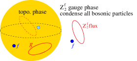
Figure 2: Condensing all bosonic pointlike excitations in a 3+1D EF topological order $\mathcal{C}^{4}_{EF}$ gives rise to 3+1D $Z_{2}^{f}$ topological order $\mathcal{C}^{4}_{Z_{2}^{f}}$. $\mathcal{C}^{4}_{EF}$ contain a fermionic pointlike excitation $f$, and a stringlike excitation, $Z_{2}^{f}$-flux, which behave like the $\pi$-flux line for the fermion $f$. The domain wall $\mathcal{A}_{w}^{3}$ between $\mathcal{C}^{4}_{EF}$ and $\mathcal{C}^{4}_{Z_{2}^{f}}$ contain strings labeled by elements $g\in G_{f}$ and only one fermionic particle $f$. The strings and the fermion have quantum dimension 1.

Some pointlike excitations in a 3+1D EF topological order are bosons and the others are fermions. In this section, we show that, by condensing all the bosonic pointlike excitations, we will always ends up with a simple $Z_{2}^{f}$ topological order – a topological order described by 3+1D $Z_{2}$ gauge theory, but with a fermionic $Z_{2}$ charge Levin and Wen (2005) (see Fig. 2). In the next a few subsections, we will introduce related concepts and pictures that allow us to obtain such a result.

III.1 Pointlike excitations and group structure in 3+1D EF topological orders

The pointlike excitations in 3+1D EF topological orders are described by SFC. According to Tannaka duality (see Appendiex A), the SFC give rise to a group $G_{f}$ such that the pointlike excitations are labeled by the irreducible representations of $G_{f}$. In addition, $G_{f}$ contains a $Z_{2}$ central subgroup, denoted by $Z_{2}^{f}=\{\mathbf{1},z\}$. In each irreducible representations of $G_{f}$, $z$ is either represented by $I$ or $-I$ (where $I$ is an identity matrix). If $z=I$, the corresponding pointlike excitation is a boson. We note that all the bosonic pointlike excitations are described by irreducible representations of $G_{b}$, $\mathcal{R}\mathrm{ep}(G_{b})$, where $G_{b}=G_{f}/Z_{2}^{f}$. If $z=-I$, the corresponding pointlike excitation is a fermion. We denote such SFC by $\mathrm{s}\mathcal{R}\mathrm{ep}(G_{f})$. We see that each 3+1D EF topological order correspond to a pair of groups $(G_{f},Z_{2}^{f})$ where $Z_{2}^{f}$ is the $Z_{2}$ central subgroup of $G_{f}$.

III.2 Stringlike excitations in 3+1D EF topological orders

The pointlike excitations have trivial mutual statistics among them. One cannot use the pointlike excitations to detect other pointlike excitations by remote operations. Thus, based on the principle of remote detectability, there must stringlike excitations in 3+1D EF topological orders, so that every pointlike excitation can be detected by some stringlike excitations via remote braiding. Similarly, every stringlike excitation can be detected by some pointlike and/or stringlike excitations via remote braiding. We see that the properties of stringlike excitations are determined by the pointlike topological excitations (i.e. $\mathrm{s}\mathcal{R}\mathrm{ep}(G)$) to a certain degree.

Let us discuss some basic properties of stringlike excitations. First, similar to the particle case, a stringlike excitation $s_{i}$ can be defined via a trap Hamiltonian $\Delta H_{\text{str}}(s_{i})$ which is non-zero along a loop. The ground state subspace of total Hamiltonian $H_{0}+\sum_{i}\Delta H_{\text{str}}(s_{i})$ define the fusion space of strings $s_{i}$ (and particles $p_{i}$ if we also have particle traps $\Delta H(p_{i})$): ${\cal V}(M,p_{1},p_{2},\cdots,s_{1},s_{2},\cdots)$. We note that such a definition relies on an assumption that all the on-string excitations are gapped. We argued that this is always the case Lan et al. (2017a):
A stringlike excitation $s_{i}$ is called simple if its fusion space cannot be split by any non-local perturbations along the string (i.e. the ground state degeneracy cannot be split by any non-local perturbations of $\Delta H_{\text{str}}(s_{i})$.)
We stress that here we allow non-local perturbations which are non-zero only along the string. The motivation to use non-local perturbations is that we want separate out the degeneracy that is “distributed” between strings and particles. The degeneracy caused by a single string is regarded as “accidental” degeneracy.

For example, in a 3+1D $Z_{2}$-gauge theory, the $Z_{2}$-gauge-charge has a mod 2 conservation. Those $Z_{2}$-charges can form a many-body state along a large loop, that spontaneously break the mod 2 conservation which leads to a 2-fold degeneracy. We do not want to regard such a string as a non-trivial simple string. One way to remove such kinds of string as a non-trivial simple string is to require the stability against non-local perturbations along a simple string. Mathematically, if we allow non-local perturbations as morphisms, the above string from $Z_{2}$-charge condensation become a direct sum of two trivial strings.

The fusion of simple strings may give us non-simple strings which can be written as a direct sum of simple strings

$$s_{i}\otimes s_{j}=\bigoplus_{k}M^{ij}_{k}s_{k}.$$ (6)

Using $M^{ij}_{k}$ we can also compute the dimension of the fusion space when we fuse $n$ unlinked loops $s_{i}$ in the large $n$ limit, which is of order $\sim d_{s_{i}}^{n}$. This allows us define the quantum dimension of the $s_{i}$ string.

Strings (when they are simple contractable loops $S^{1}$) can also shrink to a point and become pointlike excitations:

$$s_{i}\to\bigoplus_{j}L^{i}_{j}p_{j}.$$ (7)

If the shrinking of a string does not contain $\mathbf{1}$, then we say that the string is not pure. Such a non-pure string can be viewed as a bound state of pure string with some topological pointlike excitations.

In fact, not only strings have shrinking operation, particles also have shrinking operation. We note that a zero-dimension sphere $S^{0}$ is two points, which may correspond to a pair of particles $(p_{1},p_{2})$. Thus in various dimensions $n$, we may have excitations described by $S^{d}$. For $d=0,1,2,\cdots$, they correspond to a pair of particles $(p_{1},p_{2})$, a loop excitation $s$, a spherical membrane excitation $m$, etc . Those excitations are pure if their shrinking contains $\mathbf{1}$. For example an $S^{0}$ excitation $(p_{1},p_{2})$ is pure iff $p_{2}$ is the anti particle of $p_{1}$.

There is a well known result that $p$ is simple iff the shrinking of $p$ and $\bar{p}$ (i.e. the fusion of $p$ and $\bar{p}$) contains only a single trivial particle $\mathbf{1}$. In this case, we also say that the corresponding pure $S^{0}$ excitation $(p,\bar{p})$ is simple. Similarly, we believe that
A string $s$ is not simple if the shrinking of $s$ contains more than one trivial particles $\mathbf{1}$: $s\to n\mathbf{1}\oplus\cdots$, $n>1$.

In this paper, we will refer to the number of simple stringlike excitations as the number of types. We will refer to the number of pure simple stringlike excitations as number of pure types. A string $s$ with quantum dimension $1$ is always simple. Such a string is invertible or pointed, i.e. there exists another string $s^{\prime}$ such that

$$s\otimes s^{\prime}=s^{\prime}\otimes s=\mathbf{1}.$$ (8)

For a more detailed discussion about stringlike excitations and their related membrane operators, see LABEL:LW170404221.

III.3 Dimension reduction of generic topological orders

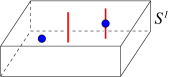
Figure 3: (Color online) The dimension reduction of 3D space $M^{2}\times S^{1}$ to 2D space $M^{2}$. The top and the bottom surfaces are identified and the vertical direction is the compactified $S^{1}$ direction. A 3D pointlike excitation (the blue dot) becomes an anyon particle in 2D. A 3D stringlike excitation wrapping around $S^{1}$ (the red line) also becomes an anyon particle in 2D.

We can reduce a $3+1$D topological order $\mathcal{C}^{4}$ on space-time $M^{3}\times S^{1}$ to $2+1$D topological orders on space-time $M^{3}$ by making the circle $S^{1}$ small (see Fig. 3) Moradi and Wen (2015); Wang and Wen (2015). In this limit, the $3+1$D topological order $\mathcal{C}^{d+1}$ can be viewed as several $2+1$D topological orders $\mathcal{C}^{3}_{i}$, $i=1,2,\cdots,N^{\text{sec}}_{1}$ which happen to have degenerate ground state energy. We denote such a dimensional reduction process by

$$\mathcal{C}^{4}=\bigoplus_{i=1}^{N^{\text{sec}}_{1}}\mathcal{C}^{3}_{i},$$ (9)

where $N^{\text{sec}}_{1}$ is the number of sectors produced by the dimensional reduction.

We note that the different sectors come from the different holonomy of moving pointlike excitations around the $S^{1}$ (see Fig. 3). So the dimension reduction always contain a sector where the holonomy of moving any pointlike excitations around the $S^{1}$ is trivial. Such a sector will be called the untwisted sector.

In the untwisted sector, there are three kinds of anyons. The first kind of anyons correspond to the 3+1D pointlike excitations. The second kind of anyons correspond to the 3+1D pure stringlike excitations wrapping around the compactified $S^{1}$. The third kind of anyons are bound states of the first two kinds (see Fig. 3).

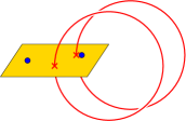
Figure 4: (Color online) The untwisted sector in the dimension reduction can be realized directly on a 2D sub-manifold in 3D space without compactification.

We like to point out that the untwisted sector in the dimension reduction can even be realized directly in 3D space without compactification. Consider a 2D sub-manifold in the 3D space (see Fig. 4), and put the 3D pointlike excitations on the 2D sub-manifold. We can have a loop of string across the 2D sub-manifold which can be viewed as an effective pointlike excitation on the 2D sub-manifold. We can also have a bound state of the above two types of effective pointlike excitations on the 2D sub-manifold. Those effective pointlike excitations on the 2D sub-manifold can fuse and braid just like the anyons in 2+1D. The principle of remote detectability requires those effective pointlike excitations to form a unitary modular tensor category (UMTC). When we perform dimension reduction, the above UMTC becomes the untwisted sector of the dimension reduced 2+1D topological order.

Since the dimension reduced 2+1D topological orders must be anomaly-free, they must be described by UMTCs. Since the untwisted sector always contains $\mathrm{s}\mathcal{R}\mathrm{ep}(G_{f})$, we conclude that
The untwisted sector of a dimension reduced 3+1D EF topological order is a modular extension of $\mathrm{s}\mathcal{R}\mathrm{ep}(G_{f})$.

III.4 Untwisted sector of dimension reduction is the 2+1D Drinfeld center

In the following we will show a stronger result, for the dimension reduction of generic 3+1D topological orders. Let the symmetric fusion category formed by the pointlike excitations be $\mathcal{E}$, $\mathcal{E}=\mathcal{R}\mathrm{ep}(G)$ or $\mathcal{E}=\mathrm{s}\mathcal{R}\mathrm{ep}(G_{f})$ for AB or EF cases respectively:
The untwisted sector $\mathcal{C}^{3}_{\text{untw}}$ of dimension reduction of a generic 3+1D topological orders must be the 2+1D topological order described by Drinfeld center of $\mathcal{E}$: $\mathcal{C}^{3}_{\text{untw}}=Z(\mathcal{E})$.
Note that Drinfeld center $Z(\mathcal{E})$ is the minimal modular extension of $\mathcal{E}$.

First, let us recall the definition of Drinfeld center. The Drinfeld center $Z(\mathcal{A})$ of a fusion category $\mathcal{A}$, is a braided fusion category, whose objects are pairs $(A,b_{A,-})$, where $A$ is an object in $\mathcal{A}$, $b_{A,-}$ is a set of isomorphisms $b_{A,X}:A\otimes X\cong X\otimes A,\forall X\in\mathcal{A}$. The isomorphisms $b_{A,X}$ is just the collection of unitary operators that connects the fusion spaces $\cdots\otimes A\otimes X\otimes\cdots$ and $\cdots\otimes X\otimes A\otimes\cdots$ for different backgrounds. They satisfy some self consistent conditions such as the hexagon equation:

$$b_{A,Y}b_{A,X}=b_{A,X\otimes Y},$$ (10)

where we omitted the associativity constraints (or F-matrices) of ${\cal A}$ for simplicity (otherwise there are in addition three F-matrices involved, in total six terms, hence the name hexagon). $b_{A,X}$ is called a half braiding.

Physically, we may view the objects in $\mathcal{A}$ as the pointlike topological excitations living on the boundary of a 2+1D topological order. In general, a boundary excitation trapped by a potential on the boundary cannot be lifted into the bulk. Physically, this mean that as moving the trapping potential into the bulk, the ground state subspace will be joined by some high energy eigenstates to form a new ground state subspace. But we may choose the boundary trapping potential very carefully, so that ground state subspace is formed by accidentally degenerate boundary excitations. In this case, we say that the excitation trapped by the boundary potential is a direct sum of those boundary excitations. Such an excitation correspond to a composite object in the fusion category $\mathcal{A}$. Now the question is that which composite object (or direct sum of boundary excitations) can be lifted into the bulk (i.e. the ground state subspace only rotates by unitary transformation as we move the trapping potential into the bulk)?

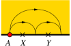
Figure 5: (Color online) If a (composite) boundary excitations can be lifted in to the bulk, its half braiding with other boundary excitations must satisfy some self consistent conditions. The above illustrates the hexagon equation $b_{A,Y}b_{A,X}=b_{A,X\otimes Y}$.

We try to answer this question by exchanging a composite object $A$ in $\mathcal{A}$ with an arbitrary boundary excitation $X$ and study the unitary transformation $b_{A,X}$ induced by such an exchange. If $A$ can be lifted into the bulk, this $b_{A,X}$ can be interpreted as coming from the half braiding (see Fig. 5). There are self consistent conditions from those half braidings. If we find a composite object $A$ whose half braidings satisfy those consistent conditions, we believe that the object $A$ can be lifted into the bulk.

However, there is an additional subtlety: even when we require the ground state subspace only rotates by unitary transformation as we move the trapping potential into the bulk, there are still different ways to move a composite boundary excitation $A$ into the bulk, which lead different pointlike excitations in the bulk. Those different bulk excitations can be distinguished by their different half braiding properties with all the boundary excitations $X$. We assume that all the bulk excitations can be obtained this way. Therefore, the bulk excitations are given by pairs $(A,b_{A,-})$, which correspond to the objects in the Drinfeld center $Z(\mathcal{A})$.

Mathematically, the morphisms of $Z(\mathcal{E})$ between the pairs $(A,b_{A,-}),(B,b_{B,-})$ is a subset of morphisms between $A,B$, such that they commute with the half braidings $b_{A,-},b_{B,-}$. Two pairs $(A,b_{A,-}),(B,b_{B,-})$ are equivalent if there is an isomorphism in $Z(\mathcal{E})$ between them, namely there is an isomorphism, a collection of unitary operators between the fusion spaces $\cdots\otimes A\otimes\cdots,\cdots\otimes B\otimes\cdots$ that commutes with the half braidings $b_{A,-},b_{B,-}$. The fusion and braiding of $(A,b_{A,-})$’s is given by

$$(A,b_{A,-})\otimes(B,b_{B,-}) =(A\otimes B,(b_{A,-}\otimes\operatorname{id}_{B})(\operatorname{id}_{A}\otimes b_{B,-}),$$

$$c_{(A,b_{A,-}),(B,b_{B,-})} =b_{A,B}.$$ (11)

In other words, to half-braid $A\otimes B$ with $X$, one just half-braids $B$ and $A$ successively with $X$, and the braiding between $(A,b_{A,-})$ and $(B,b_{B,-})$ is nothing but the half braiding.

$\mathcal{C}^{3}_{\text{untw}}=Z(\mathcal{E})$ is the consequence that the strings in the untwisted sectors are in fact shrinkable. From the effective theory point of view, we can shrink a string $s$ (including bound states of particles with strings, in particular, pointlike excitations viewed as bound states with the trivial string) to a pointlike excitation $p^{\text{shr}}_{s}$ in $\mathcal{E}$

$$s\to p^{\text{shr}}_{s}=p_{1}\oplus p_{2}\oplus\dots,\quad p_{1},p_{2},\dots\in\mathcal{E}$$ (12)

So if we only consider fusion, the particles $s,\ p$ in the dimension reduced untwisted sector $\mathcal{C}^{3}_{\text{untw}}$ can all be viewed as the particles in $\mathcal{E}$, regardless if they come from the 3D particles or 3D strings. In particular, the particles from the 3+1D strings $s$ can be viewed as composite particles in $\mathcal{E}$ (see eqn. (12)). Next we consider the braidings of them.

In the untwisted sector, the braiding between strings $s,s^{\prime}$, denoted by $c_{s,s^{\prime}}$, requires string $s^{\prime}$ moving through string $s$, which prohibits shrinking string $s$. However, there is no harm to consider the shrinking if we focus on only the initial and end states of the braiding process.

In particular, the braiding between a string $s$ and a particle $p$, induces an isomorphism between the initial and end states where the string $s$ is shrunk (see Fig. 6)

$$c^{\text{shr}}_{s,p}:p^{\text{shr}}_{s}\otimes p\cong p\otimes p^{\text{shr}}_{s}$$ (13)

which is automatically a half-braiding on the particle $p^{\text{shr}}_{s}$. Thus, $(p^{\text{shr}}_{s},c^{\text{shr}}_{s,-})$, by definition, is an object in the Drinfeld center $Z(\mathcal{E})$.

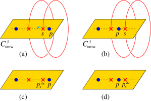
Figure 6: (Color online) From (a) to (b) is the braiding $c_{s,p}$ in the untwisted sector. (c)(d) are obtained from (a)(b) by shrinking strings. Shrinking thus induces a “half-braiding” isomorphism $c^{\text{shr}}_{s,p}$ from (c) to (d).

Shrinking induces a functor

$$\mathcal{C}^{3}_{\text{untw}} \to Z(\mathcal{E})$$

$$s \mapsto(p^{\text{shr}}_{s},c^{\text{shr}}_{s,-})$$ (14)

which is obviously monoidal and braided, i.e. , preserves fusion and braiding. It is also fully faithful, namely bijective on the morphisms. Physically this means that the local operators on both sides are the same. On the left side, morphisms on a string $s$ are operators acting on near (local to) the string $s$; on the right side, morphisms in the Drinfeld center are morphisms on the particle $p^{\text{shr}}_{s}$ which commute with the half braiding $c^{\text{shr}}_{s,-}$. From the shrinking picture, morphisms on $p^{\text{shr}}_{s}$ can be viewed as the operators acting on both near the string $s$ and the interior of the string (namely on a disk $D^{2}$). But in order to commute with $c_{s,p}$ for all $p$, which can be represented by string operators for all $p$ going through the interior of the string $s$ (this includes all possible string operators, because string operators for all particles form a basis), we can take only the operators that act trivially on the interior of the string. Therefore, morphisms on the right side are also operators acting on only near the string. This establishes that the functor is fully faithful, thus a braided monoidal embedding functor; in other words, $\mathcal{C}^{3}_{\text{untw}}$ can be viewed as a full sub-UMTC of $Z(\mathcal{E})$. However, $Z(\mathcal{E})$ is already a minimal modular extension of $\mathcal{E}$, which implies that

$$\mathcal{C}^{3}_{\text{untw}}=Z(\mathcal{E}).$$ (15)

As $Z(\mathcal{E})$ is known well, many properties can be easily extracted. For example, objects in $Z(\mathcal{E})$ have the form $(\chi,\rho)$, where $\chi$ is a conjugacy class, $\rho$ is a representation of the subgroup that centralizes $\chi$. One then concludes
1. A looplike excitation in a 3+1D topological order always has an integer quantum dimension, which is $|\chi|\dim\rho$.
2. Pure strings ($\rho$ trivial) always correspond to conjugacy classes of the group.

In particular, for 3+1D EF topological orders, as the fermion number parity $z$ is in the center of $G_{f}$, its conjugacy class has only one element. We have the following corollary, which is used in later discussions
In all 3+1D EF topological orders, there is an invertible pure $Z_{2}^{f}$ flux loop excitation, corresponding to the conjugacy class of fermion number parity $z$.

III.5 Condensing all the bosonic pointlike excitations

Starting from a 3+1D EF topological order $\mathcal{C}^{4}$, we can condense all the bosonic pointlike excitations described by $\mathcal{R}\mathrm{ep}(G_{b})$, to obtain a new 3+1D EF topological order $\tilde{\mathcal{C}}^{4}$. After $\mathcal{R}\mathrm{ep}(G_{b})$ is condensed, all bosonic pointlike excitations become the trivial pointlike excitation in $\tilde{\mathcal{C}}^{4}$ while all fermionic pointlike excitations become the same fermionic pointlike excitations with quantum dimension 1. In other words, the pointlike excitations in the new topological order $\tilde{\mathcal{C}}^{4}$ are described by $\mathrm{s}\mathcal{R}\mathrm{ep}(Z_{2}^{f})$.

What the stringlike excitations in $\tilde{\mathcal{C}}^{4}$? Although the pointlike excitations in $\tilde{\mathcal{C}}^{4}$ is very simple and can only detect simple strings, the stringlike excitations can braid among themselves and detect each other. Thus $\tilde{\mathcal{C}}^{4}$ might contain complicated stringlike excitations.

However, using the dimension reduction discussed above, the stringlike excitations are determined by the pointlike excitations described by $\mathcal{E}=\mathrm{s}\mathcal{R}\mathrm{ep}(Z_{2}^{f})$. In particular, the untwisted sector of the dimension reduction must be the Drinfeld center $Z(\mathcal{E})=Z[\mathrm{s}\mathcal{R}\mathrm{ep}(Z_{2}^{f})]$, which is nothing but the 2+1D $Z_{2}$-gauge theory. There are only four types of 2+1D anyons: two of them correspond to the 3+1D pointlike excitations in $\mathrm{s}\mathcal{R}\mathrm{ep}(Z_{2}^{f})$ and the other two correspond to the 3+1D stringlike excitations. The fusion rule between the four anyons in the 2+1D $Z_{2}$-gauge theory is described by $Z_{2}\times Z_{2}$ group. This leads to the fusion rule between the loops and the fermion $f$

$$f\otimes f =\mathbf{1},\ \ \ f\otimes s_{1}=s_{2},\ \ \ f\otimes s_{2}=s_{1},\ \ \$$

$$s_{1}\otimes s_{1} =s_{2}\otimes s_{2}=\mathbf{1},\ \ \ s_{1}\otimes s_{2}=f.$$ (16)

The above also implies the shrinking rule for the loops to be

$$s_{1}\to\mathbf{1},\ \ \ \ s_{2}\to f.$$ (17)

We also find that the braiding phases between the fermion $f$ and the two loops $s_{i}$ are given by $-1$, and the braiding phase between two $s_{1}$ or two $s_{2}$’s is $1$. The braiding phase between $s_{1}$ and $s_{2}$ is $-1$. Here the invertible loop $s_{1}$ is the just the $Z_{2}^{f}$ flux loop $z$.

We see that $\tilde{\mathcal{C}}^{4}$ contains only one type of pure simple string $s_{1}$ which shrinks to a single $\mathbf{1}$. The other loop $s_{2}$ is the bound state of $s_{1}$ and the fermion $f$. The loop $s_{1}$ has a trivial two-loop braiding with itself.

How many 3+1D EF topological orders that have the above properties? To answer such a question, we condense the pure string $s_{1}$ in $\tilde{\mathcal{C}}^{4}$ to obtain a topological order $\mathcal{D}^{4}$. Condensing the pure string $s_{1}$ corresponds to condensing the corresponding topological boson in the untwisted sector (which is described by 2+1D $Z_{2}$-gauge theory), which changes the untwisted sector to a trivial phase. So the untwisted sector of dimension reduced $\mathcal{D}^{4}$ is trivial, which implies $\mathcal{D}^{4}$ has no nontrivial particlelike and stringlike excitations.

We can also obtain such a result by noticing that, in $\mathcal{D}^{4}$, the fermions and $s_{2}$ are confined (due to the nontrivial braiding with $s_{1}$) and $s_{1}$ become the ground state (i.e. condensed). Thus $\mathcal{D}^{4}$ has no nontrivial bulk excitations, and must be an invertible topological order. But in 3+1D, all invertible topological orders are trivial Kapustin (2014); Kong and Wen (2014); Freed (2014). Thus $\mathcal{D}^{4}$ is a trivial phase. This means that we can create a boundary of $\tilde{\mathcal{C}}^{4}$ by condensing $s_{1}$ strings. Such a boundary contains only one fermionic particle $f$ with a $Z_{2}$ fusion rule

$$f\otimes f=\mathbf{1}.$$ (18)

So the boundary is described by a so called unitary braided fusion 2-category that has no non-trivial objects and has only one non-trivial 1-morphism that corresponds to a fermion with a $Z_{2}$ fusion. It is nothing but the SFC $\mathrm{s}\mathcal{R}\mathrm{ep}(Z_{2}^{f})$, trivially promoted to a 2-category. Using the principle that boundary uniquely determines the bulk Kong and Wen (2014); Kong et al. (2017), we conclude that all the $\tilde{\mathcal{C}}^{4}$’s that satisfy the above properties are actually the same topological order, which is called $Z_{2}^{f}$ topological order $\mathcal{C}_{Z_{2}^{f}}^{4}$:
Condensing all the bosonic pointlike excitations in $\mathcal{R}\mathrm{ep}(G_{b})$ produces an unique 3+1D topological order $\mathcal{C}_{Z_{2}^{f}}^{4}$.
The topological order $\mathcal{C}_{Z_{2}^{f}}^{4}$ was constructed on a cubic lattice Levin and Wen (2003). It was also called twisted $Z_{2}$ gauge theory where the $Z_{2}$ charge is fermionic, and was realized by 3+1D Levin-Wen string-net model Levin and Wen (2005). $\mathcal{C}_{Z_{2}^{f}}^{4}$ can also be realized by Walker-Wang model von Keyserlingk et al. (2013) or by a 2-cocycle lattice theory Wen (2017). In this paper, we will refer to $\mathcal{C}_{Z_{2}^{f}}^{4}$ as the $Z_{2}^{f}$-topological order.

IV All 3+1D bosonic topological orders have gappable boundary

It is well known that 2+1D topological orders with a non-zero chiral central charge $c$ cannot have gapped boundary. This can be understood from the induced gravitational Chern-Simons term in the effective action for such kind of topological orders. Since there is no gravitational Chern-Simons term in 3+1D. This might suggest that all 3+1D bosonic topological orders have gappable boundary. However, such a reasoning is not correct. In fact, there are 2+1D topological orders with a zero chiral central charge (i.e. with no gravitational Chern-Simons term) that cannot have gapped boundary.Levin (2013)

For a 2+1D topological order described by a unitary modular tensor category (UMTC) $\mathcal{C}^{3}$, if $\mathcal{C}^{3}$ has a condensable algebra, then we can condense the bosons in the condensable algebra to obtain another 2+1D topological order described by a different UMTC $\mathcal{D}^{3}$. Now we like to ask is there a gapped domain wall between the two topological orders $\mathcal{C}^{3}$ and $\mathcal{D}^{3}$? In fact, we can show that there exist a 1+1D anomalous topological order (described by unitary fusion category $\mathcal{A}_{w}^{2}$), such that the Drinfeld center of ${\cal A}^{2}$ is $\mathcal{C}^{3}\boxtimes\bar{\mathcal{D}}^{3}$. Here $\mathcal{C}^{3}\boxtimes\bar{\mathcal{D}}^{3}$ is the 2+1D topological order formed by stacking two topological orders, $\mathcal{C}^{3}$ and $\bar{\mathcal{D}}^{3}$, where $\bar{\mathcal{D}}^{3}$ is the time reversal conjugate of $\mathcal{D}^{3}$. This means that it is consistent to view ${\cal A}^{2}$ as the domain wall between $\mathcal{C}^{3}$ and $\mathcal{D}^{3}$. Then we conjecture that there exist a gapped domain wall between $\mathcal{C}^{3}$ and $\mathcal{D}^{3}$ that is described by $\mathcal{A}_{w}^{2}$.

In the last section, we have seen that condensing all the bosonic excitations described by $\mathcal{R}\mathrm{ep}(G_{b})$ in a 3+1D EF topological order $\mathcal{C}_{EF}^{4}$ give us an unique 3+1D topological order $\mathcal{C}_{Z_{2}^{f}}^{4}$. This result can also be obtained by noticing that the condensation of $\mathcal{R}\mathrm{ep}(G_{b})$ is described by a condensable algebra Kong (2014), and there is only one condensable algebra if we want to condense all $\mathcal{R}\mathrm{ep}(G_{b})$. So there is only one way to condense all $\mathcal{R}\mathrm{ep}(G_{b})$ which produce an unique state $\mathcal{C}_{Z_{2}^{f}}^{4}$.

Such an unique condensation also produces an unique pointed fusion 2-category $\mathcal{A}^{3}_{w}$, such that the generalized Drinfield center of $\mathcal{A}^{3}_{w}$ is $\mathcal{C}_{EF}^{4}\boxtimes\bar{\mathcal{C}}_{Z_{2}^{f}}^{4}$. Thus it is consistent to view $\mathcal{A}^{3}_{w}$ as the canonical domain wall between $\mathcal{C}_{EF}^{4}$ and $\mathcal{C}_{Z_{2}^{f}}^{4}$. This motivate us to conjecture that there exist a gapped domain wall between two 3+1D EF topological orders $\mathcal{C}_{EF}^{4}$ and $\mathcal{C}_{Z_{2}^{f}}^{4}$.

There is a physical argument to support the above conjecture. The particles in the condensable algebra are all bosons which form a SFC $\mathcal{R}\mathrm{ep}(G_{b})$. Those bosons have a emergent symmetry described by $G_{b}$. Since the number of the particle types in the condensable algebra is finite, that requires the number of the irreducible representations of the emergent symmetry group is finite. Thus the emergent symmetry group $G_{b}$ is finite. Those bosons only have short range interaction between them. So the boson condensed phase of those bosons are gapped, with possible ground state degeneracy from the spontaneous breaking of the emergent symmetry $G_{b}$. However since the symmetry is emergent, the symmetry is only approximate in the boson condensed phase. The symmetry breaking term is of an order $\hskip 1.0pt\mathrm{e}^{-l/\xi}$ where $l$ is the mean boson separation in the boson condensed phase and $\xi$ is the correlation length of local operators in the topological order. Since $l$ is finite, the ground state degeneracy is split by a finite amount of order $\hskip 1.0pt\mathrm{e}^{-l/\xi}$. Thus there is no ground state degeneracy in the boson condensed phase. This boson condensed phase corresponds to the $\mathcal{C}_{Z_{2}^{f}}^{4}$ topological order.

The boson condensed state with a small symmetry breaking perturbation is a very simple state in physics which is well studied. Such a state always allows gapped boundary. Therefore, the domain wall between two 3+1D EF topological orders $\mathcal{C}_{EF}^{4}$ and $\mathcal{C}_{Z_{2}^{f}}^{4}$ can always be gapped. In the last section, we showed that $\mathcal{C}_{Z_{2}^{f}}^{4}$ topological order can have a gapped boundary. This allows us to argue that all 3+1D EF topological orders have gappable boundary.

Using a similar argument, we can argue that all 3+1D AB topological orders have gappable boundary. In fact, the argument is much simpler in this case. Hence
all 3+1D bosonic topological orders have gappable boundary.

V Unique canonical domain walls between 3+1D EF topological orders and $Z_{2}^{f}$-topological order $\mathcal{C}_{Z_{2}^{f}}^{4}$

In this section, we describe the properties of the fusion 2-category $\mathcal{A}^{3}_{w}$ and show that those properties are consistent of viewing $\mathcal{A}^{3}_{w}$ as a domain wall between $\mathcal{C}^{4}_{EF}$ and $\mathcal{C}_{Z_{2}^{f}}^{4}$.

V.1 All simple boundary strings and boundary particles have quantum dimension 1

After condensing all bosonic particles $\mathcal{R}\mathrm{ep}(G_{b})$, the only non-trivial particle on the canonical domain wall is the fermion $f$ with quantum dimension 1. Such a fermion can be lifted into one side of the domain wall with the $Z_{2}^{f}$ topological order $\mathcal{C}_{Z_{2}^{f}}^{4}$. On the other side of the domain wall with 3+1D EF topological order $\mathcal{C}^{4}$, if we bring the fermions in $\mathrm{s}\mathcal{R}\mathrm{ep}(G_{f})$ to the boundary, it will become a direct sum (i.e. accidental degenerate copies) of several $f$’s.

What are the stringlike excitations on the domain wall? On the $\mathcal{C}_{Z_{2}^{f}}^{4}$ side of domain wall, there is only one type of pure simple stringlike excitations – the $Z_{2}^{f}$ flux loop with quantum dimension 1. Bring such string to the domain wall will give us a $Z_{2}^{f}$ flux loop on the wall. We can also bring strings in $\mathcal{C}^{4}$ to the domain wall. In general, a string in $\mathcal{C}^{4}$ will become a direct sum of simple boundary strings.

Let us focus on the simple loop excitations on the canonical domain wall. A loop excitation shrunk to a point may become a direct sum of pointlike excitations (see eqn. (7))

$$s\to n\mathbf{1}\oplus mf$$ (19)

where $\mathbf{1}$ and $f$ are the trivial and fermionic pointlike excitations respectively. When $n=0$, the string is not pure. Another possibility is that $n>1$. In this case the string is not simple. When $m>1$ the string is also not simple, since when $s$ fuses with an invertible fermion, its shrinking rule will become

$$s\otimes f\to m\mathbf{1}\oplus nf,$$ (20)

which is not simple. Therefore, simple loop excitations on the domain wall have three possible shrinking rules

$$s_{b}\to\mathbf{1},\ \ \ s_{f}\to f,\ \ \ s_{K}\to\mathbf{1}\oplus f.$$ (21)

In the following we would like to show, by contradiction, that a simple string like $s_{K}$ with quantum dimension $2$ can not exist on the domain wall.

First, the invertible $Z_{2}^{f}$ flux loop $z$, exists in both sides, $\mathcal{C}^{4}$ and $\mathcal{C}_{Z_{2}^{f}}^{4}$, of the domain wall. We are able to braid $z$ around the domain wall excitations. As $z$ is invertible, such braiding leads to only a $U(1)$ phases factor, denoted by $\theta(z,-)$. In particular, $\theta(z,f)=-1$, which is the defining property of $Z_{2}^{f}$ flux.

Second, fusing a fermion $f$ to a string $s_{K}$ which shrinks to $1\oplus f$, will not change the string, namely $s_{K}\otimes f=s_{K}$. Thus,

$$\theta(z,s_{K})=\theta(z,s_{K}\otimes f)=\theta(z,s_{K})\theta(z,f)=-\theta(z,s_{K}),$$ (22)

which is contradictory. Physically, we can use the braiding of $z$ to detect the fermion number parity on the domain wall, which implies that excitations without fixed fermion number parity, such as $s_{k}\to 1\oplus f$, can not be stable on the domain wall. Therefore, there is no simple domain-wall string with quantum dimension $2$.

Thus, a simple loop on the boundary shrinks to a unique particle, $\mathbf{1}$ or $f$, with quantum dimension 1. A simple pure loop on the boundary always shrinks to a single $\mathbf{1}$. This is an essential property in the following discussions:
All simple pure loops on the domain wall have a quantum dimension $d=1$, and their fusion is grouplike.
As the non-pure simple loops are all bound states of $f$ with pure simple loops, we will consider only the simple pure loops. For the moment, we denote the group formed by the simple pure loops on the domain wall under fusion (see Fig. 9), by $H$.

V.2 Fusion of domain-wall strings recover the group

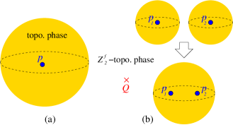
Figure 7: (Color online) (a) The fusion space $F(p)$ for a 3-disk $D^{3}$ containing only one particle $p$. (b) Merging two 3-disks to one 3-disk induces an isomorphism $F(p_{1})\otimes_{\mathbb{C}}F(p_{2})\cong F(p_{1}\otimes p_{2})$.

The argument in this subsection is almost parallel to those in the AB case described in LABEL:LW170404221. There are only a few modifications to address the fermionic nature. But to be self-contained we include a full argument here.

To apply the Tannaka duality (see Appendiex A), we need a physical realization of the super fiber functor. Consider a simple topology for the domain wall: put the 3+1D topological order $\mathcal{C}^{4}$ in a 3-disk $D^{3}$, the domain wall on $\partial D^{3}=S^{2}$, and outside is the condensed phase $\mathcal{C}_{Z_{2}^{f}}^{4}$. When there is only a particle $p$ in the 3-disk, a background particle $Q=\mathbf{1}\oplus f$ in the condensed phase $\mathcal{C}_{Z_{2}^{f}}^{4}$, with no string and no other particles, we associate the corresponding fusion space to the particle $p$, and denote this fusion space by $F(p)$ (see Fig. 7). Viewed from very far away, a 3-disk containing a particle $p$ is like a particle in the condensed phase $\mathcal{C}_{Z_{2}^{f}}^{4}$, which has point-like excitations $\mathrm{s}\mathcal{V}\mathrm{ec}=\mathrm{s}\mathcal{R}\mathrm{ep}(Z_{2}^{f})$. When there are two 3-disks, each containing only one particle, $p_{1}$ and $p_{2}$ respectively, the fusion space is $F(p_{1})\otimes_{\mathbb{C}}F(p_{2})$. Moreover, as adiabatically deforming the system will not change the fusion space, we can “merge” the two 3-disks to obtain one 3-disk containing one particle $p_{1}\otimes p_{2}$. Therefore $F(p_{1})\otimes_{\mathbb{C}}F(p_{2})\cong F(p_{1}\otimes p_{2})$. Similarly, $F$ also preserves the braiding of particles. In other words, the assignment $p\to F(p)$ gives rise to a super fiber functor. By Tannaka duality, we can reconstruct a group $G_{f}\equiv\operatorname{Aut}(F)$, such that the particles in the bulk $\mathcal{C}^{4}$ are identified with $\mathrm{s}\mathcal{R}\mathrm{ep}(G_{f})$. Our goal is to show that the fusion group $H$ of the simple loops on the domain wall, is the same as $G_{f}$.

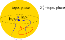
Figure 8: (Color online) Moving a particle (blue) around a loop excitation (red) on the domain wall. The solid line is in the $\mathcal{C}^{4}$ phase. The dashed line is in the $\mathcal{C}_{Z_{2}^{f}}^{4}$ phase.

To do this we consider the process of adiabatically moving a particle $p$ around a pure simple loop $h\in H$ on the domain wall, as shown in Fig. 8. As the pure simple loop is invertible, inserting them will not change the fusion space. But an initial state $|v_{0}\rangle\in F(p)$, after such an adiabatically moving process, can evolve into a different end state $|v_{1}\rangle\in F(p)$. Thus, braiding $p$ around $h$ induces an invertible (since we can always move $p$ backwards) linear map on the fusion space $F(p)$, $\alpha_{p,h}:|v_{0}\rangle\mapsto|v_{1}\rangle$.

Next, consider that we have two particles $p_{1},p_{2}$ in the bulk. If we braid them together (fusing them to one particle $p_{1}\otimes p_{2}$) around the simple loop $h$, we obtain the linear map $\alpha_{p_{1}\otimes p_{2},h}$. If the fusion of the bulk particles is given by $p_{1}\otimes p_{2}=\bigoplus_{i}W_{i}$, we can split $p_{1}\otimes p_{2}$ to the irreducible representations $W_{i}$, and braid $W_{i}$ with $h$. It is easy to see the $\alpha_{p,h}$ maps are automatically compatible with such splitting (or compatible with the embedding intertwiners $W_{i}\to p_{1}\otimes p_{2}$); in other words, $\alpha_{p_{1}\otimes p_{2},h}=\bigoplus_{i}\alpha_{W_{i},h}.$

But it is also equivalent if we move $p_{1},p_{2}$ one after the other. More precisely, we can first separate $p_{2}$ into another 3-disk, braid $p_{1}$ with $h$, and then merge $p_{2}$ back to the original 3-disk. Thus moving $p_{1}$ alone corresponds to the linear map $\alpha_{p_{1},h}\otimes_{\mathbb{C}}\operatorname{id}_{F(p_{2})}$. Similarly, moving $p_{2}$ alone corresponds to $\operatorname{id}_{F(p_{1})}\otimes_{\mathbb{C}}\alpha_{p_{2},h}$ and in total we have the linear map ${\alpha_{p_{1},h}\otimes_{\mathbb{C}}\alpha_{p_{2},h}}$. Therefore, $\alpha_{p_{1}\otimes p_{2},h}=\alpha_{p_{1},h}\otimes_{\mathbb{C}}\alpha_{p_{2},h}$, or using only irreducible representations,

$$\alpha_{p_{1},h}\otimes_{\mathbb{C}}\alpha_{p_{2},h}=\bigoplus_{i}\alpha_{W_{i},h}.$$ (23)

These linear maps are compatible with the fusion of bulk particles.

Figure 9: The fusion of domain wall stringlike excitations $s^{\text{bdry}}_{g_{1}}\otimes s^{\text{bdry}}_{g_{2}}=s^{\text{bdry}}_{g_{1}g_{2}}$ which can be abbreviated as $g_{1}\otimes g_{2}=g_{1}g_{2}$.

Moreover, the pure simple loop $h$ provides such an invertible linear map $\alpha_{p,h}$ for each particle $p\in\mathrm{s}\mathcal{R}\mathrm{ep}(G_{f})$ in $\mathcal{C}^{4}$, thus the set of linear maps $\varphi(h)\equiv\{\alpha_{p,h}\}$ is an automorphism of the super fiber functor, $\varphi(h)\in G_{f}\equiv\operatorname{Aut}(F)$. In other words, we obtain a map $\varphi$ from the pure simple loops $H$ to $G_{f}$, $\varphi:H\to G_{f}$. It is compatible with the fusion of simple loops, because the path of braiding around two concentric simple loops, $g_{1},g_{2}$ (as in Fig. 9), separately, can be continuously deform to the braiding path around the two loops together, or around their fusion $g_{1}\otimes g_{2}=g_{1}g_{2}$. This implies that $\varphi(g_{1})\varphi(g_{2})=\varphi(g_{1}g_{2})$, namely, $\varphi$ is a group homomorphism.

Next we show that $\varphi$ is in fact an isomorphism and $H=G_{f}$. This is a consequence of the following principles:
(1) If an excitation has trivial braiding with the condensed excitations, it must survive as a de-confined excitation in the condensed phase.
(2) there is no nontrivial bulk particle that has trivial half-braiding with all the domain-wall strings.
(1) is a general principle for condensations, while (2) is a remote detectability condition. By the folding trick, we can regard the domain wall as a boundary of the phase ${\mathcal{C}^{4}}\boxtimes{\mathcal{C}_{Z_{2}^{f}}^{4}}$. So we have similar remote detectability condition (2) near the domain wall as that near a boundaryLan et al. (2017a).

A typical half-braiding path is shown in Fig. 8, in the sense that half in $\mathcal{C}^{4}$ and half in $\mathcal{C}_{Z_{2}^{f}}^{4}$. If $\alpha_{p,h}$ is the identity map, it implies trivial half-braiding between the particle $p$ in $\mathcal{C}^{4}$ and simple loop $h$ on the domain wall.

Now, we are ready to show that $\varphi:H\to G_{f}$ is an isomorphism:

1. $\varphi$ is injective. Firstly, the $Z_{2}^{f}$ flux loop, denoted by $z$, which is simple, pure, invertible and survives in the condensed phase $\mathcal{C}_{Z_{2}^{f}}^{4}$, must also be a pure simple loop on the domain wall. Namely, $Z_{2}^{f}\subset H$.

   Consider $\ker\varphi$, namely the pure simple loops that induce just identity linear maps on all particles in $\mathcal{C}^{4}$. On one hand, simple loops in $\ker\varphi$ have trivial half-braiding with all particles in $\mathcal{C}^{4}$. So they also have trivial braiding with the condensed excitations, namely all the bosons in $\mathcal{C}^{4}$. By (1), they should all survive the condensation; in other words, $\ker\varphi$ is at most a subset of pure string excitations in $\mathcal{C}_{Z_{2}^{f}}^{4}$, $\ker\varphi\subset Z_{2}^{f}$. On the other hand, the linear map $\alpha_{p,z}$ induced by the $Z_{2}^{f}$ flux loop $z$ is not the identity map on fermions, so $z\notin\ker\varphi$.

   Therefore, we see that $\ker\varphi$ must be trivial, which means $\varphi$ is injective.

2. $\varphi$ is surjective. We already showed that $\varphi:H\to G_{f}$ is injective, so we can view $H$ as a subgroup of $G_{f}$.

   Now consider a special particle in $\mathcal{C}^{4}$, which carries the representation $\mathrm{Fun}(G_{f}/H)$, linear functions on the right cosets $G_{f}/H$. More precisely, $\mathrm{Fun}(G_{f}/H)$ consists of all linear functions on $G_{f}$, $f:G_{f}\to\mathbb{C}$, such that $f(hx)=f(x),$ $\forall h\in H,x\in G_{f}$ (takes the same value on a coset). The group action is the usual one on functions, ${\rho_{\mathrm{Fun}(G_{f}/H)}(g):f(x)\mapsto f(g^{-1}x)}$.

   The linear maps $\alpha_{p,h}$ induced by the pure simple loops are all actions of group elements in $H$, and they are all identity maps on the special particle $\mathrm{Fun}(G_{f}/H)$. In other words, the bulk particle $\mathrm{Fun}(G_{f}/H)$ has trivial half-braiding with all the pure domain-wall strings. As a non-pure domain-wall string is just the bound state of $f$ with a pure domain-wall string, its half-braiding with $\mathrm{Fun}(G_{f}/H)$ is also trivial. Thus $\mathrm{Fun}(G_{f}/H)$ has trivial half-braiding with all the domain-wall strings. By the remote detectability condition (2), it must be the trivial particle carrying the trivial representation. In other words, we have $G_{f}=H$.

To conclude, the pure simple loop excitations on the domain wall, forms a group under fusion. It is exactly the same group whose representations are carried by the pointlike excitations in the bulk.

V.3 Unitary pointed fusion 2-category with a single invertible fermionic 1-morphism

In addition to the strings on the domain wall discussed above, the domain wall also contain a single fermion with quantum dimension 1. Summarizing the above results, we find that
a 3+1D EF topological order $\mathcal{C}_{EF}^{4}$ has an unique domain wall that connects it to the 3+1D $Z_{2}^{f}$-topological order $\mathcal{C}_{Z_{2}^{f}}^{4}$. The domain wall is described by an unitary pointed fusion 2-category such that for each object (string) there is only one nontrivial invertible 1-morphism corresponding to the fermion.

However, the domain wall only realize a special subset of unitary pointed fusion 2-categories with a single invertible fermionic 1-morphism. The realized fusion 2-categories, denoted as $\mathcal{A}_{w}^{3}$, must also have the following property:

$$Z(\mathcal{A}_{w}^{3})=\mathcal{C}^{4}_{Z_{2}^{f}}\boxtimes(\mathcal{C}^{4}_{Z_{2}^{f}})_{Z(\mathcal{A}_{w}^{3})}^{\text{cen}}.$$ (24)

Here $Z(\mathcal{A}_{w}^{3})$ is the bulk-center of $\mathcal{A}_{w}^{3}$. The notion of the bulk-center was introduced in LABEL:KW1458,KWZ1590 which is a generalization of Drinfeld center to higher categories. Physically, $Z(\mathcal{A}_{w}^{3})$ is the unique 3+1D topological order whose boundary can be $\mathcal{A}_{w}^{3}$. Since $\mathcal{A}_{w}^{3}$ is a domain wall between $\mathcal{C}^{4}_{Z_{2}^{f}}$ and $\mathcal{C}^{4}_{EF}$, after folding, $\mathcal{A}_{w}^{3}$ can viewed as the boundary of the stacked topological order $\mathcal{C}^{4}_{Z_{2}^{f}}\boxtimes{\mathcal{C}^{4}_{EF}}=Z(\mathcal{A}_{w}^{3})$ (strictly speaking we should take time-reversal of one component in the folding trick; but here ${\cal C}^{4}_{Z_{2}^{f}}$ is the same as it time-reversal $\overline{{\cal C}^{4}_{Z_{2}^{f}}}$). Thus $Z(\mathcal{A}_{w}^{3})$ contains $\mathcal{C}^{4}_{Z_{2}^{f}}$ as a subcategory. The centralizer of $\mathcal{C}^{4}_{Z_{2}^{f}}$ in $Z(\mathcal{A}_{w}^{3})$ is given by ${\mathcal{C}^{4}_{EF}}=(\mathcal{C}^{4}_{Z_{2}^{f}})_{Z(\mathcal{A}_{w}^{3})}^{\text{cen}}$, and $Z(\mathcal{A}_{w}^{3})$ happen to be the stacking of $\mathcal{C}^{4}_{Z_{2}^{f}}$ and its centralizer: $Z(\mathcal{A}_{w}^{3})=\mathcal{C}^{4}_{Z_{2}^{f}}\boxtimes(\mathcal{C}^{4}_{Z_{2}^{f}})_{Z(\mathcal{A}_{w}^{3})}^{\text{cen}}$.

VI The unique canonical boundary of 3+1D EF topological orders

Because the fusion 2-category on the domain wall of an EF topological order $\mathcal{C}^{4}_{EF}$ and $Z_{2}^{f}$ topological order $\mathcal{C}^{4}_{Z_{2}^{f}}$ must satisfy the additional condition (24), it is hard to classify such a subset of fusion 2-categories. In this section, we are going to construct the unique canonical boundary for every 3+1D EF topological order, and using the fusion 2-category for such a canonical boundary to classify 3+1D EF topological orders.

To construct the unique canonical boundary for a 3+1D EF topological order $\mathcal{C}^{4}_{EF}$, we start with the unique canonical domain wall $\mathcal{A}_{w}^{3}$ between $\mathcal{C}^{4}_{EF}$ and $\mathcal{C}^{4}_{Z_{2}^{f}}$. We then create a boundary $\mathcal{A}_{Z_{2}}^{3}$ of $\mathcal{C}^{4}_{Z_{2}^{f}}$ by condensing the strings in $\mathcal{C}^{4}_{Z_{2}^{f}}$. As discussed before, such a boundary is described by the SFC $\mathrm{s}\mathcal{R}\mathrm{ep}(Z_{2}^{f})$, viewed as a unitary fusion 2-category.

Figure 10: $\mathcal{A}_{b}^{3}$ is the unique canonical boundary for $\mathcal{C}^{4}_{EF}$. $\mathcal{A}_{b}^{3}$ is formed by stacking the unique canonical domain wall $\mathcal{A}_{w}^{3}$ between $\mathcal{C}^{4}_{EF}$ and $\mathcal{C}^{4}_{Z_{2}^{f}}$, and the boundary $\mathcal{A}^{3}_{Z_{2}^{f}}$ of $\mathcal{C}^{4}_{Z_{2}^{f}}$. Note that $\mathcal{A}_{w}^{3}$ and $\mathcal{A}^{3}_{Z_{2}^{f}}$ is separated by $\mathcal{C}^{4}_{Z_{2}^{f}}$.

The above construction gives rise to an unique canonical boundary for $\mathcal{C}^{4}_{EF}$ (see Fig. 10):

$$\mathcal{A}_{b}^{3}=\mathcal{A}_{w}^{3}\boxtimes_{\mathcal{C}^{4}_{Z_{2}^{f}}}\mathcal{A}_{Z_{2}}^{3}.$$ (25)

Note that the domain wall $\mathcal{A}_{w}^{3}$ has stringlike excitations labeled by $G_{f}$. But the strings labeled by $Z_{2}^{f}\subset G_{f}$ can move across $\mathcal{C}^{4}_{Z_{2}^{f}}$ and then condense on the boundary $\mathcal{A}_{Z_{2}}^{3}$. So the stringlike excitations in the whole boundary $\mathcal{A}_{b}^{3}$ are labeled by $G_{f}/Z_{2}^{f}\equiv G_{b}$. All those strings have quantum dimension 1. Their fusion form the group $G_{b}$. The boundary $\mathcal{A}_{b}^{3}$ also contains an invertible fermion $f$ with quantum dimension 1. Such a pointlike excitation $f$ is inherited from $\mathcal{A}_{Z_{2}}^{3}$, $\mathcal{C}^{4}_{Z_{2}^{f}}$, and $\mathcal{A}_{w}^{3}$. The fermion $f$ can move freely between $\mathcal{A}_{Z_{2}}^{3}$, $\mathcal{C}^{4}_{Z_{2}^{f}}$, and $\mathcal{A}_{w}^{3}$.

We like to mention that a “Majorana chain” (the 1D invertible fermionic topological order Kitaev (2001)) formed by the boundary fermions may attach to the strings discussed above. The Majorana chain is invisible to the braiding between the stings and particles. But it will double the types of strings. The end points of such Majorana chains are the quantum-dimension-$\sqrt{2}$ Majorana zero modes. More detailed discussion about this case will be given later.

Those considerations allow us to obtain the following result (after including the Majorana chain and doubling the string types):
A 3+1D EF topological order $\mathcal{C}_{EF}^{4}$ has an unique boundary $\mathcal{A}_{b}^{3}$. $\mathcal{A}_{b}^{3}$ is described by an unitary fusion 2-category whose objects are labeled by $\hat{G}_{b}$ which is a $Z_{2}^{m}$ extension of $G_{b}$, where $Z_{2}^{m}$ labels the extra Majorana string. The fusion of the objects is described by the group multiplication of $\hat{G}_{b}$. For each object (string) there is one nontrivial invertible 1-morphism corresponding to the fermion. There are also quantum-dimension-$\sqrt{2}$ 1-morphisms (the Majorana zero modes) connecting two objects $g$ and $gm$, with $g\in\hat{G}_{b}$ and $m$ being the generator of $Z_{2}^{m}$.
In LABEL:ZLW, we give explicit constructions and show that all such unitary fusion 2-categories correspond to 3+1D EF topological orders. Classifying such kind of unitary fusion 2-categories give us a classification of 3+1D EF topological orders. We like to remark that $\mathcal{A}_{b}^{3}$ has a form $\mathcal{A}_{b}^{3}=\mathcal{A}_{w}^{3}\boxtimes_{\mathcal{C}^{4}_{Z_{2}^{f}}}\mathcal{A}_{Z_{2}}^{3}$.

The above result allows us to divide the EF topological orders into two groups. If $\hat{G}_{b}=G_{b}\times Z_{2}^{m}$, the corresponding bulk topological orders are called EF1 topological orders. The boundary of EF1 topological orders can be described by a simpler fusion 2-category, since when $\hat{G}_{b}=G_{b}\times Z_{2}^{m}$ we may view the Majorana chain as a trivial string:
A 3+1D EF1 topological order $\mathcal{C}_{EF}^{4}$ has a unique boundary $\bar{\mathcal{A}}_{b}^{3}$, which is described by an pointed unitary fusion 2-category whose objects are labeled by $G_{b}$. The fusion of the objects is described by the group multiplication of $G_{b}$. All 1-morphisms are invertible and fermionic. There is one nontrivial 1-morphism for each object.

If $\hat{G}_{b}$ is a non-trivial extension of $G_{b}$ by $Z_{2}^{m}$, the corresponding bulk topological orders are called EF2 topological orders. In this case, we cannot view the Majorana chain as a trivial string.

VII Classification of EF1 topological orders by pointed unitary fusion 2-categories on the canonical domain wall and boundary

VII.1 The canonical domain wall

In this section we will consider the simple case of classification of EF1 topological orders, which is described by the pointed unitary fusion 2-category $\bar{\mathcal{A}}_{w}^{3}$ on the domain wall. Such fusion 2-categories are special in the sense that their objects (corresponding to pure string types) and simple 1-morphisms are all invertible. The cases with non-invertible 1-morphisms will be discussed later.

We make the following assumptions:

1. The identity (trivial string or trivial particle) related data does not matter. The coherence relations involving both the associator/pentagonator and the identity related data can be viewed as normalization conditions. We can set (by equivalent functors between fusion 2-categories, or physically changing the basis or “gauge”) all the identity related data to be trivial, thus the associator and the pentagonator are properly normalized.

2. There are fermions on the strings, but fermions are not confined to the strings. Instead, fermions can move freely on the domain wall and even to the bulk. As a result, some of the particle related data are fixed by fermionic statistics:

   $$c(f,f)=-1,\quad c(\mathbf{1},\mathbf{1})=c(\mathbf{1},f)=c(f,\mathbf{1})=1.$$ (26)

In short, we assume that there is a convenient “gauge” choice such that some data of $\bar{\mathcal{A}}_{w}^{3}$ are either normalized or fixed by the fermionic statistics.

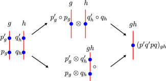
Figure 11: (Color online) The interchange law, corresponding to fusing 4 particles on 2 strings in different orders. The upper path and the lower path differ by a $U(1)$ phase $b(p^{\prime}_{g},q^{\prime}_{h},p_{g},q_{h})$.

Data

1. Objects (pure string types): $G_{f}$, a group that has a $Z_{2}$ central subgroup. The elements of $G_{f}$ label the simple pure strings.

2. 1-morphisms (particles on strings): For any simple pure string labeled by $g\in G_{f}$, we have $\operatorname{Hom}(g,g)=\mathrm{s}\mathcal{V}\mathrm{ec}$. In other words, we have particles live on a string $g$ which is viewed as a defect between the same type-$g$ string. $\operatorname{Hom}(g,g)=\mathrm{s}\mathcal{V}\mathrm{ec}$ corresponds to the degenerate subspace or internal degrees of freedom of the particle. Here, the particle is in general composite, which is formed by accidental degeneracy of bosons and fermion, which in turn gives rise to the super (i.e. $Z_{2}$ graded) vector space $\mathrm{s}\mathcal{V}\mathrm{ec}$. We also have $\operatorname{Hom}(g,h)=0$ for $g\neq h\in G_{f}$. This means that there is no 1D defect between different simple pure strings. Simple 1-morphisms are denoted by $p_{g}\in\operatorname{Hom}(g,g)$, with a subscript to indicate its string type. $p$ values in $\{\mathbf{1},f\}\cong Z_{2}$, and follows a $Z_{2}$ fusion rule.

3. 2-morphisms: linear maps. They correspond to deformation of the particles generated by local operators.

4. Fusion along strings, denoted by $p_{g}\circ p_{g}^{\prime}$ (composition of 1-morphisms, but in fact is the tensor product in $\mathrm{s}\mathcal{V}\mathrm{ec}$). They follow the $Z_{2}$ fusion rule for simple 1-morphisms, $p_{g}\circ p_{g}^{\prime}=(pp^{\prime})_{g}$.

5. Fusion between strings, denoted by $\otimes$, for both objects (given by group multiplication) and 1-morphisms:

   $$g\otimes h =gh,\ \ \ \ g,h\in G_{f}$$

   $$p_{g}\otimes q_{h} =(pq)_{gh}.$$ (27)

   As we assume that particles (1-morphisms) can freely move on the domain wall, the fusion of 1-morphisms along different directions (along or between strings) should be essentially the same, and independent of the string labels.

6. The interchange law, a 2-isomorphism $\tilde{b}(p^{\prime}_{g},q^{\prime}_{h},p_{g},q_{h})\in U(1)$ (see Fig. 11)

   $$(p^{\prime}_{g}\otimes q^{\prime}_{h})\circ(p_{g}\otimes q_{h})\cong(p^{\prime}_{g}\circ p_{g})\otimes(q^{\prime}_{h}\circ q_{h})$$ (28)

   on $(p^{\prime}q^{\prime}pq)_{gh}$. In our case, the simple strings and simple particles are all invertible and have quantum dimension 1. Their degenerate subspaces are always 1-dimensional. Thus the 2-isomorphisms are just $U(1)$ phase factors.

   As particles can be freely detached from strings, we expect the above $U(1)$ phase independent of the string labels. Moreover, if we treat the fusion operations $\circ,\otimes$ as the same one, the difference between the two sides in (28) is just exchanging $q^{\prime}_{h}$ and $p_{g}$. Thus, to be consistent with fermionic statistics, we assume that

   $$\tilde{b}(p^{\prime}_{g},q^{\prime}_{h},p_{g},q_{h})=c(q^{\prime},p).$$ (29)

   

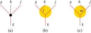
   Figure 12: (Color online) (a) Fusion of strings $g,h,j$ gives rise to a defect between strings $g,h,j$ and string $k$. Two different ways of fusion, (b) and (c), may leads to different defects whose difference in particles is given by $n_{3}(g,h,j)$.

   

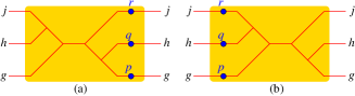
   Figure 13: (Color online) The two domain-wall states in (a) and (b) may differ by a $U(1)$ phase $\tilde{n}_{3}(p_{g},q_{h},r_{j})$ (see (31)).

7. Associator:

   • For $g,h,j\in G_{f}$, we have a 1-morphism ${n_{3}(g,h,j):(g\otimes h)\otimes j\to g\otimes(h\otimes j)}$, valuing in $Z_{2}=\{\mathbf{1},f\}$. See Fig. 12.

   • We also have a 2-isomorphisms $\tilde{n}_{3}(p_{g},q_{h},r_{j})\in U(1)$ to describe the $U(1)$ phase difference between two different orders to fuse strings and particles on the strings (see Fig. 13):

     $$n_{3}(g,h,j)\circ[(p_{g}\otimes q_{h})\otimes r_{j}]$$

     $$\cong[p_{g}\otimes(q_{h}\otimes r_{j})]\circ n_{3}(g,h,j).$$ (30)

     To be consistent with fermionic statistics, we assume that

     $$\tilde{n}_{3}(p_{g},q_{h},r_{j})=c[n_{3}(g,h,j),pqr].$$ (31)

8. Pentagonator: for $g,h,j,k\in G_{f}$, 2-isomorphism $\nu_{4}(g,h,j,k)\in U(1)$:

   $$[\mathbf{1}_{g}\otimes n_{3}(h,j,k)]\circ n_{3}(g,hj,k)\circ[n_{3}(g,h,j)\otimes\mathbf{1}_{k}]$$

   $$\cong n_{3}(g,h,jk)\circ n_{3}(gh,j,k)$$ (32)

Axioms

1. $n_{3}(g,h,j)$ is a normalized 3-cocycle in $H^{3}(G_{f},\mathbb{Z}_{2})$.

2. For $g,h,j,k,l\in G_{f}$,

   $$\tilde{n}_{3}[n_{3}(g,h,j)_{ghj},\mathbf{1}_{k},\mathbf{1}_{l}]\tilde{n}_{3}[\mathbf{1}_{g},n_{3}(h,j,k)_{hjk},\mathbf{1}_{l}]$$ (33)

   $$\ \ \ \ \times\nu_{4}(h,j,k,l)\nu_{4}(g,hj,k,l)\nu_{4}(g,h,j,kl)$$

   $$= \tilde{n}_{3}[\mathbf{1}_{g},\mathbf{1}_{h},n_{3}(j,k,l)_{jkl}]$$

   $$\ \ \ \ \times\nu_{4}(gh,j,k,l)\nu_{4}(g,h,jk,l)\nu_{4}(g,h,j,k).$$

   For convenience, we change the notation a little bit: let $n_{3}(g,h,j)$ value in the additive $\mathbb{Z}_{2}=\{0,1\}$ group instead of the multiplicative $Z_{2}=\{\mathbf{1},f\}$ (where $n=0$ corresponds to the trivial boson $\mathbf{1}$, and $n=1$ corresponds to the non-trivial fermion $f$). Thus,

   $$\tilde{n}_{3}[n_{3}(g,h,j)_{ghj},\mathbf{1}_{k},\mathbf{1}_{l}] =c[n_{3}(g,h,j),n_{3}(ghj,k,l)]$$

   $$=(-1)^{n_{3}(g,h,j)n_{3}(ghj,k,l)},$$ (34)

   and similarly for other $\tilde{n}_{3}$’s. We then have

   $$\frac{\nu_{4}(h,j,k,l)\nu_{4}(g,hj,k,l)\nu_{4}(g,h,j,kl)}{\nu_{4}(gh,j,k,l)\nu_{4}(g,h,jk,l)\nu_{4}(g,h,j,k)}=$$ (35)

   $$(-1)^{n_{3}(g,h,j)n_{3}(ghj,k,l)+n_{3}(g,hjk,l)n_{3}(h,j,k)+n_{3}(g,h,jkl)n_{3}(j,k,l)}.$$

   In other words, the 4-cochain $\nu_{4}(g,h,j,k)$ satisfies

   $$\hskip 1.0pt\mathrm{d}\nu_{4}=(-)^{\mathrm{Sq}^{2}(n_{3})},$$ (36)

   a relation first introduced in LABEL:GW1441, where $\mathrm{Sq}^{2}$ is the Steenrod square and $\nu_{4}$ is normalized.

Here “normalized” means that $n_{3}(g,h,j)=0$, if any of $g,h,k$ is $\mathbf{1}$ and $\nu_{4}(g,h,j,k)=1$, if any of $g,h,j,k$ is $\mathbf{1}$.

We want to point out that by now we considered the consistency conditions only on the domain wall. There are more constraints when we take into account the bulk, namely, the bulk-center of the above fusion 2-category should be $\mathcal{C}_{EF}^{4}\boxtimes\mathcal{C}^{4}_{Z_{2}^{f}}$, in particular the fermion $f$ and the $Z_{2}^{f}$ flux $z$ must be liftable and form the 3+1D $Z_{2}^{f}$-topological order $\mathcal{C}^{4}_{Z_{2}^{f}}$. Unfortunately, we do not have efficient algorithms or theorems to calculate bulk-centers of fusion 2-categories, which makes it difficult to check under what extra conditions the bulk-center of the above fusion 2-category will have the desired form. Instead we will consider the canonical boundary below.

VII.2 The canonical boundary

We know that the $\mathcal{C}^{4}_{Z_{2}^{f}}$ topological order have a gapped boundary by condensing the $Z_{2}^{f}$ flux string $z$. On the gapped boundary there is no string but only one non-trivial particle, the fermion. Imagine we have the gapped domain wall and gapped boundary as above, between them is the intermediate $\mathcal{C}^{4}_{Z_{2}^{f}}$ phase. Now we squeeze the intermediate $\mathcal{C}^{4}_{Z_{2}^{f}}$ phase to a very thin layer, such that we can view the composite domain-wall-$\bar{\mathcal{A}}_{w}^{3}$/$\mathcal{C}^{4}_{Z_{2}^{f}}$/boundary-$\bar{\mathcal{A}}^{3}_{Z_{2}^{f}}$ together as a gapped boundary $\bar{\mathcal{A}}_{b}^{3}$ of $\mathcal{C}_{EF}^{4}$. For such boundary, we only need to check that in its bulk (the bulk-center), the particles form $\mathrm{s}\mathcal{R}\mathrm{ep}(G_{f})$, which is much easier than checking the bulk-center of the domain wall.

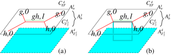
Figure 14: (a) On the domain wall $\bar{\mathcal{A}}_{w}^{3}$, the strings are labeled by $(g,\mu)\in G_{f}$ where $g\in G_{b}$ and $\mu\in\mathbb{Z}_{2}^{f}$. The fusion of strings $(g,\mu)$ and $(h,\nu)$ is given by $(g,\mu)\otimes(h,\nu)=(gh,\mu+\nu+\lambda_{2}(g,h))$. The 2-group-cocycle $\lambda_{2}\in H^{2}(G_{b},\mathbb{Z}_{2}^{f})$ gives rise to an $Z_{2}^{f}$ extension from $G_{b}$ to $G_{f}$. In the above graph, the string $(g,0)$ is represented by a single line (red) and the string $(g,1)$ a double line (red,green), where the extra (green) line can be viewed as the $Z_{2}^{f}$ flux line $z$. (b) Such a $Z_{2}^{f}$ flux line can be canceled by a $Z_{2}^{f}$ flux loop $z$ as indicated by the thick rectangular (blue) loop in the above graph.

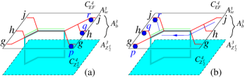
Figure 15: (Color online) The two domain-wall states in (a) and (b) may differ by a $U(1)$ phase $a(p_{g},q_{h},r_{j})$ (see (37)). The string label $(g,0)$ on $\bar{\mathcal{A}}_{w}$ is abbreviated to $g$. This figure shows the case that $e_{2}(g,h)=e_{2}(g,hj)=1,$ ${e_{2}(gh,j)=e_{2}(h,j)=0}$.

The composite boundary is described by a similar fusion 2-category as that for the domain wall. Most of the data and conditions discussed above apply. We only list the difference below:

1. As the $z$ string condenses, the string types on the boundary are now labeled by $G_{b}=G_{f}/Z_{2}^{f}$. At the same time, the 2-cocycle $e_{2}(g,h)\in H^{2}(G_{b},\mathbb{Z}_{2}^{f})$ coming from the extension $Z_{2}^{f}\to G_{f}\to G_{b}$ will arise in other data (see Fig. 14).

2. When fusing $g,h$ on the composite boundary, $e_{2}(g,h)=1$ indicates that there is a $Z_{2}^{f}$ flux loop $z$ along the fused string $gh$ in the intermediate $\mathcal{C}^{4}_{Z_{2}^{f}}$ phase. As a result, the associator $\tilde{n}_{3}(p_{g},q_{h},r_{j})$ needs to be modified. Under certain framing convention (put the particles slightly below the string in Fig. 13 and slightly into the $\mathcal{C}^{4}_{Z_{2}^{f}}$ bulk) we find that (see Fig. 15)

   $$\tilde{n}_{3}(p_{g},q_{h},r_{j})=(-1)^{n_{3}(g,h,j)(p+q+r)}(-1)^{re_{2}(g,h)},$$ (37)

   where $(-1)^{n_{3}(g,h,j)(p+q+r)}$ is the fermion statistics (written in the additive $\mathbb{Z}_{2}$ convention) and $(-1)^{re_{2}(g,h)}$ is the particle-loop statistics coming from $r$ going through the $Z_{2}^{f}$ flux loop $z$ along $gh$.

3. $n_{3}(g,h,j)$ is now a 3-cocycle in $H^{3}(G_{b},\mathbb{Z}_{2})$. The condition for $\nu_{4}$ is then modified to

   $$\frac{\nu_{4}(h,j,k,l)\nu_{4}(g,hj,k,l)\nu_{4}(g,h,j,kl)}{\nu_{4}(gh,j,k,l)\nu_{4}(g,h,jk,l)\nu_{4}(g,h,j,k)}=(-1)^{e_{2}(g,h)n_{3}(j,k,l)}$$

   $$(-1)^{n_{3}(g,h,j)n_{3}(ghj,k,l)+n_{3}(g,hjk,l)n_{3}(h,j,k)+n_{3}(g,h,jkl)n_{3}(j,k,l)}.$$ (38)

   In other words, the 4-cochain $\nu_{4}(g,h,j,k)\in C^{4}(G_{b},U(1))$ satisfies

   $$\hskip 1.0pt\mathrm{d}\nu_{4}=(-)^{n_{3}\underset{{\scriptscriptstyle 1}}{\smile}n_{3}+e_{2}\underset{{\scriptscriptstyle}}{\smile}n_{3}}.$$ (39)

With these one can check that in the bulk-center bosonic particles form representations of $G_{b}$, and fermionic particles form projective representations of $G_{b}$ with class described by $e_{2}$. Together, particles form nothing but $\mathrm{s}\mathcal{R}\mathrm{ep}(G_{f})$. So the above conditions for the composite boundary do give rises to a 3+1D EF topological order. Thus, we have a classification of 3+1D EF1 topological orders by $(G_{b},e_{2},n_{3},\nu_{4})$, where $e_{2}\in H^{2}(G_{b},\mathbb{Z}_{2}),n_{3}\in H^{3}(G_{b},\mathbb{Z}_{2}),\nu_{4}\in C^{4}(G_{b},U(1))$ satisfies (39). The above agrees with the group super-cohomology theory for fermionic SPTs. Recently it was found that fermionic SPTs can have “Majorana chain layer” which is beyond the group super-cohomologyWang and Gu (2017); Kapustin and Thorngren (2017). In next subsection we will show that this “Majorana chain layer” also enters in the classification of topological orders.

For completeness, let us briefly discuss the equivalence relation for the above data. Firstly, $G_{b}$ together with $e_{2}$ is the same data as the group $G_{f}$. Since the particles form $\mathrm{s}\mathcal{R}\mathrm{ep}(G_{f})$, by Tannaka duality $(G_{b},e_{2})$ is fully determined up to group isomorphisms. However, $(n_{3},\nu_{4})$ admits more gauge transformations than co-boundaries: for any 2-cochain $m_{2}\in C^{2}(G_{b},\mathbb{Z}_{2})$ and 3-cochain $\eta_{3}\in C^{3}(G_{b},U(1))$,

$$n_{3} \to n_{3}+\hskip 1.0pt\mathrm{d}m_{2},$$ (40)

$$\nu_{4} \to\nu_{4}\times\hskip 1.0pt\mathrm{d}\eta_{3}\times(-1)^{n_{3}\underset{{\scriptscriptstyle 2}}{\smile}\hskip 1.0pt\mathrm{d}m_{2}+m_{2}\underset{{\scriptscriptstyle}}{\smile}m_{2}+m_{2}\underset{{\scriptscriptstyle 1}}{\smile}\hskip 1.0pt\mathrm{d}m_{2}+e_{2}\underset{{\scriptscriptstyle}}{\smile}m_{2}}.$$

give an equivalent solution. Note that $(-1)^{n_{3}\underset{{\scriptscriptstyle 2}}{\smile}dm_{2}+m_{2}\underset{{\scriptscriptstyle}}{\smile}m_{2}+m_{2}\underset{{\scriptscriptstyle 1}}{\smile}dm_{2}+e_{2}\underset{{\scriptscriptstyle}}{\smile}m_{2}}$ is in general a 4-cochain, and $\hskip 1.0pt\mathrm{d}\nu_{4}$ is shifted under such gauge transformation. If we fix $n_{3}$, namely let $dm_{2}=0$, $m_{2}\in H^{2}(G_{b},\mathbb{Z}_{2})$, $\nu_{4}$ transforms as

$$\nu_{4} \to\nu_{4}\times\hskip 1.0pt\mathrm{d}\eta_{3}\times(-1)^{m_{2}\underset{{\scriptscriptstyle}}{\smile}m_{2}+e_{2}\underset{{\scriptscriptstyle}}{\smile}m_{2}},$$ (41)

where $(-1)^{m_{2}\underset{{\scriptscriptstyle}}{\smile}m_{2}+e_{2}\underset{{\scriptscriptstyle}}{\smile}m_{2}}$ is now a 4-cocycle, but may not be the trivial one. We see that $\nu_{4}$ is in fact classified by (forms a torsor over) the group $H^{4}(G_{b},U(1))/\Gamma$ where $\Gamma$ is the subgroup generated by $(-1)^{m_{2}\underset{{\scriptscriptstyle}}{\smile}m_{2}+e_{2}\underset{{\scriptscriptstyle}}{\smile}m_{2}}$ for all 2-cocycles $m_{2}$. Besides the gauge transformations, different $n_{3},\nu_{4}$ are also equivalent if they can be related by (outer) group isomorphisms of $G_{b}$ (which can be followed by gauge transformations). To “add up” two solutions $(n_{3},\nu_{4})$ and $(n_{3}^{\prime},\nu_{4}^{\prime})$, one also needs to follow a twisted rule,

$$(n_{3},\nu_{4})+(n_{3}^{\prime},\nu_{4}^{\prime})=(n_{3}+n_{3}^{\prime},\nu_{4}\nu_{4}^{\prime}(-1)^{n_{3}\underset{{\scriptscriptstyle 2}}{\smile}n_{3}^{\prime}}).$$ (42)

VIII Classification of EF topological orders by unitary fusion 2-categories on the canonical boundary

VIII.1 Define string type using local or non-local unitary transformations?

In the above discussions we omitted the possibility that between different strings there can be defects/1-morphisms. This is a consequence of defining the type of stringlike excitations up to non-local perturbations along the string (see Sec. III.2). To see this point, let us consider a loop consists of two string segments labeled by $g,h$ connected by two pointlike defects (i.e. 1-morphisms) $\sigma\in\operatorname{Hom}(g,h),\sigma^{\prime}\in\operatorname{Hom}(h,g)$ (see Fig. 16). Under non-local perturbations, the loop can become a $g$ loop carrying $\sigma\circ\sigma^{\prime}\in\operatorname{Hom}(g,g)$, or a $h$ loop carrying $\sigma^{\prime}\circ\sigma\in\operatorname{Hom}(h,h)$. Thus $g$ and $h$ will be equivalent under non-local perturbations along the string.

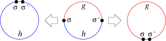
Figure 16: If two strings $g$ and $h$ can be connected by a domain wall (i.e. an 1-morphism), then under non-local unitary transformations, strings $g$ and $h$ will be equivalent.

In the fusion 2-category, the objects/strings and 1-morphisms/point-like defects are actually defined up to local unitary transformations. Moreover, if there exists an invertible 1-morphism (namely a point-like defect with quantum dimension 1) between two objects (namely two string segments), such two objects are equivalent in the fusion 2-category. Therefore, if some $\sigma\in\operatorname{Hom}(g,h)$ is an invertible 1-morphism (i.e. its quantum dimension is 1), then $g$ and $h$ are indeed equivalent as objects in the fusion 2-category, which is consistent with the non-local perturbation point of view. However, it is possible that no 1-morphism in $\operatorname{Hom}(g,h)$ is invertible, and $g,h$ are not equivalent in the fusion 2-category. To include this possibility, we introduce a different equivalent relation of strings, using local unitary transformations plus invertible 1-morphisms, which is consistent with that in the fusion 2-category: Two strings defined under local unitary transformations are called of the same l-type if there is an invertible 1-morphism between them. The set of l-types will be denoted by $\hat{G}_{b}$. We have already shown that the string types defined via non-local unitary transformations form a group $G_{b}$. Clearly $|\hat{G}_{b}|\geq|G_{b}|$, and two different l-types may correspond to the same type.

With the expanded string types defined by local unitary transformation, our arguments in Section V are still valid, which shows that, on the boundary, closed strings have quantum dimension 1 and form a group under fusion. $\hat{G}_{b}$ is actually a group that describes the fusion of the l-types. Also, using the half braiding with the pointlike excitation in the bulk (see Section V), we can assign each boundary string (i.e. each l-type) a group element in $G_{b}$. Thus there is a group homomorphism $\hat{G}_{b}\xrightarrow{\pi^{m}}G_{b}$. If there are non-invertible 1-morphisms between different l-types, they can together form a closed loop and must be assigned to the same element in $G_{b}$. In fact the string types up to non-local perturbations is just l-types further up to non-invertible 1-morphisms. Indeed, $G_{b}$ is a quotient group of $\hat{G}_{b}$ by imposing equivalent relations via non-invertible 1-morphisms.

VIII.2 New string type from Majorana chain

Next we carefully examine what possible non-invertible 1-morphisms can there be and their physical meaning. Since all the l-types of strings labeled by $g\in\hat{G}_{b}$ have quantum dimension 1 and form a group under fusion, the 1-morphisms automatically obtain a grading by this group, namely $p\in\operatorname{Hom}(g,h)$ is graded by $hg^{-1}$. As a result of such grading, the total quantum dimension of non-empty $\operatorname{Hom}(g,h)$ must be the same. In our previous work discussing AB topological orders, $\dim\operatorname{Hom}(g,h)=\dim\operatorname{Hom}(g,g)=1$, thus $\operatorname{Hom}(g,h)$ can only allow one invertible 1-morphism, or be empty; in this case non-empty $\operatorname{Hom}(g,h)$ just implies $g=h$. In other words in AB topological orders there is no room for non-invertible 1-morphisms on the canonical boundary. It also means that on the canonical boundary of AB topological, the string l-types defined using local unitary transformations plus invertible 1-morphisms and the string types defined using non-local unitary transformations are the same, i.e. $\hat{G}_{b}=G_{b}$.

However, for EF topological orders it is not the case. Since $\operatorname{Hom}(g,g)=\mathrm{s}\mathcal{V}\mathrm{ec}$, if $\operatorname{Hom}(g,h)$ is not empty for certain $g,h$, we have $\dim\operatorname{Hom}(g,h)=\dim\operatorname{Hom}(g,g)=\dim(\mathrm{s}\mathcal{V}\mathrm{ec})=2$, which means that there can be one non-invertible 1-morphism with quantum dimension $\sqrt{2}$. In this case $|\hat{G}_{b}|>|G_{b}|$.

We can further fuse a $g^{-1}$ string to this non-invertible 1-morphism between $g,h$, and obtain a non-invertible 1-morphism in $\operatorname{Hom}(gg^{-1},hg^{-1})=\operatorname{Hom}(\mathbf{1},hg^{-1})$. Let such $hg^{-1}\equiv m$ and denote the non-invertible 1-morphism by $\sigma_{m}\in\operatorname{Hom}(\mathbf{1},m)$. It is easy to see that for any string $k$, $\sigma_{m}\otimes\mathbf{1}_{k}$ is a non-invertible 1-morphism in $\operatorname{Hom}(k,mk)$. In fact, such $m$ string generates the kernel of the projection $\pi^{m}:\hat{G}_{b}\to G_{b}$.

We find the following properties of such strings:

1. $m$ is a $Z_{2}$ string, $m^{2}=\mathbf{1}$. Consider fusing two $\sigma_{m}$. We obtain $\sigma_{m}\otimes\sigma_{m}\in\operatorname{Hom}(\mathbf{1},m^{2})$ whose quantum dimension is 2. It can only split as the direct sum of two invertible 1-morphisms. This implies that the $m^{2}$ string and $\mathbf{1}$ are equivalent.

2. $m$ is unique. Suppose that there is another non-invertible $\sigma_{m^{\prime}}\in\operatorname{Hom}(\mathbf{1},m^{\prime}).$ Using the same trick, we see that $\sigma_{m}\otimes\sigma_{m^{\prime}}\in\operatorname{Hom}(\mathbf{1},mm^{\prime})$ is the direct sum of two invertible 1-morphisms. Thus, $mm^{\prime}=\mathbf{1}$. Together with $m^{2}=\mathbf{1}$ we conclude that $m=m^{\prime}$.

3. $m$ is central, $\forall g,mg=gm$. To see this, consider $\mathbf{1}_{g}\otimes\sigma_{m}\otimes\mathbf{1}_{g^{-1}}$ which is a non-invertible 1-morphism in $\operatorname{Hom}(gg^{-1},gmg^{-1})=\operatorname{Hom}(\mathbf{1},gmg^{-1})$. Since $m$ is unique we must have $m=gmg^{-1}$.

Therefore, it is possible to have a $Z_{2}$ string $m$ which can be open on the canonical boundary of EF topological orders. Its end points (non-invertible 1-morphism in $\operatorname{Hom}(\mathbf{1},m)$) have quantum dimension $\sqrt{2}$.

Physically, $m$ string is distinguished from the trivial string under the equivalences generated by local unitary transformations. In other words $m$ string and trivial string have different l-types. $m$ string becomes the same as the trivial string under the equivalences generated by non-local unitary transformations. So $m$ string and trivial string have the same type. This implies that $m$ is a descendant string formed by lower dimensional topological excitations (since it can have boundary). On the boundary of a EF topological order, the only lower dimensional topological excitations are the trivial particles and the fermions. Since there is no topological order in 1D, the trivial particles cannot form any non-trivial strings. On the other hand, the fermions can form topological $p$-wave superconducting chain,Kitaev (2001) called the Majorana chain. Thus the $m$ string must be a Majorana chain. The 1-morphism between $m$ string and trivial string in $\operatorname{Hom}(\mathbf{1},m)$ (i.e. the end point of $m$ string) is the Majorana zero mode at the end of the Majorana chain.

We would like to emphasize here that such extra string $m$ and non-invertible 1-morphism $\sigma_{m}$ are the only remaining possibility beyond the case discussed in the last section. The boundary strings are labeled by a larger group $\hat{G}_{b}$, which is a central $Z_{2}$ extension of $G_{b}$,

$$\{\mathbf{1},m\}\equiv Z_{2}^{m}\to\hat{G}_{b}\stackrel{{\scriptstyle\pi^{m}}}{{\to}}G_{b}.$$

With the enlarged boundary string types and non-invertible 1-morphism, EF topological orders are classified by unitary fusion 2-categories $\mathcal{A}_{b}^{3}$ described in Section VI.

VIII.3 Properties of the unitary fusion 2-categories

Next we discuss in more detail how the extra string $m$ and non-invertible 1-morphism $\sigma_{m}$ will affect the classification results.

Now, strings are labeled by a larger group $\hat{G}_{b}$ on the canonical boundary. But note the fact that the data and conditions not involving $\sigma_{m}$ are not affected at all. This means that we can start with a solution $(\hat{G}_{b},\hat{e}_{2},\hat{n}_{3},\hat{\nu}_{4})$ to (39) with the larger group, and then deal with the additional constraints involving $\sigma_{m}$.

The $\sigma_{m}$ 1-morphism must itself satisfy some additional braiding and fusion constraints. This means that $\hat{\tilde{b}}(\bullet,\bullet,\bullet,\bullet)$ and $\hat{\tilde{n}}_{3}(\bullet,\bullet,\bullet)$ involving $\sigma_{m}$ take different forms. We expect that the results are closely related to the braiding statistics of Ising anyons.

Besides, the strings of l-types $g$ and $gm$ can be “connected” by non-invertible 1-morphisms. This implies, for example, that $\hat{n}_{3}(g,h,j)$ and $\hat{n}_{3}(gm,h,j)$, or $\hat{\nu}_{4}(g,h,j,k)$ and $\hat{\nu}_{4}(g,hm,jm,k)$, etc., are related by $m$ and $\sigma_{m}$. As a result, $\hat{n}_{3}$ and $\hat{\nu}_{4}$ can be factorised, $\hat{n}_{3}=n_{3}+n_{m},\hat{\nu}_{4}={\nu}_{4}\nu_{m}$ where $n_{3},\nu_{4}$ are cochains in $G_{b}=\hat{G}_{b}/Z_{2}^{m}$, and $n_{m},\nu_{m}$ are factors depending on how the $m$ string is attached.

In other words, there is map from the unitary fusion 2-categories $\mathcal{A}_{b}^{3}$ that classify EF topological orders to the pointed unitary fusion 2-categories $\bar{\mathcal{A}}_{b}^{3}$ that classify EF1 topological orders. Such a map sends a unitary fusion 2-category $\mathcal{A}_{n}^{3}$ with objects $\hat{G}_{b}$ to a pointed unitary fusion 2-category $\bar{\mathcal{A}}_{n}^{3}$ with objects $\hat{G}_{b}$, by taking the pointed sub-2-category (ignoring the non-invertible 1-morphisms). Therefore, there is map from EF topological orders to EF1 topological orders, which sends a EF topological order with pointlike excitations described by $\mathrm{s}\mathcal{R}\mathrm{ep}(Z_{2}^{f}\rightthreetimes G_{b})$ to a EF1 topological order with pointlike excitations described by $\mathrm{s}\mathcal{R}\mathrm{ep}(Z_{2}^{f}\rightthreetimes\hat{G}_{b})$. This relation allows us to obtain a EF topological order with pointlike excitations $\mathrm{s}\mathcal{R}\mathrm{ep}(Z_{2}^{f}\rightthreetimes G_{b})$ from a EF1 topological order with pointlike excitations $\mathrm{s}\mathcal{R}\mathrm{ep}(Z_{2}^{f}\rightthreetimes\hat{G}_{b})$ that satisfies certain additional constraints.

We leave the details of the additional constraints involving the non-invertible 1-morphism $\sigma_{m}$ for future work (see LABEL:ZLW). We believe that they are the same as those for fermionic SPTs with the Majorana chain layer.

VIII.4 Majorana zero modes at triple-string intersections

Figure 17: (a) A string configuration in bulk, described by the conjugacy class of a triple $(g_{1}^{f},g_{2}^{f},g_{3}^{f})$ in $G_{f}$. (b) Moving to the boundary, the string configuration turns into one is labeled be three group elements $(g_{1},g_{2},g_{3})$ in $\hat{G}_{b}$.

In the following, we will describe a bulk property that allow us to distinguish the EF1 and EF2 topological orders. In particular we will design a setup which allows us to use the appearance of Majorana zero mode to directly measure the cohomology class of $\rho_{2}$. For simplicity, let us assume $G_{f}$ to Abelian for the time being. In this case, the different types of bulk strings are labeled by $g^{f}\in G_{f}$. In our setup, we first choose a fixed set of trapping potentials that trap a fixed set of strings labeled by $g^{f}\in G_{f}$. Note that the different strings in the set can all be distinguished by their different braiding properties with the pointlike excitations. Then, choosing three strings from such a fixed set, we can form a configuration in Fig. 17a. For Abelian $G_{f}$, one may expect that the degeneracy for the configuration Fig. 17a to be 1. In the following, we will show that, sometimes the configuration Fig. 17a has a 2-fold topological degeneracy. By measuring which triples $g_{1}^{f},g_{2}^{f},g_{3}^{f}$ in the fixed set of strings give rise to 2-fold topological degeneracy, we can determine the cohomology class of $\rho_{2}$ directly.

One may point out that the appearance of 2-fold topological degeneracy is not surprising at all, since the EF topological order with Abelian $G_{f}$ contains an emergent fermion in the bulk that has an unit quantum dimension. Such fermions can form a Majorana chain.Kitaev (2001) Some strings in the fixed set may accidentally carry such a Majorana chain. If one or three strings in the configuration Fig. 17a carry Majorana chain, then the configuration will have a 2-fold topological degeneracy, coming from the two Majorana zero modes at the two intersection points. So it appears that the appearance of 2-fold topological degeneracy in the configurations Fig. 17a is not a universal property. We can remove the 2-fold topological degeneracy by choosing our fixed set of strings properly such that none of the string in the fixed set carry Majorana chain. This indeed can be achieved when $\rho_{2}$ is a coboundary. When $\rho_{2}$ is a non-trivial cocycle, there is an obstruction in determining if a string carries a Majorana chain or not. As a result, no matter how we choose the fixed set of strings, there are always some triples $g_{1}^{f},g_{2}^{f},g_{3}^{f}$ in the fixed set of strings, such that their configurations Fig. 17a have 2-fold topological degeneracies.

How to determine $\rho_{2}$ from the topological degeneracy of the configurations Fig. 17a? We first measure the topological degeneracy Fig. 17a where the three strings are chosen from the fixed set. If there is a 2-fold topological degeneracy, we assign

$$\rho_{2}^{f}(g_{1}^{f},g_{2}^{f})=-1.$$ (43)

If there is no degeneracy, we assign

$$\rho_{2}^{f}(g_{1}^{f},g_{2}^{f})=1.$$ (44)

From the function $\rho_{2}^{f}(g_{1}^{f},g_{2}^{f})$ we can determine the cohomology class of $\rho_{2}\in H^{2}(G_{b},Z_{2}^{m})$.

To see this, we first move the string configuration to the boundary. In this case, the bulk string labeled by $G_{f}$ first have a reduction from $G_{f}\stackrel{{\scriptstyle\pi^{f}}}{{\to}}G_{b}$, and then an extension to $\hat{G}_{b}$. In other words, the bulk string types $g^{f}_{1}$, $g^{f}_{2}$, and $g^{f}_{3}$ in $G^{f}$ change to the boundary string types $g_{1}$, $g_{2}$, and $g_{3}$ in $\hat{G}_{b}$ (see Fig. 17b), which satisfy

$$\pi^{f}(g^{f}_{i})=\pi^{m}(g_{i})\in G_{b},$$ (45)

where $\pi^{f}$ and $\pi^{m}$ are the projections $G_{f}\stackrel{{\scriptstyle\pi^{f}}}{{\to}}G_{b}$ and $\hat{G}_{b}\stackrel{{\scriptstyle\pi^{m}}}{{\to}}G_{b}$.

We note that the elements in $\hat{G}_{b}$ can be labeled as $(g^{b},x)$, $g^{b}\in G_{b}$ and $x\in Z_{2}^{m}$. The multiplication in $\hat{G}_{b}$ is given by

$$(g^{b},x)(h^{b},y)=(g^{b}h^{b},\rho_{2}(g^{b},h^{b})xy)$$ (46)

where $\rho_{2}(g^{b},h^{b})$ is a group 2-cocylce in $H^{2}(G_{b},Z_{2}^{m})$. Thus $g_{i}$ has a form $(g^{b}_{i},x_{i})$ where $g_{i}^{b}=\pi^{f}(g^{f}_{i})$. Here we like to stress that the bulk string $g^{f}_{i}$ only determines the $g^{b}_{i}$ component in the pair $(g^{b}_{i},x_{i})$. Since we move the fixed set of bulk strings to the boundary in a particular way, we obtain a particular $x_{i}$ for each $g^{b}_{i}$. In other words, $x_{i}$ is a function of $g^{b}_{i}$, denoted by

$$x_{i}=x(g^{b}_{i}).$$ (47)

Although the bulk string types satisfy $g^{f}_{1}g^{f}_{2}=g^{f}_{3}$ which leads to $g^{b}_{1}g^{b}_{2}=g^{b}_{3}$, the boundary string types $g_{i}$, as a particular lifting from $G_{b}$ to $\hat{G}_{b}$ may not satisfy $g_{1}g_{2}=g_{3}$. In fact we have

$$[g^{b}_{1},x(g^{b}_{1})][g^{b}_{2},x(g^{b}_{2})] =[g^{b}_{1}g^{b}_{2},\rho_{2}(g^{b}_{1},g^{b}_{2})x(g^{b}_{1})x(g^{b}_{2})]$$

$$=[g^{b}_{3},\tilde{\rho}_{2}(g^{b}_{1},g^{b}_{2})x(g^{b}_{3})]$$ (48)

where

$$\tilde{\rho}_{2}(g^{b}_{1},g^{b}_{2})=\rho_{2}(g^{b}_{1},g^{b}_{2})x(g^{b}_{1})x(g^{b}_{2})x^{-1}(g^{b}_{1}g^{b}_{2}).$$ (49)

When $\tilde{\rho}_{2}(\pi^{f}(g^{f}_{1}),\pi^{f}(g^{f}_{2}))=m$, we have $g_{1}g_{2}=mg_{3}$ and the intersection point will carry a Majorana zero mode. In other words, the boundary configuration Fig. 17b has a 2-fold topological degeneracy if $\tilde{\rho}_{2}(\pi^{f}(g^{f}_{1}),\pi^{f}(g^{f}_{2}))=m$.

Since the boundary configuration Fig. 17b can be a short distance away from the boundary, thus moving to the boundary represents a weak perturbantion. In this case, the boundary configuration Fig. 17b having a 2-fold degeneracy implies that the corresponding bulk configuration Fig. 17a also has a 2-fold degeneracy. In other words

$$\tilde{\rho}_{2}(\pi^{f}(g^{f}_{1}),\pi^{f}(g^{f}_{2}))=\rho_{2}^{f}(g^{f}_{1},g^{f}_{2}).$$ (50)

We see that the cocycle $\tilde{\rho}_{2}$ can be determined by measuring the topological degeneracy for bulk string configurations Fig. 17a. We note that $\tilde{\rho}_{2}$ and $\rho_{2}$ differ by a coboundary (49). Thus, up to a coboundary, $\rho_{2}$ can be determined by measuring the topological degeneracy for bulk string configurations Fig. 17a.

We like to pointed out that even when $G_{f}$ is non-Abelian, a non-trivial $Z_{2}^{m}$ extension $\rho_{2}$ also gives rise the Majorana zero modes for some triple string intersections. But in this case, there are extra topological degenercies on intersections of three strings coming from the non-Abelianness of $G_{f}$. The appearance of topological degenerates does not directly imply the appearance of Majorana zero modes. It is non-trivial to separate which topological degeneracy comes from non-Abelian $G_{f}$ and which comes from Majorana zero modes. However, the similar results also hold for non-Abelian $G_{f}$. In the following, we will describe those results for non-Abelian $G_{f}$, but now from a pure bulk point of view.

Again, the key step is to choose a fixed set of trapping potentials that trap a fixed set of strings labeled by $\chi_{g^{f}}\subset G_{f}$. Here $\chi_{g^{f}}$ is the conjugacy class that contains $g^{f}\in G_{f}$. We stress that the different strings in the set can all be distinguished by their different braiding properties with the pointlike excitations. We call two strings to be equivalent if they have the same brading properties with all the pointlike excitations. Thus the strings in our fixed set are all inequivalent. We also assume our fixed set is complete, in the sense that it contains all inequivalent strings. In other words, the number of strings in the set is equal to the number of conjugacy classes in $G_{f}$.

We note that condensation of the pointlike excitation can also form a stringlike excitation. For example condensation of $Z_{2}$-charges along a chain in a $Z_{2}$ gauge theory can form a stringlike excitation that have trivial braiding with all the pointlike excitations. We call such kind of stringlike excitations descendant stringlike excitations, which all equivalent to trivial string under non-local unitray transformations on the string. The above $Z_{2}$-charge condensed chain has a 2-fold degeneracy since it is like a $Z_{2}$ symmetry breaking state. As a result, the corresponding descendant stringlike excitation has a quantum dimension 2 (and such a quantum-dimension-2 string is equivalent to a trivial string with quantum dimension 1). We point out that our fixed set of strings do not contain strings that only differ by attaching a descendant stringlike excitation, since they are regarded as equivalent.

But each string in the fixed set may carry some additional descendant stringlike excitations. We like to reduce this ambiguity by requiring the strings in the fixed set do not carry descendant strings. This is achieved by replacing each string in the set by its equivalent string that have a minimal quantum dimension. However, this still does not remove all the ambiguity.

When and only when $G_{f}$ has a form $G_{f}=Z_{2}^{f}\times G_{b}$, the following two facts become true: (1) there are bulk fermionic excitations with unit quantum dimension, and (2) the condensation of such fermions only break the $Z_{2}^{f}$ symmetry Klassen and Wen (2015) but not any other symmetries in $G_{b}$. Such fermion condensed chain is nothing but the Majorana chain.Kitaev (2001) The Majorana chain is a descendant string. But amazingly, despite the $Z_{2}^{f}$ symmetry breaking on open Majorana chain, the closed Majorana chain has no ground state degeneracy and the Majorana chain has a quantum dimension 1. Attaching Majorana chain to a string will not change the quantum dimension of the string. So the strings in our fixed set, even after minimizing the quantum dimensions, may still carry Majorana chains. It turns out that there is an obstruction to find a complete set of inequivalent strings that do not carry Majorana chains for EF2 topological orders, while for EF1 topological orders there is no such an obstruction.

To test if the strings in our fixed set carry Majorana chains or not, we choose three strings from our fixed set to form a configuration in Fig. 1. The topological degeneracy of the configuration is calculated in the following way. We first consider a set of pairs that have a form $(\tilde{g}_{1},\tilde{g}_{2})$, where $\tilde{g}_{1}\in\chi_{g^{f}_{1}}$ and $\tilde{g}_{2}\in\chi_{g^{f}_{2}}$. The two pairs $(\tilde{g}_{1},\tilde{g}_{2})$ and $(\tilde{g}_{1}^{\prime},\tilde{g}_{2}^{\prime})$ are equivalent if they are related by

$$\tilde{g}_{1}^{\prime}=h\tilde{g}_{1}h^{-1},\ \ \ \ \tilde{g}_{2}^{\prime}=h\tilde{g}_{2}h^{-1},\ \ \ \ h\in G_{f}.$$ (51)

The number of equivalent classes of the pairs, $N(\chi_{g^{f}_{1}},\chi_{g^{f}_{2}})$, is the topological degeneracy of the configuration in Fig. 1, provided that the three strings do not carry Majorana chains. If one or three strings carry Majorana chains, the topological degenercy of the configuration in Fig. 1 will be given by $2N(\chi_{g^{f}_{1}},\chi_{g^{f}_{2}})$. In this case, we say the triple string intersection in Fig. 1 carry a Majorana zero mode.

Now we introduce a function: $\rho_{2}^{f}(g_{1}^{f},g_{2}^{f})=1$ if the topological degeneracy of the configuration in Fig. 1 is $N(\chi_{g^{f}_{1}},\chi_{g^{f}_{2}})$, and $\rho_{2}^{f}(g_{1}^{f},g_{2}^{f})=-1$ if the topological degeneracy is $2N(\chi_{g^{f}_{1}},\chi_{g^{f}_{2}})$. Clearly $\rho^{f}_{2}$ satisfies

$$\rho^{f}_{2}(g_{1}^{f},g_{2}^{f})=\rho^{f}_{2}(h_{1}g_{1}^{f}h_{1}^{-1},h_{2}g_{2}^{f}h_{2}^{-1}),\ \ h_{1},h_{2}\in G_{f}.$$ (52)

$\rho_{2}^{f}$ in the above is a cocycle in $Z^{2}(G_{f},Z_{2}^{m})$. If $\rho_{2}^{f}$ is a coboundary, we can choose a fixed set of strings such that all the triple string intersections do not carry Majorana zero modes. The corresponding bulk topological order is an EF1 topological order. If $\rho_{2}^{f}$ is a non-trivial cocycle, then for any choice of a fixed set of strings, there are always triple string intersections that carry Majorana zero modes. The correspond bulk topological order is an EF2 topological order.

Figure 18: The splitting of the topological degeneracy as we move string configuration Fig. 1 to wards the canonical boundary. (a) the case for topological degeneracy $N(\chi_{g^{f}_{1}},\chi_{g^{f}_{2}})$. (b) the case for topological degeneracy $2N(\chi_{g^{f}_{1}},\chi_{g^{f}_{2}})$.

The existence of the canonical boundary for a EF topological order requires $\rho^{f}_{2}(g_{1}^{f},g_{2}^{f})$ to be a function on $G_{b}$, i.e. it has a form

$$\rho^{f}_{2}(g_{1}^{f},g_{2}^{f})=\tilde{\rho}_{2}[\pi^{f}(g_{1}^{f}),\pi^{f}(g_{2}^{f})],$$ (53)

where $\tilde{\rho}_{2}\in Z^{2}(G_{b},Z_{2}^{m})$. To understand the above result, we move the string configuration Fig. 1 towards the canonical boundary. The string type will change from the bulk type $\chi_{g^{f}}$ to the boundary l-type $g\in\hat{G}_{b}$: $\chi_{g^{f}}\to g^{b}\to g$ that satisfy

$$g_{b}\in\pi^{f}(\chi_{g^{f}}),\ \ \ \ \ g_{b}=\pi^{m}(g).$$ (54)

The $N(\chi_{g^{f}_{1}},\chi_{g^{f}_{2}})$-fold or $2N(\chi_{g^{f}_{1}},\chi_{g^{f}_{2}})$-fold topological degeneracy will split (see Fig. 18). Note that the 2-fold topological degeneracy from Majorana zero modes is not affected by moving to the boundary. Because of the reduction $\chi_{g^{f}}\to g^{b}$ on the boundary, the Majorana zero modes can only depend on $G_{b}$, and hence $\rho^{f}_{2}(g_{1}^{f},g_{2}^{f})$ is only a function on $G_{b}$. The resulting $\tilde{\rho}_{2}(g^{b}_{1},g_{2}^{b})$ determines the $Z_{2}^{m}$ extension of $G_{b}$.

VIII.5 Necessary conditions for EF2 topological order

From the bulk consideration in the last section, we see that the $\rho_{2}$ characterizing the EF2 topological orders are highly restricted. We focus on the particular $\tilde{\rho}_{2}$ that directly comes from measuring the Majorana zero modes in the bulk; it can differ from $\rho_{2}$ by a coboundary. First, the pullback of $\tilde{\rho}_{2}$ by $G_{f}\xrightarrow{\pi^{f}}G_{b}$ gives us a $\rho^{f}_{2}=(\pi^{f})^{*}\tilde{\rho}_{2}\in H^{2}(G_{f},\mathbb{Z}_{2})$ (see eqn. (50)). Such a pullback must satisfy eqn. (52). This gives us a condition on $\tilde{\rho}_{2}$:

$$\tilde{\rho}_{2}(g_{1}^{b},g_{2}^{b})=\tilde{\rho}_{2}(h_{1}g_{1}^{b}h_{1}^{-1},h_{2}g_{2}^{b}h_{2}^{-1}),\ \ \ \ h_{1},h_{2}\in G_{b}.$$ (55)

In other words, EF2 topological order can exist only when $G_{b}$ has non-trivial 2-cocycles with the above symmetry condition. This is the first necessary conditions for EF2 topological orders. We note that when $G_{b}$ is abelian, the above condition becomes trivial and imposes no constraint.

We also like to point out that a Majorana chain can be attached to a bulk string characterized by the conjugacy class $\chi_{g}$ of $G_{f}$ only when the centralizer group $Z_{g}(G_{f})$ is a trivial $Z_{2}^{f}$ extension. Here $Z_{g}(G_{f})$ is the subgroup that commutes with an element $g$ in the conjugacy class $\chi_{g}$

$$Z_{g}(G_{f})=\{x\in G_{f}|gx=xg\}.$$ (56)

Physically, the bulk string $\chi_{g}$ breaks the “symmetry” of the particles from $G_{f}$ down to $Z_{g}(G_{f})$. If $Z_{g}(G_{f})$ is not a trivial $Z_{2}^{f}$ extension, then a fermion condensation that breaks the $Z_{2}^{f}$ “symmetry” must also break some additional “symmetries”. In this case, we cannot attach Majorana chain to the bulk string $\chi_{g}$, since the Majorana chain corresponds to a fermion condensation that breaks only the $Z_{2}^{f}$ “symmetry”.Klassen and Wen (2015)

Let us introduce a M-function on $G_{f}$

$$M(g)=\begin{cases}0,\text{ $Z_{g}(G_{f})$ is a trivial $Z_{2}^{f}$ extension}\\ 1,\text{ otherwise}\\ \end{cases}$$ (57)

Since

$$Z_{g}(G_{f})=Z_{zg}(G_{f}),$$ (58)

where $z$ is the generator of $Z_{2}^{f}$, we have

$$M(g)=M(zg).$$ (59)

Therefore, we may also view $M$ as a function on $G_{b}$.

Since the bulk string $\chi_{g}$, $g\in G_{f}$, has no ambiguity of Majorana string when $M(g)=1$, we see that $\rho^{f}_{2}$ satisfies

$$\rho^{f}_{2}(g_{1}^{f},g_{2}^{f})=0,\text{ if }M(g_{1}^{f})=M(g_{2}^{f})=M(g_{1}^{f}g_{2}^{f})=1.$$ (60)

This becomes a condition on the $G_{b}$-cocycle $\tilde{\rho}_{2}$

$$\tilde{\rho}_{2}(g_{1}^{b},g_{2}^{b})=0,\text{ if }M(g_{1}^{b})=M(g_{2}^{b})=M(g_{1}^{b}g_{2}^{b})=1.$$ (61)

This is the second necessary conditions for EF2 topological orders. We note that the two conditions (55)(61) are not invariant under adding coboundaries. Physically, on the canonical boundary, unlike in the bulk, it is always possible to attach Majorana chains to strings, since the $G_{f}$ “symmetry” is broken down to $Z_{2}^{f}$ on the boundary. This can change $\rho_{2}$ by arbitrary coboundaries. Thus, generic $\rho_{2}$ may not satisfy (55)(61); we only require (55)(61) for a particular $\tilde{\rho}_{2}$ that is cohomologically equivalent to generic $\rho_{2}$.

As an example, for $G_{f}=Z_{4}^{f}\times G_{b}^{\prime}$, we find $M(g)=1$ for all $g\in Z_{4}^{f}\times G_{b}^{\prime}$. Thus, there is no EF2 topological order with $G_{f}=Z_{4}^{f}\times G_{b}^{\prime}$. In LABEL:LZW, it was shown that 3+1D fermionic $Z_{4}^{f}$-SPT phases from fermion decoration are described by $\mathbb{Z}_{2}$. The above argument shows that there is no Majorana chain decoration for $Z_{4}^{f}$ symmetry. Thus fermion decoration produces all SPT phases, and all 3+1D fermionic $Z_{4}^{f}$-SPT phases are classified by $\mathbb{Z}_{2}$.

IX A general framework for 3+1D topological orders with symmetries

We see that in 3+1D the intrinsic topological orders are closely related to SPT phases. In the above section we showed that the classification of EF topological orders is the same as that of fermionic SPT phases. Without the Majorana chain layer, both EF topological orders and fermionic SPT phases are classified by the group super-cohomology theory; with the Majorana chain layer, also very strong evidence indicates that they have one-to-one correspondence. Combined with our previous results on 3+1D AB topological orders, we conclude that
All 3+1D topological orders correspond to gauged 3+1D SPT phases: AB topological orders correspond to gauged bosonic SPTs and EF topological orders correspond to gauged fermionic SPTs.

The SPT and the topological order are the end points of ungauging/gauging procedures respectively. They are also the two extreme cases with only symmetry no intrinsic topological order and only intrinsic topological order no symmetry. Because of these, it is natural to conjecture that if we partially gauge a SPT or ungauge a topological order, in-between we should get a state with both symmetry and topological order, in other words, a symmetry enriched topological order (SET). Therefore, we expect the following general classification framework for 3+1D topological phases with symmetries:

Different partially gauging procedures, equivalently different subgroup sequences $H_{1}\subset H_{2}\subset\cdots\subset G$, give rise to different sequences of intermediate SETs. The starting point, SPT, and end point, topological order, are fixed. They have one-to-one correspondence between each other, according to our classification results. We believe that in the same gauging sequence the phases share the same classification data. However, their physical interpretations are different at different steps.

In particular, fermionic SETs and topological orders (note that EF topological order is a bosonic topological order with emergent fermionic particles) should be special cases starting from fermionic SPTs but keep the fermion number parity (FNP) not gauged until the last step:

Recall that in 2+1D we classified topological phases with symmetry by a triple of categories $\mathcal{E}\subset\mathcal{C}\subset\mathcal{M}$Lan et al. (2017b, c) where $\mathcal{E}$ is the symmetric category of local excitations and corresponds to the representations of the symmetry group, $\mathcal{E}=\mathcal{R}\mathrm{ep}(G)$ or $\mathcal{E}=\mathrm{s}\mathcal{R}\mathrm{ep}(G_{f})$, $\mathcal{C}$ is the category of all bulk excitation and $\mathcal{M}$ is the gauged theory. In particular for 2+1D SPT phases we have $\mathcal{E}=\mathcal{C}\subset\mathcal{M}$. Now this idea naturally generalizes to 3+1D, since any 3+1D topological order contains a symmetric subcategory $\mathcal{E}$ corresponding to its pointlike excitations, and can be viewed as a gauged SPT $\mathcal{M}$ with symmetry $\mathcal{E}$. A generic 3+1D SET is then described by certain 2-category $\mathcal{C}$ satisfying $\mathcal{E}\subset\mathcal{C}\subset\mathcal{M}$. In the gauging procedures, the modular extension $\mathcal{M}$ remains the same, while $\mathcal{E}$ and $\mathcal{C}$ becomes smaller and larger respectively ($\mathcal{E}=\mathcal{C}=\mathcal{R}\mathrm{ep}(G)$ or $\mathrm{s}\mathcal{R}\mathrm{ep}(G_{f})$ for the SPT phase while $\mathcal{E}$ is trivial and $\mathcal{C}=\mathcal{M}$ for the topological order).

As we already have good understanding about the 3+1D SPT phases, it is thus quite hopeful for a complete understanding of 3+1D topological orders and symmetries by thoroughly studying the (partially) gauging procedures.

We thank Zheng-Cheng Gu for helpful discussions, and Chenjie Wang for sharing his unpublished result about the appearance of Majorana zero modes on linked loops in some 3+1D fermionic SPT states. XGW is supported by NSF Grant No. DMR-1506475 and DMS-1664412. Part of the work was done at Perimeter Institute for Theoretical Physics and Tsinghua University. Research at Perimeter Institute is supported by the Government of Canada through Industry Canada and by the Province of Ontario through the Ministry of Research. TL’s visit at Tsinghua University was supported by Chinese Ministry of Education under grants No.20173080024.

Appendix A Tannaka Duality

Our approach in this paper relies heavily on the Tannaka dualityTannaka (1938), or Tannaka reconstruction theorem for group representations. In this section, we will give a physical introduction of Tannaka duality. In the meantime, we will also introduce and explain some important concepts used in this paper in detail.

A.1 Two physical models

A physical motivation of the Tannaka Duality is the following: let us consider a bosonic or a fermionic system with a symmetry $G$. We assume the ground state to be a product state that does not break the symmetry. If we only measure the system via probes that do not break the symmetry, can we detect the symmetry group of the system? We note that a symmetry transformation acts on objects that break the symmetry (i.e. not invariant under the symmetry transformation). Thus we need to break the symmetry in order to measure the symmetry transformation directly. In contrast, the symmetric probes only produce objects that do not break the symmetry, such as particles trapped by symmetric potential that are described by representations $\rho$ of the symmetry group: $\rho\in$ Rep$(G)$. On the other hand, the symmetric probes do allow us to fuse and braid those symmetric particles in arbitrary ways.

To describe those fusion and braiding processes, the concept of fusion space is important: if the particles are obtained by symmetric trap potentials, then the fusion space ${\cal V}$ is simply the ground state subspace of the total Hamiltonian with traps: $H_{\text{tot}}=H_{0}+\sum_{i}\Delta H_{\text{trap}}(x_{i})$ which trap particles $p_{i}$ at $x_{i}$. We denote the fusion space as ${\cal V}(M,p_{1},p_{2},\cdots)$ where $M$ is the space manifold that supports our system. So the fusion and the braiding processes, as well as the symmetric deformation of the Hamiltonians $H_{0}$ and $\Delta H_{\text{trap}}$, correspond to unitary linear maps on the fusion space. Tannaka duality tells us how to use those symmetric operations, i.e. the linear maps on the fusion space ${\cal V}(M,p_{1},p_{2},\cdots)$, to obtain the symmetry group $G$.

Mathematically, the fusion and braiding, as well as the symmetric deformation of the Hamiltonians $H_{0}$ and $\Delta H_{\text{trap}}$, on all the possible trapped particles form a structure which is denoted as $\mathcal{R}\mathrm{ep}(G)$ if the all the particles are bosons, or as $\mathrm{s}\mathcal{R}\mathrm{ep}(G)$ if the some particles are fermions. Such a structure is called symmetric fusion category (SFC). The particles are labeled by the representations of $G$, which form a set Rep$(G)$. So a SFC $\mathcal{R}\mathrm{ep}(G)$ or $\mathrm{s}\mathcal{R}\mathrm{ep}(G)$ contains the set Rep$(G)$ whose elements are called objects (which correspond to trapped particles). $\mathcal{R}\mathrm{ep}(G)$ or $\mathrm{s}\mathcal{R}\mathrm{ep}(G)$ also contains addition data that describe fusion and braiding of particles in Rep$(G)$. In particular, the fusion of the particles are non-trivial, since the particles are described by the representations of $G$, and the fusion of the representations is non-trivial.

If we just know the set of representations Rep$(G)$, we cannot recover the group $G$. But if we also know all symmetric operations, such as fusion and braiding, as well as the symmetric deformation of the Hamiltonians $H_{0}$ and $\Delta H_{\text{trap}}$; in other words, if we know $\mathcal{R}\mathrm{ep}(G)$ or $\mathrm{s}\mathcal{R}\mathrm{ep}(G)$, then according to Tannaka duality, we can recover the group $G$.

Another physical motivation of the Tannaka Duality is more relevant to this paper. We consider a 3+1D topological order $\mathcal{C}^{4}$. The pointlike excitations in the topological order are bosons or fermions with trivial mutual statistics. Those particles have a non-trivial fusion rule. The fusion and braiding of those particles are also described by a SFC $\mathcal{E}$. Tannaka duality tells us that from $\mathcal{E}$, we can recover a group $G$. Thus each 3+1D topological order contains a hidden group $G$. In this second example, we do not even have a symmetry. All the operations, such as fusion, braiding, and deformation of $H_{0}$ and $\Delta H_{\text{trap}}$, are allowed, as long as they are generated by local interaction. But how can one recover a group from a problem that has no symmetry?

In the first example, we do have symmetry, but we want to recover the symmetry group via the symmetric operations. In the second example, we want to recover the hidden group in 3+1D topological order which has no symmetry. This two problems happen to be the same problem, which is solved by Tannaka duality.

A.2 Tannaka duality I: all boson

A.2.1 Statement of Tannaka duality

For the moment we restrict to an all-boson SFC $\mathcal{E}$. Mathematically, Tannaka duality states that we can reconstruct a group $G$ from SFC $\mathcal{E}$ by the automorphisms of a fiber functor, namely a braided monoidal functor $F$, from $\mathcal{E}$ to the category of vector spaces, $\mathcal{V}\mathrm{ec}$

$$G\equiv\operatorname{Aut}(F:\mathcal{E}\to\mathcal{V}\mathrm{ec}),$$ (62)

and Tannaka duality tells us that

$$\mathcal{E}\cong\mathcal{R}\mathrm{ep}(G).$$ (63)

This is how we find the hidden group in a SFC $\mathcal{E}$.

To understand Tannaka duality let us choose the SFC to be the category formed by the representations of a finite group $\mathcal{R}\mathrm{ep}(G)$. We like to find out what is the automorphisms of a fiber functor $\tilde{G}\equiv\operatorname{Aut}(F:\mathcal{E}\to\mathcal{V}\mathrm{ec})$?

Let us first describe the representation category $\mathcal{R}\mathrm{ep}(G)$:

1. An object in $\mathcal{R}\mathrm{ep}(G)$ is a group representations $p$, which corresponds to a pair $p\equiv(V(p),\rho_{p})$, where $V(p)$ is a vector space equipped with a group action $\rho_{p}:G\to\mathrm{GL}[V(p)]$. The set of objects in $\mathcal{R}\mathrm{ep}(G)$ is formed by all such pairs (i.e. by all the group representations).

2. The morphisms in the SFC $\mathcal{R}\mathrm{ep}(G)$, $p^{\prime}\to p$, correspond to the embedding map $u:V(p^{\prime})\to V(p)$ which commutes with the group action, $\rho_{p}(g)u=u\rho_{p^{\prime}}(g)$. The morphisms allow us to define the notion of simple objects which correspond to irreducible representations.

3. Representations can be “fused” $p_{1}\otimes p_{2}$, which corresponds to taking the tensor product of the vector spaces $V({p_{1}})\otimes_{\mathbb{C}}V({p_{2}})$ and the new group action is $\rho_{p_{1}\otimes p_{2}}(g)=\rho_{p_{1}}(g)\otimes_{\mathbb{C}}\rho_{p_{2}}(g)$:

   $$p_{1}\otimes p_{2}=(V({p_{1}})\otimes_{\mathbb{C}}V({p_{2}}),\rho_{p_{1}}(g)\otimes_{\mathbb{C}}\rho_{p_{2}}(g)).$$ (64)

In this case, we have the forgetful functor that maps a representation category $\mathcal{R}\mathrm{ep}(G)$ to the category of vector spaces $\mathcal{V}\mathrm{ec}$, $F:p\equiv(V(p),\rho_{p})\mapsto V(p)$ (forgetting the group action part), which is called a fiber functor. An automorphisms of such a fiber functor $F$ is a set of unitary maps, $\alpha=\{\alpha_{p}\}$, one map for each $p$ and $\alpha_{p}$ acts on $V(p)$. Such set of maps must be compatible with the fusion rule described above, as well as the morphisms $p^{\prime}\to p:V(p^{\prime})\overset{u}{\to}V(p)$, i.e. satisfying $\alpha_{p}u=u\alpha_{p^{\prime}}$. The set of all those automorphisms form a group

$$\alpha\cdot\alpha^{\prime}=\{\alpha_{p}\}\cdot\{\alpha_{p}^{\prime}\}=\{\alpha_{p}\alpha_{p}^{\prime}\}.$$ (65)

Such a group is the automorphism group, which happen to be $G$:

$$G\cong\operatorname{Aut}(F:\mathcal{R}\mathrm{ep}(G)\to\mathcal{V}\mathrm{ec}).$$ (66)

This is because, to be compatible with the morphisms and the fusion rule, $\alpha_{p}$ has to be $\rho_{p}(h)$ for a certain $h\in G$. In fact, this is how we recover the symmetry group $G$ in the first model.

In the following, we will describe Tannaka’s construction and the above statements, in terms of the two physical models described above, where the particles are described by a SFC $\mathcal{E}$. This way, one may gain a more physical understanding of Tannaka duality.

A.2.2 Irreducible representations from symmetry operations

Before trying to obtain the group, let us try to obtain the irreducible representations of the group first. In general, a particle $p\in\mathcal{E}$ (trapped by a symmetric potential in the first model) corresponds to a representation. But which particles correspond to irreducible representations? To address this question, we start with the fusion space of $p$ with other particles ${\cal V}(M,p,q,\cdots)$. Note that ${\cal V}(M,p,q,\cdots)$ is the ground state subspace of $H_{0}+\Delta H_{\text{trap}}(x_{p})+\Delta H_{\text{trap}}(x_{q})+\cdots$ that traps the particle $p$ at $x_{p}$, particle $q$ at $x_{q}$, etc . By deforming (or deforming while preserving the symmetry for the first model) just $\Delta H_{\text{trap}}(x_{p})$ to $\Delta H_{\text{trap}}^{\prime}(x_{p})$, we may split the ground state degeneracy

$${\cal V}(M,p,q,\cdots)={\cal V}_{1}\oplus{\cal V}_{2}\oplus\cdots.$$ (67)

the new ground state subspace ${\cal V}_{1}$ can be viewed as the fusion space of another particle $p^{\prime}$ at $x_{p}$ with other particles $q,\cdots$, ${\cal V}_{1}={\cal V}(M,p^{\prime},q,\cdots)$. Thus the above splitting of ${\cal V}(M,p,q,\cdots)$ can be rewritten as

$${\cal V}(M,p,q,\cdots)={\cal V}(M,p^{\prime},q,\cdots)\oplus{\cal V}_{2}\oplus\cdots.$$ (68)

Then we say that there is a morphism from $p^{\prime}$ to $p$: $p^{\prime}\to p$. Here, a morphism $p^{\prime}\to p$ can be understood as that the fusion space of $p^{\prime}$, after a proper unitary transformation, is contained in the fusion space of $p$. If we have morphisms in both directions $p^{\prime}\to p$ and $p\to p^{\prime}$, then the fusion space of $p$ is the same as the fusion space of $p^{\prime}$, up to an unitary transformation. If $p^{\prime}\to p$ implies $p\to p^{\prime}$, for all $p^{\prime}$’s, then the fusion space of $p$ is minimal. For the case of the first model, this means that $p$ corresponds to an irreducible representation of the symmetry group. For the second model, we can formally regard $p$ as an irreducible representation of some group $G$. In category theory, we call such a minimal $p$ as a simple object. In this paper, we also call $p$ as a simple particle.

There is always a trivial simple particle denoted by $\mathbf{1}$. It corresponds to local excitations that can be created by local symmetric operators in the first model or local operators in the second model. Its fusion space has a property

$${\cal V}(M,\mathbf{1},p,q,\cdots)\cong{\cal V}(M,p,q,\cdots).$$ (69)

It is not hard to see that the full splitting of the fusion space is given by (see eqn. (68))

$${\cal V}(M,p,q,\cdots)={\cal V}(M,p_{1},q,\cdots)\oplus{\cal V}(M,p_{2},q,\cdots)\cdots$$ (70)

In this case, we say the particle $p$ is a direct sum of particle $p_{1}$, $p_{2}$, etc :

$$p=p_{1}\oplus p_{2}\oplus\cdots.$$ (71)

Physically, it means that the particle $p$ is an accidental degeneracy of particle $p_{1}$, particle $p_{2}$, etc . For example, in the first model, we may have a particle which is an accidental degeneracy of spin-up and spin-down particle. Such a degeneracy becomes required in the presence of $SU(2)$ spin rotation symmetry. In this case, a spin-1/2 particle is a simple particle (i.e. the fusion space cannot be split further). If we break the $SU(2)$ symmetry, then the spin-1/2 particle becomes a composite particle which is a direct sum of two simple particles, a spin-up and a spin-down particles. For the case of the first model, we see that the symmetric operations of deforming $\Delta H_{\text{trap}}(x_{p})$, which correspond to the morphisms in category theory, allow us to define the notion of irreducible representation without using group transformation and other symmetry breaking operations.

A.2.3 Fusion rules of particles

We may view two nearby simple particles $p_{1}$ and $p_{2}$ (i.e. two irreducible representations) as one particle $p_{3}$ (i.e. one representation):

$$p_{1}\otimes p_{2}=p_{3}.$$ (72)

In general $p_{3}$ is no longer a simple particle (i.e. no longer an irreducible representation):

$$p_{1}\otimes p_{2}=p_{3}=p^{\prime}_{1}\oplus p^{\prime}_{2}\oplus\cdots.$$ (73)

Sometimes, the particle types on the right may repeat

$$p_{1}\otimes p_{2}=p^{\prime}_{1}\oplus p^{\prime}_{1}\oplus p^{\prime}_{2}\oplus\cdots=2p^{\prime}_{1}\oplus p^{\prime}_{2}\oplus\cdots.$$ (74)

We may rewrite the above as

$$p_{i}\otimes p_{j}=\bigoplus_{k}N^{ij}_{k}p_{k},$$ (75)

which is called the fusion rule of the (simple) particles. From eqn. (69), we see that the trivial particle $\mathbf{1}$ is the unit of the fusion operation:

$$\mathbf{1}\otimes p=p\otimes\mathbf{1}=p.$$ (76)

Using $N^{ij}_{k}$ we can calculate dimension of the fusion space with $n$ $p_{i}$ particles on $S^{3}$, which has a form

$$\text{dim}{\cal V}(S^{3},p_{i},p_{i},\cdots,p_{i})=\text{dim}{\cal V}(S^{3},p_{i}^{\otimes n})\sim d_{i}^{n}$$ (77)

in the $n\to\infty$ limit. The number $d_{i}$ is called the quantum dimension of the $p_{i}$ particle. One can show that $d_{i}$ is the largest positive eigenvalue of matrix $N_{i}$, where the matrix elements of $N_{i}$ is given by $(N_{i})_{jk}=N^{ij}_{k}$.

For the case of the first example, eqn. (75) correspond to the decomposition of tensor product of irreducible representations. We see that additional information about the symmetry group $G$, the decomposition of tensor product of irreducible representations, can also be obtained from symmetric operations: the fusion of particles (which is realized by bring two symmetric traps together). From $N^{ij}_{k}$, we can even obtain the dimensions of irreducible representations $p_{i}$, which are given by the quantum dimensions $d_{i}$. This in turn determines the number of elements in the symmetry group $G$:

$$\sum_{i\text{ is simple}}d_{i}^{2}=|G|.$$ (78)

We get more information about the group without using any symmetry breaking operations.

A.2.4 Braiding and topological spin of particles

Consider a fusion space ${\cal V}(M,p,q,\cdots)$. If we adiabatically exchange the two particles $p,q$, the resulting fusion space ${\cal V}(M,q,p,\cdots)$ is always isomorphic to the original one, no matter what the manifold $M$ and background particles/strings are. Therefore, we say that there is a braiding morphism $c_{p,q}$ for the fusion $p\otimes q$,

$$c_{p,q}:p\otimes q\cong q\otimes p.$$ (79)

In general we need to specify the exchange path (for example, clockwise or counter-clockwise in 2+1D). But for the above two physical models, braiding is in fact path independent. This is the defining property of SFC, that for all particles $p,q$,

$$c_{q,p}c_{p,q}=\operatorname{id}_{p\otimes q}.$$ (80)

This means that braiding $p$ a whole loop around $q$ is the same as doing nothing, which is equivalent to path independence.

We can also extract the topological spin of simple particle $p$. Given a fusion space ${\cal V}(M,p,\cdots)$, we twist $p$ by $2\pi$, the fusion space then acquires a phase factor $\theta_{p}$, called the topological spin of $p$. It is in fact determined by the braiding $c_{p,p}$. In the case of SFC, $\theta_{p}$ helps to distinguish bosons and fermions

$$\theta_{p}=\begin{cases}\hfill 1,&p\text{ is a boson,}\\ -1,&p\text{ is a fermion.}\end{cases}$$ (81)

A.2.5 Physical realization of fiber functor

The Tannaka duality requires a fiber functor, which associates a vector space $F(p)$ to a particle $p$, such that it realizes the fusion and braidings of particles, in terms of the tensor product and the (trivial) braiding of vector spaces,

$$F(p\otimes q) \cong F(p)\otimes_{\mathbb{C}}F(q),$$

$$F(c_{p,q}) =c_{F(p),F(q)}.$$ (82)

as if $F(p)$ are local Hilbert spaces. Here the braiding for vector spaces is the usual one:

$$c_{V,W}:v\otimes_{\mathbb{C}}w\mapsto w\otimes_{\mathbb{C}}v,\forall v\in V,w\in W.$$ (83)

We note that if a functor preserves the fusion (it is a monoidal functor), whether preserving braiding or not is just a property of the monoidal functor, not an additional structure (like being an Abelian group or not is a property of a group).

We see a necessary condition for the fiber functor to exist is that particles are all bosons with trivial braiding. It turns out that it is also sufficient.

Physically, only the operations on the fusion spaces are measurable (or physical). So the question is, which fusion space should be associated to the particle $p$ in order to have a fiber functor? One might naturally choose the fusion space to be ${\cal V}(S^{3},p)$ (i.e. the fusion space of a particle $p$ on the space of a 3-sphere $S^{3}$). But ${\cal V}(S^{3},p)=\emptyset$ for a non-trivial particle. So we need to add (non-simple) background particles and strings to make the fusion space non-zero for any added particles. The question is what background particles and strings should we insert besides $p$, to get a fusion space satisfying the conditions (82).

It turns out, we do have a special background (non-simple) particle to achieve this. Let’s denote it by $Q$, which has a direct sum decomposition in terms of the simple particles and their quantum dimensions $d_{i}$:

$$Q=\bigoplus_{i}d_{i}p_{i}.$$ (84)

The fusion space ${\cal V}(S^{3},p,Q)$ (no strings) satisfies

$${\cal V}(S^{3},p\otimes q,Q)\cong{\cal V}(S^{3},p,Q)\otimes_{\mathbb{C}}{\cal V}(S^{3},q,Q).$$ (85)

(In the first example, $Q$ is nothing but the reducible representation $\mathrm{Fun}(G)$, all the functions on $G$. It is the regular representation of $G$.) Therefore, we can take

$$F(p)\equiv{\cal V}(S^{3},p,Q).$$ (86)

It preserves fusion by (85) and also braiding (its property but we will not show explicitly here), thus a desired fiber functor.

A.2.6 Automorphism of the fiber functor

Now we have a fiber functor that maps every particle $p$ to a vector space $F(p)={\cal V}(S^{3},p,Q)$. Physically, the vector space $F(p)={\cal V}(S^{3},p,Q)$ is the ground state subspace of a Hamiltonian on $S^{2}$ with two traps: $H_{0}+\Delta H_{p}+\Delta H_{Q}$, where $\Delta H_{Q}$ traps a particular composite particle $Q=\bigoplus_{i}d_{i}p_{i}$ (a particle with accidental degeneracy).

Next we like to describe the automorphism of the fiber functor. An automorphism is a choice of an unitary map on $F(p)={\cal V}(S^{3},p,Q)$ for each particle $p$. We denote those unitary maps by $\alpha_{p}$. So an automorphism corresponds to a set of unitary maps $\alpha\equiv\{\alpha_{p}\}$. But not every set of unitary maps, $\{\alpha_{p}\}$, is an automorphism. An automorphism also needs to preserve all the structures of the fiber functor, and as a result, needs to satisfy many conditions. But what are those conditions?

We have explained that deforming the trap potential $\Delta H_{p}$ (while preserving the symmetry in the first model) may split that fusion space ${\cal V}(S^{3},p,Q)={\cal V}(S^{3},p^{\prime},Q)\oplus\cdots$. This leads to a morphism $p^{\prime}\to p$. Under the fiber functor $F$ which takes a special fusion space, the morphism $p^{\prime}\to p$ gives rise to an embedding map $u:F(p^{\prime})\to F(p)$. An automorphism $\alpha=\{\alpha_{p}\}$ must be compatible with all those embedding maps:

$$u\alpha_{p^{\prime}}=\alpha_{p}u,$$ (87)

or

$$\lx@xy@svg{\hbox{\raise 0.0pt\hbox{\kern 14.08424pt\hbox{\ignorespaces\ignorespaces\ignorespaces\hbox{\vtop{\kern 0.0pt\offinterlineskip\halign{\entry@#!@&&\entry@@#!@\cr&\\&\crcr}}}\ignorespaces{\hbox{\kern-14.08424pt\raise 0.0pt\hbox{\hbox{\kern 0.0pt\raise 0.0pt\hbox{\hbox{\kern 3.0pt\raise 0.0pt\hbox{$\textstyle{F(p^{\prime})\ignorespaces\ignorespaces\ignorespaces\ignorespaces\ignorespaces\ignorespaces\ignorespaces\ignorespaces}$}}}}}}}\ignorespaces\ignorespaces\ignorespaces\ignorespaces{}{\hbox{\lx@xy@droprule}}\ignorespaces\ignorespaces\ignorespaces{\hbox{\kern 19.39905pt\raise 5.54861pt\hbox{{}\hbox{\kern 0.0pt\raise 0.0pt\hbox{\hbox{\kern 3.0pt\hbox{\hbox{\kern 0.0pt\raise-0.46529pt\hbox{$\scriptstyle{\alpha_{p^{\prime}}}$}}}\kern 3.0pt}}}}}}\ignorespaces{\hbox{\kern 38.08424pt\raise 0.0pt\hbox{\hbox{\kern 0.0pt\raise 0.0pt\hbox{\lx@xy@tip{1}\lx@xy@tip{-1}}}}}}{\hbox{\lx@xy@droprule}}{\hbox{\lx@xy@droprule}}\ignorespaces\ignorespaces\ignorespaces\ignorespaces{}{\hbox{\lx@xy@droprule}}\ignorespaces\ignorespaces\ignorespaces{\hbox{\kern 0.0pt\raise-20.0pt\hbox{{}\hbox{\kern 0.0pt\raise 0.0pt\hbox{\hbox{\kern 3.0pt\hbox{\hbox{\kern 0.0pt\raise-1.50694pt\hbox{$\scriptstyle{u}$}}}\kern 3.0pt}}}}}}\ignorespaces{\hbox{\kern 0.0pt\raise-29.5pt\hbox{\hbox{\kern 0.0pt\raise 0.0pt\hbox{\lx@xy@tip{1}\lx@xy@tip{-1}}}}}}{\hbox{\lx@xy@droprule}}{\hbox{\lx@xy@droprule}}{\hbox{\kern 38.08424pt\raise 0.0pt\hbox{\hbox{\kern 0.0pt\raise 0.0pt\hbox{\hbox{\kern 3.0pt\raise 0.0pt\hbox{$\textstyle{F(p^{\prime})\ignorespaces\ignorespaces\ignorespaces\ignorespaces}$}}}}}}}\ignorespaces\ignorespaces\ignorespaces\ignorespaces{}{\hbox{\lx@xy@droprule}}\ignorespaces\ignorespaces\ignorespaces{\hbox{\kern 52.16849pt\raise-20.0pt\hbox{{}\hbox{\kern 0.0pt\raise 0.0pt\hbox{\hbox{\kern 3.0pt\hbox{\hbox{\kern 0.0pt\raise-1.50694pt\hbox{$\scriptstyle{u}$}}}\kern 3.0pt}}}}}}\ignorespaces{\hbox{\kern 52.16849pt\raise-29.5pt\hbox{\hbox{\kern 0.0pt\raise 0.0pt\hbox{\lx@xy@tip{1}\lx@xy@tip{-1}}}}}}{\hbox{\lx@xy@droprule}}{\hbox{\lx@xy@droprule}}{\hbox{\kern-13.31425pt\raise-40.0pt\hbox{\hbox{\kern 0.0pt\raise 0.0pt\hbox{\hbox{\kern 3.0pt\raise 0.0pt\hbox{$\textstyle{F(p)\ignorespaces\ignorespaces\ignorespaces\ignorespaces}$}}}}}}}\ignorespaces\ignorespaces\ignorespaces\ignorespaces{}{\hbox{\lx@xy@droprule}}\ignorespaces\ignorespaces\ignorespaces{\hbox{\kern 19.83905pt\raise-34.67361pt\hbox{{}\hbox{\kern 0.0pt\raise 0.0pt\hbox{\hbox{\kern 3.0pt\hbox{\hbox{\kern 0.0pt\raise-0.6875pt\hbox{$\scriptstyle{\alpha_{p}}$}}}\kern 3.0pt}}}}}}\ignorespaces{\hbox{\kern 38.85423pt\raise-40.0pt\hbox{\hbox{\kern 0.0pt\raise 0.0pt\hbox{\lx@xy@tip{1}\lx@xy@tip{-1}}}}}}{\hbox{\lx@xy@droprule}}{\hbox{\lx@xy@droprule}}{\hbox{\kern 38.85423pt\raise-40.0pt\hbox{\hbox{\kern 0.0pt\raise 0.0pt\hbox{\hbox{\kern 3.0pt\raise 0.0pt\hbox{$\textstyle{F(p)}$}}}}}}}\ignorespaces}}}}\ignorespaces. \textstyle{F(p^{\prime})\ignorespaces\ignorespaces\ignorespaces\ignorespaces\ignorespaces\ignorespaces\ignorespaces\ignorespaces} \scriptstyle{\alpha_{p^{\prime}}} \scriptstyle{u} \textstyle{F(p^{\prime})\ignorespaces\ignorespaces\ignorespaces\ignorespaces} \scriptstyle{u} \textstyle{F(p)\ignorespaces\ignorespaces\ignorespaces\ignorespaces} \scriptstyle{\alpha_{p}} \textstyle{F(p)} \textstyle{F(p^{\prime})\ignorespaces\ignorespaces\ignorespaces\ignorespaces\ignorespaces\ignorespaces\ignorespaces\ignorespaces} \scriptstyle{\alpha_{p^{\prime}}} \scriptstyle{u} \textstyle{F(p^{\prime})\ignorespaces\ignorespaces\ignorespaces\ignorespaces} \scriptstyle{u} \textstyle{F(p)\ignorespaces\ignorespaces\ignorespaces\ignorespaces} \scriptstyle{\alpha_{p}} \textstyle{F(p)}$$ (92)

The map $u$ is an intertwiner. Intertwiners are simply the local (symmetry preserving) operations.

In the first model, $F(p)$ is in general a reducible representation of the symmetry group $G$. When $p^{\prime}$ is a simple particle, all the intertwiners $u$ tell us all different ways to embed irreducible representation $F(p^{\prime})$ into the reducible one $F(p)$. The condition eqn. (92) tells us that $\alpha_{p}$ is block diagonal and fully determined by its components on different simple particles (irreducible representations) $\alpha_{p^{\prime}}$.

The automorphism $\alpha=\{\alpha_{p}\}$ also needs to be compatible with the fusion of particles. We may view two well separated particles $p_{1}$ and $p_{2}$ as a single particle $p_{3}=p_{1}\otimes p_{2}$. The unitary maps $\alpha_{p_{1}}$, $\alpha_{p_{2}}$, and $\alpha_{p_{3}}$ should be related. Since the fusion space from the fiber functor satisfy eqn. (82), we require $\alpha_{p_{3}}$ equals the tensor product of $\alpha_{p_{1}}$ and $\alpha_{p_{2}}$ (up to the isomorphism fixed by the fiber functor eqn. (82)):

$$\lx@xy@svg{\hbox{\raise 0.0pt\hbox{\kern 33.45071pt\hbox{\ignorespaces\ignorespaces\ignorespaces\hbox{\vtop{\kern 0.0pt\offinterlineskip\halign{\entry@#!@&&\entry@@#!@\cr&\\&\crcr}}}\ignorespaces{\hbox{\kern-23.62987pt\raise 0.0pt\hbox{\hbox{\kern 0.0pt\raise 0.0pt\hbox{\hbox{\kern 3.0pt\raise 0.0pt\hbox{$\textstyle{F(p_{1}\otimes p_{2})\ignorespaces\ignorespaces\ignorespaces\ignorespaces\ignorespaces\ignorespaces\ignorespaces\ignorespaces}$}}}}}}}\ignorespaces\ignorespaces\ignorespaces\ignorespaces{}{\hbox{\lx@xy@droprule}}\ignorespaces\ignorespaces\ignorespaces{\hbox{\kern 35.0437pt\raise 5.60583pt\hbox{{}\hbox{\kern 0.0pt\raise 0.0pt\hbox{\hbox{\kern 3.0pt\hbox{\hbox{\kern 0.0pt\raise-0.40807pt\hbox{$\scriptstyle{\alpha_{p_{1}\otimes p_{2}}}$}}}\kern 3.0pt}}}}}}\ignorespaces{\hbox{\kern 67.27156pt\raise 0.0pt\hbox{\hbox{\kern 0.0pt\raise 0.0pt\hbox{\lx@xy@tip{1}\lx@xy@tip{-1}}}}}}{\hbox{\lx@xy@droprule}}{\hbox{\lx@xy@droprule}}\ignorespaces\ignorespaces\ignorespaces\ignorespaces{}{\hbox{\lx@xy@droprule}}\ignorespaces\ignorespaces\ignorespaces{\hbox{\kern 0.0pt\raise-20.0pt\hbox{{}\hbox{\kern 0.0pt\raise 0.0pt\hbox{\hbox{\kern 3.0pt\hbox{\hbox{\kern 0.0pt\raise-1.75pt\hbox{$\scriptstyle{\cong}$}}}\kern 3.0pt}}}}}}\ignorespaces{\hbox{\kern 0.0pt\raise-29.5pt\hbox{\hbox{\kern 0.0pt\raise 0.0pt\hbox{\lx@xy@tip{1}\lx@xy@tip{-1}}}}}}{\hbox{\lx@xy@droprule}}{\hbox{\lx@xy@droprule}}{\hbox{\kern 67.27156pt\raise 0.0pt\hbox{\hbox{\kern 0.0pt\raise 0.0pt\hbox{\hbox{\kern 3.0pt\raise 0.0pt\hbox{$\textstyle{F(p_{1}\otimes p_{2})\ignorespaces\ignorespaces\ignorespaces\ignorespaces}$}}}}}}}\ignorespaces\ignorespaces\ignorespaces\ignorespaces{}{\hbox{\lx@xy@droprule}}\ignorespaces\ignorespaces\ignorespaces{\hbox{\kern 90.90143pt\raise-20.0pt\hbox{{}\hbox{\kern 0.0pt\raise 0.0pt\hbox{\hbox{\kern 3.0pt\hbox{\hbox{\kern 0.0pt\raise-1.75pt\hbox{$\scriptstyle{\cong}$}}}\kern 3.0pt}}}}}}\ignorespaces{\hbox{\kern 90.90143pt\raise-29.5pt\hbox{\hbox{\kern 0.0pt\raise 0.0pt\hbox{\lx@xy@tip{1}\lx@xy@tip{-1}}}}}}{\hbox{\lx@xy@droprule}}{\hbox{\lx@xy@droprule}}{\hbox{\kern-33.45071pt\raise-40.0pt\hbox{\hbox{\kern 0.0pt\raise 0.0pt\hbox{\hbox{\kern 3.0pt\raise 0.0pt\hbox{$\textstyle{F(p_{1})\otimes_{\mathbb{C}}F(p_{2})\ignorespaces\ignorespaces\ignorespaces\ignorespaces}$}}}}}}}\ignorespaces\ignorespaces\ignorespaces\ignorespaces{}{\hbox{\lx@xy@droprule}}\ignorespaces\ignorespaces\ignorespaces{\hbox{\kern 30.19363pt\raise-34.01222pt\hbox{{}\hbox{\kern 0.0pt\raise 0.0pt\hbox{\hbox{\kern 3.0pt\hbox{\hbox{\kern 0.0pt\raise-1.09557pt\hbox{$\scriptstyle{\alpha_{p_{1}}\otimes_{\mathbb{C}}\alpha_{p_{2}}}$}}}\kern 3.0pt}}}}}}\ignorespaces{\hbox{\kern 57.45071pt\raise-40.0pt\hbox{\hbox{\kern 0.0pt\raise 0.0pt\hbox{\lx@xy@tip{1}\lx@xy@tip{-1}}}}}}{\hbox{\lx@xy@droprule}}{\hbox{\lx@xy@droprule}}{\hbox{\kern 57.45071pt\raise-40.0pt\hbox{\hbox{\kern 0.0pt\raise 0.0pt\hbox{\hbox{\kern 3.0pt\raise 0.0pt\hbox{$\textstyle{F(p_{1})\otimes_{\mathbb{C}}F(p_{2})}$}}}}}}}\ignorespaces}}}}\ignorespaces. \textstyle{F(p_{1}\otimes p_{2})\ignorespaces\ignorespaces\ignorespaces\ignorespaces\ignorespaces\ignorespaces\ignorespaces\ignorespaces} \scriptstyle{\alpha_{p_{1}\otimes p_{2}}} \scriptstyle{\cong} \textstyle{F(p_{1}\otimes p_{2})\ignorespaces\ignorespaces\ignorespaces\ignorespaces} \scriptstyle{\cong} \textstyle{F(p_{1})\otimes_{\mathbb{C}}F(p_{2})\ignorespaces\ignorespaces\ignorespaces\ignorespaces} \scriptstyle{\alpha_{p_{1}}\otimes_{\mathbb{C}}\alpha_{p_{2}}} \textstyle{F(p_{1})\otimes_{\mathbb{C}}F(p_{2})} \textstyle{F(p_{1}\otimes p_{2})\ignorespaces\ignorespaces\ignorespaces\ignorespaces\ignorespaces\ignorespaces\ignorespaces\ignorespaces} \scriptstyle{\alpha_{p_{1}\otimes p_{2}}} \scriptstyle{\cong} \textstyle{F(p_{1}\otimes p_{2})\ignorespaces\ignorespaces\ignorespaces\ignorespaces} \scriptstyle{\cong} \textstyle{F(p_{1})\otimes_{\mathbb{C}}F(p_{2})\ignorespaces\ignorespaces\ignorespaces\ignorespaces} \scriptstyle{\alpha_{p_{1}}\otimes_{\mathbb{C}}\alpha_{p_{2}}} \textstyle{F(p_{1})\otimes_{\mathbb{C}}F(p_{2})}$$ (97)

Since $p_{3}=p_{1}\otimes p_{2}=\bigoplus_{i}p^{\prime}_{i}$ and $F(p_{1}\otimes p_{2})\cong\bigoplus_{i}F(p^{\prime}_{i})$, the above can be rewritten as

$$\lx@xy@svg{\hbox{\raise 0.0pt\hbox{\kern 33.45071pt\hbox{\ignorespaces\ignorespaces\ignorespaces\hbox{\vtop{\kern 0.0pt\offinterlineskip\halign{\entry@#!@&&\entry@@#!@\cr&\\&\crcr}}}\ignorespaces{\hbox{\kern-18.79889pt\raise 0.0pt\hbox{\hbox{\kern 0.0pt\raise 0.0pt\hbox{\hbox{\kern 3.0pt\raise 0.0pt\hbox{$\textstyle{\bigoplus_{i}F(p^{\prime}_{i})\ignorespaces\ignorespaces\ignorespaces\ignorespaces\ignorespaces\ignorespaces\ignorespaces\ignorespaces}$}}}}}}}\ignorespaces\ignorespaces\ignorespaces\ignorespaces{}{\hbox{\lx@xy@droprule}}\ignorespaces\ignorespaces\ignorespaces{\hbox{\kern 35.45149pt\raise 6.6304pt\hbox{{}\hbox{\kern 0.0pt\raise 0.0pt\hbox{\hbox{\kern 3.0pt\hbox{\hbox{\kern 0.0pt\raise-1.2696pt\hbox{$\scriptstyle{\bigoplus_{i}\alpha_{p^{\prime}_{i}}}$}}}\kern 3.0pt}}}}}}\ignorespaces{\hbox{\kern 72.10254pt\raise 0.0pt\hbox{\hbox{\kern 0.0pt\raise 0.0pt\hbox{\lx@xy@tip{1}\lx@xy@tip{-1}}}}}}{\hbox{\lx@xy@droprule}}{\hbox{\lx@xy@droprule}}\ignorespaces\ignorespaces\ignorespaces\ignorespaces{}{\hbox{\lx@xy@droprule}}\ignorespaces\ignorespaces\ignorespaces{\hbox{\kern 0.0pt\raise-20.0pt\hbox{{}\hbox{\kern 0.0pt\raise 0.0pt\hbox{\hbox{\kern 3.0pt\hbox{\hbox{\kern 0.0pt\raise-1.75pt\hbox{$\scriptstyle{\cong}$}}}\kern 3.0pt}}}}}}\ignorespaces{\hbox{\kern 0.0pt\raise-29.5pt\hbox{\hbox{\kern 0.0pt\raise 0.0pt\hbox{\lx@xy@tip{1}\lx@xy@tip{-1}}}}}}{\hbox{\lx@xy@droprule}}{\hbox{\lx@xy@droprule}}{\hbox{\kern 72.10254pt\raise 0.0pt\hbox{\hbox{\kern 0.0pt\raise 0.0pt\hbox{\hbox{\kern 3.0pt\raise 0.0pt\hbox{$\textstyle{\bigoplus_{i}F(p^{\prime}_{i})\ignorespaces\ignorespaces\ignorespaces\ignorespaces}$}}}}}}}\ignorespaces\ignorespaces\ignorespaces\ignorespaces{}{\hbox{\lx@xy@droprule}}\ignorespaces\ignorespaces\ignorespaces{\hbox{\kern 90.90143pt\raise-20.0pt\hbox{{}\hbox{\kern 0.0pt\raise 0.0pt\hbox{\hbox{\kern 3.0pt\hbox{\hbox{\kern 0.0pt\raise-1.75pt\hbox{$\scriptstyle{\cong}$}}}\kern 3.0pt}}}}}}\ignorespaces{\hbox{\kern 90.90143pt\raise-29.5pt\hbox{\hbox{\kern 0.0pt\raise 0.0pt\hbox{\lx@xy@tip{1}\lx@xy@tip{-1}}}}}}{\hbox{\lx@xy@droprule}}{\hbox{\lx@xy@droprule}}{\hbox{\kern-33.45071pt\raise-40.0pt\hbox{\hbox{\kern 0.0pt\raise 0.0pt\hbox{\hbox{\kern 3.0pt\raise 0.0pt\hbox{$\textstyle{F(p_{1})\otimes_{\mathbb{C}}F(p_{2})\ignorespaces\ignorespaces\ignorespaces\ignorespaces}$}}}}}}}\ignorespaces\ignorespaces\ignorespaces\ignorespaces{}{\hbox{\lx@xy@droprule}}\ignorespaces\ignorespaces\ignorespaces{\hbox{\kern 30.19363pt\raise-34.01222pt\hbox{{}\hbox{\kern 0.0pt\raise 0.0pt\hbox{\hbox{\kern 3.0pt\hbox{\hbox{\kern 0.0pt\raise-1.09557pt\hbox{$\scriptstyle{\alpha_{p_{1}}\otimes_{\mathbb{C}}\alpha_{p_{2}}}$}}}\kern 3.0pt}}}}}}\ignorespaces{\hbox{\kern 57.45071pt\raise-40.0pt\hbox{\hbox{\kern 0.0pt\raise 0.0pt\hbox{\lx@xy@tip{1}\lx@xy@tip{-1}}}}}}{\hbox{\lx@xy@droprule}}{\hbox{\lx@xy@droprule}}{\hbox{\kern 57.45071pt\raise-40.0pt\hbox{\hbox{\kern 0.0pt\raise 0.0pt\hbox{\hbox{\kern 3.0pt\raise 0.0pt\hbox{$\textstyle{F(p_{1})\otimes_{\mathbb{C}}F(p_{2})}$}}}}}}}\ignorespaces}}}}\ignorespaces. \textstyle{\bigoplus_{i}F(p^{\prime}_{i})\ignorespaces\ignorespaces\ignorespaces\ignorespaces\ignorespaces\ignorespaces\ignorespaces\ignorespaces} \scriptstyle{\bigoplus_{i}\alpha_{p^{\prime}_{i}}} \scriptstyle{\cong} \textstyle{\bigoplus_{i}F(p^{\prime}_{i})\ignorespaces\ignorespaces\ignorespaces\ignorespaces} \scriptstyle{\cong} \textstyle{F(p_{1})\otimes_{\mathbb{C}}F(p_{2})\ignorespaces\ignorespaces\ignorespaces\ignorespaces} \scriptstyle{\alpha_{p_{1}}\otimes_{\mathbb{C}}\alpha_{p_{2}}} \textstyle{F(p_{1})\otimes_{\mathbb{C}}F(p_{2})} \textstyle{\bigoplus_{i}F(p^{\prime}_{i})\ignorespaces\ignorespaces\ignorespaces\ignorespaces\ignorespaces\ignorespaces\ignorespaces\ignorespaces} \scriptstyle{\bigoplus_{i}\alpha_{p^{\prime}_{i}}} \scriptstyle{\cong} \textstyle{\bigoplus_{i}F(p^{\prime}_{i})\ignorespaces\ignorespaces\ignorespaces\ignorespaces} \scriptstyle{\cong} \textstyle{F(p_{1})\otimes_{\mathbb{C}}F(p_{2})\ignorespaces\ignorespaces\ignorespaces\ignorespaces} \scriptstyle{\alpha_{p_{1}}\otimes_{\mathbb{C}}\alpha_{p_{2}}} \textstyle{F(p_{1})\otimes_{\mathbb{C}}F(p_{2})}$$ (102)

The above is the condition for the automorphism $\alpha=\{\alpha_{p}\}$ to be compatible with the fusion which is a data in $\mathcal{R}\mathrm{ep}(G)$.

The set of unitary maps $\alpha=\{\alpha_{p}\}$ that satisfies eqn. (92) and eqn. (102) is called an automorphism of the fiber functor. If $\alpha=\{\alpha_{p}\}$ and $\alpha^{\prime}=\{\alpha_{p}^{\prime}\}$ are two automorphisms, we can show that $\alpha\cdot\alpha^{\prime}\equiv\{\alpha_{p}\alpha_{p}^{\prime}\}$ is also an automorphism. So the automorphisms form a group $G\equiv\operatorname{Aut}(F)$. Such a group corresponds to the symmetry group in the first physical model. We have measured the symmetry group using only symmetric probes. In the second physical model, $G$ is a group associated with the 3+1D topological order. We have shown that every 3+1D topological order is associated with an unique group $G$.

To emphasize the group nature of the automorphisms $\alpha\equiv\{\alpha_{p}\}$, we may instead write $g\equiv\{g_{p}\}\in G\equiv\operatorname{Aut}(F)$. They give rise to the group action on $F(p)$, by $\rho_{p}(g)=g_{p}$.

A.3 Example of Tannaka reconstruction for $\mathcal{R}\mathrm{ep}(Z_{2})$

In this section we illustrate the Tannaka duality with the simplest example, $\mathcal{R}\mathrm{ep}(Z_{2})$. We will follow the general reconstruction procedure, trying to show the flavor of the abstract theorem.

Firstly let’s describe $\mathcal{R}\mathrm{ep}(Z_{2})$ in terms of fusion. There are two irreducible representations of $Z_{2}$: the trivial denoted by $\mathbf{1}$, the non-trivial one denoted by $e$. The fusion rule is

$$\mathbf{1}\otimes\mathbf{1}=\mathbf{1},\ \ \mathbf{1}\otimes e=e\otimes\mathbf{1}=e,\ \ e\otimes e=\mathbf{1}.$$ (103)

The back ground charge is $Q=\mathbf{1}\oplus e$. We find that $F(e)={\cal V}(S^{3},e\otimes Q)={\cal V}(S^{3},e\oplus\mathbf{1})={\cal V}(S^{3},\mathbf{1})={\cal V}(S^{3})=\mathbb{C}$. The ground state on $S^{3}$ is non degenerate, thus $F(e)$ is one dimensional. Similarly, $F(\mathbf{1})$ is one dimensional as well.

When $p$ is composite, $p=\bigoplus_{i}p_{i}$, eqn. (92) tells us that $\alpha_{p}$ is block diagonal

$$\alpha_{p}=\bigoplus_{i}\alpha_{p_{i}},$$ (104)

where $p_{i}$ are simple. Since $F(p_{i})$ for a simple particle is always one dimensional for $\mathcal{R}\mathrm{ep}(Z_{2})$, $\alpha_{\mathbf{1}}$ and $\alpha_{e}$ are just phase factors. Eqn. (102) requires that

$$\alpha_{\mathbf{1}\otimes e}=\alpha_{\mathbf{1}}\otimes_{\mathbb{C}}\alpha_{e}=\alpha_{e}.$$ (105)

Thus $\alpha_{\mathbf{1}}=1$. Eqn. (102) also requires that

$$\alpha_{e\otimes e}=\alpha_{e}\otimes_{\mathbb{C}}\alpha_{e}=\alpha_{\mathbf{1}}=1.$$ (106)

Thus $\alpha_{e}=\pm 1$. The solution $\{\alpha_{\mathbf{1}}=1,\alpha_{e}=1\}$ corresponds to an automorphism, and the solution $\{\alpha_{\mathbf{1}}=1,\alpha_{e}=-1\}$ corresponds to the other automorphism. The composition $\{\alpha_{\mathbf{1}},\alpha_{e}\}\{\alpha_{\mathbf{1}}^{\prime},\alpha_{e}^{\prime}\}=\{\alpha_{\mathbf{1}}\alpha_{\mathbf{1}}^{\prime},\alpha_{e}\alpha_{e}^{\prime}\}$ is the group multiplication, which tells us that $\{\alpha_{\mathbf{1}}=1,\alpha_{e}=1\}$ and $\{\alpha_{\mathbf{1}}=1,\alpha_{e}=-1\}$ form a $Z_{2}$ group.

A.4 Tannaka duality II: with fermions

We proceed to introduce the Tannaka duality for SFC $\mathcal{E}$ which contains fermions. The idea is almost the same: find a fiber functor, calculate the automorphisms of the fiber functor, and we recover the group. But the fiber functor needs to preserve braiding, while in $\mathcal{V}\mathrm{ec}$ there are only bosons. So we have to change the target of the fiber functor to accommodate fermions. The new target category is just the simplest SFC that contains fermions, namely the category of super vector spaces $\mathrm{s}\mathcal{V}\mathrm{ec}$. The fusion part of $\mathrm{s}\mathcal{V}\mathrm{ec}$ is the same as $\mathcal{R}\mathrm{ep}(Z_{2})$. But now the non-trival particle, denoted by $f$ to distinguish from the $\mathcal{R}\mathrm{ep}(Z_{2})$, is a fermion; its braiding is modified:

$$c_{f,f}=-\operatorname{id}_{\mathbf{1}}.$$ (107)

while other braidings remain trivial. It can be understood as vector spaces with a $Z_{2}$ grading. The non-trivial grading corresponds to fermionic degrees of freedom, while the trivial grading corresponds to bosonic degrees of freedom.

So when there are fermions in $\mathcal{E}$, we instead need a super fiber functor

$$F:\mathcal{E}\to\mathrm{s}\mathcal{V}\mathrm{ec},$$ (108)

It can be physically realized the same way using the fusion space ${\cal V}(S^{3},q,Q)$. And we can follow exactly the same procedure introduced in the last subsection to construct a group from automorphisms of the super fiber functor $F$,

$$G_{f}\equiv\operatorname{Aut}(F).$$ (109)

Such a group is slightly different from the bosonic case. Note that there is a special automorphism $z=\{z_{p}\}$,

$$z_{p}=\begin{cases}\hfill\operatorname{id}_{F(p)},&p\text{ is a boson,}\\ -\operatorname{id}_{F(p)},&p\text{ is a fermion.}\end{cases}$$ (110)

$z$ corresponds to the fermion number parity and commutes with all other automorphisms. Let $Z_{2}^{f}\equiv\{1,z\}$. We see that the group $G_{f}$ must contain $Z_{2}^{f}$ as a central subgroup. We then have

$$\mathcal{E}\cong\mathrm{s}\mathcal{R}\mathrm{ep}(G_{f}).$$ (111)

Where $\mathrm{s}\mathcal{R}\mathrm{ep}(G_{f})$ is constructed similarly like $\mathcal{R}\mathrm{ep}(G)$. They have the same fusion; only the braiding between two fermions has an extra $-1$. In this sense we have $\mathrm{s}\mathcal{V}\mathrm{ec}=\mathrm{s}\mathcal{R}\mathrm{ep}(Z_{2}^{f})$.

A.5 (Super) fiber functor from condensation

In the above we realized the (super) fiber functor using the fusion space on $S^{3}$ with a special background particle $Q$. But we gave no proof why such fusion space preserves the fusion and braiding. In this subsection we give a physical reason why such $Q$ is so special.

In the all-boson case, imagine that we let $Q$ condense to form a new phase, a $Q$-sea, such that $Q$ becomes the trivial particle in the $Q$-sea. One expects the fusion space to remain the same,

$${\cal V}(S^{3},p,Q) ={\cal V}(S^{3},p,\text{trivial particle above }Q\text{-sea})$$

$$={\cal V}(S^{3},p,Q\text{-sea}).$$ (112)

So the properties of ${\cal V}(S^{3},p,Q)$ in fact follows from those of the $Q$-sea, as in ${\cal V}(S^{3},p,Q\text{-sea})$, the particle $p$ behaves like a particle above the $Q$-sea. Then it is clear that we want the $Q$-sea to be a trivial phase, whose particles are described by $\mathcal{V}\mathrm{ec}$.

If there are fermions, similarly we want a condensate whose particles form $\mathrm{s}\mathcal{V}\mathrm{ec}$. But $Q$ should become, instead of the trivial particle, a direct sum $\mathbf{1}\oplus f$, from whose fusion space we can extract both bosonic and fermionic degrees of freedom. It turns out $Q$ should be of the following form:

$$Q=Q_{b}\oplus Q_{f},\quad\dim(Q_{b})=\dim(Q_{f}),$$ (113)

where $Q_{b}$ and $Q_{f}$ are bosonic and fermionic parts respectively. We condense the bosonic part $Q_{b}$, and particles above the $Q_{b}$-sea should be $\mathrm{s}\mathcal{V}\mathrm{ec}$,

$${\cal V}(S^{3},p,Q) ={\cal V}(S^{3},p,\mathbf{1}\oplus f\text{ above }Q_{b}\text{-sea}).$$ (114)

It is indeed from these requirements on the condensation how we determine the special particle $Q$. This idea of condensation is also the main physical motivation of this paper.

Appendix B Relation between emergent Majorana zero modes for linked loops and the 2-cocycle $\rho_{2}$

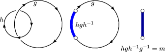
Figure 19: Fuse $h$ loop to the linked $g$ loop on the canonical domain wall. When $hgh^{-1}=gm$ two Majorana zero modes are supported. Further fusing the two segments we obtain an open Majorana chain.

In LABEL:CJWang, it was pointed out that, for some fermionic SPT states, certain linked loops of symmetry twists can carry a pair of Majorana zero modes (see Fig. 19). In this section, we like to discuss a relation between such emergent Majorana zero modes and the non-trivial two cocycle $\rho_{2}$ that characterize the EF2 topological orders. For simplicity, we assume $G_{f}$ to be Abelian. We will show that certain linked looplike excitations in a EF2 topological order carry a pair of Majorana zero modes, one for each linked loop. In other words, certain pairs of looplike excitations carry two-fold topological degeneracy when they are linked and no degeneracy when they are not linked. Such a topological degeneracy is highly non-local in the sense that the degeneracy is shared between the two well separated linked loops. The new result here is that the appearance of Majorana zero modes for linked loops is directly related to the non-trivial $Z_{2}^{m}$ extension of $G_{b}$ on the canonical boundary.

To see the above result, we consider a pair of linked loops in the bulk in Fig. 19. We know that a pair of linked loops in the bulk is characterized by a pair of commuting elements $h^{f},g^{f}$ in $G_{f}$ (assuming $G_{f}$ is non-Abelian for the moment). (To be more precise, a pair of linked loops is characterized by the conjugacy class of a pair of commuting elements $h^{f},g^{f}$.) As we go around a loop, the string labeled by $g^{f}$ is changed into the string labeled by $h^{f}g^{f}(h^{f})^{-1}$. The string can form a loop only when $g^{f}=h^{f}g^{f}(h^{f})^{-1}$. It is why $h^{f},g^{f}$ describing linked loops must commute.

Now, let us assume $G_{f}$ is Abelain. We like to compute the degeneracy for the linked loops in Fig. 19. For Abelian $G_{f}$, all the pointlike excitations and stringlike excitations have an unit quantum dimension. Thus one may expect that degeneracy for the linked loops to be 1. In the following, we like to show that some times the degeneracy can be 2. To obtain such a result, we bring the linked loops to the boundary. This reduces the group elements $h^{f},g^{f}$ in $G_{f}$ to the group elements $h^{b}=\pi^{f}(h^{f}),\ g^{b}=\pi^{f}(g^{f})$ in $G_{b}$ via the natural reduction $G_{f}\stackrel{{\scriptstyle\pi^{f}}}{{\to}}G_{b}=G_{f}/Z_{2}^{f}$. In addition to the reduction $G_{f}\to G_{b}$, there is also an extension $G_{b}\to\hat{G}_{b}$. So the linked loops on the boundary are actually described by $h,g$ in $\hat{G}_{b}$, where $h^{b}=\pi^{m}(h),\ g^{b}=\pi^{m}(g)$ under the projection $\hat{G}_{b}\stackrel{{\scriptstyle\pi^{m}}}{{\to}}G_{b}$. To summarize, the bulk string types $h^{f},g^{f}$ turn to boundary string l-types $h,g$ that satisfy the following relation

$$\pi^{f}(g^{f})=\pi^{m}(g),\ \ \ \ \ \pi^{f}(h^{f})=\pi^{m}(h).$$ (115)

This is the situation described in Fig. 19. As we go around a loop, boundary string labeled by $g$ turns into a boundary string $hgh^{-1}$. Even though $h^{b},g^{b}$ commute in $G_{b}$, their lifts $h,g$ may not commute in $\hat{G}_{b}$, when $\hat{G}_{b}$ is a non-trivial $Z_{2}^{m}$ extension of $G_{b}$. If $h,g$ do not commute, we will have $hgh^{-1}=gm$ where $m$ generates $Z_{2}^{m}$. As a result, there are two pointlike defects between $g$ and $gm$ boundary strings, corresponding to two Majorana zero modes which lead to a 2-fold degeneracy.

To see which linked loops described by $h^{f},g^{f}$ have Majorana zero modes, we first note that the elements in $\hat{G}_{b}$ can be labeled as $(g^{b},x)$, $g^{b}\in G_{b}$ and $x\in Z_{2}^{m}$. The multiplication in $\hat{G}_{b}$ is given by

$$(g^{b},x)(h^{b},y)=(g^{b}h^{b},\rho_{2}(g^{b},h^{b})xy)$$ (116)

where $\rho_{2}(g^{b},h^{b})$ is the group 2-cocycle in $H^{2}(G_{b},Z_{2}^{m})$. For $h^{f},g^{f}$, we have $h=(\pi^{f}(h^{f}),y),g=(\pi^{f}(g^{f}),x)\in\hat{G}_{b}$. As shown in Fig. 19, their commutator $[h,g]\equiv hgh^{-1}g^{-1}=hg(gh)^{-1}$ determines the appearance of Majorana zero modes. Without losing generality, we may assume that $\rho_{2}$ is a normalized 2-cocycle, namely $\rho_{2}(1,g^{b})=\rho_{2}(g^{b},1)=1$, $\forall g^{b}\in G_{b}$. Using the fact that $hg=[h,g]gh$ and $\pi^{f}(h^{f})\pi^{f}(g^{f})=\pi^{f}(g^{f})\pi^{f}(h^{f})$, it is easy to compute $[h,g]=(1,\rho_{2}(\pi^{f}(h^{f}),\pi^{f}(g^{f}))\rho_{2}(\pi^{f}(g^{f}),\pi^{f}(h^{f})))$. We see that the linked loops $h^{f},g^{f}$ have Majorana zero modes when $\rho_{2}(\pi^{f}(h^{f}),\pi^{f}(g^{f}))\rho_{2}(\pi^{f}(g^{f}),\pi^{f}(h^{f}))=m$. The appearance of Majorana zero modes for certain linked loops can detect a certain type of non-trivial $Z_{2}^{m}$ extensions, i.e. those with non-trivial $\rho_{2}(\pi^{f}(h^{f}),\pi^{f}(g^{f}))\rho_{2}(\pi^{f}(g^{f}),\pi^{f}(h^{f}))$ for certain pairs of elements $h^{f},g^{f}$ in $G_{f}$.

References

- Lan et al. (2017a) Tian Lan, Liang Kong, and Xiao-Gang Wen, “A classification of 3+1d bosonic topological orders (i): the case when point-like excitations are all bosons,” (2017a), arXiv:1704.04221 .
- Wen (2013) Xiao-Gang Wen, “Classifying gauge anomalies through spt orders and and classifying gravitational anomalies through topological orders,” Phys. Rev. D 88, 045013 (2013), arXiv:1303.1803 .
- Zhu et al. (2018) Chenchang Zhu, Tian Lan, and Xiao-Gang Wen, To appear (2018).
- Kitaev (2001) A. Y. Kitaev, “Unpaired Majorana fermions in quantum wires,” Phys.-Usp. 44, 131 (2001), cond-mat/0010440 .
- Gu and Wen (2014) Zheng-Cheng Gu and Xiao-Gang Wen, “Symmetry-protected topological orders for interacting fermions – fermionic topological non-linear sigma-models and a group super-cohomology theory,” Phys. Rev. B 90, 115141 (2014), arXiv:1201.2648 .
- Levin and Wen (2005) Michael Levin and Xiao-Gang Wen, “String-net condensation: A physical mechanism for topological phases,” Phys. Rev. B 71, 045110 (2005), cond-mat/0404617 .
- Moradi and Wen (2015) Heidar Moradi and Xiao-Gang Wen, “Universal topological data for gapped quantum liquids in three dimensions and fusion algebra for non-abelian string excitations,” Phys. Rev. B 91, 075114 (2015), arXiv:1404.4618 .
- Wang and Wen (2015) Juven Wang and Xiao-Gang Wen, “Non-abelian string and particle braiding in topological order - modular sl(3,z) representation and 3+1d twisted gauge theory,” Phys. Rev. B 91, 035134 (2015), arXiv:1404.7854 .
- Kapustin (2014) A. Kapustin, “Bosonic Topological Insulators and Paramagnets: A view from cobordisms,” (2014), arXiv:1404.6659 .
- Kong and Wen (2014) Liang Kong and Xiao-Gang Wen, “Braided fusion categories, gravitational anomalies, and the mathematical framework for topological orders in any dimensions,” (2014), arXiv:1405.5858 .
- Freed (2014) D. S. Freed, “Short-range entanglement and invertible field theories,” (2014), arXiv:1406.7278 .
- Kong et al. (2017) Liang Kong, Xiao-Gang Wen, and Hao Zheng, “Boundary-bulk relation in topological orders,” Nucl. Phys. B 922, 62–76 (2017), arXiv:1702.00673 .
- Levin and Wen (2003) Michael Levin and Xiao-Gang Wen, “Fermions, strings, and gauge fields in lattice spin models,” Phys. Rev. B 67, 245316 (2003), cond-mat/0302460 .
- von Keyserlingk et al. (2013) C. W. von Keyserlingk, F. J. Burnell, and S. H. Simon, “Three-dimensional topological lattice models with surface anyons,” Phys. Rev. B 87, 045107 (2013), arXiv:1208.5128 .
- Wen (2017) Xiao-Gang Wen, “Exactly soluble local bosonic cocycle models, statistical transmutation, and simplest time-reversal symmetric topological orders in 3+1d,” Phys. Rev. B 95, 205142 (2017), arXiv:1612.01418 .
- Levin (2013) M. Levin, “Protected edge modes without symmetry,” Phys. Rev. X 3, 021009 (2013), arXiv:1301.7355 .
- Kong (2014) L. Kong, “Anyon condensation and tensor categories,” Nuclear Physics B 886, 436–482 (2014), arXiv:1307.8244 [cond-mat.str-el] .
- Note (1) Without such background particle, the fusion space would be 0 if is a fermion.
- Kong et al. (2015) L. Kong, X.-G. Wen, and H. Zheng, “Boundary-bulk relation for topological orders as the functor mapping higher categories to their centers,” (2015), arXiv:1502.01690 .
- Wang and Gu (2017) Q.-R. Wang and Z.-C. Gu, “Towards a complete classification of fermionic symmetry protected topological phases in 3D and a general group supercohomology theory,” (2017), arXiv:1703.10937 .
- Kapustin and Thorngren (2017) Anton Kapustin and Ryan Thorngren, “Fermionic SPT phases in higher dimensions and bosonization,” J. High Energy Phys. 2017, 80 (2017), arXiv:1701.08264 .
- Klassen and Wen (2015) Joel Klassen and Xiao-Gang Wen, “Topological degeneracy (majorana zero-mode) and 1+1d fermionic topological order in a magnetic chain on superconductor via spontaneous symmetry breaking,” Journal of Physics: Condensed Matter 27, 405601 (2015), arXiv:1412.5985 .
- Lan et al. (2018) Tian Lan, Chenchang Zhu, and Xiao-Gang Wen, To appear (2018).
- Lan et al. (2017b) Tian Lan, Liang Kong, and Xiao-Gang Wen, “Modular Extensions of Unitary Braided Fusion Categories and 2+1D Topological/SPT Orders with Symmetries,” Commun. Math. Phys. 351, 709–739 (2017b), arXiv:1602.05936 .
- Lan et al. (2017c) Tian Lan, Liang Kong, and Xiao-Gang Wen, “Classification of (2+1)-dimensional topological order and symmetry-protected topological order for bosonic and fermionic systems with on-site symmetries,” Phys. Rev. B 95, 235140 (2017c), arXiv:1602.05946 .
- Tannaka (1938) Tadao Tannaka, “Über den Dualitiätssatz der nichtkommutativen topologischen Gruppen,” Tohoku Math. J. 45, 1–12 (1938).
- Note (2) In mathematical formulation of fusion categories, this morphism is only an embedding morphism; generic morphisms are generated by linear combinations, compositions, taking Hermitian conjugates of these embeddings. But in physics we always (secretly) assume linearity and unitarity (including taking Hermitian conjugates of morphisms). So taking only the embedding as our (basis) morphism suffices for our purpose.
- Wang (2017) Chen-Jie Wang, Private communication (2017).