Stochastic Successive Convex Optimization for Two-timescale Hybrid Precoding in Massive MIMO

Abstract

Hybrid precoding, which consists of an RF precoder and a baseband precoder, is a popular precoding architecture for massive MIMO due to its low hardware cost and power consumption. In conventional hybrid precoding, both RF and baseband precoders are adaptive to the real-time channel state information (CSI). As a result, an individual RF precoder is required for each subcarrier in wideband systems, leading to high implementation cost. To overcome this issue, two-timescale hybrid precoding (THP), which adapts the RF precoder to the channel statistics, has been proposed. Since the channel statistics are approximately the same over different subcarriers, only a single RF precoder is required in THP. Despite the advantages of THP, there lacks a unified and efficient algorithm for its optimization due to the non-convex and stochastic nature of the problem. Based on stochastic successive convex approximation (SSCA), we propose an online algorithmic framework called SSCA-THP for general THP optimization problems, in which the hybrid precoder is updated by solving a quadratic surrogate optimization problem whenever a new channel sample is obtained. Then we prove the convergence of SSCA-THP to stationary points. Finally, we apply SSCA-THP to solve three important THP optimization problems and verify its advantages over existing solutions.

I Introduction

Massive MIMO can significantly improve the spectrum efficiency of wireless systems. The conventional fully digital precoding requires one RF chain for each antenna, and thus induces huge hardware cost and power consumption for massive MIMO. As a result, hybrid precoding, where a high-dimensional RF precoder is connected to a low-dimensional baseband precoder with a limited number of RF chains, has been proposed to reduce the hardware cost and power consumption of massive MIMO base station (BS).

The early works on this topic focus on studying fast-timescale hybrid precoding (FHP), where both RF and baseband precoders are adaptive to the real-time channel state information (CSI). For example, in [1], a sparse precoding and combining algorithm based on orthogonal matching pursuit is proposed for single-user mmWave systems. In [2], a low-complexity FHP scheme for multiuser massive MIMO systems is proposed. A limited feedback hybrid precoding scheme is also proposed in [3] for multi-user mmWave systems. One disadvantage of FHP is that the number of RF precoders has to increase with the number of subcarriers in wideband systems such as orthogonal frequency-division multiple access (OFDMA) system (since the CSI is different on different subcarriers), leading to high implementation cost [4, 5]. Moreover, as the real-time full CSI is required at the BS, the CSI signaling overhead is large.

To overcome the above disadvantages of FHP, a two-timescale hybrid precoding (THP) scheme is proposed in [6, 7]. In THP, the RF precoder is adaptive to the channel statistics to achieve the array gain, and the baseband precoder is adaptive to the low-dimensional effective channel to achieve the spatial multiplexing gain. THP has several advantages. Since the channel statistics are approximately the same on different subcarriers [8], THP only needs one RF precoder to cover all subcarriers, which significantly reduces the hardware cost. Moreover, THP reduces the CSI signaling overhead because it does not require knowledge of the real-time high-dimensional CSI. Therefore, THP can achieve a better tradeoff between the implementation cost and performance, making it more attractive in practice [4, 5].

The optimal THP design depends on the RF precoding structure and the specific application scenario. There are two major RF precoding structures: the fully-connected structure where each antenna is connected to all the RF chains, and the partially-connected structure where each antenna is only connected to a single RF chain [9]. For each structure, there are two methods to implement the dynamic RF precoder. In the codebook-based method, the RF precoder is chosen from a pre-determined codebook [1, 3, 6], while in the dynamic-phase-shifter-based (DPS-based) method, the phase of each element of the RF precoder can be quantized and adjusted individually [2, 5]. Under different RF precoding structures/implementations, the constraint on the RF precoder is different and thus the optimal THP design is also different. Moreover, in different application scenarios, the optimization objectives can also be quite different. For example, for best-effort services, we may want to maximize the throughput or proportional fairness (PFS) utility under a total power constraint. For applications with a fixed throughput requirement, such as video streaming, we may want to minimize the transmit power subject to an individual throughput requirement. Therefore, it is important to develop a systematic solution framework to optimize the THP design for a wide range of applications (i.e., with a general objective function) under different RF precoding structure/implementation constraints.

Unfortunately, the optimization of THP is quite challenging due to the non-convex stochastic optimization problem involved. The existing solutions are usually heuristic and only suitable for one application scenario under a specific RF precoding structure constraint. For example, the minimum weighted throughput maximization (MWTM) problem is approximately solved in [6] under the fully-connected and DFT-based RF precoding structure (i.e., the RF precoding codebook forms a DFT matrix). Specifically, the average data rate is first replaced with a closed-form lower bound based on knowledge of the channel covariance matrices, and then the resulting approximate problem is solved by semidefinite relaxation (SDR). However, the lower bound may become loose when different user clusters have overlapped angle of departure (AoD) intervals or the SNR is low. In [4], the average sum-rate maximization problem is solved using the sample average approximation (SAA) method, again under the fully-connected and codebook-based RF precoding structure. However, it is known that SAA has high complexity and is not suitable for online implementation. The Signal-to-leakage-and-noise ratio (SLNR) maximization problem is considered in [5] under the fully-connected and DPS-based RF precoding structure. But the algorithm in [5] does not consider the fairness issue.

Note that all the above methods are offline methods, which require a channel sample collection phase to collect a large number of channel samples (to estimate the channel covariance matrices or construct the SAA functions) before computing the optimized hybrid precoder, and thus its performance at the channel sample collection phase is limited. In [10], a best-response-based (BRB) algorithm is proposed for solving general stochastic non-convex multi-agent optimization problems. The BRB algorithm is an online algorithm based on stochastic successive convex optimization (SSCA). However, it only works when the objective function contains expectations but the constraint can be represented by a deterministic convex set. In many application scenarios, such as the MWTM problem considered in [6], there are stochastic non-convex constraints (i.e., the constraint functions are also non-convex and involve expectations over the random states) involved, which are difficult to deal with.

In this paper, we propose an online algorithmic framework called SSCA-THP to solve a general THP optimization problem without explicit knowledge of channel statistics. The main contributions are summarized as follows.

• A general THP optimization formulation: We propose a general THP optimization formulation with a general smooth objective function, which can be applied to various application scenarios under different RF precoding structure/implementation constraints.

• An online algorithmic framework based on SSCA and its convergence proof: We propose an online algorithmic framework called SSCA-THP to solve the general THP optimization problem with stochastic non-convex constraints, and establish its convergence to stationary points. At each iteration of SSCA-THP, quadratic surrogate functions are constructed for both objective and constraint functions based on a new channel realization and the current iterate. Then the next iterate is updated by solving the resulting quadratic optimization problem using a low-complexity Lagrange dual method. SSCA-THP has several advantages over existing algorithms. First, it is an online algorithm, meaning that the RF precoder is updated whenever a (potentially outdated) channel sample is obtained. As a result, it can achieve a better overall performance than the offline counterpart. Second, it only requires outdated full CSI samples and thus is more robust to signaling latency in practical wireless networks. Third, the quadratic optimization problem at each iteration can be efficiently solved by the Lagrange dual method, which has very low complexity. Finally, SSCA-THP provides a systematic solution for the design of THP, which opens the door to solving the more difficult THP optimization problems that occur in practice.

• Specific SSCA-THP algorithm design for important applications: We apply SSCA-THP to solve several important THP optimization problems in massive MIMO. Simulations verify the advantages of the proposed algorithmic framework over existing baseline solutions.

The rest of the paper is organized as follows. In Section II, we present the system model for the massive MIMO downlink with THP, various implementation methods for the RF precoder, and the general THP optimization formulation. The SSCA-THP algorithm and the convergence analysis are presented in Section III and IV, respectively. Section V applies SSCA-THP to solve several important THP optimization problems. Finally, the conclusion is given in Section VI.

Notations: $\left|\mathcal{S}\right|$ denotes the cardinality of a set $\mathcal{S}$. $\textrm{Diag}\left(\boldsymbol{a}\right)$ represents a diagonal matrix whose diagonal elements form the vector $\boldsymbol{a}$. For a matrix $\boldsymbol{M}$, $\textrm{Diag}\left(\boldsymbol{M}\right)$ denotes a vector consisting of the diagonal elements of $\boldsymbol{M}$ and $\left[\boldsymbol{M}\right]_{i,j}$ denotes the $\left(i,j\right)$-th element of $\boldsymbol{M}$. Let $\boldsymbol{M}=\textrm{BlockDiag}\left(\boldsymbol{M}_{1},\boldsymbol{M}_{2},...,\boldsymbol{M}_{n}\right)$ denote a block diagonal matrix with the $i$-th block given by $\boldsymbol{M}_{i}$, and $\mathfrak{S}\left[\boldsymbol{M}\right]\triangleq\boldsymbol{M}+\boldsymbol{M}^{H}$. Let $\circ$ denote the Hadamard product and $\mathfrak{R}[\boldsymbol{M}]$ denote the real part of a complex matrix $\boldsymbol{M}$.

DPS	Dynamic phase shifter
FHP	Fast-timescale hybrid precoding
MWTM	Minimum weighted throughput maximization
MM	Majorization-minimization
SSCA	Stochastic successive convex approximation
SAA	Sample average approximation
THP	Two-timescale hybrid precoding

Table I: List of abbreviations.

II System Model and Problem Formulation

II-A Multi-user Massive MIMO Downlink with THP

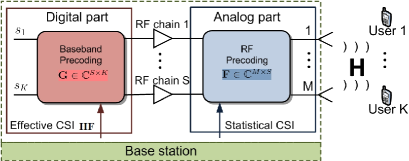
Figure 1: Massive MIMO downlink with THP

Consider a multi-user massive MIMO downlink system with one BS serving $K$ single-antenna users, as illustrated in Fig. 1. For clarity, we focus on a narrowband system with flat block fading channel, but the proposed algorithm can be easily modified to cover the wideband system as well. The BS is equipped with $M$ antennas and $S$ transmit RF chains, where $K\leq S\ll M$. Hybrid precoding is employed to support simultaneous transmissions to the $K$ users with limited RF chains at the BS. In this case, the transmit signal vector for user $k$ is given by $\boldsymbol{F}\boldsymbol{g}_{k}s_{k},$ where $\boldsymbol{F}\in\mathbb{C}^{M\times S}$ is the RF precoder, and $\boldsymbol{g}_{k}\in\mathbb{C}^{S\times 1}$ and $s_{k}\sim\mathcal{CN}\left(0,1\right)$ are the baseband precoding vector and the data symbol for user $k$, respectively. The RF precoder $\boldsymbol{F}$ is usually implemented using an RF phase shifting network [11]. Hence, all elements of $\boldsymbol{F}$ have equal magnitude, i.e., $\left[\boldsymbol{F}\right]_{i,j}=\frac{1}{\sqrt{M}}e^{\sqrt{-1}\theta_{i,j}}$, where $\theta_{i,j}$ is the phase of the $\left(i,j\right)$-th element of $\boldsymbol{F}$. Under hybrid precoding, the received signal for user $k$ is given by

$$y_{k}=\sqrt{p_{k}}\boldsymbol{h}_{k}^{H}\boldsymbol{F}\boldsymbol{g}_{k}s_{k}+\boldsymbol{h}_{k}^{H}\sum_{i\neq k}\sqrt{p_{i}}\boldsymbol{F}\boldsymbol{g}_{i}s_{i}+z_{k},$$ (1)

where $\boldsymbol{h}_{k}\in\mathbb{C}^{M}$ is the channel of user $k$, $p_{k}$ is the transmit power allocated to user $k$, and $z_{k}\sim\mathcal{CN}\left(0,1\right)$ is the additive white Gaussian noise (AWGN).

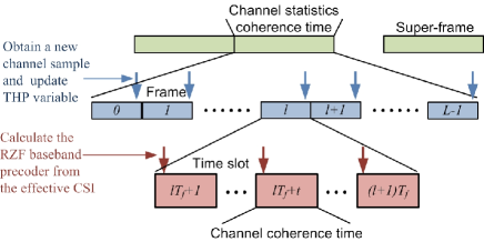
Figure 2: Timeline (frame structure) of SSCA-THP algorithm

In this paper, we consider a THP scheme, whose time line is illustrated in Fig. 2. The time domain is divided into super-frames. Each super-frame is further divided into $L$ frames, and each frame consists of $T_{f}$ time slots. The channel statistics (distribution) are assumed to be constant within each super-frame, and the channel state $\boldsymbol{H}$ is assumed to be constant within each time slot. We assume that the BS can obtain the real-time effective CSI $\boldsymbol{H}\boldsymbol{F}$ at each time slot, and one (possibly outdated) channel sample $\boldsymbol{H}$ at each frame. In our design, the BS is not required to have explicit knowledge of the channel statistics. By observing one channel sample at each frame, the proposed algorithm can automatically learn the channel statistics (in an implicit way). Specifically, the RF precoder $\mathbf{F}$ is only updated once per frame based on the (possibly outdated) channel sample to achieve massive MIMO array gain with reduced implementation cost. On the other hand, the baseband precoder $\boldsymbol{G}=\left[\boldsymbol{g}_{1},...,\boldsymbol{g}_{K}\right]$ is adaptive to the real-time effective CSI $\boldsymbol{H}\boldsymbol{F}\in\mathbb{C}^{K\times S}$ to achieve the spatial multiplexing gain, where $\boldsymbol{H}=\left[\boldsymbol{h}_{1},...,\boldsymbol{h}_{K}\right]^{H}\in\mathbb{C}^{K\times M}$ is the composite downlink channel. We consider a regularized zero-forcing (RZF) baseband precoder [12]:

$$\boldsymbol{G}=\boldsymbol{F}^{H}\boldsymbol{H}^{H}\left(\boldsymbol{H}\boldsymbol{F}\boldsymbol{F}^{H}\boldsymbol{H}^{H}+\alpha\boldsymbol{I}\right)^{-1}\boldsymbol{\Lambda}^{1/2},$$ (2)

where $\alpha$ is the regularization factor, $\boldsymbol{\Lambda}=\textrm{Diag}\left(\left[\left\|\overline{\boldsymbol{g}}_{1}\right\|^{-1},...,\left\|\overline{\boldsymbol{g}}_{K}\right\|^{-1}\right]\right)$ is used to normalize the precoding vectors $\boldsymbol{F}\boldsymbol{g}_{k}$’s, and $\overline{\boldsymbol{g}}_{k}$ is the $k$-th column of $\overline{\boldsymbol{G}}\triangleq\boldsymbol{F}\boldsymbol{F}^{H}\boldsymbol{H}^{H}\left(\boldsymbol{H}\boldsymbol{F}\boldsymbol{F}^{H}\boldsymbol{H}^{H}+\alpha\boldsymbol{I}\right)^{-1}$.

Although the baseband precoder $\boldsymbol{G}$ is adaptive to the instantaneous effective CSI, as in (2), we assume that the regularization factor $\alpha$ and the power allocation $\boldsymbol{p}=\left[p_{1},...,p_{K}\right]^{T}$ are adaptive to the channel statistics only. This is because in the massive MIMO regime, the system tends to behave like a deterministic system and thus the gain of adapting the power allocation and regularization factor according to the instantaneous CSI is small [13, 14]. Similar assumptions have also been made in [15, 6, 5] to achieve a good compromise between performance and complexity.

II-B Various Implementation Methods for RF Precoder

Various implementation methods for the RF precoder $\boldsymbol{F}$ have been proposed in the literature to achieve different tradeoffs between the performance, complexity and power consumption. Basically, there are two major RF precoding structures: the fully-connected structure and the partially-connected structure. For each structure, there are two common methods to dynamically adjust the RF precoder. In this subsection, we shall discuss the existing typical implementations for the RF precoder and their pros and cons.

One major challenge for the optimization of the RF precoder is that it has a discrete implementation constraint; e.g., the phase shifter cannot take a continuous value in practice and has to be quantized into discrete values. In this subsection, we will also discuss two techniques to convert the discrete RF precoder into continuous variables to make the optimization of the RF precoder tractable.

II-B1 Fully-connected RF Precoding Structure

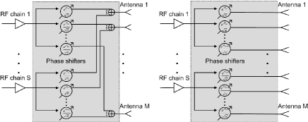
Figure 3: Fully-connected and partially-connected structures in RF precoder

In this case, each RF chain is connected to every antenna through phase shifters and RF adders. To be more specific, if a BS has $M$ antennas and $S$ RF chains, $MS$ phase shifters and $M$ RF adders will be required to implement the RF precoder, as illustrated in Fig. 3-(a). There are two methods to dynamically adjust the RF precoder, as elaborated below.

DPS-based RF Precoder: In this method, each phase shifter is quantized using $B$ bits. Then each phase shifter $\theta_{i,j}$ can take a value from the discrete set $\left\{0,\frac{2\pi}{2^{B}},...,\frac{2\pi\left(2^{B}-1\right)}{2^{B}}\right\}$. Since the phase of each element of the RF precoder can be quantized and adjusted individually, the DPS-based RF precoder can achieve a good performance. However, the requirement of a large number of dynamic phase shifters and RF adders increases the hardware cost and power consumption.

The DPS-based RF precoder can be represented by a phase vector $\boldsymbol{\theta}\in\mathbb{R}^{MS}$ whose $\left(\left(j-1\right)M+i\right)$-th element is $\theta_{i,j}$, and the optimization of the DPS-based RF precoder is a discrete optimization problem due to the discrete constraint on $\theta_{i,j}$. To make the problem tractable, we first ignore the discrete constraint and treat $\theta_{i,j}$ as a continuous variable. After finding the optimized phase vector $\boldsymbol{\theta}^{*}$, we project it onto the feasible set to obtain the final phase vector $\hat{\boldsymbol{\theta}}$:

$$\hat{\theta}_{i,j} =\underset{\theta\in\left\{0,...,2\pi\left(2^{B}-1\right)/2^{B}\right\}}{\text{argmin}}\left|\left(\theta_{i,j}^{*}\textrm{ mod }2\pi\right)-\theta\right|,$$ (3)

$\forall i,j$, where mod denotes the modulo operation. With only $B=3$ bits, the performance loss due to the quantization effect is already small [16].

Codebook-based RF Precoder: In this case, each column of the RF precoder can only be selected from a finite-size codebook $\mathcal{F}=\left\{\boldsymbol{c}_{1},...,\boldsymbol{c}_{N}\right\}$ with $\left|\mathcal{F}\right|=N$ code vectors. The RF precoding codebook $\mathcal{F}$ is usually chosen to be the array response vectors at the BS. For example, when a uniform linear array (ULA) is used, the array response vectors form a DFT matrix. The codebook-based RF precoder can be easily implemented using a static precoder at the RF domain (using a static phase shifting network) together with an RF switch [6]. However, the performance of the codebook-based RF precoder is in general worse than that of the DPS-based RF precoder.

The codebook-based RF precoder can be represented by a selection matrix as $\boldsymbol{F}=\boldsymbol{C}\boldsymbol{D}$, where $\boldsymbol{C}=\left[\boldsymbol{c}_{1},...,\boldsymbol{c}_{N}\right]\in\mathbb{C}^{M\times N}$ is the codebook matrix, and $\boldsymbol{D}\triangleq\textrm{Diag}\left(\boldsymbol{d}\right)$ with $\boldsymbol{d}=\left[d_{1},...,d_{N}\right]^{T}\in\left\{0,1\right\}^{N}$ and $\sum_{i=1}^{N}d_{i}=S$ is a selection matrix. The optimization of the codebook-based RF precoder is an integer optimization problem due to the constraint $d_{i}\in\left\{0,1\right\},\forall i=1,...,N$. Note that the constraints $\sum_{i=1}^{N}d_{i}=S$ and $d_{i}\in\left\{0,1\right\},\forall i$ are equivalent to the following constraints:

$$\sum_{i=1}^{N}d_{i}=S,\>d_{i}\in\left[0,1\right],\>\left\|\boldsymbol{d}\right\|_{0}\leq S.$$ (4)

To make the problem tractable, we approximate the $l_{0}$-norm $\left\|\boldsymbol{d}\right\|_{0}$ using a smooth function as [17]

$$\left\|\boldsymbol{d}\right\|_{0}\approx\sum_{i=1}^{N}\log\left(1+\frac{d_{i}}{\epsilon}\right)/\log\left(1+\frac{1}{\epsilon}\right),\>\boldsymbol{d}\in\left[0,1\right]^{N},$$ (5)

where the smooth parameter $\epsilon>0$ can be used to control the approximation error. A smaller $\epsilon$ leads to smaller approximation error but a less smooth function. Then we can replace the constraint $\left\|\boldsymbol{d}\right\|_{0}\leq S$ with a non-convex sparse constraint

$$\sum_{i=1}^{N}\log\left(1+\frac{d_{i}}{\epsilon}\right)/\log\left(1+\frac{1}{\epsilon}\right)\leq S,$$ (6)

which can be handled using the SSCA-THP algorithm. Note that the sparse constraint (6) has been widely used in compressive sensing to impose sparsity on sparse signals [17]. After finding the optimized selection vector $\boldsymbol{d}^{*}$, we project it onto the feasible set to obtain the final solution $\hat{\boldsymbol{d}}$:

$$\hat{\boldsymbol{d}}=\underset{\boldsymbol{d}}{\textrm{argmin}}\left\|\boldsymbol{d}-\boldsymbol{d}^{*}\right\|,\textrm{ s.t.}\>\boldsymbol{d}\in\left\{0,1\right\}^{N},\left\|\boldsymbol{d}\right\|_{0}=S.$$

Specifically, $\hat{\boldsymbol{d}}$ is a binary vector whose $S$ non-zero elements are located at the $S$ largest elements of $\boldsymbol{d}^{*}$. Thanks to the sparse constraint on $\boldsymbol{d}^{*}$, $\boldsymbol{d}^{*}$ is usually close to a binary vector with $S$ non-zero elements, and thus the performance loss due to the above projection is very small.

II-B2 Partially-connected RF Precoding Structure

In this case, each RF chain is connected to a sub-array of antennas via phase shifters and each antenna is only connected to a single RF chain [9], as illustrated in Fig. 3-(b). Such a partially-connected structure presents a block diagonal form as $\boldsymbol{F}=\textrm{BlockDiag}\left(\boldsymbol{f}_{1},\boldsymbol{f}_{2},...,\boldsymbol{f}_{S}\right)$, where $\boldsymbol{f}_{s}\in\mathbb{C}^{M/S}$ is the $s$-th precoding vector corresponding to the $s$-th RF chain. Note that we have assumed that $M$ is divisible by $S$ for easy illustration. The partially-connected structure only requires a total number of $M$ phase shifters (instead of $MS$ phase shifters in the fully-connected case). As a result, it has much lower power consumption and hardware complexity compared to the fully-connected case. However, the performance of the partially-connected RF precoder is compromised.

The DPS-based or codebook-based method can be used to adjust the partially-connected RF precoder. In the DPS-based method, the partially-connected RF precoder can be represented by a phase vector $\boldsymbol{\theta}\in\mathbb{R}^{M}$ whose $\left(\left(j-1\right)M/S+i\right)$-th element is $\theta_{i,j}$ for $i=\left(j-1\right)M/S+1,...,jM/S$; $j=1,...,S$. Similarly, to make the problem tractable, we first ignore the discrete constraint on $\theta_{i,j}$ and then project the resulting solution onto the discrete set using (3).

In the codebook-based method, the $s$-th RF precoding vector $\boldsymbol{f}_{s}$ is selected from a finite-size codebook $\mathcal{F}_{s}=\left\{\mathbf{c}_{1},...,\mathbf{c}_{N}\right\}$ with $\left|\mathcal{F}_{s}\right|=N$ code vectors. Let $\boldsymbol{C}_{s}=\left[\boldsymbol{c}_{s,1},...,\boldsymbol{c}_{s,N}\right]\in\mathbb{C}^{\frac{M}{S}\times N}$ denote the codebook matrix for $\boldsymbol{f}_{s}$. Then the $s$-th RF precoding vector $\boldsymbol{f}_{s}$ can be represented as $\boldsymbol{f}_{s}=\boldsymbol{C}_{s}\boldsymbol{D}_{s}$, where $\boldsymbol{D}_{s}\triangleq\textrm{Diag}\left(\boldsymbol{d}_{s}\right)$ with $\boldsymbol{d}_{s}=\left[d_{s,1},...,d_{s,N}\right]^{T}\in\left\{0,1\right\}^{N}$ and $\sum_{i=1}^{N}d_{s,i}=1$ is a selection matrix. For convenience, let $\boldsymbol{d}=\left[\boldsymbol{d}_{1},...,\boldsymbol{d}_{S}\right]$ denote the overall selection vector. Similarly, we can use the “sparse” technique to relax the integer constraints $d_{s,i}\in\left\{0,1\right\},\forall s,i$ to non-convex smooth constraints $\sum_{i=1}^{N}d_{s,i}=1,\>d_{s,i}\in\left[0,1\right],\>\sum_{i=1}^{N}\log\left(1+\frac{d_{s,i}}{\epsilon}\right)/\log\left(1+\frac{1}{\epsilon}\right)\leq 1.$

II-C Achievable Data Rate

Under different implementation methods, the RF precoder $\boldsymbol{F}$ is represented by different parameters with different dimensions. For convenience, we use $\boldsymbol{\phi}$ as a unified notation to denote the RF precoding parameter. For example, in the DPS-based method, $\boldsymbol{\phi}=\boldsymbol{\theta}$ and its dimension is $MS$ and $M$ for the fully-connected and partially-connected structures, respectively. In the codebook-based method, $\boldsymbol{\phi}=\boldsymbol{d}$ and its dimension is $N$ and $NS$ for the fully-connected and partially-connected structures, respectively.

For given RF precoding parameter $\boldsymbol{\phi},$ power allocation $\boldsymbol{p}$, the RZF regularization factor $\alpha$ in (2) and channel realization $\boldsymbol{H}$, the instantaneous achievable data rate of user $k$ is

$$r_{k}\left(\boldsymbol{\phi},\boldsymbol{p},\alpha;\boldsymbol{H}\right)=\log\left(1+\frac{p_{k}\left|\boldsymbol{h}_{k}^{H}\boldsymbol{F}\boldsymbol{g}_{k}\right|^{2}}{\sum_{i\neq k}p_{i}\left|\boldsymbol{h}_{k}^{H}\boldsymbol{F}\boldsymbol{g}_{i}\right|^{2}+1}\right).$$

Note that $\boldsymbol{F}$ is a function of $\boldsymbol{\phi}$ and $\boldsymbol{G}$ is a function of $\boldsymbol{\phi},\boldsymbol{p},\alpha$ and $\boldsymbol{H}$. Therefore, we explicitly express $r_{k}$ as a function of $\boldsymbol{\phi},\boldsymbol{p},\alpha$ which depends on the random channel state $\boldsymbol{H}$. The average data rate of user $k$ is

$$\overline{r}_{k}\left(\boldsymbol{\phi},\boldsymbol{p},\alpha\right)=\mathbb{E}\left[r_{k}\left(\boldsymbol{\phi},\boldsymbol{p},\alpha;\boldsymbol{H}\right)\right].$$

For convenience, define $\overline{\boldsymbol{r}}\left(\boldsymbol{\phi},\boldsymbol{p},\alpha\right)\triangleq[\overline{r}_{1}\left(\boldsymbol{\phi},\boldsymbol{p},\alpha\right),...,\overline{r}_{K}\left(\boldsymbol{\phi},\boldsymbol{p},\alpha\right)]^{T}$ as the average data rate vector.

II-D THP Optimization Formulation

Consider the following general optimization formulation for the design of THP:

$$\min_{\boldsymbol{x}\in\mathcal{X}}\>f_{0}\left(\boldsymbol{x}\right)\triangleq h_{0}\left(\overline{\boldsymbol{r}}\left(\boldsymbol{\phi},\boldsymbol{p},\alpha\right),\boldsymbol{x}\right)$$ (7)

s.t. $$f_{i}\left(\boldsymbol{x}\right)\triangleq h_{i}\left(\overline{\boldsymbol{r}}\left(\boldsymbol{\phi},\boldsymbol{p},\alpha\right),\boldsymbol{x}\right)\leq 0,i=1,....,m,$$

where $\boldsymbol{x}=\left[\boldsymbol{\phi}^{T},\boldsymbol{p}^{T},\alpha,\boldsymbol{\beta}^{T}\right]^{T}$ is called the THP variable, $\boldsymbol{\beta}\in\mathbb{R}^{n_{\beta}}$, with dimension $n_{\beta}$, is an additional optimization variable that does not affect the average data rate vector $\overline{\boldsymbol{r}}$, and $\mathcal{X}\subseteq\mathbb{R}^{n}$ is a convex set. The motivation for introducing an additional optimization variable $\boldsymbol{\beta}$ is to provide extra flexibility in the formulation to cover more application scenarios, as will be shown in Example 4 at the end of this subsection. Note that both the dimension $n$ and the set $\mathcal{X}$ depend on the implementation method for the RF precoder. For example, for the codebook-based RF precoder, we have

$$\mathcal{X}=\left\{\boldsymbol{x}:\boldsymbol{d}\in\left[0,1\right]^{N};\boldsymbol{p}\in\left[0,\tilde{p}\right]^{K};\alpha>\tilde{\alpha};\boldsymbol{\beta}\in\mathcal{B}\right\},$$ (8)

where $\tilde{p}>0$ is used to ensure that the transmit power is bounded, $\tilde{\alpha}>0$ is a small number to ensure that the calculation of the matrix inverse in (2) is always numerically stable, $\mathcal{B}=\left\{\boldsymbol{\beta}:\>\beta_{i}\in\mathcal{B}_{i},i=1,...,n_{\beta}\right\}$, and $\mathcal{B}_{i}$ is a convex region in $\mathbb{R}$. Note that, without loss of generality, all the coupled constraints on $\boldsymbol{x}$, such as the sparse constraint (6) on the codebook-based RF precoding parameter $\boldsymbol{d}$, are included in the explicit constraints $f_{i}\left(\boldsymbol{x}\right)\leq 0,i=1,....,m$. As a result, $\mathcal{X}$ has a decoupled form: $\mathcal{X}=\left\{\boldsymbol{x}:\>x_{i}\in\mathcal{X}_{i},i=1,...,n\right\}$, where $\mathcal{X}_{i}$ is a convex region in $\mathbb{R}$. We assume that the functions $h_{i}\left(\overline{\boldsymbol{r}},\boldsymbol{x}\right),i=0,...,m$ are continuously differentiable (and possibly non-convex) functions of $\left(\overline{\boldsymbol{r}},\boldsymbol{x}\right)$.

Problem (7) embraces many applications as special cases. In the following, we give some important examples.

Example 1 (Sum throughput maximization [4]).

The sum throughput maximization problem is formulated as:

$$\max_{\boldsymbol{x}\in\mathcal{X}}\>\sum_{k=1}^{K}\overline{r}_{k}\left(\boldsymbol{\phi},\boldsymbol{p},\alpha\right),\textrm{ s.t. }\sum_{k=1}^{K}p_{k}\leq P,$$ (9)

where $P$ is the total power constraint at the BS. This is an instance of Problem (7) with $h_{0}\left(\overline{\boldsymbol{r}},\boldsymbol{x}\right)=-\sum_{k=1}^{K}\overline{r}_{k}$, $h_{1}\left(\overline{\boldsymbol{r}},\boldsymbol{x}\right)=\sum_{k=1}^{K}p_{k}-P$ and $\mathcal{B}=\emptyset$ (i.e., there is no additional variable $\boldsymbol{\beta}$).

Example 2 (PFS [18]).

PFS is a widely used utility function in wireless resource optimization. The PFS utility maximization problem is formulated as:

$$\max_{\boldsymbol{x}\in\mathcal{X}}\>\sum_{k=1}^{K}\textrm{log}\left(\varepsilon+\overline{r}_{k}\left(\boldsymbol{\phi},\boldsymbol{p},\alpha\right)\right),\textrm{ s.t. }\sum_{k=1}^{K}p_{k}\leq P,$$ (10)

where $\varepsilon>0$ is a small number used to avoid the singularity at $\overline{r}_{k}=0$ [19]. This is an instance of Problem (7) with $h_{0}\left(\overline{\boldsymbol{r}},\boldsymbol{x}\right)=-\sum_{k=1}^{K}\textrm{log}\left(\varepsilon+\overline{r}_{k}\right)$, $h_{1}\left(\overline{\boldsymbol{r}},\boldsymbol{x}\right)=\sum_{k=1}^{K}p_{k}-P$ and $\mathcal{B}=\emptyset$.

Example 3 (Power minimization with individual QoS requirements [20]).

In this example, the THP variable $\boldsymbol{x}$ is designed to minimize the average transmit power subject to individual QoS requirements as follows:

$$\min_{\boldsymbol{x}\in\mathcal{X}}\>\sum_{k=1}^{K}p_{k},\textrm{ s.t. }\overline{r}_{k}\left(\boldsymbol{\phi},\boldsymbol{p},\alpha\right)\geq\gamma_{k},\forall k,$$ (11)

where each user has an individual QoS requirement in terms of the average data rate constraint $\overline{r}_{k}\left(\boldsymbol{\phi},\boldsymbol{p},\alpha\right)\geq\gamma_{k}$, and the constant $\gamma_{k}\geq 0$ is the target rate for user $k$. This is an instance of Problem (7) with $h_{0}\left(\overline{\boldsymbol{r}},\boldsymbol{x}\right)=\sum_{k=1}^{K}p_{k}$, $h_{k}\left(\overline{\boldsymbol{r}},\boldsymbol{x}\right)=\gamma_{k}-\overline{r}_{k},\forall k$ and $\mathcal{B}=\emptyset$.

Example 4 (MWTM [6]).

In this example, the THP variable $\boldsymbol{x}$ is designed to maximize the minimum (weighted) average data rate of users as follows:

$$\max_{\boldsymbol{x}\in\mathcal{X}}\>\min_{k}\frac{1}{w_{k}}\overline{r}_{k}\left(\boldsymbol{\phi},\boldsymbol{p},\alpha\right),\textrm{ s.t. }\sum_{k=1}^{K}p_{k}\leq P,$$ (12)

where $w_{k}>0$ is the weight for user $k$, which can be used to provide a differential QoS for different users. (12) is not an instance of Problem (7) because the objective function is non-smooth. However, by introducing an auxiliary variable $\beta$, we can convert (12) to an instance of Problem (7) as:

$$\max_{\boldsymbol{x}\in\mathcal{X}}\>\beta,\textrm{ s.t. }\overline{r}_{k}\left(\boldsymbol{\phi},\boldsymbol{p},\alpha\right)\geq w_{k}\beta,\forall k;\sum_{k=1}^{K}p_{k}\leq P,$$ (13)

with $h_{0}\left(\overline{\boldsymbol{r}},\boldsymbol{x}\right)=-\beta$, $h_{k}\left(\overline{\boldsymbol{r}},\boldsymbol{x}\right)=w_{k}\beta-\overline{r}_{k},\forall k$, $h_{K+1}\left(\overline{\boldsymbol{r}},\boldsymbol{x}\right)=\sum_{k=1}^{K}p_{k}-P$ and $\mathcal{B}=\left\{\beta:\>\beta\geq 0\right\}$.

There are several challenges to solve Problem (7). First, the average data rates $\overline{r}_{k}\left(\boldsymbol{\phi},\boldsymbol{p},\alpha\right)$’s are neither convex nor concave, and have no closed-form expressions. Moreover, the presence of stochastic non-convex constraints further complicates Problem (7). In the next section, we shall propose an efficient algorithm based on the SSCA method, called SSCA-THP, to find a stationary point of Problem (7).

III Stochastic Successive Convex Approximation for THP Optimization

III-A The SSCA-THP Algorithm

At each iteration, the THP variable $\boldsymbol{x}$ is updated by solving a quadratic optimization problem obtained by replacing the objective and constraint functions $f_{i}\left(\boldsymbol{x}\right),i=0,...,m$ with their quadratic surrogate functions $\bar{f}_{i}^{l}\left(\boldsymbol{x}\right),i=0,...,m$.

Algorithm 1 summarizes the key steps of the proposed SSCA-THP algorithm. Specifically, at iteration $l$, a new realization of the random channel state $\boldsymbol{H}^{l}$ is obtained in Step 1 and the surrogate functions $\bar{f}_{i}^{l}\left(\boldsymbol{x}\right),\forall i$ are updated based on $\boldsymbol{H}^{l}$ and the current iterate $\boldsymbol{x}^{l}$ as

$$\bar{f}_{i}^{l}\left(\boldsymbol{x}\right) =h_{i}\left(\hat{\boldsymbol{r}}^{l},\boldsymbol{x}^{l}\right)+\left(\mathbf{u}_{i}^{l}\right)^{T}\left(\boldsymbol{x}-\boldsymbol{x}^{l}\right)+\tau_{i}\left\|\boldsymbol{x}-\boldsymbol{x}^{l}\right\|^{2},$$ (14)

where $\tau_{i}>0$ is a constant; $\hat{\boldsymbol{r}}^{l}=\left[\hat{r}_{1}^{l},...,\hat{r}_{K}^{l}\right]^{T}$, with $\hat{r}_{k}^{l}=\sum_{j=1}^{l}r_{k}\left(\boldsymbol{\phi}^{l},\boldsymbol{p}^{l},\alpha^{l};\boldsymbol{H}^{j}\right)/l$, is the sample average approximations for $\overline{r}_{k}\left(\boldsymbol{\phi}^{l},\boldsymbol{p}^{l},\alpha^{l}\right)$; $\mathbf{u}_{i}^{l}$ is an approximation for the gradient $\nabla f_{i}\left(\boldsymbol{x}^{l}\right)$, which is updated recursively as

$$\mathbf{u}_{i}^{l} =\left(1-\rho^{l}\right)\mathbf{u}_{i}^{l-1}+\rho^{l}\hat{\mathbf{u}}_{i}^{l},$$

with $\mathbf{u}^{-1}=\boldsymbol{0}$, where $\rho^{l}\in\left(0,1\right]$ is a sequence to be properly chosen and

$$\hat{\mathbf{u}}_{i}^{l} =\mathbf{J}_{r}\left(\boldsymbol{x}^{l};\boldsymbol{H}^{l}\right)\nabla_{\overline{\boldsymbol{r}}}h_{i}\left(\hat{\boldsymbol{r}}^{l},\boldsymbol{x}^{l}\right)+\nabla_{\boldsymbol{x}}h_{i}\left(\hat{\boldsymbol{r}}^{l},\boldsymbol{x}^{l}\right),$$ (15)

where $\mathbf{J}_{r}\left(\boldsymbol{x}^{l};\boldsymbol{H}^{l}\right)$ is the Jacobian matrix of the instantaneous rate vector $\boldsymbol{r}\left(\boldsymbol{\phi},\boldsymbol{p},\alpha;\boldsymbol{H}\right)\triangleq[r_{1}\left(\boldsymbol{\phi},\boldsymbol{p},\alpha;\boldsymbol{H}\right),...,r_{K}\left(\boldsymbol{\phi},\boldsymbol{p},\alpha;\boldsymbol{H}\right)]^{T}$ and its expression is derived in Appendix -A, $\nabla_{\overline{\boldsymbol{r}}}h_{i}$ and $\nabla_{\boldsymbol{x}}h_{i}$ are the gradients of $h_{i}$ w.r.t. the average rate vector $\overline{\boldsymbol{r}}$ and the THP variable $\boldsymbol{x}$, respectively. The surrogate function $\bar{f}_{i}^{l}\left(\boldsymbol{x}\right)$ can be viewed as a convex approximation of $f_{i}\left(\boldsymbol{x}\right)$ in a local domain around $\boldsymbol{x}^{l}$.

In Step 2, the optimal solution $\bar{\boldsymbol{x}}^{l}$ of the following problem is solved:

$$\bar{\boldsymbol{x}}^{l}=\underset{\boldsymbol{x}\in\mathcal{X}}{\text{argmin}}\> \bar{f}_{0}^{l}\left(\boldsymbol{x}\right)$$ (16)

$$s.t.\> \bar{f}_{i}^{l}\left(\boldsymbol{x}\right)\leq 0,i=1,....,m,$$

which is a convex approximation of (7). Note that Problem (16) is not necessarily feasible. If Problem (16) turns out to be infeasible, the optimal solution $\bar{\boldsymbol{x}}^{l}$ of the following convex problem is solved:

$$\bar{\boldsymbol{x}}^{l}=\underset{\boldsymbol{x}\in\mathcal{X},\nu}{\text{argmin}} \>\nu$$ (17)

$$s.t.\> \bar{f}_{i}^{l}\left(\boldsymbol{x}\right)\leq\nu,i=1,....,m,$$

which minimizes the constraint functions.

Given $\bar{\boldsymbol{x}}^{l}$ in one of the above two cases, $\boldsymbol{x}$ is updated in Step 3 according to

$$\boldsymbol{x}^{l+1}=\left(1-\gamma^{l}\right)\boldsymbol{x}^{l}+\gamma^{l}\bar{\boldsymbol{x}}^{l},$$ (18)

where $\gamma^{l}\in\left(0,1\right]$ is a sequence to be properly chosen. Then the above iteration (Steps 1 to 3) is carried out until convergence.

Algorithm 1 SSCA-THP Algorithm

Input: $\left\{\gamma^{l}\right\}$, $\left\{\rho^{l}\right\}$.

Initialize: $\boldsymbol{x}^{0}\in\mathcal{X}$; $\mathbf{u}_{i}^{-1}=\boldsymbol{0},\forall i$, $l=0$.

Step 1: Obtain a channel sample $\boldsymbol{H}^{l}$ within frame $l$.

Update the surrogate functions $\bar{f}_{i}^{l}\left(\boldsymbol{x}\right),\forall i$ using (14).

Step 2: Solve (17) to obtain the optimal solution $\nu^{\circ},\boldsymbol{x}^{\circ}$.

If $\nu^{\circ}\leq 0$ (Problem (16) is feasible)

Solve (16) to obtain $\bar{\boldsymbol{x}}^{l}$. //Objective update

Else

Let $\bar{\boldsymbol{x}}^{l}=\boldsymbol{x}^{\circ}$. //Feasible update

End if

Step 3: Update $\boldsymbol{x}^{l+1}$ according to (18).

Step 4: Let $l=l+1$ and return to Step 1.

III-B Efficient Solutions for Quadratic Optimization Subproblems

In this subsection, we propose efficient solutions for the quadratic optimization subproblems in (16) and (17) based on the Lagrange dual method. The reasons for using the Lagrange dual method are as follows. First, for given Lagrange multipliers (which are also called dual variables), the problem of minimizing the Lagrange function has a unique and closed-form solution. Second, the number of primal variables $\boldsymbol{x}$ is usually much larger than the number of constraints (dual variables) in the massive MIMO regime. Therefore, the optimal dual variables can be solved much more efficiently than directly solving the optimal primal variables.

In the following, we show how to use the Lagrange dual method to solve the subproblem in (16). Since both subproblems have the same form (i.e., both are strictly convex and quadratic optimization problems), the solution for (17) is similar and is omitted for conciseness.

The Lagrange function for (16) is

$$\mathcal{L}^{l}\left(\boldsymbol{x},\boldsymbol{\lambda}\right) =\bar{f}_{0}^{l}\left(\boldsymbol{x}\right)+\sum_{i=1}^{m}\lambda_{i}\bar{f}_{i}^{l}\left(\boldsymbol{x}\right)$$

$$=\sum_{i=1}^{n}a\left(\boldsymbol{\lambda}\right)x_{i}^{2}+b_{i}\left(\boldsymbol{\lambda}\right)x_{i}+c\left(\boldsymbol{\lambda}\right),\>\boldsymbol{x}\in\mathcal{X},$$

where $\boldsymbol{\lambda}=\left[\lambda_{1},...,\lambda_{m}\right]^{T}\in\mathbb{R}_{+}^{m}$ are the Lagrange multipliers,

$$a\left(\boldsymbol{\lambda}\right) =\sum_{j=0}^{m}\lambda_{j}\tau_{j},$$

$$b_{i}\left(\boldsymbol{\lambda}\right) =\sum_{j=0}^{m}\lambda_{j}\left(u_{j,i}^{l}-2\tau_{j}x_{i}^{l}\right),$$

$$c\left(\boldsymbol{\lambda}\right) =\sum_{j=0}^{m}\lambda_{j}\left(h_{j}\left(\hat{\boldsymbol{r}}^{l},\boldsymbol{x}^{l}\right)-\left(\mathbf{u}_{j}^{l}\right)^{T}\boldsymbol{x}^{l}+\tau_{j}\left\|\boldsymbol{x}^{l}\right\|^{2}\right),$$

$\lambda_{0}=1$, and $x_{i}^{l}$ and $u_{j,i}^{l}$ are the $i$-th element of $\boldsymbol{x}^{l}$ and $\mathbf{u}_{j}^{l}$, respectively. The dual function for (16) is

$$g^{l}\left(\boldsymbol{\lambda}\right)=\min_{\boldsymbol{x}\in\mathcal{X}}\mathcal{L}^{l}\left(\boldsymbol{x},\boldsymbol{\lambda}\right).$$ (19)

And the corresponding dual problem is

$$\max_{\boldsymbol{\lambda}\geq\boldsymbol{0}}\>g^{l}\left(\boldsymbol{\lambda}\right).$$ (20)

The minimization problem in (19) can be decomposed into $n$ independent subproblems as

$$\min_{x_{i}\in\mathcal{X}_{i}}a\left(\boldsymbol{\lambda}\right)x_{i}^{2}+b_{i}\left(\boldsymbol{\lambda}\right)x_{i},\>i=1,...,n,$$

which have the following closed-form solutions:

$$x_{i}^{\circ}\left(\boldsymbol{\lambda}\right)=\mathbb{P}_{\mathcal{X}_{i}}\left[-\frac{b_{i}\left(\boldsymbol{\lambda}\right)}{2a\left(\boldsymbol{\lambda}\right)}\right],\forall i,$$ (21)

where $\mathbb{P}_{\mathcal{X}_{i}}\left[\cdot\right]$ denotes the one-dimensional projection on to the convex set $\mathcal{X}_{i}$. On the other hand, the dual function $g\left(\boldsymbol{\lambda}\right)$ is concave and it can be verified that $\left[\bar{f}_{1}^{l}\left(\boldsymbol{x}^{\circ}\left(\boldsymbol{\lambda}\right)\right),,...,\bar{f}_{m}^{l}\left(\boldsymbol{x}^{\circ}\left(\boldsymbol{\lambda}\right)\right)\right]^{T}$ is a subgradient of $g\left(\boldsymbol{\lambda}\right)$ at $\boldsymbol{\lambda}$. Hence, the standard subgradient-based methods such as the subgradient algorithm in [21] or the ellipsoid method in [22] can be used to solve the optimal solution $\boldsymbol{\lambda}^{\circ}$ of the dual problem in (20). Then the optimal primal solution of (16) is given by $\boldsymbol{x}^{\circ}\left(\boldsymbol{\lambda}^{\circ}\right)$.

III-C Implementation Consideration

At the beginning of each super-frame, the BS resets the SSCA-THP algorithm with an initial THP variable $\boldsymbol{x}^{0}$. Then the THP variable $\boldsymbol{x}$ is updated once every frame. Therefore, each frame corresponds to an iteration in the SSCA-THP algorithm. Specifically, let $\boldsymbol{x}^{l}=\left[\left(\boldsymbol{\phi}^{l}\right)^{T},\left(\boldsymbol{p}^{l}\right)^{T},\alpha^{l},\left(\boldsymbol{\beta}^{l}\right)^{T}\right]^{T}$ denote the THP variable used during the $l$-th frame. At time slot $t$ in the $l$-th frame, the BS first acquires the effective channel $\boldsymbol{H}\left(t\right)\boldsymbol{F}^{l}$, where $\boldsymbol{H}\left(t\right)$ is the channel state at time slot $t$, and $\boldsymbol{F}^{l}$ is the RF precoder corresponding to $\boldsymbol{\phi}^{l}$. Then it calculates the baseband precoder $\boldsymbol{G}\left(t\right)$ from $\boldsymbol{H}\left(t\right)\boldsymbol{F}^{l}$ and $\boldsymbol{p}^{l},\alpha^{l}$ using (2). At the end of the $l$-th frame, the BS obtains a channel sample $\boldsymbol{H}^{l}$ and updates the THP variable $\boldsymbol{x}$ by solving a simple quadratic optimization problem, where the updated THP variable $\boldsymbol{x}^{l+1}$ will be used in the $\left(l+1\right)$-th frame. Then the same procedure is carried out in the next frame.

Remark 1.

The proposed SSCA-THP algorithm exploits some unique properties of hybrid beamforming massive MIMO systems to improve the performance and reduce the complexity. For example, the optimization variables and constraints in Section II-B are specifically designed for hybrid beamforming with different RF precoding structures. By imposing the sparse constraint in (6), the property of limited RF chains in massive MIMO is also exploited to improve the performance over the existing semidefinite relaxation (SDR) method in [4] for the codebook-based RF precoder. Finally, the structure of the average data rate function $\overline{r}_{k}\left(\boldsymbol{\theta},\boldsymbol{p},\alpha\right)$ w.r.t. the phase vector $\boldsymbol{\theta}$ is exploited to design quadratic surrogate functions which enables low-complexity and fast-convergent algorithm design.

IV Convergence Analysis

In this section, we establish the local convergence of SSCA-THP to a stationary point. There are several challenges in the convergence proof for SSCA-THP. First, we need to show that at every limiting point, all constraints are satisfied, which is non-trivial since SSCA-THP may oscillate between the feasible update and objective update. Moreover, the limiting point is obtained by averaging over all the previous outputs from either feasible updates or objective updates, which makes it difficult to show that the limiting point is a stationary point of the original Problem (7). In this subsection, we will overcome these challenges and establish the convergence of SSCA-THP. To prove the convergence of SSCA-THP, we need to make the following assumptions on the problem structure.

Assumption 1 (Assumptions on Problem (7)).

 

1. $h_{i}\left(\overline{\boldsymbol{r}},\boldsymbol{x}\right),i=0,...,m$ are continuously differentiable functions of $\left(\overline{\boldsymbol{r}},\boldsymbol{x}\right)$.

2. For any $\boldsymbol{x}\in\mathcal{X}$, the functions $h_{i}\left(\overline{\boldsymbol{r}}\left(\boldsymbol{\phi},\boldsymbol{p},\alpha\right),\boldsymbol{x}\right),i=0,...,m$, their derivative, and their second-order derivative w.r.t. $\overline{\boldsymbol{r}}$ and $\boldsymbol{x}$ are uniformly bounded.

3. $\left\|\boldsymbol{H}^{l}\right\|,l=0,1,...$ are uniformly bounded w.p.1.

4. Let $\boldsymbol{x}_{F}^{*}$ be any stationary point of the following feasibility problem:

   $$\min_{\boldsymbol{x}\in\mathcal{X},\nu}\> \nu$$ (22)

   $$s.t.\> f_{i}\left(\boldsymbol{x}\right)\leq\nu,\>\forall i=1,....,m.$$

   We assume that $f_{i}\left(\boldsymbol{x}_{F}^{*}\right)\leq 0,i=1,...,m$.

The first assumption is standard and is satisfied for a large class of problems. In practice, the channel sample is always bounded, and thus the second assumption is satisfied. The third assumption ensures that Problem (7) is feasible. If there is a stationary point $\boldsymbol{x}_{F}^{*}$ which is not feasible, then Algorithm 1 may get stuck at this stationary point $\boldsymbol{x}_{F}^{*}$. Therefore, the third assumption is necessary for the algorithm to converge to a feasible point of the problem.

Besides Assumption 1, the sequence of parameters $\left\{\rho^{t}\right\},\left\{\gamma^{t}\right\}$ needs to satisfy the following conditions.

Assumption 2 (Assumptions on $\left\{\rho^{t}\right\},\left\{\gamma^{t}\right\}$).

 

1. $\rho^{l}\rightarrow 0$, $\sum_{l}\rho^{l}=\infty$, $\sum_{l}\left(\rho^{l}\right)^{2}<\infty$, $\lim_{l\rightarrow\infty}\rho^{l}l^{-1/2}<\infty$.

2. $\gamma^{l}\rightarrow 0$, $\sum_{l}\gamma^{l}=\infty$, $\sum_{l}\left(\gamma^{l}\right)^{2}<\infty$,

3. $\lim_{l\rightarrow\infty}\gamma^{l}/\rho^{l}=0$.

With Assumptions 1 and 2, we can prove two key lemmas that will eventually lead to the final convergence result. The first lemma proves the convergence of surrogate functions.

Lemma 1 (Convergence of surrogate functions).

Suppose Assumptions 1 and 2 are satisfied. Consider a subsequence $\left\{\boldsymbol{x}^{l_{j}}\right\}_{j=1}^{\infty}$ converging to a limiting point $\boldsymbol{x}^{*}$, and define functions

$$\hat{f}_{i}\left(\boldsymbol{x}\right) \triangleq h_{i}\left(\overline{\boldsymbol{r}}\left(\boldsymbol{\phi}^{*},\boldsymbol{p}^{*},\alpha^{*}\right),\boldsymbol{x}^{*}\right)$$

$$+\nabla f_{i}\left(\boldsymbol{x}^{*}\right)\left(\boldsymbol{x}-\boldsymbol{x}^{*}\right)+\tau_{i}\left\|\boldsymbol{x}-\boldsymbol{x}^{*}\right\|^{2},\forall i,$$

which satisfy $\hat{f}_{i}\left(\boldsymbol{x}^{*}\right)=f_{i}\left(\boldsymbol{x}^{*}\right)$ and $\nabla\hat{f}_{i}\left(\boldsymbol{x}^{*}\right)=\nabla f_{i}\left(\boldsymbol{x}^{*}\right),\forall i$. Then, almost surely, we have

$$\lim_{j\rightarrow\infty}\bar{f}_{i}^{l_{j}}\left(\boldsymbol{x}\right) =\hat{f}_{i}\left(\boldsymbol{x}\right),\>\forall\boldsymbol{x}\in\mathcal{X}.$$ (23)

Please refer to Appendix -B for the proof. To state the convergence result, we need to introduce the concept of Slater condition for the converged surrogate functions.

Slater condition for the converged surrogate functions: Given a subsequence $\left\{\boldsymbol{x}^{l_{j}}\right\}_{j=1}^{\infty}$ converging to a limiting point $\boldsymbol{x}^{*}$ and letting $\hat{f}_{i}\left(\boldsymbol{x}\right),\forall i$ be the converged surrogate functions as defined in Lemma 1, we say that the Slater condition is satisfied at $\boldsymbol{x}^{*}$ if there exists $\boldsymbol{x}\in\textrm{int}\mathcal{X}$ such that

$$\hat{f}_{i}\left(\boldsymbol{x}\right)<0,\>\forall i=1,...,m.$$

A similar Slater condition is also assumed in [23] to prove the convergence of a deterministic majorization-minimization (MM) algorithm with non-convex constraints.

Before the introduction of the main convergence theorem, we give the second key lemma.

Lemma 2.

Let $\left\{\boldsymbol{x}^{l}\right\}_{l=1}^{\infty}$ denote the sequence of iterates generated by Algorithm 1. We have

$$\limsup_{l\rightarrow\infty}\max_{i\in\left\{1,...,m\right\}}f_{i}\left(\boldsymbol{x}^{l}\right) \leq 0,\text{ w.p.1.}$$

$$\lim_{l\rightarrow\infty}\left\|\bar{\boldsymbol{x}}^{l}-\boldsymbol{x}^{l}\right\| =0,\text{ w.p.1.}$$

The lemma states that the algorithm will converge to the feasible region, and the gap between $\bar{\boldsymbol{x}}^{l}$ and $\boldsymbol{x}^{l}$ converges to zero, almost surely. Please refer to Appendix -C for the proof.

Theorem 1 (Convergence of Algorithm 1).

Suppose Assumptions 1 and 2 are satisfied. For any subsequence $\left\{\boldsymbol{x}^{l_{j}}\right\}_{j=1}^{\infty}$ converging to a limit point $\boldsymbol{x}^{*}$, if the Slater condition is satisfied at $\boldsymbol{x}^{*}$, then $\boldsymbol{x}^{*}$ is a stationary point of Problem (7) almost surely.

Please refer to Appendix -D for the proof.

V Applications and Numerical Validation

In this section, we shall apply the proposed SSCA-THP to solve the first three example problems described in Section II. As in [5], we adopt a geometry-based channel model with a half-wavelength space ULA for simulations. The channel vector of user $k$ can be expressed as $\boldsymbol{h}_{k}=\sum_{i=1}^{N_{p}}\alpha_{k,i}\boldsymbol{\textrm{a}}\left(\varphi_{k,i}\right)$, where $\boldsymbol{\textrm{a}}\left(\varphi\right)$ is the array response vector, $\varphi_{k,i}$’s are Laplacian distributed with an angle spread $\sigma_{\textrm{AS}}=10$, $\alpha_{k,i}\sim\mathcal{CN}\left(0,\sigma_{k,i}^{2}\right)$, $\sigma_{k,i}^{2}$ are randomly generated from an exponential distribution and normalized such that $\sum_{i=1}^{N_{p}}\sigma_{k,i}^{2}=g_{k}$, and $g_{k}$ represents the path gain of user $k$. Unless otherwise specified, we consider $M=64$ antennas, $S=16$ RF chains and $N_{p}=6$ channel paths. The path gains $g_{k}$’s are uniformly generated between -10 dB and 10 dB. The DPS-based RF precoder is considered in Example 1 and 2, while both the DPS-based and codebook-based RF precoders are considered in Example 3. We compare the performance of the SSCA-THP with the following baseline algorithms.

Baseline 1 (SAA): This is the sample average approximation algorithm. Specifically, after applying SAA, the problem becomes a deterministic non-convex optimization problem, which is then solved using the deterministic successive convex approximation method [23].

Baseline 2 (SLNR-max): This is the SLNR maximization algorithm in [5].

Baseline 3 (JSDM): This is the the joint spatial division and multiplexing scheme in [15].

Baseline 4 (CB): This is the CB algorithm in [6], which combines the deterministic approximation and bisection methods.

Both SSCA-THP and SAA can be used to solve a general THP optimization problem, while the SLNR-max/JSDM is more suitable for the sum throughput maximization in Example 1, and the CB algorithm can be used to solve the power minimization problem in Example 3. Both the SLNR-max and CB algorithms only work for the fully-connected RF precoding structure. For fair comparison, we focus on the fully-connected structure in the simulations. All baseline algorithms belong to the offline method, which requires a channel sample collection phase to construct the SAA functions (baseline 1) or estimate the channel covariance matrices (baseline 2 and 3). We assume that one super-frame has $L=1000$ frames and the first 200 frames serve as the channel sample collection phase for the baseline algorithms. For fair comparison, the proposed SSCA-THP is also terminated after 200 frames (iterations). The performance is obtained by averaging over the last 800 frames of the super-frame. Note that if we considered the overall performance averaged over the entire super-frame, the proposed SSCA-THP would achieve an even larger performance gain over the baseline algorithms, which perform poorly during the channel sample collection phase.

V-A Convergence of the Proposed SSCA-THP

Figure 4: Convergence of the SSCA-THP

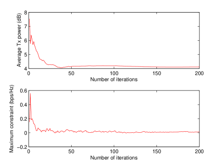
We use Example 3 to illustrate the fast convergence of SSCA-THP. Specifically, there are $K=8$ users and the target average rate for all users is set to be the same as $\gamma_{k}=2$ bps/Hz. Consider the DFT-based RF precoder. In Fig. 4, we plot the objective function (average transmit power) and the maximum constraint function (target average rate minus the minimum achieved average rate of users) versus the iteration number, respectively. It can be seen that SSCA-THP quickly converges to a point with all target average rates satisfied with high accuracy.

V-B Sum Throughput Maximization

Figure 5: Sum throughput (bps/Hz) versus the number of users $K$

Figure 6: Sum throughput versus the number of channel paths $N_{p}$

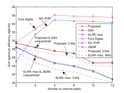
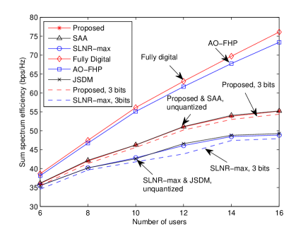
In Figs. 5 and 6, we plot the sum throughput versus the number of users $K$ and the number of channel paths $N_{p}$, respectively. The transmit power is set to be $P=10$ dB. For comparison, we also plot the sum throughput of the fully digital RZF beamforming [12] and the FHP algorithm based on alternating optimization (AO-FHP) in [16]. The proposed SSCA-THP achieves better performance than the existing THP algorithms (SLNR-max and JSDM). Moreover, as the number of users increases, the performance gap between SSCA-THP and SLNR-max/JSDM increases. Although SAA achieves similar performance to SSCA-THP after the channel sample collection phase, it has poor performance during the channel sample collection phase. Moreover, the per iteration complexity of SAA is much higher than that of SSCA-THP (CPU time: 10.00 s versus 0.06 s). The performance gap between the THP with statistical RF precoder and the FHP with real-time RF precoder (or fully digital RZF) is smaller when the number of users/channel paths is smaller. This is consistent with the analysis in [4]. Finally, it can be seen that with only three-bit quantization, the performance is already very close to the case without quantization.

V-C Proportional Fairness

Figure 7: PFS utility versus the number of users $K$

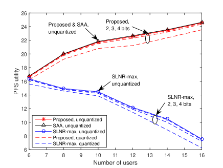
In Fig. 7, we plot the PFS utility versus the number of users $K$. The transmit power is set to be $P=10$ dB. Similar results to those in Fig. 5 can be observed. Moreover, when considering the PFS utility, the performance gap between SSCA-THP and SLNR-max is much larger since the fairness issue is not considered in the SLNR-max algorithm. Note that the PFS utility of SLNR-max decreases with the number of users. This is because, without considering the fairness, the minimum throughput of the users becomes much smaller as the number of users increases.

V-D Power Minimization

Figure 8: Average transmit power versus the target average rate

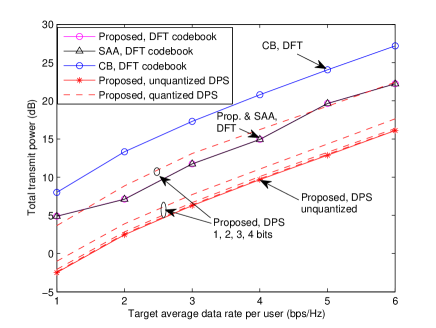
In Fig. 8, we plot the average transmit power versus the target average rate requirement $\gamma_{k}=\gamma,\forall k$ for a system with $K=8$ users. For any given target average rate $\gamma$, the proposed SSCA-THP with the DPS-based RF precoder achieves the lowest transmit power. The performance of the DPS-based RF precoder degrades as the number of quantization bits $B$ for each phase decreases. When $B=1$, the performance of the DPS-based RF precoder is similar to that of the DFT-based RF precoder optimized using the SSCA-THP or SAA algorithms, which is still much better than the DFT-based RF precoder optimized using the CB algorithm.

V-E Complexity Comparison

The complexity of SSCA-THP is dominated by the calculation of the Jacobian matrix $\mathbf{J}_{r}\left(\boldsymbol{x}^{l};\boldsymbol{H}^{l}\right)$, which has complexity order $O\left(MKS\right)$, and the quadratic optimization subproblems in (16) and (17), which has complexity order $O\left(Mm^{2}\right)$, as explained below. For given Lagrange multipliers, the complexity order of calculating the closed-form primal solution in (21) is $O\left(M\right)$. Using the ellipsoid method, the number of iterations required to achieve a given convergence accuracy $\epsilon$ for the dual problem (20) is $O\left(m^{2}\log\left(1/\epsilon\right)\right)$ [22]. Hence, the per-iteration complexity of SSCA-THP is $O\left(Mm^{2}\log\frac{1}{\epsilon}+MKS\right)$. In Table II, we compare the complexity order of SSCA-THP with SLNR-max in [5] and JSDM in [15] for the sum throughput maximization problem (i.e., $m=1$), where $L_{I}$ is the total number of iterations for SSCA-THP and Algorithm 1 in [5], respectively. The complexity order of both SLNR-max and JSDM increases with the number of BS antennas $M$ according to $M^{3}$ because they involve singular value decomposition (SVD) for the $M\times M$ channel covariance matrix. On the other hand, the complexity order of SSCA-THP only increases linearly with $M$, thanks to the closed-form solution in (21) for fixed Lagrange multipliers.

SSCA-THP	SLNR-max	JSDM
$O\left(L_{I}\left(M\log\frac{1}{\epsilon}+MKS\right)\right)$	$O\left(L_{I}M^{2}S+M^{3}\right)$	$O\left(M^{3}\right)$

Table II: Comparison of the complexity order for different algorithms.

VI Conclusion

In this paper, we first propose a general optimization formulation (7) for the design of THP in massive MIMO, which is applicable to different RF precoding structures/implementations and a wide range of application scenarios. Then we propose an online algorithmic framework called SSCA-THP to solve this general THP optimization problem. Specifically, at each iteration, quadratic surrogate functions are constructed for both objective and constraint functions based on a new channel sample. Then the next iterate is updated by solving the resulting quadratic optimization problem. We prove the convergence of SSCA-THP to stationary points. To the best of our knowledge, SSCA-THP is the first online and provably convergent algorithm to handle the general non-convex stochastic constraints considered in (7). Finally, we apply SSCA-THP to solve three important THP optimization problems and verify its advantages.

-A Jacobian Matrix of Instantaneous Rate

-A1 Jacobian Matrix for the Fully-connected DPS-based RF Precoder

In this case, we have $\boldsymbol{\phi}=\boldsymbol{\theta}=\mathbb{R}^{MS}$ and $\boldsymbol{x}=\left[\boldsymbol{\theta}^{T},\boldsymbol{p}^{T},\alpha,\boldsymbol{\beta}^{T}\right]^{T}$. We first define some useful notations:

$$\boldsymbol{A}_{k,i} =2\boldsymbol{H}_{F}^{H}\mathfrak{S}\left[\boldsymbol{H}\boldsymbol{F}\boldsymbol{F}^{H}\boldsymbol{h}_{k}\boldsymbol{h}_{k}^{H}\overline{\boldsymbol{G}}\boldsymbol{P}_{i}\boldsymbol{\Lambda}\right]\boldsymbol{H}_{F}\boldsymbol{F}$$

$$-2\mathfrak{S}\left[\boldsymbol{h}_{k}\boldsymbol{h}_{k}^{H}\overline{\boldsymbol{G}}\boldsymbol{P}_{i}\boldsymbol{\Lambda}\boldsymbol{H}_{F}\right]\boldsymbol{F},$$

$$\boldsymbol{E}_{i} =2\boldsymbol{H}_{F}^{H}\mathfrak{S}\left[\boldsymbol{H}\boldsymbol{F}\boldsymbol{F}^{H}\overline{\boldsymbol{G}}\boldsymbol{I}_{i}\right]\boldsymbol{H}_{F}\boldsymbol{F}-2\mathfrak{S}\left[\overline{\boldsymbol{G}}\boldsymbol{I}_{i}\boldsymbol{H}_{F}\right]\boldsymbol{F},$$

$$e_{k,i} =\left[\boldsymbol{H}_{F}\boldsymbol{F}\boldsymbol{F}^{H}\boldsymbol{h}_{k}\boldsymbol{h}_{k}^{H}\boldsymbol{F}\boldsymbol{F}^{H}\boldsymbol{H}_{F}^{H}\boldsymbol{P}_{i}\boldsymbol{\Lambda}^{2}\right]_{i,i},$$

where $\boldsymbol{H}_{F}=\boldsymbol{B}\boldsymbol{H}$ with $\boldsymbol{B}=\left(\boldsymbol{H}\boldsymbol{F}\boldsymbol{F}^{H}\boldsymbol{H}^{H}+\alpha\boldsymbol{I}\right)^{-1}$, and $\boldsymbol{P}_{i}$ ($\boldsymbol{I}_{i}$) denotes a $K\times K$ matrix with $\left[\boldsymbol{P}_{i}\right]_{i,i}=p_{i}$ ($\left[\boldsymbol{I}_{i}\right]_{i,i}=1$) and all other elements being zero. Then using the matrix calculus, it can be shown that the gradients of $r_{k}\left(\boldsymbol{\theta},\boldsymbol{p},\alpha;\boldsymbol{H}\right)$ w.r.t. $\boldsymbol{\theta}$, $\boldsymbol{p}$ and $\alpha$ are respectively given by

$$\nabla_{\boldsymbol{\theta}}r_{k}\left(\boldsymbol{\theta},\boldsymbol{p},\alpha;\boldsymbol{H}\right) =\frac{\sum_{i}\boldsymbol{a}_{k,i}^{\theta}}{\varGamma_{k}}-\frac{\sum_{i\neq k}\boldsymbol{a}_{k,i}^{\theta}}{\varGamma_{-k}}$$ (24)

$$\nabla_{\boldsymbol{p}}r_{k}\left(\boldsymbol{\theta},\boldsymbol{p},\alpha;\boldsymbol{H}\right) =\frac{\sum_{i}\boldsymbol{a}_{k,i}^{p}}{\varGamma_{k}}-\frac{\sum_{i\neq k}\boldsymbol{a}_{k,i}^{p}}{\varGamma_{-k}},$$ (25)

$$\nabla_{\alpha}r_{k}\left(\boldsymbol{\theta},\boldsymbol{p},\alpha;\boldsymbol{H}\right) =\frac{\sum_{i}a_{k,i}^{\alpha}}{\varGamma_{k}}-\frac{\sum_{i\neq k}a_{k,i}^{\alpha}}{\varGamma_{-k}},$$ (26)

where $\varGamma_{k}=\sum_{i}p_{i}\left|\boldsymbol{h}_{k}^{H}\boldsymbol{F}\boldsymbol{g}_{i}\right|^{2}+1$, $\varGamma_{-k}=\sum_{i\neq k}p_{i}\left|\boldsymbol{h}_{k}^{H}\boldsymbol{F}\boldsymbol{g}_{i}\right|^{2}+1$,

$$\boldsymbol{a}_{k,i}^{\theta} =\textrm{Vec}\left(\mathfrak{R}\left[\sqrt{-1}\boldsymbol{F}^{*}\circ\boldsymbol{A}_{k,i}\right]\right)-e_{k,i}\textrm{Vec}\left(\mathfrak{R}\left[\sqrt{-1}\boldsymbol{F}^{*}\circ\boldsymbol{E}_{i}\right]\right),$$

$$\boldsymbol{a}_{k,i}^{p} =\textrm{Diag}\left(\overline{\boldsymbol{G}}^{H}\boldsymbol{h}_{k}\boldsymbol{h}_{k}^{H}\overline{\boldsymbol{G}}\boldsymbol{\Lambda}_{i}\right),$$

$$a_{k,i}^{\alpha} =e_{k,i}2\mathfrak{R}\left[Tr\left(\overline{\boldsymbol{G}}\boldsymbol{I}_{i}\boldsymbol{B}\overline{\boldsymbol{G}}^{H}\right)\right]-2\mathfrak{R}\left[\boldsymbol{h}_{k}^{H}\overline{\boldsymbol{G}}\boldsymbol{P}_{i}\boldsymbol{\Lambda}_{i}\boldsymbol{B}\overline{\boldsymbol{G}}^{H}\boldsymbol{h}_{k}\right].$$

Therefore, for given channel state $\boldsymbol{H}$, the Jacobian matrix of the instantaneous rate vector $\boldsymbol{r}\left(\boldsymbol{\theta},\boldsymbol{p},\alpha;\boldsymbol{H}\right)$ w.r.t. $\boldsymbol{x}$ is

$$\mathbf{J}_{r}\left(\boldsymbol{x};\boldsymbol{H}\right)=\left[\begin{array}[]{cccc}\nabla_{\boldsymbol{\theta}}r_{1}&\nabla_{\boldsymbol{\theta}}r_{2}&\cdots&\nabla_{\boldsymbol{\theta}}r_{K}\\ \nabla_{\boldsymbol{p}}r_{1}&\nabla_{\boldsymbol{p}}r_{2}&\cdots&\nabla_{\boldsymbol{p}}r_{K}\\ \nabla_{\alpha}r_{1}&\nabla_{\alpha}r_{2}&\cdots&\nabla_{\alpha}r_{K}\\ \boldsymbol{0}&\boldsymbol{0}&\boldsymbol{0}&\boldsymbol{0}\end{array}\right],$$ (27)

where the bottom submatrix is zero because $\nabla_{\boldsymbol{\beta}}r_{k}=\boldsymbol{0},\forall k$. Note that we have omitted $\left(\boldsymbol{\theta},\boldsymbol{p},\alpha;\boldsymbol{H}\right)$ in the gradient expressions for simplicity of notation.

-A2 Jacobian Matrix for the Fully-connected Codebook-based RF Precoder

In this case, we have $\boldsymbol{\phi}=\boldsymbol{d}=\left[0,1\right]^{N}$ and $\boldsymbol{x}=\left[\boldsymbol{d}^{T},\boldsymbol{p}^{T},\alpha,\boldsymbol{\beta}^{T}\right]^{T}$. Using the matrix calculus, it can be shown that the gradients of $r_{k}\left(\boldsymbol{d},\boldsymbol{p},\alpha;\boldsymbol{H}\right)$ w.r.t. $\boldsymbol{p}$ and $\alpha$ are given by (25) and (26), respectively; and the gradient of $r_{k}\left(\boldsymbol{d},\boldsymbol{p},\alpha;\boldsymbol{H}\right)$ w.r.t. $\boldsymbol{d}$ is

$$\nabla_{\boldsymbol{d}}r_{k}\left(\boldsymbol{\theta},\boldsymbol{p},\alpha;\boldsymbol{H}\right)=\frac{\sum_{i}\boldsymbol{a}_{k,i}^{d}}{\varGamma}-\frac{\sum_{i\neq k}\boldsymbol{a}_{k,i}^{d}}{\varGamma_{k}},$$

where $\boldsymbol{a}_{k,i}^{d}=-\frac{1}{2}\textrm{Diag}\left(\boldsymbol{C}^{H}\boldsymbol{A}_{k,i}\boldsymbol{C}\right)+\frac{e_{k,i}}{2}\textrm{Diag}\left(\boldsymbol{C}^{H}\boldsymbol{E}_{i}\boldsymbol{C}\right)$. Finally, for given channel state $\boldsymbol{H}$, the Jacobian matrix of the instantaneous rate vector $\boldsymbol{r}\left(\boldsymbol{d},\boldsymbol{p},\alpha;\boldsymbol{H}\right)$ w.r.t. $\boldsymbol{x}$ is given by (27) with $\nabla_{\boldsymbol{\theta}}r_{k},\forall k$ replaced by $\nabla_{\boldsymbol{d}}r_{k},\forall k$.

The Jacobian matrix of the instantaneous rate vector for the partially-connected structure can be obtained similarly. The details are omitted for conciseness.

-B Proof of Lemma 1

The proof relies on the following lemma.

Lemma 3.

Under Assumption 2, we have

$$\lim_{l\rightarrow\infty}\left|\bar{f}_{i}^{l}\left(\boldsymbol{x}^{l}\right)-f_{i}\left(\boldsymbol{x}^{l}\right)\right| =0,$$ (28)

$$\lim_{l\rightarrow\infty}\left\|\nabla\bar{f}_{i}^{l}\left(\boldsymbol{x}^{l}\right)-\nabla f_{i}\left(\boldsymbol{x}^{l}\right)\right\| =0,$$ (29)

$$\lim_{l_{1},l_{2}\rightarrow\infty}\bar{f}_{i}^{l_{1}}\left(\boldsymbol{x}^{l_{1}}\right)-\bar{f}_{i}^{l_{2}}\left(\boldsymbol{x}^{l_{2}}\right) \leq C\left\|\boldsymbol{x}^{l_{1}}-\boldsymbol{x}^{l_{2}}\right\|.$$ (30)

for $i=0,...,m$ w.p.1., where $C>0$ is some constant.

Proof:

It follows from the law of large numbers and the central limit theorem that

$$\hat{\boldsymbol{r}}^{l}\overset{a.s.}{\rightarrow}\overline{\boldsymbol{r}}^{l},\> \mathbb{E}\left\|\hat{\boldsymbol{r}}^{l}-\overline{\boldsymbol{r}}^{l}\right\|=O\left(\frac{1}{\sqrt{l}}\right),$$ (31)

where $\overline{\boldsymbol{r}}^{l}=\overline{\boldsymbol{r}}\left(\boldsymbol{\phi}^{l},\boldsymbol{p}^{l},\alpha^{l}\right)$. Then (28) follows from (31).

On the other hand, (29) is a consequence of [24], Lemma 1. It is easy to verify that the technical conditions (a), (b), (d) and (e) therein are satisfied. In the following, we prove that condition (c) in [24], Lemma 1 is also satisfied. Let $\overline{\nabla}_{\xi}^{l}h_{i}=\nabla_{\xi}h_{i}\left(\overline{\boldsymbol{r}}^{l},\boldsymbol{x}^{l}\right)$ and $\hat{\nabla}_{\xi}^{l}h_{i}=\nabla_{\xi}h_{i}\left(\hat{\boldsymbol{r}}^{l},\boldsymbol{x}^{l}\right)$ for $\xi\in\left\{\overline{\boldsymbol{r}},\boldsymbol{x}\right\}$. Let $\mathbf{J}_{\overline{r}}\left(\boldsymbol{x}^{l}\right)=\mathbb{E}\left[\mathbf{J}_{r}\left(\boldsymbol{x}^{l},\boldsymbol{H}^{l}\right)\right]$ denote the Jacobian matrix of the average rate vector $\overline{\boldsymbol{r}}\left(\boldsymbol{\phi}^{l},\boldsymbol{p}^{l},\alpha^{l}\right)$ at point $\boldsymbol{x}^{l}$. Then we have

$$\nabla f_{i}\left(\boldsymbol{x}^{l}\right)=\mathbf{J}_{\overline{r}}\left(\boldsymbol{x}^{l}\right)\overline{\nabla}_{\overline{\boldsymbol{r}}}^{l}h_{i}+\overline{\nabla}_{\boldsymbol{x}}^{l}h_{i}.$$ (32)

It follows from (32) and (31) that

$$\left\|\mathbb{E}\left[\hat{\mathbf{u}}_{i}^{l}\right]-\nabla f_{i}\left(\boldsymbol{x}^{l}\right)\right\| \leq\mathbb{E}\left\|\mathbf{J}_{r}\left(\boldsymbol{x}^{l},\boldsymbol{H}^{l}\right)\left(\hat{\nabla}_{\overline{\boldsymbol{r}}}^{l}h_{i}-\overline{\nabla}_{\overline{\boldsymbol{r}}}^{l}h_{i}\right)\right\|$$

$$+ \mathbb{E}\left\|\hat{\nabla}_{\boldsymbol{x}}^{l}h_{i}-\overline{\nabla}_{\boldsymbol{x}}^{l}h_{i}\right\|$$

$$\overset{\textrm{a}}{=} O\left(\left\|\hat{\boldsymbol{r}}^{l}-\overline{\boldsymbol{r}}^{l}\right\|\right)=O\left(\frac{1}{\sqrt{l}}\right),$$ (33)

where (33-a) holds because $\nabla h_{i}$ are Lipschitz continuous and $\mathbf{J}_{r}\left(\boldsymbol{x}^{l},\boldsymbol{H}^{l}\right)$ are bounded w.p.1. From (33) and $\sum_{l=1}^{\infty}\rho^{l}l^{-0.5}<\infty$, we have $\sum_{l=1}^{\infty}\rho^{l}\left\|\mathbb{E}\left[\hat{\mathbf{u}}_{i}^{l}\right]-\nabla f_{i}\left(\boldsymbol{x}^{l}\right)\right\|<\infty$, which implies that the technical condition (c) in [24], Lemma 1 is satisfied.

Finally, (30) follows from the Lipschitz continuity of $h_{i}$. This completes the proof. ∎

From Lemma 3 and (31), the families of functions $\left\{\bar{f}_{i}^{l_{j}}\left(\boldsymbol{x}\right)\right\}$ converge to $\left\{\hat{f}_{i}\left(\boldsymbol{x}\right)\right\}$ almost surely.

-C Proof of Lemma 2

1. We first prove $\limsup_{l\rightarrow\infty}f\left(\boldsymbol{x}^{l}\right)\leq 0$ w.p.1., where $f\left(\boldsymbol{x}\right)=\max_{i\in\left\{1,...,m\right\}}f_{i}\left(\boldsymbol{x}\right)$.

Let $\mathcal{T}_{\epsilon}=\left\{l:\>f\left(\boldsymbol{x}^{l}\right)\geq\epsilon\right\}$ for any $\epsilon>0$. We show that $\mathcal{T}_{\epsilon}$ is a finite set by contradiction.

Suppose $\mathcal{T}_{\epsilon}$ is infinite. We first show that $\liminf_{l\in\mathcal{T}_{\epsilon},l\rightarrow\infty}\left\|\bar{\boldsymbol{x}}^{l}-\boldsymbol{x}^{l}\right\|>0$ by contradiction. Suppose $\liminf_{l\in\mathcal{T}_{\epsilon},l\rightarrow\infty}\left\|\bar{\boldsymbol{x}}^{l}-\boldsymbol{x}^{l}\right\|=0$. Then there exists a subsequence $l^{j}\in\mathcal{T}_{\epsilon}$ such that $\lim_{j\rightarrow\infty}\left\|\bar{\boldsymbol{x}}^{l_{j}}-\boldsymbol{x}^{l_{j}}\right\|=0$. Let $\boldsymbol{x}^{\circ}$ denote a limiting point of the subsequence $\left\{\boldsymbol{x}^{l_{j}}\right\}$, and let $\hat{f}_{i}\left(\boldsymbol{x}\right),\forall i$ be the converged surrogate functions as defined in Lemma 1. According to the update rule of Algorithm 1, there are two cases.

Case 1: $\boldsymbol{x}^{\circ}$ is the optimal solution of the following convex optimization problem:

$$\underset{\boldsymbol{x}}{\text{min}}\> \hat{f}_{0}\left(\boldsymbol{x}\right)$$ (34)

$$s.t.\> \hat{f}_{i}\left(\boldsymbol{x}\right)\leq 0,i=1,....,m.$$

In this case, we have $f\left(\boldsymbol{x}^{\circ}\right)=\max_{i\in\left\{1,...,m\right\}}\hat{f}_{i}\left(\boldsymbol{x}^{\circ}\right)\leq 0$, which contradicts the definition of $\mathcal{T}_{\epsilon}$.

Case 2: $\boldsymbol{x}^{\circ}$ is the optimal solution of the following convex optimization problem:

$$\underset{\boldsymbol{x},\nu}{\text{min}}\> \nu$$ (35)

$$s.t.\> \hat{f}_{i}\left(\boldsymbol{x}\right)\leq\nu,i=1,....,m.$$

Since the Slater condition is satisfied (by choosing a sufficiently large $\nu$, we can always find a point $\boldsymbol{x}\in\mathcal{X}$ such that $\hat{f}_{i}\left(\boldsymbol{x}\right)<\nu,i=1,....,m$), the KKT condition of the problem (35) implies that there exist $\lambda_{1},...,\lambda_{m}$ such that

$$\sum_{i}\lambda_{i}\nabla\hat{f}_{i}\left(\boldsymbol{x}^{\circ}\right) =\boldsymbol{0},$$

$$1-\sum_{i}\lambda_{i} =0,$$

$$\hat{f}_{i}\left(\boldsymbol{x}^{\circ}\right) \leq\nu,\>\forall i=1,...,m,$$

$$\lambda_{i}\left(\hat{f}_{i}\left(\boldsymbol{x}^{\circ}\right)-\nu\right) =0,\>\forall i=1,...,m.$$ (36)

It follows from Lemma 1 and (36) that $\boldsymbol{x}^{\circ}$ also satisfies the KKT condition of Problem (22). By Assumption 1, we have $f_{i}\left(\boldsymbol{x}^{\circ}\right)\leq 0,i=1,...,m$, which again contradicts the definition of $\mathcal{T}_{\epsilon}$.

Therefore, $\liminf_{l\in\mathcal{T}_{\epsilon},l\rightarrow\infty}\left\|\bar{\boldsymbol{x}}^{l}-\boldsymbol{x}^{l}\right\|>0$; i.e., there exists a sufficiently large $l_{\epsilon}$ such that

$$\left\|\bar{\boldsymbol{x}}^{l}-\boldsymbol{x}^{l}\right\|\geq\epsilon^{{}^{\prime}},\forall l\in\mathcal{T}_{\epsilon}^{{}^{\prime}},$$ (37)

where $\epsilon^{{}^{\prime}}>0$ is some constant and $\mathcal{T}_{\epsilon}^{{}^{\prime}}=\mathcal{T}_{\epsilon}\cap\left\{l\geq l_{\epsilon}\right\}$.

Define function $\bar{f}^{l}\left(\boldsymbol{x}\right)=\max_{i\in\left\{1,...,m\right\}}\bar{f}_{i}^{l}\left(\boldsymbol{x}\right)$. From the definition of $\bar{f}_{i}^{l}\left(\boldsymbol{x}\right)$ in (14), $\bar{f}_{i}^{l}\left(\boldsymbol{x}\right)$ is strongly convex, and thus

$$\nabla^{T}\bar{f}_{i}^{l}\left(\boldsymbol{x}^{l}\right)\boldsymbol{d}^{l}\leq-\eta\left\|\boldsymbol{d}^{l}\right\|^{2}+\bar{f}_{i}^{l}\left(\bar{\boldsymbol{x}}^{l}\right)-\bar{f}_{i}^{l}\left(\boldsymbol{x}^{l}\right),$$ (38)

where $\boldsymbol{d}^{l}=\bar{\boldsymbol{x}}^{l}-\boldsymbol{x}^{l}$, and $\eta>0$ is some constant. From Assumption 1, the gradient of $f_{i}\left(\boldsymbol{x}\right)$ is Lipschitz continuous, and thus there exists $L_{f}>0$ such that

$$f_{i}\left(\boldsymbol{x}^{l+1}\right) \leq f_{i}\left(\boldsymbol{x}^{l}\right)+\gamma^{l}\nabla^{T}f_{i}\left(\boldsymbol{x}^{l}\right)\boldsymbol{d}^{l}+L_{f}\left(\gamma^{l}\right)^{2}\left\|\boldsymbol{d}^{l}\right\|^{2}$$

$$=f\left(\boldsymbol{x}^{l}\right)+L_{f}\left(\gamma^{l}\right)^{2}\left\|\boldsymbol{d}^{l}\right\|^{2}+f_{i}\left(\boldsymbol{x}^{l}\right)-f\left(\boldsymbol{x}^{l}\right)$$

$$+\gamma^{l}\left(\nabla^{T}\bar{f}_{i}^{l}\left(\boldsymbol{x}^{l}\right)+\nabla^{T}f_{i}\left(\boldsymbol{x}^{l}\right)-\nabla^{T}\bar{f}_{i}^{l}\left(\boldsymbol{x}^{l}\right)\right)\boldsymbol{d}^{l}$$

$$\overset{\textrm{a}}{\leq}f\left(\boldsymbol{x}^{l}\right)+f_{i}\left(\boldsymbol{x}^{l}\right)-f\left(\boldsymbol{x}^{l}\right)-\eta\gamma^{l}\left\|\boldsymbol{d}^{l}\right\|^{2}$$

$$+\gamma^{l}\left(\bar{f}_{i}^{l}\left(\bar{\boldsymbol{x}}^{l}\right)-\bar{f}_{i}^{l}\left(\boldsymbol{x}^{l}\right)\right)+o\left(\gamma^{l}\right)$$

$$\leq f\left(\boldsymbol{x}^{l}\right)-\eta\gamma^{l}\left\|\boldsymbol{d}^{l}\right\|^{2}+o\left(\gamma^{l}\right),\forall i=1,...,m,$$ (39)

where $o\left(\gamma^{l}\right)$ means that $\lim_{l\rightarrow\infty}o\left(\gamma^{l}\right)/\gamma^{l}=0$. In (39-a), we used (38) and $\lim_{l\rightarrow\infty}\left\|\nabla^{T}f_{i}\left(\boldsymbol{x}^{l}\right)-\nabla^{T}\bar{f}_{i}^{l}\left(\boldsymbol{x}^{l}\right)\right\|=0$, and the last inequality follows from $f_{i}\left(\boldsymbol{x}^{l}\right)\leq f\left(\boldsymbol{x}^{l}\right)$, $\liminf_{l\rightarrow\infty}f\left(\boldsymbol{x}^{l}\right)-\bar{f}_{i}^{l}\left(\bar{\boldsymbol{x}}^{l}\right)\geq 0$, and $\lim_{l\rightarrow\infty}\left\|f_{i}\left(\boldsymbol{x}^{l}\right)-\bar{f}_{i}^{l}\left(\boldsymbol{x}^{l}\right)\right\|=0$. Since (39) holds for all $i=1,...,m$, by choosing a sufficiently large $l_{\epsilon}$, we have

$$f\left(\boldsymbol{x}^{l+1}\right)-f\left(\boldsymbol{x}^{l}\right) \leq-\gamma^{l}\overline{\eta}\left\|\boldsymbol{d}^{l}\right\|^{2}$$

$$\leq-\gamma^{l}\overline{\eta}\epsilon^{{}^{\prime}},\forall l\in\mathcal{T}_{\epsilon}^{{}^{\prime}},$$ (40)

for some $\overline{\eta}>0$. Moreover, from Assumption 1, the directional derivative of $f\left(\boldsymbol{x}\right)$ is uniformly bounded, and thus there exists a constant $C$ such that

$$\left|f\left(\boldsymbol{x}^{l+1}\right)-f\left(\boldsymbol{x}^{l}\right)\right|\leq C\left\|\boldsymbol{x}^{l+1}-\boldsymbol{x}^{l}\right\|\leq C^{{}^{\prime}}\gamma^{l},$$ (41)

for some $C^{{}^{\prime}}>0$. Finally, it follows from (40) and (41) that

$$f\left(\boldsymbol{x}^{l}\right)\leq 2\epsilon,\forall l\geq l_{\epsilon}.$$ (42)

Since (42) is true for any $\epsilon>0$, it follows that $\limsup_{l\rightarrow\infty}f\left(\boldsymbol{x}^{l}\right)\leq 0$.

2. Then we prove that $\lim_{l\rightarrow\infty}\left\|\bar{\boldsymbol{x}}^{l}-\boldsymbol{x}^{l}\right\|=0,$ w.p.1.

2.1: We first prove that $\liminf_{l\rightarrow\infty}\left\|\bar{\boldsymbol{x}}^{l}-\boldsymbol{x}^{l}\right\|=0$ w.p.1.

Note that the feasible problem in (17) is strictly convex, and thus the solution is uniquely given by $\bar{\boldsymbol{x}}^{l}$. Therefore, when a feasible update is performed at iteration $l$, we have $\bar{f}^{l}\left(\bar{\boldsymbol{x}}^{l}\right)\geq 0$ and

$$\bar{\boldsymbol{x}}^{l}=\underset{\boldsymbol{x}}{\text{argmin}\>} \bar{f}_{0}^{l}\left(\boldsymbol{x}\right)$$

$$s.t.\> \bar{f}_{i}^{l}\left(\boldsymbol{x}\right)\leq\bar{f}^{l}\left(\bar{\boldsymbol{x}}^{l}\right),i=1,....,m.$$

As a result, $\bar{\boldsymbol{x}}^{l}$ can be expressed in a unified way as

$$\bar{\boldsymbol{x}}^{l}=\underset{\boldsymbol{x}}{\text{argmin}}\> \bar{f}_{0}^{l}\left(\boldsymbol{x}\right)$$ (43)

$$s.t.\> \bar{f}_{i}^{l}\left(\boldsymbol{x}\right)\leq\nu^{l},i=1,....,m,$$

where $\nu^{l}=0$ when an objective update is performed and $\nu^{l}=\bar{f}^{l}\left(\bar{\boldsymbol{x}}^{l}\right)$ when a feasible update is performed. Since $\lim_{l\rightarrow\infty}\left|\bar{f}^{l}\left(\boldsymbol{x}^{l}\right)-f\left(\boldsymbol{x}^{l}\right)\right|=0$, $\bar{f}^{l}\left(\bar{\boldsymbol{x}}^{l}\right)\leq\bar{f}^{l}\left(\boldsymbol{x}^{l}\right)$, and we have proved that $\limsup_{l\rightarrow\infty}f\left(\boldsymbol{x}^{l}\right)\leq 0$, it follows that $\lim_{l\rightarrow\infty}\nu^{l}=0$. Let $\hat{\boldsymbol{x}}^{l}$ denote the projection of $\boldsymbol{x}^{l}$ on to the feasible set of Problem (43). Then it follows from $\lim_{l\rightarrow\infty}\nu^{l}=0$, $\limsup_{l\rightarrow\infty}\bar{f}^{l}\left(\boldsymbol{x}^{l}\right)=\limsup_{t\rightarrow\infty}f\left(\boldsymbol{x}^{l}\right)\leq 0$, and the strong convexity of $\bar{f}^{l}\left(\boldsymbol{x}^{l}\right)$ that

$$\lim_{l\rightarrow\infty}\left\|\boldsymbol{x}^{l}-\hat{\boldsymbol{x}}^{l}\right\|=0.$$ (44)

From the definition of $\bar{f}_{0}^{l}\left(\boldsymbol{x}\right)$ in (14), $\bar{f}_{0}^{l}\left(\boldsymbol{x}\right)$ is uniformly strongly convex, and thus

$$\nabla^{T}\bar{f}_{0}^{l}\left(\boldsymbol{x}^{l}\right)\boldsymbol{d}^{l} \leq-\eta\left\|\boldsymbol{d}^{l}\right\|^{2}+\bar{f}_{0}^{l}\left(\bar{\boldsymbol{x}}^{l}\right)-\bar{f}_{0}^{l}\left(\boldsymbol{x}^{l}\right)$$

$$=-\eta\left\|\boldsymbol{d}^{l}\right\|^{2}+\bar{f}_{0}^{l}\left(\bar{\boldsymbol{x}}^{l}\right)-\bar{f_{0}}^{l}\left(\hat{\boldsymbol{x}}^{l}\right)$$

$$+\bar{f_{0}}^{l}\left(\hat{\boldsymbol{x}}^{l}\right)-\bar{f}_{0}^{l}\left(\boldsymbol{x}^{l}\right)$$

$$\leq-\eta\left\|\boldsymbol{d}^{l}\right\|^{2}+e\left(l\right),$$ (45)

for some $\eta>0$, where $\boldsymbol{d}^{l}=\bar{\boldsymbol{x}}^{l}-\boldsymbol{x}^{l}$, $\lim_{l\rightarrow\infty}e\left(l\right)=0$, and the last equality follows from (44). From Assumption 1, the gradient of $f_{0}\left(\boldsymbol{x}\right)$ is Lipschitz continuous, and thus there exists $L_{0}>0$ such that

$$f_{0}\left(\boldsymbol{x}^{l+1}\right) \leq f_{0}\left(\boldsymbol{x}^{l}\right)+\gamma^{l}\nabla^{T}f_{0}\left(\boldsymbol{x}^{l}\right)\boldsymbol{d}^{l}+L_{0}\left(\gamma^{l}\right)^{2}\left\|\boldsymbol{d}^{l}\right\|^{2}$$

$$=f_{0}\left(\boldsymbol{x}^{l}\right)+L_{0}\left(\gamma^{l}\right)^{2}\left\|\boldsymbol{d}^{l}\right\|^{2}$$

$$+\gamma^{l}\left(\nabla^{T}f_{0}\left(\boldsymbol{x}^{l}\right)-\nabla^{T}\bar{f_{0}}^{l}\left(\boldsymbol{x}^{l}\right)+\nabla^{T}\bar{f_{0}}^{l}\left(\boldsymbol{x}^{l}\right)\right)\boldsymbol{d}^{l}$$

$$\leq f_{0}\left(\boldsymbol{x}^{l}\right)-\gamma^{t}\eta\left\|\boldsymbol{d}^{l}\right\|^{2}+o\left(\gamma^{l}\right),$$

where in the last inequality, we used (45) and $\lim_{l\rightarrow\infty}\left\|\nabla^{T}f_{0}\left(\boldsymbol{x}^{l}\right)-\nabla^{T}\bar{f}_{0}^{l}\left(\boldsymbol{x}^{l}\right)\right\|=0$. Let us show by contradiction that w.p.1. $\liminf_{l\rightarrow\infty}\left\|\bar{\boldsymbol{x}}^{l}-\boldsymbol{x}^{l}\right\|=0$. Suppose $\liminf_{l\rightarrow\infty}\left\|\bar{\boldsymbol{x}}^{l}-\boldsymbol{x}^{l}\right\|\geq\chi>0$ with a positive probability. Then we can find a realization such that $\left\|\boldsymbol{d}^{l}\right\|\geq\chi$ at the same time for all $l$. We focus next on such a realization. By choosing a sufficiently large $l_{0}$, there exists $\overline{\eta}>0$ such that

$$f_{0}\left(\boldsymbol{x}^{l+1}\right)-f_{0}\left(\boldsymbol{x}^{l}\right) \leq-\gamma^{l}\overline{\eta}\left\|\boldsymbol{d}^{l}\right\|^{2},\forall l\geq l_{0}.$$ (46)

It follows from (46) that

$$f_{0}\left(\boldsymbol{x}^{l}\right)-f_{0}\left(\boldsymbol{x}^{l_{0}}\right)\leq-\overline{\eta}\chi^{2}\sum_{j=l_{0}}^{l}\left(\gamma^{j}\right)^{2},$$

which, in view of $\sum_{j=l_{0}}^{\infty}\left(\gamma^{j}\right)^{2}=\infty$, contradicts the boundedness of $\left\{f_{0}\left(\boldsymbol{x}^{l}\right)\right\}$. Therefore it must be $\liminf_{l\rightarrow\infty}\left\|\bar{\boldsymbol{x}}^{l}-\boldsymbol{x}^{l}\right\|=0$ w.p.1.

2.2: Then we prove that $\limsup_{l\rightarrow\infty}\left\|\bar{\boldsymbol{x}}^{l}-\boldsymbol{x}^{l}\right\|=0$ w.p.1.

We first prove a useful lemma.

Lemma 4.

There exists a constant $\hat{L}>0$ such that

$$\left\|\bar{\boldsymbol{x}}^{l_{1}}-\bar{\boldsymbol{x}}^{l_{2}}\right\|\leq\hat{L}\left\|\boldsymbol{x}^{l_{1}}-\boldsymbol{x}^{l_{2}}\right\|+e\left(l_{1},l_{2}\right),$$

where $\lim_{l_{1},l_{2}\rightarrow\infty}e\left(l_{1},l_{2}\right)=0$.

Proof:

From Lemma 3, we have

$$\left|\bar{f}_{i}^{l_{1}}\left(\boldsymbol{x}\right)-\bar{f}_{i}^{l_{2}}\left(\boldsymbol{x}\right)\right|\leq C\left\|\boldsymbol{x}^{l_{1}}-\boldsymbol{x}^{l_{2}}\right\|+e^{{}^{\prime}}\left(l_{1},l_{2}\right),$$ (47)

for all $\boldsymbol{x}\in\mathcal{X}$ and $i=0,1,...,m$, where $\lim_{l_{1},l_{2}\rightarrow\infty}e^{{}^{\prime}}\left(l_{1},l_{2}\right)=0$. Then it follows from (47) and (43), and the Lipschitz continuity and strong convexity of $\bar{f}_{i}^{l}\left(\boldsymbol{x}\right),\forall i$ that

$$\left\|\bar{\boldsymbol{x}}^{l_{1}}-\bar{\boldsymbol{x}}^{l_{2}}\right\|\leq C_{1}C\left\|\boldsymbol{x}^{l_{1}}-\boldsymbol{x}^{l_{2}}\right\|+C_{1}e^{{}^{\prime}}\left(l_{1},l_{2}\right)+C_{2}\nu^{l}$$ (48)

for some constant $C_{1},C_{2}>0$. Finally, Lemma 4 follows from (48) immediately. ∎

Using Lemma 4 and following the same analysis as that in [10], Proof of Theorem 1, it can be shown that $\limsup_{l\rightarrow\infty}\left\|\bar{\boldsymbol{x}}^{l}-\boldsymbol{x}^{l}\right\|=0$ w.p.1. This completes the proof.

-D Proof of Theorem 1

According to Lemma 1, Lemma 2, and (43), $\boldsymbol{x}^{*}$ must be the optimal solution of the following convex optimization problem almost surely:

$$\underset{\boldsymbol{x}}{\text{min}}\> \hat{f}_{0}\left(\boldsymbol{x}\right)$$ (49)

$$s.t.\> \hat{f}_{i}\left(\boldsymbol{x}\right)\leq 0,i=1,....,m.$$

Since the Slater condition is satisfied, the KKT condition of Problem (49) implies that there exist $\lambda_{1},...,\lambda_{m}$ such that

$$\nabla\hat{f}_{0}\left(\boldsymbol{x}\right)+\sum_{i}\lambda_{i}\nabla\hat{f}_{i}\left(\boldsymbol{x}^{*}\right) =\boldsymbol{0},$$

$$\hat{f}_{i}\left(\boldsymbol{x}^{*}\right) \leq 0,\>\forall i=1,...,m,$$

$$\lambda_{i}\hat{f}_{i}\left(\boldsymbol{x}^{*}\right) =0,\>\forall i=1,...,m.$$ (50)

It follows from Lemma 1 and (50) that $\boldsymbol{x}^{*}$ also satisfies the KKT condition of Problem (7). This completes the proof.

References

• [1] O. E. Ayach, S. Rajagopal, S. Abu-Surra, Z. Pi, and R. W. Heath, “Spatially sparse precoding in millimeter wave MIMO systems,” IEEE Trans. Wireless Commun., vol. 13, no. 3, pp. 1499–1513, Mar. 2014.
• [2] L. Liang, W. Xu, and X. Dong, “Low-complexity hybrid precoding in massive multiuser MIMO systems,” IEEE Wireless Commun. Lett., vol. 3, no. 6, pp. 653–656, Dec. 2014.
• [3] A. Alkhateeb, G. Leus, and R. Heath, “Limited feedback hybrid precoding for multi-user millimeter wave systems,” IEEE Trans. Wireless Commun., vol. 14, no. 11, pp. 6481–6494, Nov. 2015.
• [4] A. Liu and V. K. N. Lau, “Impact of CSI knowledge on the codebook-based hybrid beamforming in massive MIMO,” IEEE Transactions on Signal Processing, vol. 64, no. 24, pp. 6545–6556, Dec 2016.
• [5] S. Park, J. Park, A. Yazdan, and R. W. Heath, “Exploiting spatial channel covariance for hybrid precoding in massive MIMO systems,” IEEE Trans. Signal Processing, vol. 65, no. 14, pp. 3818–3832, July 2017.
• [6] A. Liu and V. K. N. Lau, “Phase only RF precoding for massive MIMO systems with limited RF chains,” IEEE Trans. Signal Processing, vol. 62, no. 17, pp. 4505–4515, Sept. 2014.
• [7] ——, “Two-stage constant-envelope precoding for low-cost massive MIMO systems,” IEEE Trans. Signal Processing, vol. 64, no. 2, pp. 485–494, Jan. 2016.
• [8] A. K. Sadek, W. Su, and K. J. R. Liu, “Transmit beamforming for space-frequency coded MIMO-OFDM systems with spatial correlation feedback,” IEEE Trans. Commun., vol. 56, no. 10, pp. 1647–1655, Oct. 2008.
• [9] A. F. Molisch, V. V. Ratnam, Z. L. S. Han, S. L. H. Nguyen, L. Li, and K. Haneda, “Hybrid beamforming for massive MIMO - a survey,” arXiv preprint arXiv:1609.05078, 2016.
• [10] Y. Yang, G. Scutari, D. P. Palomar, and M. Pesavento, “A parallel decomposition method for nonconvex stochastic multi-agent optimization problems,” IEEE Trans. Signal Processing, vol. 64, no. 11, pp. 2949–2964, June 2016.
• [11] X. Zhang, A. Molisch, and S.-Y. Kung, “Variable-phase-shift-based RF-baseband codesign for MIMO antenna selection,” IEEE Trans. Signal Processing, vol. 53, no. 11, pp. 4091–4103, Nov. 2005.
• [12] C. Peel, B. Hochwald, and A. Swindlehurst, “A vector-perturbation technique for near-capacity multiantenna multiuser communication-part I: channel inversion and regularization,” IEEE Trans. Commun., vol. 53, no. 1, pp. 195 – 202, Jan. 2005.
• [13] S. Wagner, R. Couillet, M. Debbah, and D. T. M. Slock, “Large system analysis of linear precoding in correlated MISO broadcast channels under limited feedback,” IEEE Trans. Info. Theory, vol. 58, no. 7, pp. 4509–4537, Jul. 2012.
• [14] A. Liu and V. Lau, “Joint power and antenna selection optimization in large cloud radio access networks,” IEEE Trans. Signal Processing, vol. 62, no. 5, pp. 1319–1328, March 2014.
• [15] A. Adhikary, J. Nam, J.-Y. Ahn, and G. Caire, “Joint spatial division and multiplexing - the large-scale array regime,” IEEE Trans. Info. Theory, vol. 59, no. 10, pp. 6441–6463, Oct. 2013.
• [16] F. Sohrabi and W. Yu, “Hybrid digital and analog beamforming design for large-scale antenna arrays,” IEEE Journal of Selected Topics in Signal Processing, vol. 10, no. 3, pp. 501–513, April 2016.
• [17] D. Wipf and S. Nagarajan, “Iterative reweighted ell1𝑒𝑙subscript𝑙1ell_{1} and ell2𝑒𝑙subscript𝑙2ell_{2} methods for finding sparse solutions,” IEEE Journal of Selected Topics in Signal Processing, vol. 4, no. 2, pp. 317–329, April 2010.
• [18] F. Kelly, A. Maulloo, and D. Tan, “Rate control for communication networks: Shadow price proportional fairness and stability,” J. Oper. Res. Soc., vol. 49, pp. 237–252, 1998.
• [19] A. Liu and V. Lau, “Hierarchical interference mitigation for massive MIMO cellular networks,” IEEE Trans. Signal Processing, vol. 62, no. 18, pp. 4786–4797, Sept. 2014.
• [20] T. V. Chien, E. Björnson, and E. G. Larsson, “Joint power allocation and user association optimization for massive MIMO systems,” IEEE Trans. Wireless Commun., vol. 15, no. 9, pp. 6384–6399, Sept 2016.
• [21] S. Boyd, L. Xiao, and A. Mutapcic, “Subgradient methods,” 2003. [Online]. Available: http://www.stanford.edu/class/ee392o
• [22] S. Boyd and L. Vandenberghe, Convex Optimization.   Cambridge University Press, 2004.
• [23] M. Razaviyayn, “Successive convex approximation: Analysis and applications,” Ph.D. dissertation, University of Minnesota, 2014.
• [24] A. Ruszczynski, “Feasible direction methods for stochastic programming problems,” Math. Programm., vol. 19, no. 1, pp. 220–229, Dec. 1980.