Removal Energies and Final State Interaction in Lepton Nucleus Scattering

Abstract

We investigate the binding energy parameters that should be used in modeling electron and neutrino scattering from nucleons bound in a nucleus within the framework of the impulse approximation. We discuss the relation between binding energy, missing energy, removal energy ($\epsilon$), spectral functions and shell model energy levels and extract updated removal energy parameters from ee^′p spectral function data. We address the difference in parameters for scattering from bound protons and neutrons. We also use inclusive e-A data to extract an empirical parameter $U_{FSI}((\vec{q}_{3}+\vec{k})^{2})$ to account for the interaction of final state nucleons (FSI) with the optical potential of the nucleus. Similarly we use $V_{eff}$ to account for the Coulomb potential of the nucleus. With three parameters $\epsilon$, $U_{FSI}((\vec{q}_{3}+\vec{k})^{2})$ and $V_{eff}$ we can describe the energy of final state electrons for all available electron QE scattering data. The use of the updated parameters in neutrino Monte Carlo generators reduces the systematic uncertainty in the combined removal energy (with FSI corrections) from $\pm$ 20 MeV to $\pm$ 5 MeV.

1 Introduction

The modeling of neutrino cross sections on nuclear targets is of great interest to neutrino oscillations experiments. Neutrino Monte Carlo (MC) generators include geniegenie , neugenneugen , neutneut , nuwronuwro and GiBUUgibuu .

Although more sophisticated models are availablebenhar ; spectral-theory2 ; Sakuda ; optical ; optical1 , calculations using a one-dimensional momentum distribution and an average removal energy parameter are still widely used. One example is the simple relativistic Fermi gas (RFG) model.

The RFG model does not describe the tails in the energy distribution of the final state lepton very wellelectron ; neutrino . Improvements to the RFG model such as a better momentum distribution are usually made within the existing Monte Carlo (MC) frameworks. All RFG-like models with one dimensional nucleon momentum distributions require in addition removal energy parameters ($\epsilon^{P,N}$) to account for the average removal energy of a proton or neutron from the nucleus. These parameters should be approximately the same for all one-dimensional momentum distributions.

Alternatively two dimensional spectral functions (as a function of nucleon momentum and missing energy) can be used. However, even in this case, MC generators currently used in neutrino oscillations experiments do not account for the final state interaction (FSI) of the final state lepton and nucleon in the optical and Coulomb potentials of the nucleus.

In this paper we extract empirical average removal energy parameters from spectral function measured in exclusive ee^′p electron scattering experiments on several nuclei. We use $V_{eff}$ (see Appendix A) to account for the Coulomb potential of the nucleus, and extract empirical nucleon final state interaction parameter $U_{FSI}((\vec{q}_{3}+\vec{k})^{2})$ from all available inclusive e-A electron scattering data. With these three parameters $\epsilon$, $U_{FSI}((\vec{q}_{3}+\vec{k})^{2})$ and $V_{eff}$ we can describe the energy of final state electrons for all available electron QE scattering data. These parameters can be used to improve the predictions of current neutrino MC event generators such as genie and neut for the final state muon and nucleon energies in QE events.

A large amount of computer time has been used by various experiments to generate and reconstruct simulated neutrino interactions using MC generators such as genie 2. We show how approximate post-facto corrections could be applied to these existing MC samples to improve the modeling of the reconstructed muon, final state proton, and unobserved energy in quasielastic (QE) events.

1.1 Relevance to neutrino oscillations experiments

In a two neutrinos oscillations framework the oscillation parameters which are extracted from long baseline experiments are the mixing angle $\vartheta$ and the square of the difference in mass between the two neutrino mass eigenstates $\Delta{m}^{2}$. A correct modeling of the reconstructed neutrino energy is very important in the measurement of $\Delta{m}^{2}$. In general, the resolution in the measurement of energy in neutrino experiments is much worse than the resolution in electron scattering experiments. However, a precise determination of $\Delta{m}^{2}$ is possible if the MC prediction for average value of the experimentally reconstructed neutrino energy is unbiased. At present the uncertainty in the value of the removal energy parameters is a the largest source of systematic error in the extraction of the neutrino oscillation parameter $\Delta{m}^{2}$ (as shown below).

The two-neutrino transition probability can be written as

$$P_{\nu_{\alpha}\to\nu_{\beta}}(L)=\sin^{2}2\vartheta\,\sin^{2}\left(1.27\,\frac{\left(\Delta{m}^{2}/\text{eV}^{2}\right)\left(L/\text{km}\right)}{\left(E_{\nu}/\text{GeV}\right)}\right).$$ (1)

Here, L (in km) is the distance between the neutrino source and the detector and $\Delta{m}^{2}$ is in $\text{eV}^{2}$.

The location of the first oscillation maximum in neutrino energy ($E_{\nu}^{1st-min}$) is when the term in brackets is equal to $\pi/2$. An estimate of the extracted value of $\Delta{m}^{2}$ is given by:

$$\Delta{m}^{2}=\frac{2E_{\nu}^{1st-min}}{1.27\pi L}.$$ (2)

For example, for the t2k experiment $L=295~{}Km$, and $E_{\nu}$ is peaked around 0.6 GeV. For the normal hierarchy the t2k experimentT2K reports a value of

$$\Delta{m_{32}^{2}}(\textsc{t2k}-2018)=(2.434\pm 0.064)\times 10^{-3}~{}\rm eV^{2}.$$

$$\\ sin^{2}\theta_{23}(\textsc{t2k}-2018)=0.536^{+0.031}_{-0.045}$$

Using equation 2 and C.1 we estimate that a +20 MeV change in the removal energy used in the MC results in a change in $\Delta{m_{32}^{2}}$ of $+0.03\times 10^{-3}~{}\rm eV^{2}$, which is the $largest$ contribution to the total systematic error in $\Delta{m_{32}^{2}}$.

The above estimate is consistent with the estimate of the t2k collaboration. The t2k collaboration reportst2k-impact that “for the statistics of the 2018 data set, a shift of 20 MeV in the binding energy parameter introduces a bias of 20% for $\sin^{2}\theta_{23}$ and 40% for $\Delta{m_{32}^{2}}$ with respect to the size of the systematics errors, assuming maximal $\sin^{2}\theta_{23}$”.

For the case of normal hierarchy a combined analysiscombined of the world’s neutrino oscillations data in 2018 finds a best fit of

$$\Delta{m_{32}^{2}}(\textsc{combined}-2018)=(2.50\pm 0.03)\times 10^{-3}~{}\rm eV^{2},$$

$$\\ sin^{2}\theta_{23}(\textsc{combined}-2018)=0.547^{+0.020}_{-0.030},$$

which illustrates the importance of using a common definition of removal energy parameters and the importance in handling the correlations in the uncertainties between various experiments when performing a combined analysis.

For comparison, we find that a change of +20 MeV/c in the assumed value of the Fermi momentum $k_{F}$ yields a much smaller change of $+0.005\times 10^{-3}~{}eV^{2}$ in the extracted value of $\Delta{m_{32}^{2}}$.

1.2 Neutrino near detectors

In general, neutrino oscillations experiments use data taken from a near detector to reduce the systematic error from uncertainties in the neutrino flux and in the modeling of neutrino interactions. However, near detector data cannot constrain the absolute energy scale of final state muons and protons, or account for the energy that goes into the undetected nuclear final state. These issues are addressed in this paper.

1.3 Simulation of QE events and reconstruction of neutrino energy

In order to simulate the reconstruction of neutrino QE events within the framework of the impulse approximation the experimental empirical parameters that are used should describe:

1. The momentum of the final state muon including the effect of Coulomb correctionsgueye .

2. The mass, excitation energy, and recoil energy of the spectator nuclear state.

3. The effect of the interaction of the final state nucleon (FSI) with the optical and Coulomb potential of the spectator nucleus.

1.4 Nucleon momentum distributions

Fig. 1 shows a few models for the nucleon momentum distributions in the ${}_{6}^{12}$C nucleus. The solid green line (labeled Global Fermi gas) is the nucleon momentum distribution for the Fermi gaselectron model which is currently implemented in all neutrino event generators and is related to global average density of nucleons. The solid black line is the projected momentum distribution of the Benhar-Fantonibenhar 2D spectral function as implemented in nuwro. The solid red line is the nucleon momentum distribution for the Local-Thomas-Fermi (LTF) gas which is is related to the local density of nucleons in the nucleus and is implemented in neut, nuwro and GiBUU.

A more sophisticated formalism is the $\psi^{\prime}$ superscaling modelDonnelly , which is only valid for QE scattering. It can be used to predict the kinematic distribution of the final state muon but does not describe the details of the hadronic final state. Therefore, it has not been implemented in neutrino MC generators. However, the predictions of the $\psi^{\prime}$ superscaling model can be approximated with an effective spectral functioneffective which has been implemented in genie. The momentum distribution of the effective spectral function for nucleons bound in ${}_{6}^{12}$C is shown as the blue curve in Fig. 1.

Although the nucleon momentum distributions are very different for the various models, the predictions for the normalized quasielastic neutrino cross section $\frac{1}{\sigma}\frac{d\sigma}{d\nu}(Q^{2},\nu)$ are similar as shown in Fig. 2. These predictions as a function of $\nu=E_{\nu}-E_{\mu}$ are calculated for 10 GeV neutrinos on ${}_{6}^{12}$C at $Q^{2}$=0.5 GeV². The prediction with the local Fermi gas distribution are similar to the prediction of the Benhar-Fantoni two dimensional spectral function as implemented in nuwro. Note that the prediction of the $\psi^{\prime}$ superscaling model are based on fits to longitudinal QE differential cross sections. Subsequently, they includes 1p1h and some 2p2h processes (discussed in section 2).

The following nuclear targets are (or were) used in neutrino experiments: Carbon (scintillator) used in the nova and miner$\nu$a experiments. Oxygen (water) used in t2k and in miner$\nu$a. Argon used in the argoneut and dune experiments. Calcium (marble) used in charm. Iron used in miner$\nu$a, minos, cdhs, nutev, and ccfr. Lead used in chorus and miner$\nu$a.

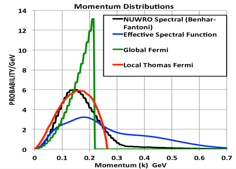
Figure 1: One-dimensional nucleon momentum distributions in a ${}_{6}^{12}$C nucleus. The green curve (Global Fermi) is the momentum distribution for the relativistic Fermi gas (RFG) model. The red curve is the Local-Thomas-Fermi (LTM) gas distribution. The black curve is the projected momentum distribution of the Benhar-Fantoni two dimensional spectral function. The blue line is the momentum distribution for the effective spectral function model, which approximates the $\psi^{\prime}$ superscaling prediction for the final state muon in quasielastic scattering.

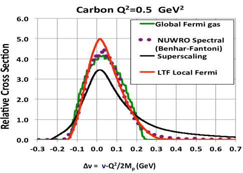
Figure 2: Comparison of the $\psi^{\prime}$ superscaling prediction (solid black line) for the normalized quasielastic $\frac{1}{\sigma}\frac{d\sigma}{d\nu}(Q^{2},\nu)$ at $Q^{2}$=0.5 GeV² for 10 GeV neutrinos on ${}_{6}^{12}$C to the predictions with several momentum distribution ($\nu=E_{0}-E^{\prime}$). Here the solid green curve labeled “Global Fermi” gas is the distribution for the Fermi gas model. The red line is the prediction for the local Thomas Fermi (LTF) gas, and the purple dots are the prediction using the two dimensional Benhar-Fantoni spectral function as implemented in nuwro.

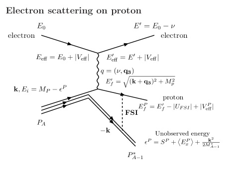
Figure 3: 1p1h process: Electron scattering from an off-shell bound proton of momentum $\vec{p_{i}}$=$\vec{k}$ in a nucleus of mass A. Here, the nucleon is moving in the mean field (MF) of all the other nucleons in the nucleus. The on-shell recoil excited $[A-1]^{*}$ spectator nucleus has a momentum $\vec{p}_{(A-1)*}=-\vec{k}$ and a mean excitation energy $\langle{E_{x}^{P}}\rangle$. The off-shell energy of the interacting nucleon is $E_{i}=M_{A}-\sqrt{(M_{A-1}*)^{2}+\vec{k}^{2}}=M_{A}-\sqrt{(M_{A-1}+{{E_{x}}})^{2}+\vec{k}^{2}}=M_{P}-\epsilon^{P}$, where $\epsilon^{P}=S^{P}+\langle E_{x}\rangle+\frac{\vec{k}^{2}}{2M^{*}_{A-1}}$. We model the effect of FSI (strong and EM interactions) by setting $E_{f}=\sqrt{(\vec{k}+\vec{q_{3}})^{2}+M_{P}^{2}}-|U_{FSI}|$+$|V_{eff}^{P}|$, where $U_{FSI}=U_{FSI}((\vec{q}_{3}+\vec{k})^{2})$. For electron QE scattering on bound protons $|V_{eff}^{P}|=\frac{Z}{Z-1}|V_{eff}|$, $E_{eff}=E_{0}+V_{eff}$, $E^{\prime}_{eff}=E^{\prime}+V_{eff}$.

${}_{Z}^{A}Nucl$	remove		remove
	proton	$S^{P}$	neutron	$S^{N}$	$S^{N+P}$
	Spectator		Spectator
${}_{1}^{2}$H	N	2.2	P	2.2	2.2
${}_{3}^{6}$Li 1+	${}_{2}^{5}$He $\frac{3}{2}$-	4.4	${}_{3}^{5}$Li $\frac{3}{2}$-	5.7	4.0
${}_{6}^{12}$C 0+	${}_{5}^{11}$B $\frac{3}{2}$-	16.0	${}_{6}^{11}$C $\frac{3}{2}$-	18.7	27.4
${}_{8}^{16}$O 0+	${}_{7}^{15}$N $\frac{1}{2}$-	12.1	${}_{8}^{15}$O $\frac{1}{2}$-	15.7	23.0
${}_{12}^{24}$Mg 0+	${}_{11}^{23}Na$ $\frac{3}{2}$+	11.7	${}_{12}^{23}$ Mg $\frac{3}{2}$+	16.5	24.1
${}_{13}^{27}$Al$\frac{5}{2}$+	${}_{12}^{26}Mg$ 0+	8.3	${}_{12}^{23}$ Al 5+	13.1	19.4
${}_{14}^{28}$Si 0+	${}_{13}^{27}$Al$\frac{5}{2}$+	11.6	${}_{14}^{27}$Si $\frac{5}{2}$+	17.2	24.7
${}_{18}^{40}$Ar$\frac{3}{2}$+	${}_{17}^{39}$CL $\frac{3}{2}$+	12.5	${}_{18}^{39}$Ar $\frac{7}{2}$-	9.9	20.6
${}_{20}^{40}$Ca 0+	${}_{19}^{39}$K $\frac{3}{2}$ +	8.3	${}_{20}^{39}$Ca $\frac{3}{2}$+	15.6	21.4
${}_{23}^{51}$V $\frac{7}{2}$-	${}_{22}^{50}$Ti 0+	8.1	${}_{23}^{50}$V 6+	11.1	19.0
${}_{26}^{56}$Fe 0+	${}_{25}^{55}$Mn $\frac{5}{2}$ -	10.2	${}_{26}^{55}$Fe $\frac{3}{2}$-	11.2	20.4
${}_{28}^{58}$Ni $\frac{3}{2}$ -	${}_{27}^{58}$Co 2+	8.2	${}_{87}^{58}$Ni 0+	12.2	19.5
${}_{39}^{89}$Y $\frac{1}{2}$ -	${}_{38}^{88}$Sr $\frac{1}{2}$-	7.1	${}_{39}^{88}$Y 4-	11.5	18.2
${}_{40}^{90}$Zr 0+	${}_{39}^{89}$Y $\frac{1}{2}$ -	8.4	${}_{40}^{88}$Zr$\frac{9}{2}$+	12.0	17.8
${}_{50}^{120}$Sn 0+	${}_{49}^{119}$In $\frac{9}{2}$ +	10.1	${}_{50}^{119}$Sn $\frac{1}{2}$+	8.5	17.3
${}_{73}^{181}$Ta$\frac{7}{2}$ -	${}_{72}^{180}$Hf 0+	5.9	${}_{73}^{180}$Ta 1+	7.6	13.5
${}_{79}^{197}$Au$\frac{3}{2}$+	${}_{78}^{196}$Pt 0+	5.8	${}_{79}^{196}$Au 2-	8.1	13.7
${}_{82}^{208}$Pb 0+	${}_{81}^{207}$TI $\frac{1}{2}$+	8.0	${}_{82}^{207}$Pb $\frac{1}{2}$-	7.4	14.9

Table 1: The spin parity transitions and separation energies $S^{P}$, $S^{N}$ and $S^{N+P}$ when a proton or a neutron or both are removed from various nuclei. All energies are in MeV.

2 The Impulse Approximation

2.1 1p1h process

Fig. 3 is a descriptive diagram for QE electron scattering on an off-shell proton which is bound in a nucleus of mass $M_{A}$, and is moving in the mean field (MF) of all other nucleons in the nucleus. The on-shell recoil excited $[A-1]^{*}$ spectator nucleus has a momentum $\vec{p}_{(A-1)*}=-\vec{k}$ and a mean excitation energy $\langle{E_{x}^{P}}\rangle$. The off-shell energy of the interacting nucleon is $E_{i}=M_{A}-\sqrt{(M_{A-1}*)^{2}+\vec{k}^{2}}=M_{A}-\sqrt{(M_{A-1}+{{E_{x}}})^{2}+\vec{k}^{2}}=M_{P}-\epsilon^{P}$, where $\epsilon^{P}=S^{P}+\langle E_{x}\rangle+\frac{\vec{k}^{2}}{2M^{*}_{A-1}}$. As discussed in section 4 we model the effect of FSI (strong and EM interactions) by setting $E_{f}=\sqrt{(\vec{k}+\vec{q_{3}})^{2}+M_{P}^{2}}-|U_{FSI}|$+$|V_{eff}^{P}|$, where $U_{FSI}=U_{FSI}((\vec{q}_{3}+\vec{k})^{2})$.

Table 1 shows the spin and parity of the initial state nucleus, and the spin parity of the ground state of the spectator nucleus when a bound proton or a bound neutron is removed via the 1p1h process.

The four-momentum transfer to the nuclear target is defined as $q=(\vec{q}_{3},\nu)$. Here $\vec{q}_{3}^{2}$ is the 3-momentum transfer, $\nu$ is the energy transfer, and $Q^{2}=-q^{2}=\vec{q}^{2}-\nu^{2}$ is the square of the four-momentum transfer. For QE electron scattering on unbound protons (or neutrons) the energy transfer $\nu$ is equal to $Q^{2}/2M_{P,N}$ where $M_{P}$ is mass of the proton and $M_{N}$ is the mass of the neutron, respectively.

2.2 Nuclear Density corrections to $k_{F}^{P}$ and $k_{F}^{N}$

The values of the Fermi momentum $k_{F}$ that are currently used in neutrino Monte Carlo generators are usually taken from an analysis of e-A data by Moniz et al.electron . The Moniz published values of $k_{F}$ were extracted using the RFG model under the assumption that the Fermi momenta for protons and neutrons are different and are related to $k_{F}$ via the relations $k_{F}^{N}=k_{F}(2N/A)^{1/3}$ and $k_{F}^{P}=k_{F}(2Z/A)^{1/3}$, respectively. What is actually measured is $k_{F}^{P}$, and what is published is $k_{F}$. Moniz assumes that the nuclear density (nucleons per unit volume) is constant. Therefore, in the same nuclear radius R, $k_{F}^{N}$ for neutrons is larger if N is greater than Z. Moniz used these expressions to extract the published value of $k_{F}$ from the measured value of $k_{F}^{P}$.

We undo this correction and re-extract the measured values of $k_{F}^{P}$ for nuclei which have a different number of neutrons and protons. In order to obtain the values of $k_{F}^{N}$ from the measured values of $k^{P}_{F}$ we use the fact that the Fermi momentum is proportional to the cube root of the nuclear density. Consequently $k_{F}^{N}=C\frac{N^{1/3}}{R_{N}}$, and $k_{F}^{P}=C\frac{Z^{1/3}}{R_{P}}$, and $k_{F}^{N}=k_{F}^{P}\frac{N^{1/3}R_{P}}{Z^{1/3}R_{N}}$. For the proton and neutron radii, we use the fits for the half density radii of nuclei (in units of femtometer) given in ref.radii .

$$R_{P} = 1.322Z^{1/3}+0.007N+0.022$$ (3)

$$R_{N} = 0.953N^{1/3}+0.015Z+0.774.$$ (4)

We only these fits for nuclei which do not have an equal number of protons and neutrons. For nuclei which have an equal number of neutrons and protons we assume that $k_{F}^{N}=k_{F}^{P}$=$k_{F}(Moniz)$.

However for the ${}_{82}^{208}$Pb nucleus only we use $k_{F}^{P}$=0.275 GeV which we obtain from our own fits to inclusive e-A scattering data. For all other nuclei, our values are consistent with the values extracted by Moniz et. al.

2.3 Separation energy

The separation energy for a proton ($S^{P}$) or neutron $S^{N}$ is defined as follows:

$$M_{A}=M_{A-1}+M_{N,P}-S^{N,P}$$ (5)

The energy to separate both a proton and neutron ($S^{P+N}$) is defined as follows:

$$M_{A}=M_{A-2}+M_{P}+M_{N}-S^{N+P}$$ (6)

The proton and neutron separation energies S^P and S^N are available in nuclear data tables. The values of S^P, S^N and $S^{N+P}$ for various nucleiTUNL ; nuclear-data are given in Table 1

2.4 Two nucleon correlations

Fig. 4 illustrates the 2p2h process originating from both long range and short range two nucleon correlations (src). Here the scattering is from an off-shell bound proton of momentum $\vec{p}_{i}$=$\vec{k}$. The momentum of the initial state off-shell interacting nucleon is balanced by a single on-shell correlated recoil neutron which has momentum $-\vec{k}$. The $[A-2]^{*}$ spectator nucleus is left with two holes. Short range nucleon-proton correlations occur $\approx 20$% of the timemiller . The off-shell energy of the interacting bound proton in a quasi-deuteron is $(E_{i}^{P})_{src}=M_{D}-\sqrt{M_{N}+{\vec{k}}^{2}}-S^{P+N}$, where $M_{D}$ is the mass of the deuteron. For QE scattering there is an additional 2p2h transverse cross section from “Meson Exchange Currents” (mec) and “Isobar Excitation” (ie).

In this paper we only focus on the extraction of the average removal energy parameters for 1p1h processes. Processes leading to 2p2h final states (src, mec and ie) result in larger missing energy and should be modeled separately.

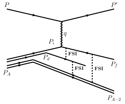
Figure 4: 2p2h process: Electron scattering from an off-shell bound proton of momentum $\vec{p}_{i}$=$\vec{k}$ from two nucleon short range correlations (quasi-deuteron). There is an on-shell spectator (A-2) * nucleus and an on-shell spectator recoil neutron with momentum $-\vec{k}$. The off-shell energy of the interacting bound proton is $E_{i}^{P}(src)=M_{D}-\sqrt{M_{N}+{\vec{k}}^{2}}-S^{P+N}$.

Symbol
	Spectator Nucleus Excitation
$E_{x}^{P,N}$	Used in spectral functions
	implemented in geniegenie
$S^{P,N}$	Separation Energy
= $M_{A-1}+M_{P,N}-M_{A}$	Nuclear Data Tables
	(measured) TUNL ; nuclear-data
	missing energy
$E_{m}^{P,N}$=$S^{P,N}$+$E_{x}^{P,N}$	used in spectral functions
	removal energy is $\epsilon^{P,N}$
${\epsilon^{P,N}}$=$E_{m}^{P,N}$+$T_{A-1}$	$E_{i}=M-{\epsilon^{P,N}}$
$T_{A-1}=$	used in $E_{\nu}^{QE-\mu}$, $Q^{2}_{QE-\mu}$,
$=\sqrt{\vec{k}^{2}+M_{A-1}^{2}}-M_{A-1}$	and $Q^{2}_{QE-P}$, also used in
$\approx\frac{\vec{k}^{2}}{2M_{A-1}}$	effective spectral functionseffective
$\epsilon_{SM}^{\prime(P,N)}$=${\epsilon^{P,N}}+T^{P,N}_{av}$	$\epsilon_{SM}^{\prime(P,N)}$ is Smith Monizneutrino
$T=\sqrt{\vec{k}^{2}+M^{2}}-M$	Interaction energy
	$E_{i}=M+T-\epsilon_{SM}^{\prime(P,N)}$
$\langle k^{2}\rangle=0.6k_{F}^{2}$	used in old-neutneut
$x^{\nu}$= $\epsilon^{N}-|U_{FSI}|$	we use $x^{\nu,\bar{\nu}}$ to include
$+|V_{eff}^{P}|$	the effects of FSI.
$x^{\bar{\nu}}$=$\epsilon^{P}-|U_{FSI}|$	$U_{FSI}=U_{FSI}((\vec{q}_{3}+\vec{k})^{2})$

Table 2: Summary of the relationships between excitation energy $E_{x}^{P,N}$ (used in genie), separation energy $S^{P,N}$, missing (missing) energy $E_{m}^{P,N}$ (used in spectral function measurements), removal energy ${\epsilon^{P,N}}$ (used in the reconstruction of neutrino energy from muon kinematics only), the Smith-Moniz removal energy $\epsilon_{SM}^{\prime P,N}$ (that should be used in old-neut) and the parameters $x$ and $x^{\nu,\bar{\nu}}(\vec{q}_{3}+\vec{k})^{2})$ which we use to include the effects of FSI in electron and neutrino/antineutrino scattering. For QE neutrino scattering on bound neutrons $|V_{eff}^{P}|=|V_{eff}|$

.

Target	Q2	$\langle T^{P}\rangle$	$\langle E_{m}^{P}\rangle$
		$E_{m}^{P}<80$	$E_{m}^{P}<80$
$\bf{}_{6}^{12}C$	0.6	15.9	26.0
Jlab Hall C C12	1.2	16.3	25.8
	1.8	16.0	26.6
	3.2	17.3	26.2
Jlab $\langle T^{P}\rangle^{SF}$, $\langle E_{m}^{P}\rangle^{SF}$	Ave.	16.4$\pm$0.6	26.1$\pm$0.4
Saclay $\langle T^{P}\rangle^{SF}$,$\langle E_{m}^{P}\rangle^{SF}$		16.9$\pm$0.5	23.4$\pm$0.5
Saclay $\langle E_{m}^{P}\rangle^{levels}$			24.4$\pm$2
$k_{F}^{P}$=221$\pm$5		15.5 $\pm$1.2
Target	Q2	$\langle T^{P}\rangle$	$\langle E_{m}^{P}\rangle$
$\bf{}_{14}^{28}Si$
Saclay $\langle T^{P}\rangle^{SF}$, $\langle E_{m}^{P}\rangle^{SF}$		17.0$\pm$0.6	24.0$\pm$0.6
Saclay $\langle E_{m}^{P}\rangle^{levels}$			27.6$\pm$2
$k_{F}^{P}$=239$\pm$5		18.1$\pm$1.3
Target	Q2	$\langle T^{P}\rangle$	$\langle E_{m}^{P}\rangle$
$\bf{}_{20}^{40}Ca$
Saclay $\langle T^{P}\rangle^{SF}$, $\langle E_{m}^{P}\rangle^{SF}$		16.6$\pm$0.5	27.8$\pm$0.5
Saclay$\langle E_{m}^{P}\rangle^{levels}$			26.5$\pm$2
$k_{F}^{P}$=239$\pm$5		18.1$\pm$1.3
Target	Q2	$\langle T^{P}\rangle$	$\langle E_{m}^{P}\rangle$
$\bf{}_{26}^{56}Fe$	0.6	20.4	30.7
Jlab Hall C C12	1.2	18.1	29.4
	1.8	17.8	27.8
	3.2	19.1	28.8
Jlab $\langle T^{P}\rangle^{SF}$, $\langle E_{m}^{P}\rangle^{SF}$	Ave.	18.8$\pm$1.0	29.2$\pm$1.1
$k_{F}^{P}$=254$\pm$5		20.4$\pm$1.4
Target	Q2	$\langle T^{P}\rangle$	$\langle E_{m}^{P}\rangle$
$\bf{}_{28}^{58}Ni$
Saclay $\langle T^{P}\rangle^{SF}$,$\langle E_{m}^{P}\rangle^{SF}$		18.8$\pm$0.7	25.0$\pm$0.7
Saclay$\langle E_{m}^{P}\rangle^{levels}$			25.3$\pm$2
$k_{F}^{P}$=257$\pm$5		20.9$\pm$1.4
Target	Q2	$\langle T^{P}\rangle$	$\langle E_{m}^{P}\rangle$
$\bf{}_{79}^{197}Au$	0.6	20.2	25.5
Jlab Hall C C12	1.2	18.4	25.7
	1.8	18.3	24.1
	3.2	19.4	26.1
Jlab $\langle T^{P}\rangle^{SF}$, $\langle E_{m}^{P}\rangle^{SF}$	Ave.	19.1$\pm$0.8	25.3$\pm$0.8
$k_{F}^{P}$=24.5$\pm$5		19.0$\pm$1.3

Table 3: Average values of the proton kinetic energy $\langle T^{P}\rangle^{SF}$ and missing energy $\langle E_{m}^{P}\rangle^{SF}$ for 1p1h final states ($E_{m}^{P}<80$) extracted from published tests of the Koltun sum rule using spectral function (SF) measurements at Jefferson lab Hall AC12 and SaclaySaclay . For a Fermi gas distribution $\langle T^{P}\rangle=\frac{3}{5}(k_{F}^{P})^{2}$ All energies are in MeV. The bolded numbers are the best estimates for each target.

3 Spectral functions and $ee^{\prime}p$ experiments

In $ee^{\prime}p$ experiments the following process is investigated:

$$e+A\to e^{\prime}+(A-1)^{\star}+p_{f}.$$ (7)

Here, an electron beam is incident on a nuclear target of mass $M_{A}$. The hadronic final state consists of a proton of four momentum $p_{f}\equiv(E_{f},{\vec{p}_{f}})$ and an undetected nuclear remnant $(A-1)^{\star}$. Both the final state electron and the final state proton are measured. The $(A-1)^{\star}$ nuclear remnant can be a $(A-1,Z-1)$ spectator nucleus with excitation $E_{x}^{P}$, or a nuclear remnant with additional unbound nucleons.

At high energies, within the plane wave impulse approximation (PWIA) the initial momentum $\vec{k}$ of the initial state off-shell interacting nucleon can be identified approximately with the missing momentum ${\vec{p}}_{m}$. Here we define $p_{m}$ = $|{\vec{p}}_{m}|$ and $k=|\vec{k}|$

$${\vec{p}}_{m}={\vec{p}_{f}}-{\vec{q}_{3}}\approx\vec{k}.$$ (8)

The missing energy $E_{m}$ is defined by the following relativistic energy conservation expression,

$$\nu+M_{A}=\sqrt{(M_{A-1}^{*})^{2}+\vec{p_{m}}^{2}}+E_{f}^{P}$$ (9)

$$E_{f}^{P}=\sqrt{{\vec{p}_{f}^{2}}+M_{P}^{2}},~{}~{}~{}~{}~{}M_{A-1}^{*}=M_{A}-M+E_{m}.$$

The missing energy $E_{m}$ can be expressed in term of the excitation energy ($E_{x}$) of the spectator (A-1) nucleus and the separation energy of the proton $S^{P}$ (or neutron $S^{N}$).

$$E_{m}^{P,N} = S^{P,N}+E_{x}^{P,N}$$ (10)

The probability distribution of finding a nucleon with initial state momentum $p_{m}\approx k$ and missing energy $E_{m}$ from the target nucleus is described by the spectral function, defined as $P_{SF}(p_{m},E_{m})$. Note that for spectral functions both $P(p_{m},E_{m})$ and $S(p_{m},E_{m})$ notation are used in some publications. The spectral functions $P_{SF}^{P}(p_{m},E_{m}^{P})$ and $P_{SF}^{N}({p_{m}},E_{m}^{N})$ for protons and neutrons are two dimensional distributions which can be measured (or calculated theoretically). Corrections for final state interactions of the outgoing nucleon are required in the extraction of $P_{SF}^{P}(p_{m},E_{m}^{P})$ from $ee^{\prime}p$ data. The kinematical region corresponding to low missing momentum and energy is where shell modelbrown states dominatereview . In practice, only the spectral function for protons can be measured reliably.

In addition to the 1p1h contribution in which the residual nucleus is left in the ground or excited bound state, the measured spectral function includes contributions from nucleon-nucleon correlations in the initial state (2p2h) where there is one or more additional spectator nucleons. Spectral function measurements cannot differentiate between a spectator (A-1) nucleus and a spectator (A-2) nucleus from src because the 2nd final state src spectator nucleon is not detected.

Here, we focus on the spectral function for the 1p1h process, which dominates for $E_{m}$ less than 80 MeV, and ignore the spectral function for the 2p2h process which dominates at higher values of $E_{m}$. We use shell model calculations to obtain the difference in the binding energy parameters for neutrons and protons.

Nucleus		${}_{6}^{12}C$					${}_{14}^{28}Si$		${}_{28}^{58}Ni$
$S^{P}$		16.0					11.6		8.2
		shell	shell	shell			shell		shell
ee′p		missing	missing	missing			missing		missing
$\epsilon^{P}$=$E_{m}$+$T_{A-1}$		energy	energy	energy	width		energy		energy
		$E_{m}^{P}$	$E_{m}^{P}$	$E_{m}^{P}$	fwhm		$E_{m}^{P}$		$E_{m}^{P}$
		Saclay	nikhef	Tokyo	Tokyo		Saclay		Saclay
1s1/2	2	38.1$\pm$1.0	42.6$\pm$5	36.9$\pm$0.3	19.8$\pm$0.5	2	51.0	2	62.0
1p3/2,1/2	4	17.5$\pm$0.4	17.3$\pm 0.4$	15.5$\pm 0.1$	6.9$\pm$0.1	6	32.0	6	45.0
1d5/2,3/2						4	16.1$\pm$0.8	10	21.0
2s1/2						2	13.8$\pm$0.5	2	14.7$\pm$0.2
1f7/2								8	9.3$\pm$0.3
$\langle E_{m}^{P}\rangle^{levels}$	6	$\bf{\langle 24.4\pm 2\rangle}$	$\bf{\langle 25.7\pm 2\rangle}$	$\bf{\langle 22.6\pm 3\rangle}$		14	$\bf{\langle 27.6\pm 2\rangle}$	28	$\bf{{\langle 25.3\pm 2\rangle}}$
$T_{A-1}$		1.4	1.4	1.4			0.7		0.4
$\langle\epsilon^{P}\rangle^{levels}$	6	$\bf{\langle 25.8\pm 2\rangle}$	$\bf{\langle 27.1\pm 2\rangle}$	$\bf{\langle 24.0\pm 3\rangle}$		14	$\bf{\langle 28.3\pm 2\rangle}$	28	$\bf{{\langle 25.7\pm 2\rangle}}$

Table 4: Results of a DPWA analysis of the “level missing energies” for different shell-model levels done by the SaclaySaclay and TokyoTokyo1 ; Tokyo2 ; Tokyo3 $ee^{\prime}p$ experiments on ${}_{6}^{12}C$, ${}_{14}^{28}Si$ and ${}_{28}^{58}Ni$.

Nucleus		${}_{3}^{6}Li$		${}_{13}^{27}Al$		${}_{20}^{40}Ca$				${}_{23}^{51}V$
$S^{p}$		4.4		8.3		8.3				8.1
		Shell		Shell		Shell	Shell			Shell
ee′p		missing		missing		missing	missing			missing
$\epsilon^{P}$=		energy		energy		energy	energy	width		energy	width
$E_{m}$+$T_{A-1}$		$E_{m}^{P}$		$E_{m}^{P}$		$E_{m}^{P}$	$E_{m}^{P}$	fwhm		$E_{m}^{P}$	fwhm
		Tokyo		Tokyo		Saclay	Tokyo	Tokyo		Tokyo	Tokyo
1s1/2	2	22.6$\pm$0.2	2	57$\pm$3	2	56.0	59$\pm$3	34$\pm$10	2	60$\pm$3	36$\pm$ 11
1p3/2,1/2	1	4.5$\pm$0.2	6	34$\pm$1	6	41.0	35$\pm$1	21$\pm$3	6	40$\pm$1	25$\pm$4
1d5/2			4	14.0$\pm$0.6	6	*14.9$\pm$0.8	19.0$\pm$1.1	10$\pm$3	6	19.5$\pm$0.5	19$\pm$2
2s1/2			1	14.3$\pm$0.2	2	11.2$\pm$0.3	14.4$\pm$0.3	13$\pm$1	2	15.1$\pm$0.2	5$\pm$2
1d3/2					4	*14.9$\pm$0.8	10.9$\pm$0.7	9$\pm$1
1f7/2						*combined			7	10.3$\pm$1.1	5$\pm$3
${\langle E_{m}^{P}\rangle}^{levels}$	3	$\bf{\langle 16.6\pm 2\rangle}$	13	$\bf{\langle 29.9\pm 3\rangle}$	20	$\bf{\langle 26.5\pm 3\rangle}$	$\bf{\langle 25.7\pm 3\rangle}$		23	$\bf{\langle 25.2\pm 3\rangle}$
$T_{A-1}$		1.8		0.7		0.5	0.5			0.4
${\bf\langle\epsilon^{P}\rangle}^{levels}$	3	$\bf{\langle 18.4\pm 2\rangle}$	13	$\bf{\langle 30.6\pm 3\rangle}$	20	$\bf{\langle 27.0\pm 3\rangle}$	$\bf{\langle 26.3\pm 3\rangle}$		23	$\bf{\langle 25.6\pm 3\rangle}$

Table 5: Results of a DPWA analysis of the “level missing energies” for different shell-model levels done by the SaclaySaclay and TokyoTokyo1 ; Tokyo2 ; Tokyo3 $ee^{\prime}p$ experiments on on ${}_{3}^{6}Li$, ${}_{13}^{27}Al$, ${}_{20}^{40}Ca$ and ${}_{23}^{51}V$.

4 Effects of the optical and Coulomb potentials (FSI)

We use empirical parameter $U_{FSI}((\vec{q}_{3}+\vec{k})^{2})$ to approximate the effect of the interaction of the final state proton with the optical potential of the spectator nucleus. This is important at low values of $\vec{q}_{3}^{2}$. In addition, we include the effect of the interaction of the final state proton with the Coulomb field of the nucleus ($V_{eff}^{P}$).

In QE scattering of electrons a three momentum transfer $\vec{q}_{3}$ to a bound proton with initial momentum $\vec{k}$ results in the following energy $E_{f}^{P}$ of the final state proton:

$$E_{f}^{P} = \sqrt{{\vec{(}k+\vec{q}_{3})^{2}}+M_{P}^{2}}-|U_{FSI}((\vec{q}_{3}+\vec{k})^{2})|+|V_{eff}^{P}|$$

where for electron scattering on bound protons $V_{eff}^{P}=\frac{Z-1}{Z}|V_{eff}|$. The Coulomb correction $|V_{eff}|$ is discussed in Appendix A.

We define the average removal energy $\epsilon^{P,N}$ in terms of the average momentum $\langle k^{2}\rangle^{P,N}$ of the bound nucleon as follows:

$$\epsilon^{P,N} = E_{m}^{P,N}+T^{N,P}_{A-1}$$

$$= S^{P,N}+E_{x}^{P,N}+\frac{\langle k^{2}\rangle^{P,N}}{2M^{*}_{A-1}}$$

In order to properly simulate neutrino interactions we extract values of the average missing energy (or equivalently the average excitation energy) from spectral functions measured in ee^′p experiments. We then use these values and extract $U_{FSI}((\vec{q}_{3}+\vec{k})^{2})$ from inclusive e-A as discussed in section 9.

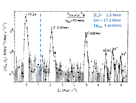
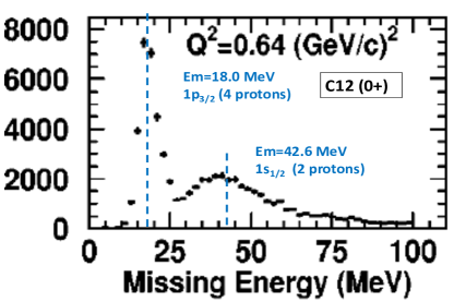
Figure 5: Top panel: The measuredhuberts NIKHEF high resolution spectral function for protons in the 1p level of ${}_{6}^{12}C$ as a function of the spectator nucleus excitation energy $E_{x}^{P}$ for ${\vec{p}_{m}}=\vec{k}$ = 172 MeV/c. Bottom panel: The Jlab measurementC12 of the one-dimensional spectral function for ${}_{6}^{12}C$ as a function of missing energy $E_{m}^{P}$ for $Q^{2}$= 0.64 GeV².

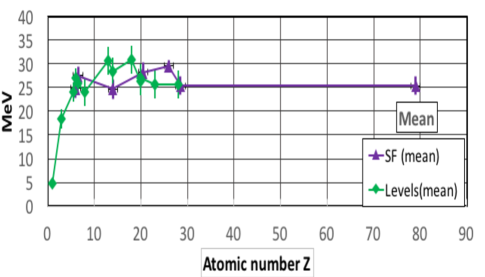
Figure 6: Average removal energies versus atomic number Z. Values of $\langle\epsilon^{P}\rangle^{SF}$ from tests of the Koltun sum rule in $ee^{\prime}p$ experiments (in purple) are compared to values of $\langle\epsilon^{P}\rangle^{levels}$ extracted from $ee^{\prime}p$ measurements of “level missing energies” (in green).

	${\bf{}^{12}_{6}C}$	proton	neutron	N-P	${\bf{}^{16}_{8}O}$	proton	proton	neutron	N-P
$T_{A-1}$		1.4	1.4	Diff		1.1	1.1	1.1	Diff
		binding	binding			Jlab shell	binding	binding
		energy	energy			missing energy	energy	energy
$S^{P}$,$S^{N}$		16.0	18.7	2.7		12.1	12.1	15.7	3.6
1s1/2	2	42.6	43.9	1.3	2	42$\pm$2	45.0	47.0	2.0
							( 40$\pm$8)
1p3/2	4	16.0	18.7	2.7	4	18.9$\pm$0.5	18.4	21.8	3.4
1p1/2					2	12.1$\pm$0.5	12.1	15.7	3.6
$average~{}\langle E_{m}^{P}\rangle,BE$	6	$\langle 24.9\rangle$	$\langle 27.1\rangle$	2.6	8	$\langle{23.0\pm 2}\rangle$	$\langle 23.5\rangle$	$\langle 26.6\rangle$	$\bf 2.9\pm 1$

Table 6: Shell-model single particle binding energies for ${}^{12}_{8}C$ and ${}^{16}_{8}O$ from ref.spectral-theory . When available, the experimental values shown in italics are used. The difference between the average missing energies $\langle E_{m}^{P,N}\rangle$ for neutrons and protons can be approximated by the difference in the weighted average of the single particle binding energies of all shell-model levels. We obtain N-P differences of 2.6 and 2.9 MeV for ${}^{12}_{8}C$ and ${}^{16}_{8}O$, respectively. These differences are close to the corresponding differences in separation energies of neutrons and protons ($S^{N}$-$S^{P}$) of 2.7 and 3.6 MeV, for ${}^{12}_{8}C$ and ${}^{16}_{8}O$, respectively.

4.1 Smith-Moniz formalism

The Smith-Monizneutrino formalism uses on-shell description of the initial state. In the on-shell formalism, the energy conserving expression is

$$\nu+M-\epsilon=E_{f}$$

is replaced with

$$\nu+\sqrt{k^{2}+M^{2}}-\epsilon_{SM}^{\prime P,N}=E_{f}.$$

Therefore,

$$\epsilon_{SM}^{\prime}=\epsilon+\langle T^{P,N}\rangle,$$

where

$$\langle T^{P,N}\rangle=\sqrt{\langle k^{2}\rangle^{P,N}+M^{2}}-M\approx\frac{3}{5}\frac{(k_{F}^{P,N})^{2}}{2M}$$

A summary of the relationships between excitation energy $E_{x}^{P,N}$ used in genie (which incorporates the Bodek-Ritchie BodekRitchie off-shell formalism), separation energy $S^{P,N}$, missing missing energy $E_{m}^{P,N}$ (used in spectral function measurements), removal energy ${\epsilon^{P,N}}$ (used in the reconstruction of neutrino energy from muon kinematics only) and the Smith-Moniz removal energy $\epsilon_{SM}^{\prime P,N}$ (that should be used in old-neut) is given in Table 2.

5 Extraction of average missing energy $\langle E_{m}\rangle$

We extract the average missing energy ${\langle E_{m}^{P}\rangle}$ and excitation energy ${\langle E_{x}^{P}\rangle}$ for the 1p1h process from $ee^{\prime}P$ electron scattering data using two methods.

1. $\langle E_{m}^{P}\rangle^{SF}$: From direct measurements of the average missing energy ${\langle E_{m}^{P}\rangle}$ and average proton kinetic energy ${\langle T^{P}\rangle}$. These quantities have been extracted from spectral functions measured in ee^′p experiments for tests of the Koltun sum ruleKoltun . The contribution of two nucleon corrections is minimized by restricting the analysis to $E_{m}^{P}<$ 80 MeV. This is the most reliable determination of $\langle E_{m}^{P}\rangle$. We refer to this average as $\langle E_{m}^{P}\rangle^{SF}.$              

2. $\langle E_{m}^{P}\rangle^{levels}$: By taking the average (weighted by shell model number of nucleons) of the nucleon “level missing energies” of all shell model levels which are extracted from spectral functions measured in ee^′p experiments. We refer to this average as $\langle E_{m}^{P}\rangle^{levels}.$

There could be bias in method 2 originating from the fact that a fraction of the nucleons ($\approx 20\%$) in each level are in a correlated state with other nucleons (leading to 2p2h final states). The fraction of correlated nucleons is not necessarily the same for all shell-model levels. As discussed in section 5.4 (and shown Fig. 6)we find that the values of $\langle E_{m}^{P}\rangle^{levels}$ are consistent with $\langle E_{m}^{P}\rangle^{SF}$ for nuclei for which both are available.

When available, we extract the removal energy parameters using $\langle E_{m}^{P}\rangle^{SF}$ from method 1. Otherwise we use $\langle E_{m}^{P}\rangle^{levels}$ from method 2. For each of the two methods, we also use the nuclear shell model to estimate difference between the missing energies for neutrons and protons.

		$k_{F}^{P}$,$k_{F}^{N}$	$k_{F}^{P}$	$E_{\mathrm{shift}}$	$|V_{eff|}$		${{\epsilon}}^{P}$ (MeV)
	${}_{Z}^{A}Nucl$	Moniz	$\psi^{\prime}$ fit	$\psi^{\prime}$ fit	Gueye
	Nucl.	$\pm$5	ref.Donnelly	ref.Donnelly	ref.gueye
Source		updated
Source		MeV/c	MeV/c	MeV	MeV
	${}_{1}^{2}H$	88,88					*4.7$\pm$1
ee′p TokyoTokyo1 ; Tokyo2 ; Tokyo3	${}_{3}^{6}Li$	169,169	165	15.1	1.4	$\epsilon^{levels}$	*18.4$\pm$3
ee′p TokyoTokyo1 ; Tokyo2 ; Tokyo3	${{}_{6}^{12}C}$	221,221	228	20.0	3.1$\pm$0.25	$\epsilon^{levels}$	24.0$\pm$3
ee′p NIKHEFNIKHEFC12	${{}_{6}^{12}C}$					$\epsilon^{levels}$	27.1$\pm$3
ee′p SaclaySaclay	${{}_{6}^{12}C}$					$\epsilon^{levels}$	25.8$\pm$3
						$\langle\epsilon\rangle^{SF}$	24.8$\pm$3.0
Shell Model binding E	${{}_{6}^{12}C}$					$\epsilon_{shell-model}^{levels}$	24.9 $\pm$5
ee′p Jlab Hall C C12	${{}_{6}^{12}C}$					$\langle\epsilon\rangle^{SF}$	*27.5$\pm$3
ee′p Jlab Hall A O16	${{}_{8}^{16}O}$	225,225			3.4	$\epsilon^{levels}$	*24.1$\pm$3
Shell Model binding E	${{}_{8}^{16}O}$					$\epsilon_{shell-model}^{levels}$	23.5$\pm$5
ee′p TokyoTokyo1 ; Tokyo2 ; Tokyo3	${}_{13}^{27}Al$	238,241	236	18.0	5.1	$\epsilon^{levels}$	30.6 $\pm$3
ee′p SaclaySaclay	${}_{14}^{28}Si$	239,241			5.5	$\epsilon^{levels}$	28.3$\pm$2
						$\langle\epsilon\rangle^{SF}$	*24.7$\pm$3
${{}_{20}^{40}Ca}\rightarrow{{}_{18}^{40}Ar}$ Shell Model	${{}_{18}^{40}Ar}$	251,263			6.3	$\epsilon^{levels}$	*30.9$\pm$4
ee′p TokyoTokyo1 ; Tokyo2 ; Tokyo3	${{}_{20}^{40}Ca}$	251,251	241	28.8	7.4$\pm$0.6	$\Delta^{levels}$	26.3$\pm$3
ee′p SaclaySaclay	${{}_{20}^{40}Ca}$					$\epsilon^{levels}$	27.0$\pm$3
						$\langle\epsilon\rangle^{SF}$	*28.2$\pm$3
Shell-model binding E	${{}_{20}^{40}Ca}$					$\epsilon_{shell-model}^{levels}$	23.6$\pm$5
ee′p TokyoTokyo1 ; Tokyo2 ; Tokyo3	${}_{23}^{50}V$	253,266			8.1	$\epsilon^{levels}$	*25.6$\pm$3
ee′p Jlab hall C C12	${}_{26}^{56}Fe$	254,268	241	23.0	8.9$\pm$0.7	$\langle\epsilon\rangle^{SF}$	*29.6$\pm$3
ee′p SaclaySaclay	${}_{28}^{58.7}Ni$	257,269	245	30.0	9.8	$\epsilon^{levels}$	25.7$\pm$3
						$\langle\epsilon\rangle^{SF}$	*25.4$\pm$3
Shell-model binding E	${}_{40}^{88}Zr$				11.9$\pm$0.9	$\epsilon_{shell-model}^{levels}$	25.1$\pm$5
ee′p Jlab Hall C C12	${}_{79}^{197}Au$	275,311	245	25.0	18.5	$\langle\epsilon\rangle^{SF}$	*25.4$\pm$3
Shell Model binding E	${}_{82}^{208}Pb$	275,311	248	31.0	18.9$\pm$1.5	$\epsilon_{shell-model}^{levels}$	22.8$\pm$5

Table 7: Comparison of removal energies $\langle\epsilon\rangle^{SF}$ from tests of the Koltun sum rule (by SaclaySaclay , and Jlab Hall C C12 ) to $\langle\epsilon^{P}\rangle^{levels}$ extracted from the missing energies of shell-model levels measured in $ee^{\prime}p$ experiments by TokyoTokyo1 ; Tokyo2 ; Tokyo3 , SaclaySaclay , Jlab Hall AO16 , Jlab Hall C C12 , and nikhefNIKHEFC12 . In addition we show $\langle\epsilon^{P}\rangle^{levels}$ estimated from shell-model binding energies. The value in *bold is the best measurement for each nucleus.

5.1 Direct measurements of ${\langle E_{m}^{P}\rangle^{SF}}$ and ${\langle T^{P}\rangle^{SF}}$

The best estimates of the average missing energy ${\langle E_{m}^{P}\rangle}$ and average nucleon kinetic energy ${\langle T^{P}\rangle}$ are those that are directly extracted from spectral function measurements in analyses that test the Koltun sum rule Koltun . The Koltun’s sum rule states that

$$\frac{E_{B}}{A}=\frac{1}{2}\,[\,{\langle T^{P}\rangle^{SF}}\frac{A-2}{A-1}-{\langle E_{m}^{P}\rangle^{SF}}],$$ (12)

where $E_{B}/A$ is the nuclear binding energy per particle obtained from nuclear masses and includes a (small) correction for the Coulomb energy,

$${\langle T^{P}\rangle^{SF}}=\int d^{3}k~{}dE_{m}\ \frac{\vec{k}^{2}}{2M}P_{SF}(k,E_{m})\ ,$$ (13)

and

$${\langle E_{m}\rangle^{SF}}=\int d^{3}k~{}dE_{m}\ E_{m}\ P_{SF}(k,E_{m})\ .$$ (14)

For precise tests of the Koltun sum rule a small contribution from three-nucleon processes should be taken into account.

Values of $\langle E_{m}^{P}\rangle^{SF}$ and ${\langle T^{P}\rangle^{SF}}$ for the 1p1h process ($E_{m}^{P}<$80 MeV) published by Jlab Hall C experimentsC12 and by the Saclay groupSaclay are given in Table 3.

5.2 Spectral function “level missing energies”

Measured 2D spectral functions can be analyzed within the distorted plane wave approximation (DPWA) to extract the peak and width of the missing energy distribution $E_{m}^{P}$ for protons for each shell model level. We refer to it as the “level missing energy”. In some publications it is referred to as the “shell separation energy”. The energies and widths of the “level missing energies” for ${}_{3}^{6}Li$, ${}_{6}^{12}C$, ${}_{3}^{17}Al$, ${}_{20}^{40}Ca$, ${}_{23}^{50}V,$ extracted from data published by the Tokyo groupTokyo1 ; Tokyo2 ; Tokyo3 are shown in Tables 4 and 5. Also shown are the “level missing energies” for ${}_{6}^{12}C$, ${}_{14}^{28}Si$, ${}_{20}^{40}Ca$, and ${}_{28}^{58.7}Ni$, extracted from the data published by the SaclaySaclay group.

We obtain an estimate of the average missing energy $\langle E_{m}^{P}\rangle^{levels}$ for the 1p1h process by taking the average (weighted by the number of nucleons) of the “level missing energies” of all shell model levels with $E_{m}^{P}<$80 MeV. The results of our analysis of the Saclay and Tokyo data are given in Tables 4 and 5. As shown in Tables 4 and 5 for the deeply bound 1s and 1p levels in heavy nuclei the averages and widths of the missing energy distributions are large.

5.3 ${}_{6}^{12}C$ spectral function

The measuredhuberts ; NIKHEFC12 NIKHEF high resolution spectral function for the missing energy of a bound proton in the 1p level of ${}_{6}^{12}C$ as a function of the spectator nucleus excitation energy $E_{x}^{P}$ for ${\vec{p}_{m}}=\vec{k}$ = 172 MeV/c is shown in the top panel of Fig. 5. The Jlab measurementC12 of the one-dimensional spectral function for the missing energy for bound proton from ${}_{6}^{12}C$ as a function of $E_{m}^{P}$ for $Q^{2}$= 0.64 GeV² is shown in the bottom panel of of Fig. 5. The second peak at an average value of $E_{m}^{P}$ $\approx$ 42.6$\pm$5 MeV is for protons in the 1s level. Combining the two results (weighted by the number of nucleons in each level) we obtain $\langle E_{m}^{P}\rangle^{levels}$=25.7 $\pm$2 MeV for ${}_{6}^{12}C$. Additional details are given in Table 4.

			${\langle\epsilon^{P,N}\rangle}$	$\langle\epsilon^{\prime P,N}_{SM}\rangle$		$\Delta S$	$\langle E_{x}^{P,N}\rangle$		$\Delta E_{m}$
${}_{Z}^{A}N$	$\langle T^{P,N}\rangle$	$T_{A-1}^{P,N}$	Removal	smith-		N-P	bodek-	$\langle E_{m}^{P,N}\rangle$	N-P
	average	average	energy	moniz			ritchie	average
			$E_{m}$+$T_{A-1}^{P,N}$	${\epsilon^{P,N}}$+$T$			$E_{m}^{P,N}$-$S^{P,N}$
			use for	$\bf{old}$
		A-1	$E_{\nu}^{QE-\mu}$	$\bf{NEUT}$			$\bf{GENIE}$
	nucleon	nucleus	$Q^{2}_{QE-\mu}$	removal			excitation
	$\langle KE\rangle$	$\langle KE\rangle$	$Q^{2}_{QE-P}$	energy			energy		diff
	$T^{P}$,$T^{N}$	P, N	${\langle\epsilon^{P}\rangle}$,${\langle\epsilon^{N}\rangle}$	$\langle\epsilon^{\prime P}_{SM}\rangle$,$\langle\epsilon^{\prime N}_{SM}\rangle$	$S^{P}$, $S^{N}$	$diff$	$\langle E_{x}^{P}\rangle$,$\langle E_{x}^{N}\rangle$	$E_{m}^{P}$, $E_{m}^{N}$	$E_{m}^{N}$-$E_{m}^{P}$
$(_{1}^{2}H)$	2.5, 2.5	2.5, 2.5	4.7, 4.7	7.2, 7.2	2.2, 2.2	0.0	0.0, 0.0	2.2, 2.2	0.0
${}_{3}^{6}Li$	9.1, 9.1	1.8, 1.8	18.4, 19.7	27.5, 28.8	4.4, 5.7	1.3	12.2, 12.2	16.6, 17.9	(1.3)
${{}_{6}^{12}C}$	15.5, 15.5	1.4, 1.4	27.5, 30.1	43.0, 45.6	16.0, 18.7	2.7	10.1, 10.0	26.1, 28.7	2.6
${{}_{8}^{16}O}$	16.0, 16.0	1.1, 1.1	24.1, 27.0	40.1, 43.0	12.1, 15.7	3.6	10.9, 10.2	23.0, 25.9	2.9
${}_{13}^{27}Al$	17.9, 18.4	0.7, 0.7	30.6, 35.4	48.5, 53.3	8.3, 13.1	4.8	21.6, 21.6	29.9, 34.7	(4.8)
${}_{14}^{28}Si$	18.1, 18.4	0.7, 0.7	24.7, 30.3	42.8, 48.4	11.6, 17.2	5.6	12.4, 12.4	24.0, 29.6	(5.6)
${{}_{18}^{40}Ar}$	19.9, 21.9	0.5, 0.6	30.9, 32.3	50.8, 52.2	12.5, 9.9	-2.6	17.8, 21.8	30.2, 31.7	1.4
${{}_{20}^{40}Ca}$	19.9,19.9	0.5, 0.5	28.2, 35.9	48.1, 55.8	8.3, 15.6	7.3	19.4, 19.8	27.7, 35.4	7.7
${}_{23}^{50}V$	20.2, 22.4	0.4, 0.5	25.6, 28.6	45.8, 48.8	8.1, 11.1	3.0	17.0, 17.0	25.1, 28.1	(3.0)
${{}_{26}^{56}Fe}$	20.4, 22.6	0.4, 0.4	29.6, 30.6	50.0, 51.0	10.2, 11.2	1.0	19.0, 19.0	29.2, 30.2	(1.0)
${}_{28}^{58.7}Ni$	20.9, 22.8	0.4, 0.4	25.4, 29.4	46.3, 50.3	8.2, 12.2	4.0	16.8, 16.8	25.0, 29.0	(4.0)
${}_{40}^{88}Zr$					8.4, 12.0	3.6			1.9
${{}_{79}^{197}Au}$	23.9, 30.4	0.1, 0.1	25.4, 27.7	49.3, 57.6	5.8, 8.1	2.3	19.5, 19.5	25.3, 27.6	(2.3)
${}_{82}^{208}Pb$	23.9, 30.4	0.1, 0.1	22.8, 25.0	46.7, 55.4	8.0, 7.4	-0.6	14.7, 16.9	22.7, 24.9	2.2

Table 8: Summary of the parameters that enter into the extractions of excitation $\langle E_{m}^{P,N}\rangle$, removal energies $\langle\epsilon^{P,N}\rangle$, and the Smith-Moniz removal energy $\langle\epsilon^{\prime N}_{SM}\rangle$. All values are in MeV.

5.4 Comparison of the two methods

Tests of the Koltun sum rule as a function of $Q^{2}$ were done by $ee^{\prime}p$ experiments at Jlab Hall CC12 for ${}_{6}^{12}C$, ${}_{26}^{56}Fe$, and ${}_{79}^{197}Au$. Tests of the Koltun sum rule were also reported by the SaclaySaclay group for ${}_{6}^{12}C$, ${}_{14}^{28}Si$, ${}_{20}^{40}Ca$, and ${}_{28}^{59}Ni$. For both groups values of $\langle E_{m}^{P}\rangle^{SF}$ and $\langle T^{P}\rangle^{SF}$ were extracted from the measured spectral functions. The results from both groups are summarized in Table 3. We take the RMS variation with $Q^{2}$ of the Jefferson Lab Hall C data shown in Table 3 ($\approx$ 0.5 MeV) as the random error in the Jlab Hall C measurements of $\langle E_{m}^{P}\rangle^{SF}$.

We use the 2.7 MeV difference in the measured values of $\langle E_{m}^{P}\rangle^{SF}$ for ${}_{6}^{12}C$ at Jefferson Lab (26.1$\pm$0.4) and Saclay (23.4$\pm$0.5) as the systematic error in measurements of $\langle E_{m}^{P}\rangle^{SF}$. Since $\langle E_{m}^{P}\rangle^{SF}$ is the most reliable measurement of $\langle E_{m}^{P}\rangle$, we assign $\pm$3 MeV as the systematic uncertainty to all measurements of $\langle E_{m}^{P}\rangle$.

The average values of the removal energies $\langle\epsilon^{P}\rangle^{SF}$ = $\langle E_{m}^{P}\rangle^{SF}$ +$T_{A-1}$ versus atomic number from tests of the Koltun sum rule are in agreement with the average values extracted from measurements of “level missing energies” $\langle\epsilon^{P}\rangle^{levels}$= $\langle E_{m}^{P}\rangle^{levels}$ +$T_{A-1}$ as shown Fig. 6. For example, for the Saclay data shown in Table 3 the average of the difference between $\langle E_{m}^{P}\rangle^{levels}$ and $\langle E_{m}^{P}\rangle^{SF}$ for ${}_{6}^{12}C$, ${}_{14}^{28}Si$, ${}_{20}^{40}Ca$, and ${}_{28}^{59}Ni$ is 0.9$\pm$1.0 MeV.

5.5 Spectral function measurement of ${}_{8}^{16}O$

The spectral function for ${}_{8}^{16}O$ as a function of $E_{m}^{P}$ for ${\vec{p}_{m}}=\vec{k}$ = 60 MeV/c measured in Jlab Hall AO16 with 2.4 GeV incident electrons is shown in the top panel of Fig. 7. From this figure we extract a average $\langle E_{m}^{P}\rangle^{levels}$ = 23.0$\pm$2 MeV. Using $T_{A-1}$= 1.1 MeV for ${}_{8}^{16}O$ we also obtain a average $\langle\epsilon^{P}\rangle^{levels}$ = 24.1$\pm$2 MeV.

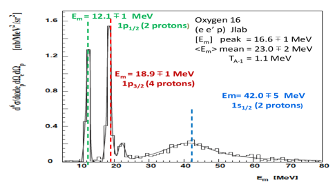
Figure 7: The spectral function for ${}_{8}^{16}O$ as a function of $E_{m}^{P}$ for ${\vec{p}_{m}}=\vec{k}$ = 60 MeV/c measured in Jlab Hall AO16 with 2.4 GeV incident electrons.

5.6 Difference between neutrons and protons for ${}^{12}_{8}C$ and ${}^{16}_{8}O$

For nuclei which have the same number of neutrons and protons we expect that the average excitation energy $E_{x}^{P,N}$ spectrum for protons and neutrons to be approximately the same ($\langle E_{x}^{P,N}\rangle\approx\langle E_{x}^{P,N}\rangle$). Since $E_{m}^{P,N}$=$S^{P,N}$+$E_{x}^{P,N}$ the difference in the average missing energies for neutrons and protons is approximately equal to the difference in separation energies $S^{N}-S^{P}$. By definition, the single particle binding energy of the least bound state is equal to the separation energy. The differences in the separation energies between neutrons and protons (S^N-S^P) bound in ${}^{12}_{8}C$ and ${}^{16}_{8}O$ are of 2.7 MeV and 3.6 MeV, respectively.

More generally, a better estimate of the difference between the average missing energies for neutrons and protons can be obtained from the nuclear shell model. The single nucleon missing energy $(E_{m}^{P,N})^{shell{\text{-}}model{\text{-}}level}$ for a nucleon in a given shell-model level is close (somewhat larger) to the single nucleon binding energy for that level. Consequently, the difference in the average missing energies for neutrons and protons for a nucleus $\langle E_{m}^{P}\rangle$-$\langle E_{m}^{N}\rangle$ is also approximately equal to the difference in the average binding energies.

The binding energies of different shell-model levelsspectral-theory for ${}^{12}_{8}C$ and ${}^{16}_{8}O$ are shown in Table 6. When available, the experimental values shown in italics are used. The differences between the averages of the nucleon binding energies in all shell-model levels for neutrons and protons is 2.6 and 2.9 MeV for ${}^{12}_{8}C$ and ${}^{16}_{8}O$, respectively. As expected these values are similar (within 1 MeV) to the differences in the separation energies for neutrons and protons (S^N-S^P) bound in ${}^{12}_{8}C$ and ${}^{16}_{8}O$ of of 2.7 and 3.6 MeV, respectively.

6 Inclusive e-A electron scattering

For QE $electron$ scattering at low $(\vec{k}+\vec{q}_{3})^{2}$ we use an empirical parameter $U_{FSI}((\vec{k}+\vec{q}_{3})^{2})$ to account for the effect of final state interactions. The off-shell Bodek-Ritchie formalism (used by genie) for the case of QE $electron$ scattering from a bound $proton$, should be implemented as follows:

$$\nu + (M_{P}-\epsilon^{P})=\sqrt{{\bf(k+\vec{q}_{3})^{2}}+M_{P}^{2}}-|U_{FSI}|+|V_{eff}^{P}|$$

$$\epsilon^{P} = S^{P}+\langle E_{x}^{P}\rangle+\frac{\langle\vec{k}^{2}\rangle}{2M_{A-1}^{*}}$$

$$\nu + (M_{P}-x^{P})=\sqrt{{\bf(k+\vec{q}_{3})^{2}}+M_{P}^{2}}$$

$$x^{P} = S^{P}+\langle E_{x}^{P}\rangle+\frac{\langle k^{2}\rangle}{2M_{A-1}}-|U_{FSI}|+|V_{eff}^{P}|$$

$$x^{N}=S^{N}+\langle E_{x}^{N}\rangle+\frac{\langle k^{2}\rangle}{2M_{A-1}}-|U_{FSI}|$$

$$Q^{2} = 4(E_{0}+|V_{eff}|)(E^{\prime}+|V_{eff})|\sin^{2}(\theta/2)$$

$$E^{\prime} = E_{0}-\nu,~{}~{}~{}~{}~{}E_{f}^{P}=\nu-\epsilon^{P},~{}~{}~{}~{}\vec{q}_{3}^{2}=Q^{2}+\nu^{2},$$ (15)

and $U_{FSI}=U_{FSI}((\vec{q}_{3}+\vec{k})^{2})$. For $electron$ scattering from a bound $proton$ $|V_{eff}^{P}|=\frac{Z-1}{Z}|V_{eff}|$, where (Z-1) is the number of protons in the spectator final state nucleus.

6.1 Smith-Moniz on-shell formalism

For QE $electron$ scattering on a bound proton in the Smith-Moniz on-shell formalism (used by old-neut) the following equations should be used:

$$\nu + M_{P}+T^{P}-\epsilon_{SM}^{\prime P}=$$

$$\sqrt{{\vec{(}k+\vec{q}_{3})^{2}}+M_{P}^{2}}-|U_{FSI}|+|V_{eff}^{P}|$$

$$T^{P} = \sqrt{\vec{k}^{2}+M^{2}_{P}}~{}~{}~{}~{}~{}~{}\epsilon^{P}=\epsilon_{SM}^{\prime P}-\langle T^{P}\rangle$$

$$\nu + [(M_{P}+T^{P})-x^{SM})]=\sqrt{{\bf(k+\vec{q}_{3})^{2}}+M_{P}^{2}}$$

$$x^{SM} = \epsilon_{SM}^{\prime P}-|U_{FSI}|+|V_{eff}^{P}|$$

$$Q^{2} = 4(E_{0}+|V_{eff}|)(E^{\prime}+|V_{eff}|)\sin^{2}(\theta/2)$$

$$E^{\prime} = E_{0}-\nu,~{}~{}~{}~{}E_{f}^{P}=\nu-\epsilon^{P},~{}~{}~{}~{}~{}\vec{q}_{3}^{2}=Q^{2}+\nu^{2},$$

and $U_{FSI}=U_{FSI}((\vec{q}_{3}+\vec{k})^{2})$.

6.2 Extraction of $U_{FSI}$ from in inclusive e-A QE data

We define $k_{z}$ as the component of k along the direction of the of the 3-momentum transfer $\vec{q}_{3}$.

$$\nu+(M_{P}-\epsilon^{P}) = \sqrt{\langle\vec{k}^{2}(k_{z})\rangle+2k_{z}{\vec{q}_{3}}+{\vec{q_{3}^{2}}}+M_{P}^{2}}$$

$$- |U_{FSI}(\langle\vec{k}^{2}(k_{z})\rangle+2k_{z}{\vec{q}_{3}}+{\vec{q_{3}^{2}}})|+|V_{eff}^{P}|$$

$${\vec{q_{3}^{2}}} = Q^{2}+\nu^{2}$$

$$Q^{2} = 4(E_{0}+|V_{eff})(E_{0}-\nu+|V_{eff}|)\sin^{2}\frac{\theta}{2}$$

where in the calculation of ${\vec{q}_{3}^{2}}$ we have applied Coulomb corrections to the initial and final electron energies as described in Appendix A.

In the peak region of the QE distribution $k_{z}\approx 0$. Therefore, from the location of the peak in $\nu$ we extract $U_{FSI}((\vec{q}_{3}+\vec{k})^{2})_{peak}$ for

$$(\vec{q}_{3}+\vec{k})^{2}_{peak} \approx \langle\vec{k}^{2}(k_{z}=0)\rangle+\vec{q_{3}^{2}}$$

$$= \frac{1}{2}k_{F}^{2}+\vec{q_{3}^{2}}$$

$$\approx 0.02~{}GeV^{2}+\vec{q_{3}^{2}}~{}~{}~{}~{}(forK_{F}=0.2)$$

where we have used equation 33 for the Fermi gas distribution. If simplicity is needed then $(\vec{q}_{3}+\vec{k})^{2}\approx\vec{q}_{3}^{2}$ is a good approximation.

We fit a large number of electron scattering QE differential cross sections for various nuclei and extract the values of $U_{FSI}((\vec{q}_{3}+\vec{k})^{2}_{peak})$. The data samples include: four ${}_{3}^{6}$Li spectra, 33 ${}_{6}^{12}$C spectra, five ${}_{8}^{16}$O spectra, seven ${}_{18}^{27}$Al spectra, 29 ${}_{20}^{40}$Ca spectra, two ${}_{18}^{40}$Ar spectra, 30 ${}_{26}^{56}$Fe spectra, 23 ${}_{82}^{208}$Pb spectra and one ${}_{79}^{197}$Au) spectra. Most (but not all) of the QE differential cross sections given in references Heimlich:1973 to Zghiche:1993xg ) are available on the QE electron scattering archivearchive . Figures 8, 9, 10, 11, 12, 13,14, 15 show examples of these fits to QE differential cross sections for all these elements. The solid blue curve is the RFG fit with the best value of $U_{FSI}$. The black dashed curve is a simple parabolic fit used to estimate the systematic error. The red dashed curve is the RFG model with $U_{FSI}=V_{eff}=0$.

The extracted values of $U_{FSI}$ versus $(\vec{q}_{3}+\vec{k})^{2}$ for Lithium, Carbon+Oxygen, Aluminum, Calcium +Argon, iron, and Lead+Gold are shown in Figures 16, 17, 18, 19, 20, and 21, respectively. Here $(\vec{q}_{3}+\vec{k})^{2}$ is evaluated at the peak of the QE distribution. We fit the extracted values of $U_{FSI}((\vec{q}_{3}+\vec{k})^{2})$ versus $(\vec{q}_{3}+\vec{k})^{2}$ for $(\vec{q}_{3}+\vec{k})^{2}>0.1~{}GeV^{2}$ to a linear function. The intercepts at $(\vec{q}_{3}+\vec{k})^{2}=0$ and the slopes of $U_{FSI}((\vec{q}_{3}+\vec{k})^{2})$ are given in Table 9 for various nuclei.

For the Relativistic Fermi Gas (rfg) the probability distribution $P_{rfg}(k_{z})$ and the average $\langle\vec{k}^{2}(k_{z})\rangle_{rfg}$ are given in Appendix B. We compare the e-A QE cross sections versus $\nu$ to the rfg model for QE scattering. We account for the nucleon $Q^{2}$ dependent form factors and for Pauli suppression (discussed in Appendix B.2) at low $\vec{q}_{3}^{2}$.

We only fit to the data in the top 1/3 of the QE distribution to extract the best value of $U_{FSI}$ for $(\vec{q}_{3}+\vec{k})^{2}$ at the peak. In the fit we let the normalization of the QE peak float to agree with data. For the estimate of the systematic error we also fit the QE differential cross section versus $\nu$ near the peak region to a simple parabola and extract the value of $\nu_{peak}^{parabola}$. We use the difference between $\nu_{peak}^{parabola}$ and $\nu_{peak}^{rfg}$ as a systematic error in our extraction of $U_{FSI}((\vec{q}_{3}+\vec{k})^{2})$.

6.3 The $\Delta(1232)$ resonance shown in Figures 8-15

A simple calculation of the cross section for the production of $\Delta(1232)$ resonance is shown in Figures 8-15. The calculation uses Jlab fits to the structure functions in the resonance region for protons and neutrons. These structure functions were extracted from hydrogen and deuterium data.

The proton and neutron structure functions in the resonance region were used as input to a simple Fermi Gas smearing model. In the calculation, $U_{FSI}$ for the $\Delta(1232)$ resonance is assumed to be the same as $U_{FSI}$ for QE scattering.

The curves shown Figures 8-15 do not include the contributions of 2p2h final states from meson exchange currents (MEC) and isobar excitation. These 2p2h contributions yield additional cross section in the region between the QE peak and the $\Delta(1232)$ resonance. The 2p2h contributions are primarily transverse and therefore are more significant for electron scattering at larger angles than at small angles (as observed in the figures). The investigations of MEC (which is model dependent) and the values of $U_{FSI}$ for a $\Delta(1232)$ resonance in the final state are the subject of a future investigation.

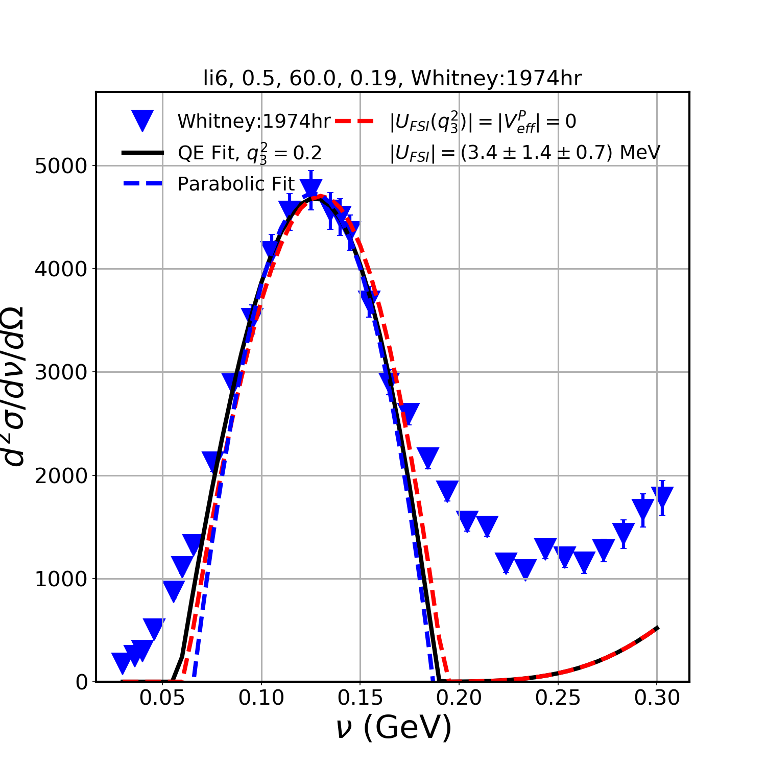
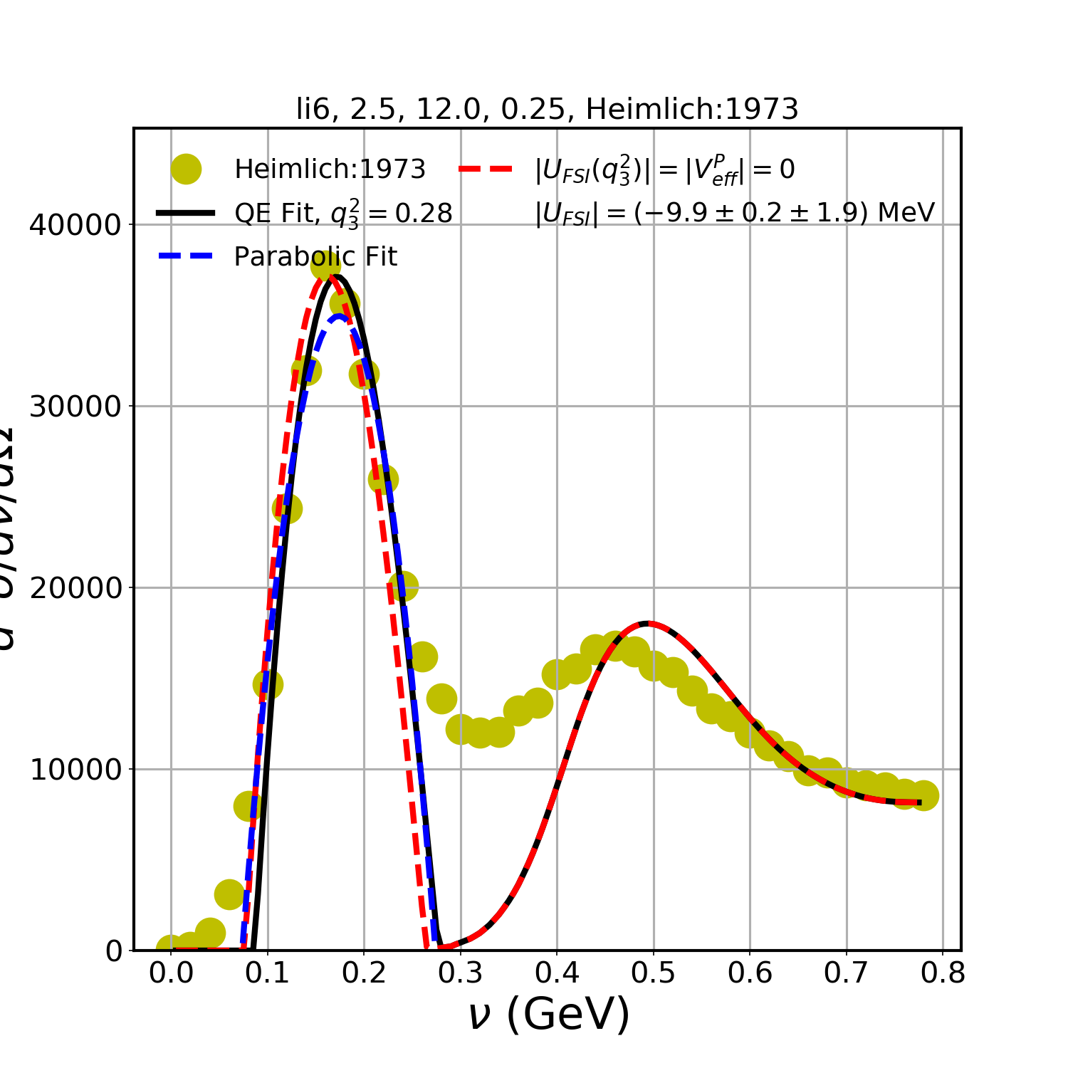
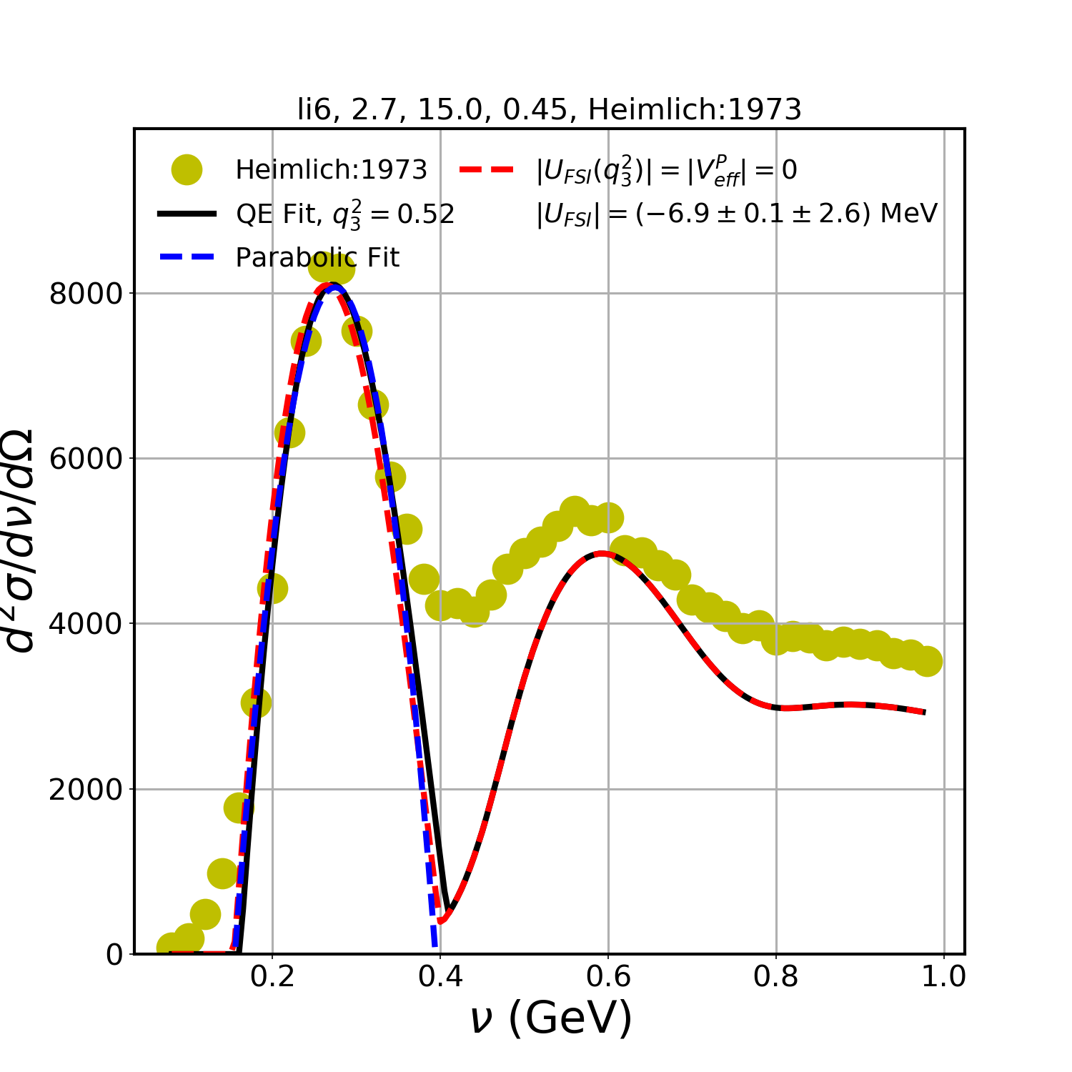
Figure 8: Examples of fits for three out of four ${}_{3}^{6}$Li ($k_{F}^{P}$ = 0.169 GeV) QE differential cross sections. The solid blue curve is the RFG fit with the best value of $U_{FSI}$. The black dashed curve is the simple parabolic fit used to estimate the systematic error. The red dashed curve is the RFG model with $U_{FSI}=V_{eff}=0$. Above each panel we show: The element, $E_{0}$ in GeV, $\theta$ in degrees, $Q^{2}$ in GeV², First Author, and year of publication.

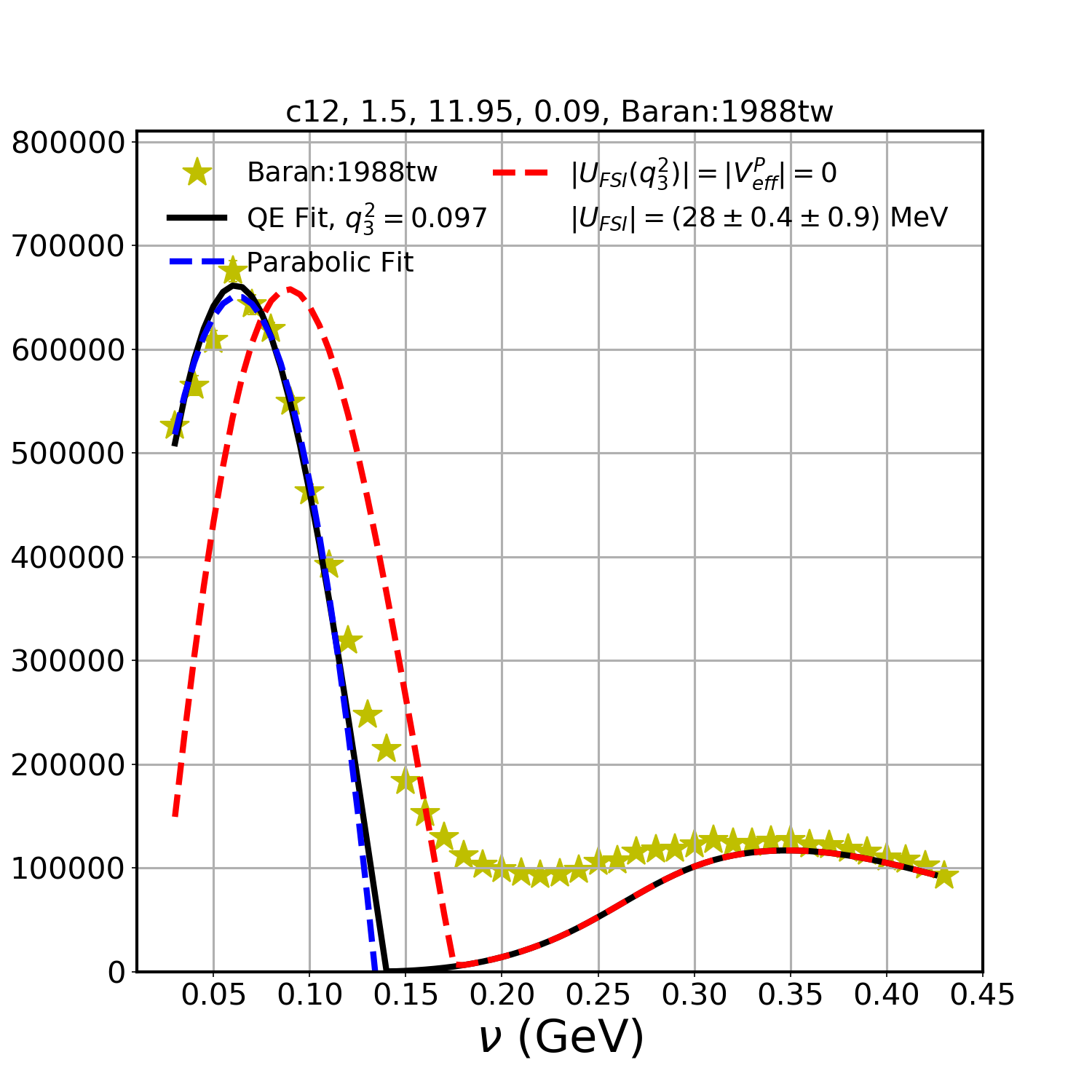
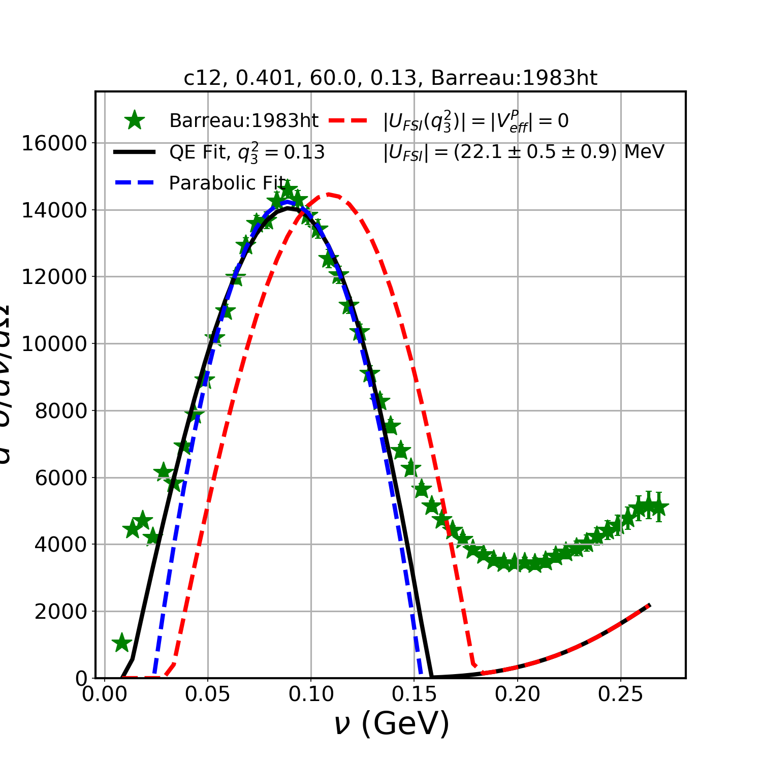
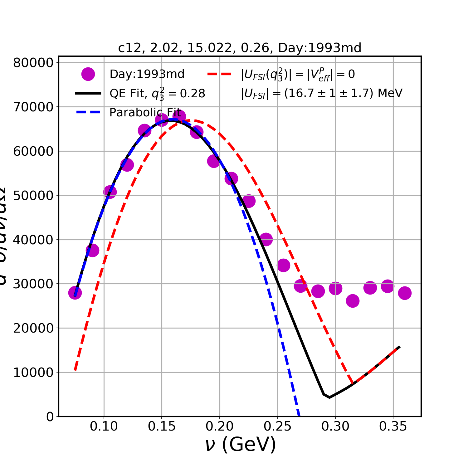
Figure 9: Same as Fig. 8 for three out of 33 ${}_{6}^{12}$C ($k_{F}^{P}$ = 0.221 GeV) QE differential cross sections.

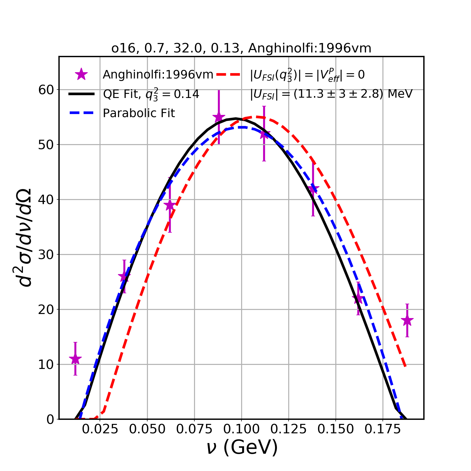
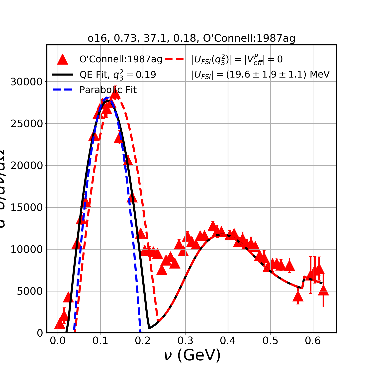
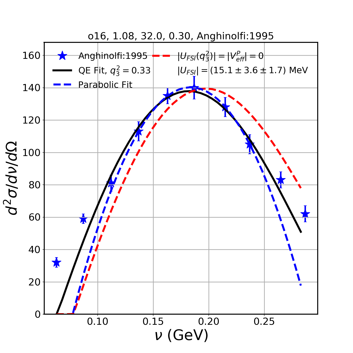
Figure 10: Same as Fig. 8 for three out of 8 ${}_{8}^{16}$O ($k_{F}^{P}$ = 0.225 GeV) QE differential cross sections.

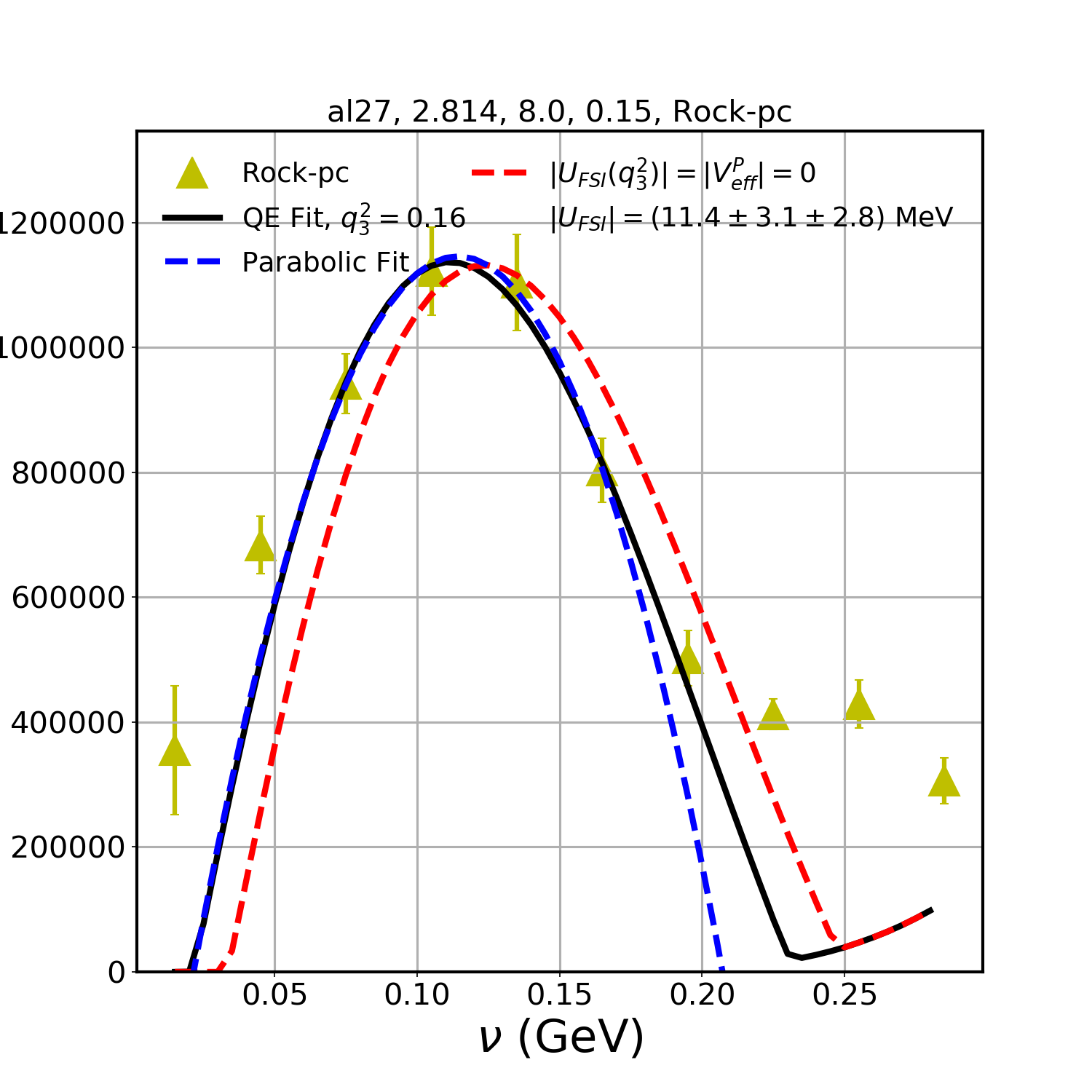
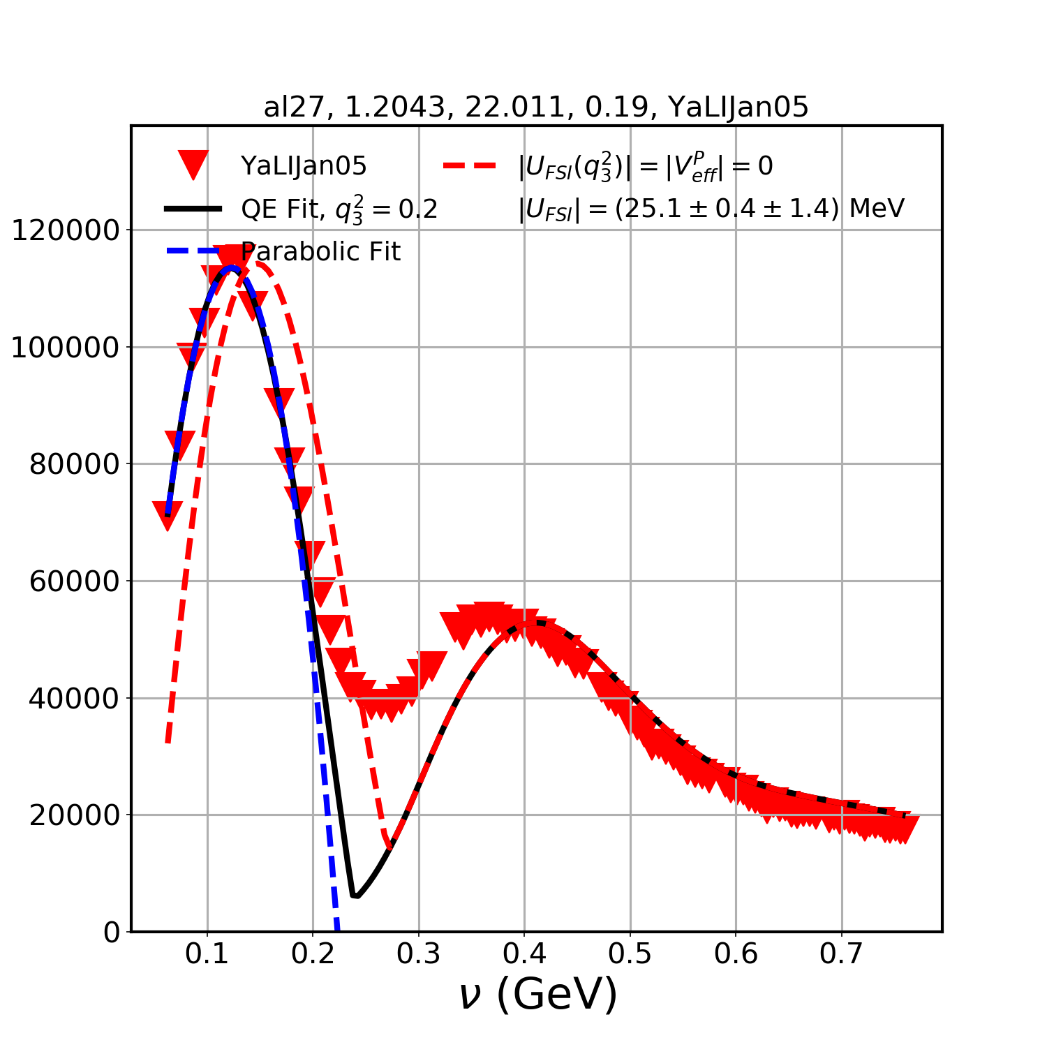
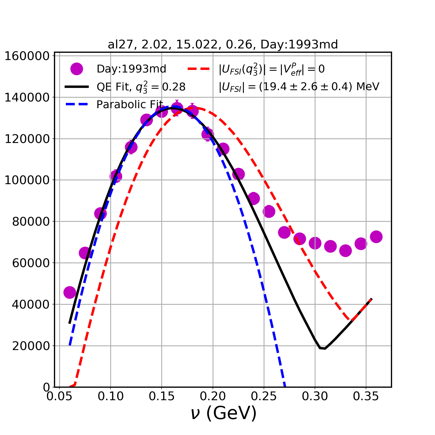
Figure 11: Same as Fig. 8 for three out of 8 ${}_{13}^{27}$Al ($k_{F}^{P}$ = 0.238 GeV) QE differential cross sections.

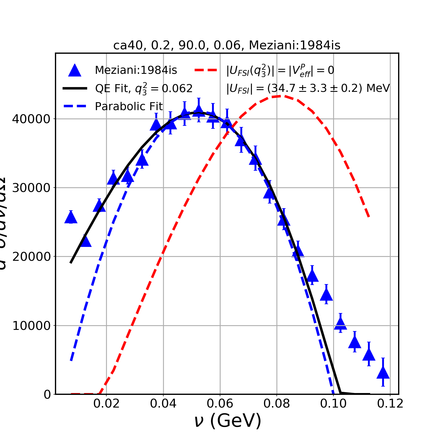
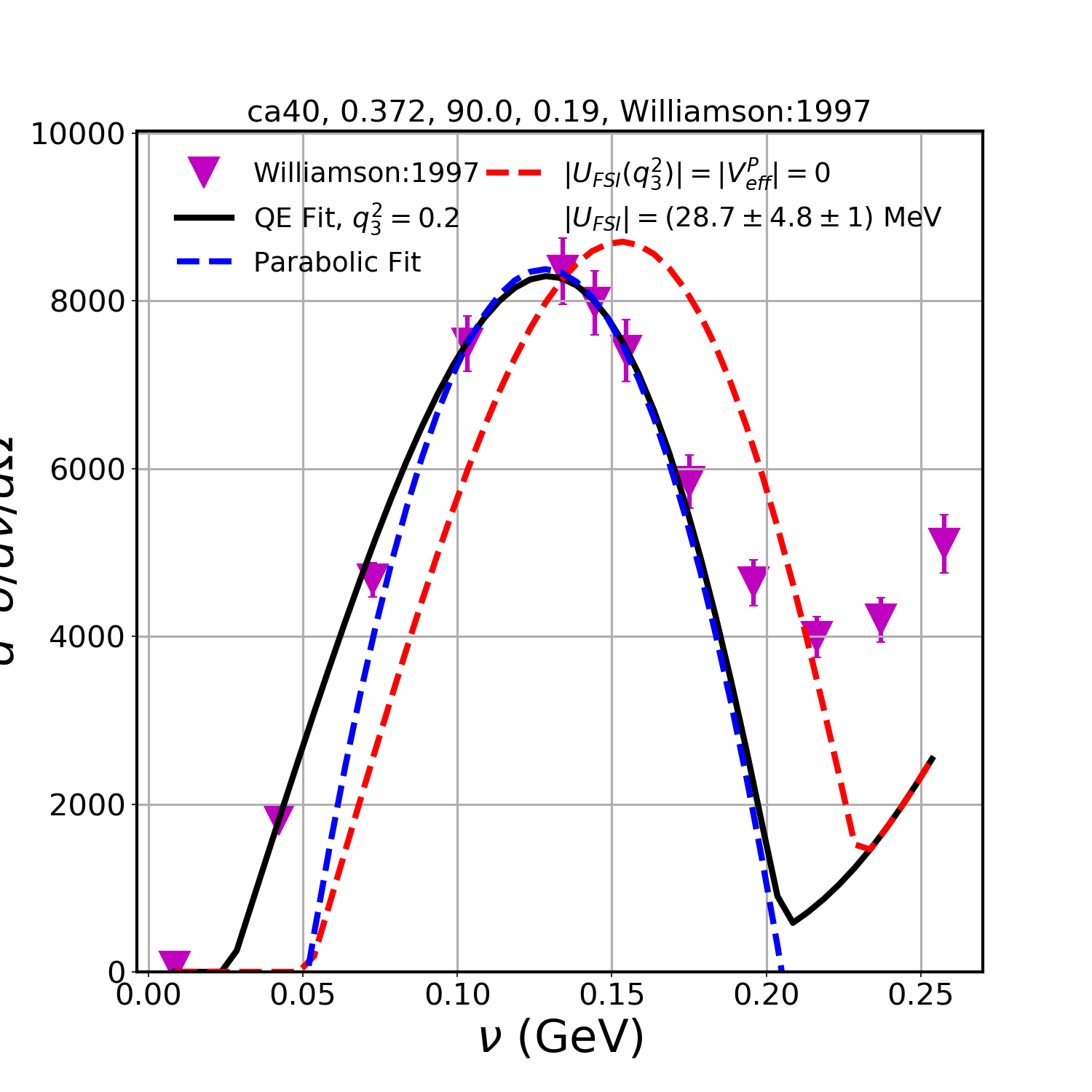
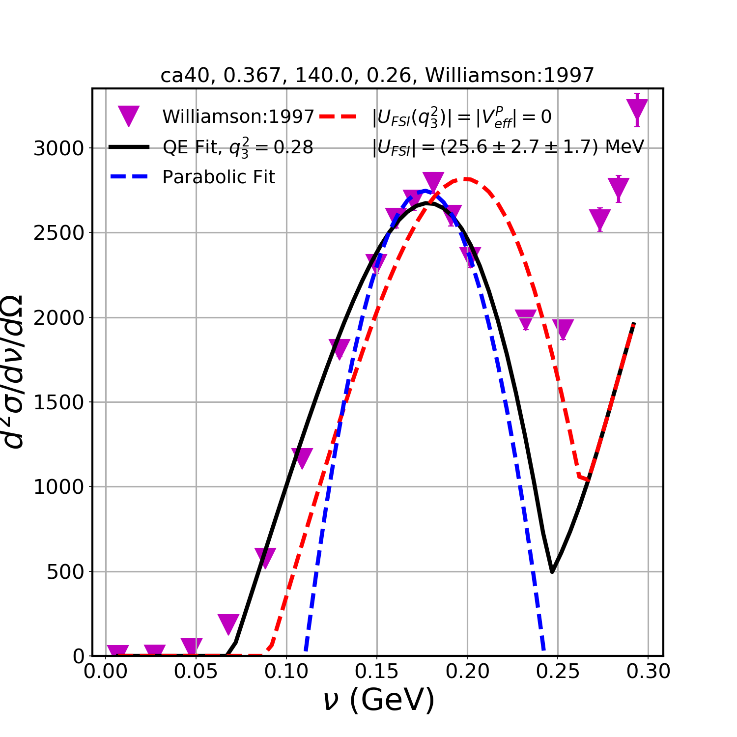
Figure 12: Same as Fig. 8 for three out of 29 ${}_{20}^{40}$Ca ($k_{F}^{P}$ = 0.251 GeV) QE differential cross sections.

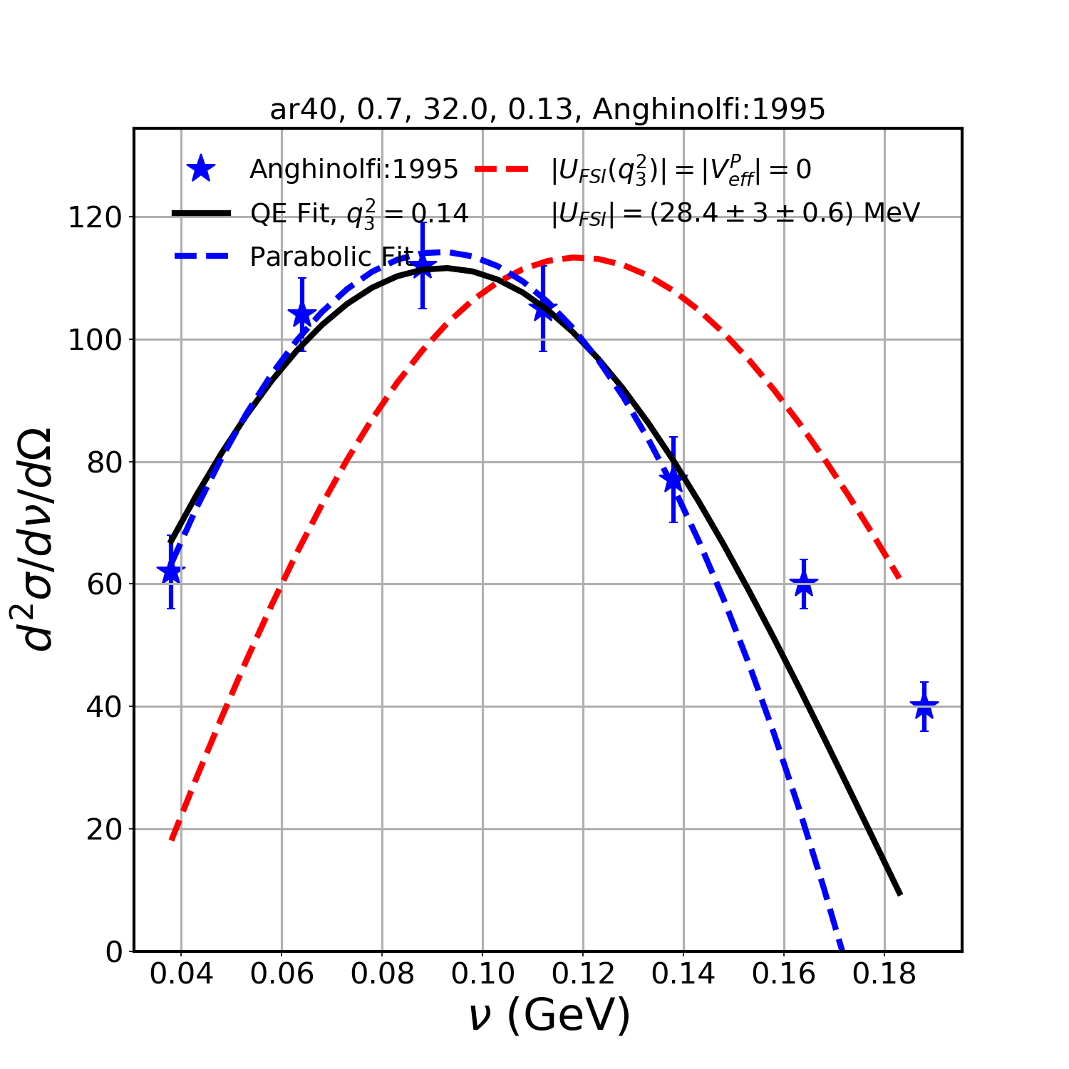
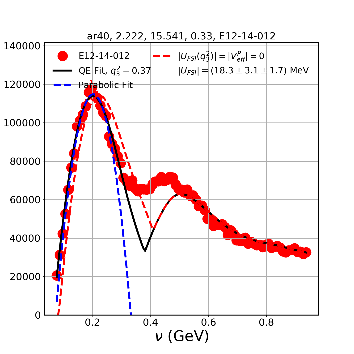
Figure 13: Same as Fig. 8 for two ${}_{18}^{40}$Ar ($k_{F}^{P}$ = 0.251 GeV) QE differential cross sections.

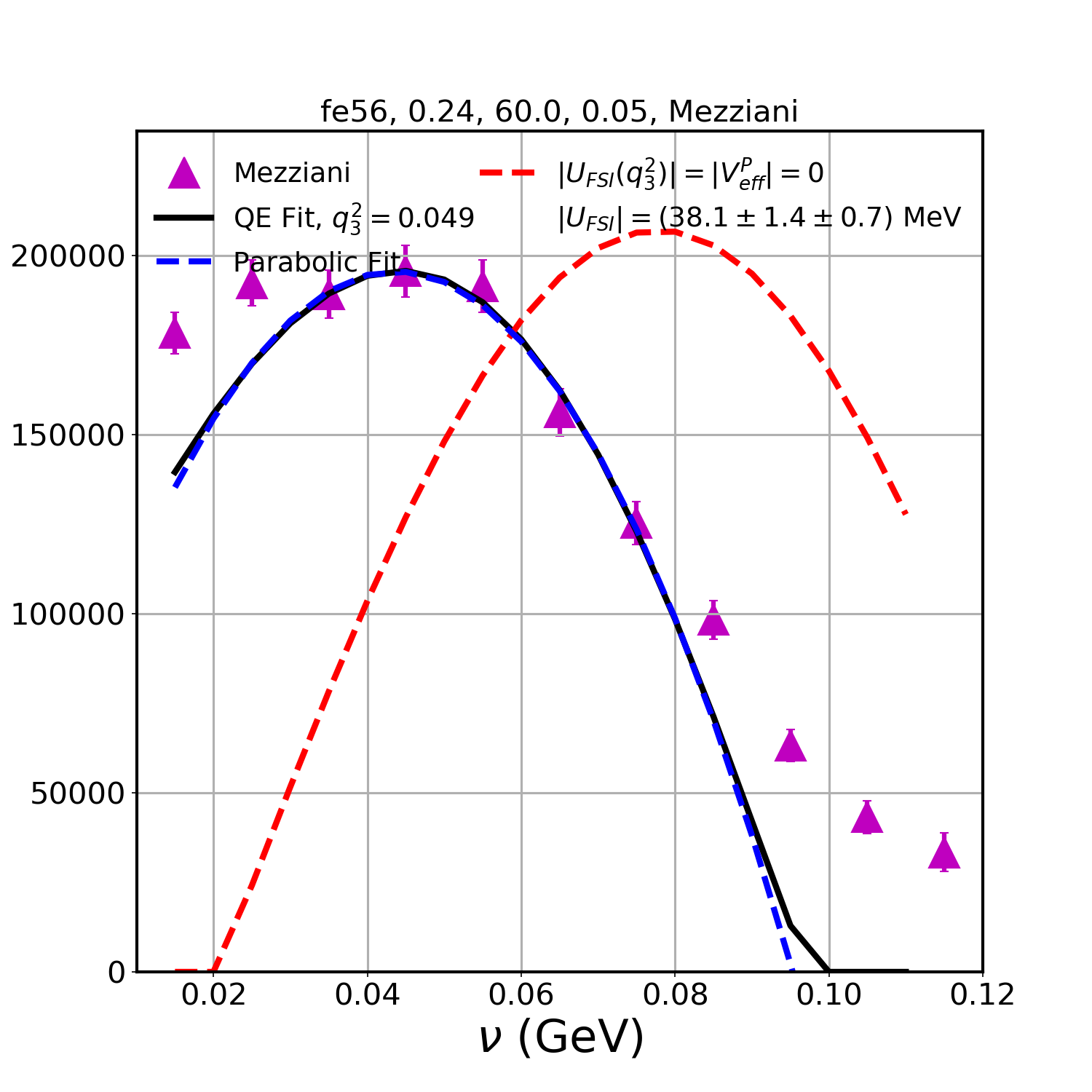
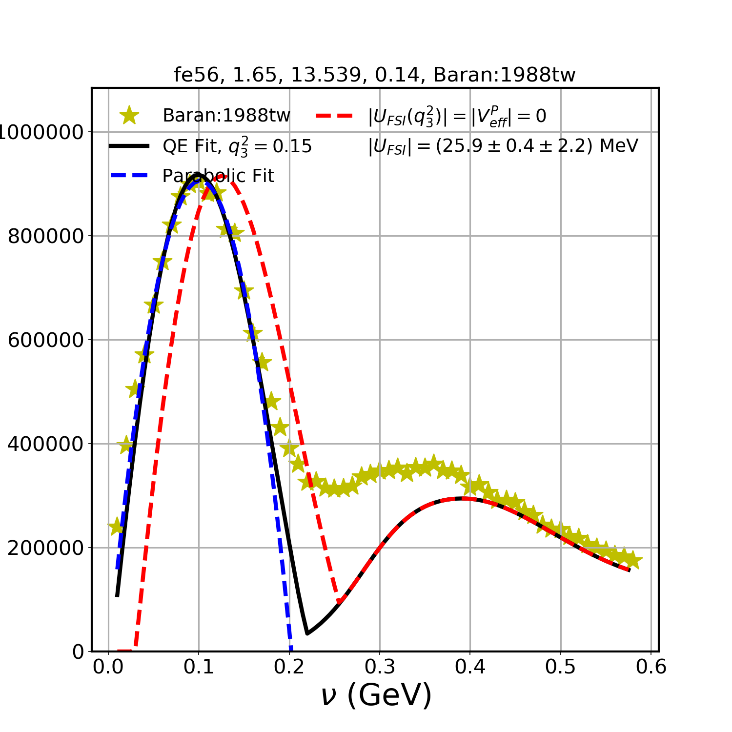
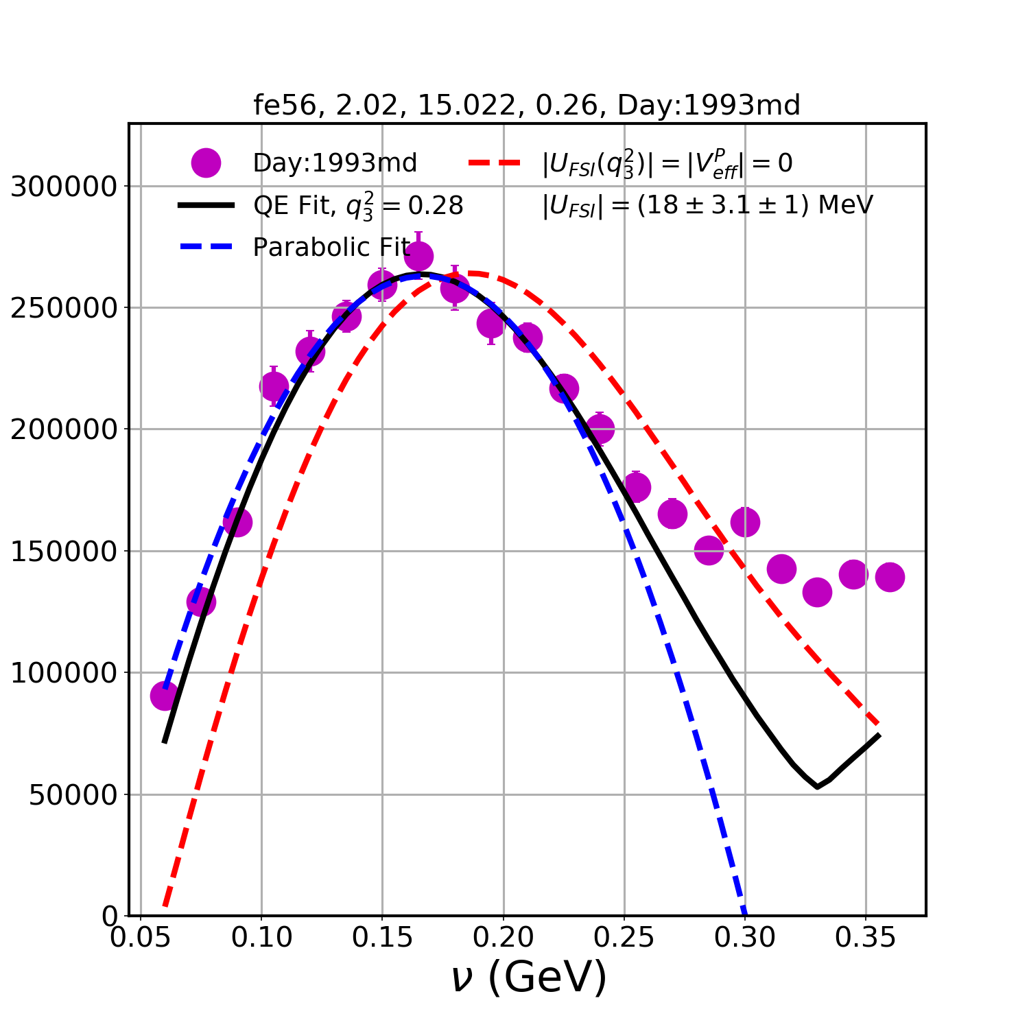
Figure 14: Same as Fig. 8 for three of 30 ${}_{20}^{56}$Fe ($k_{F}^{P}$ = 0.254 GeV) QE differential cross sections.

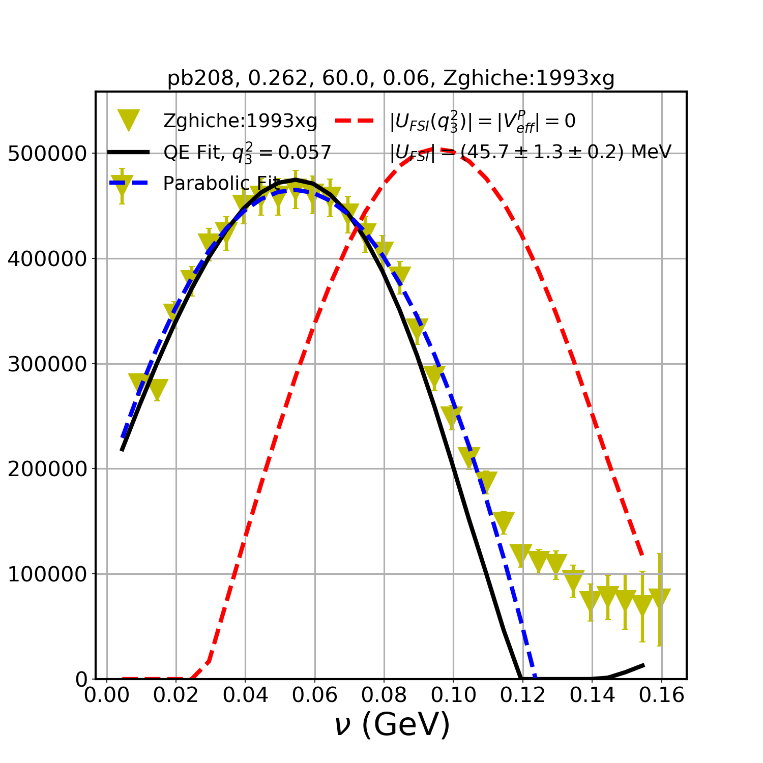
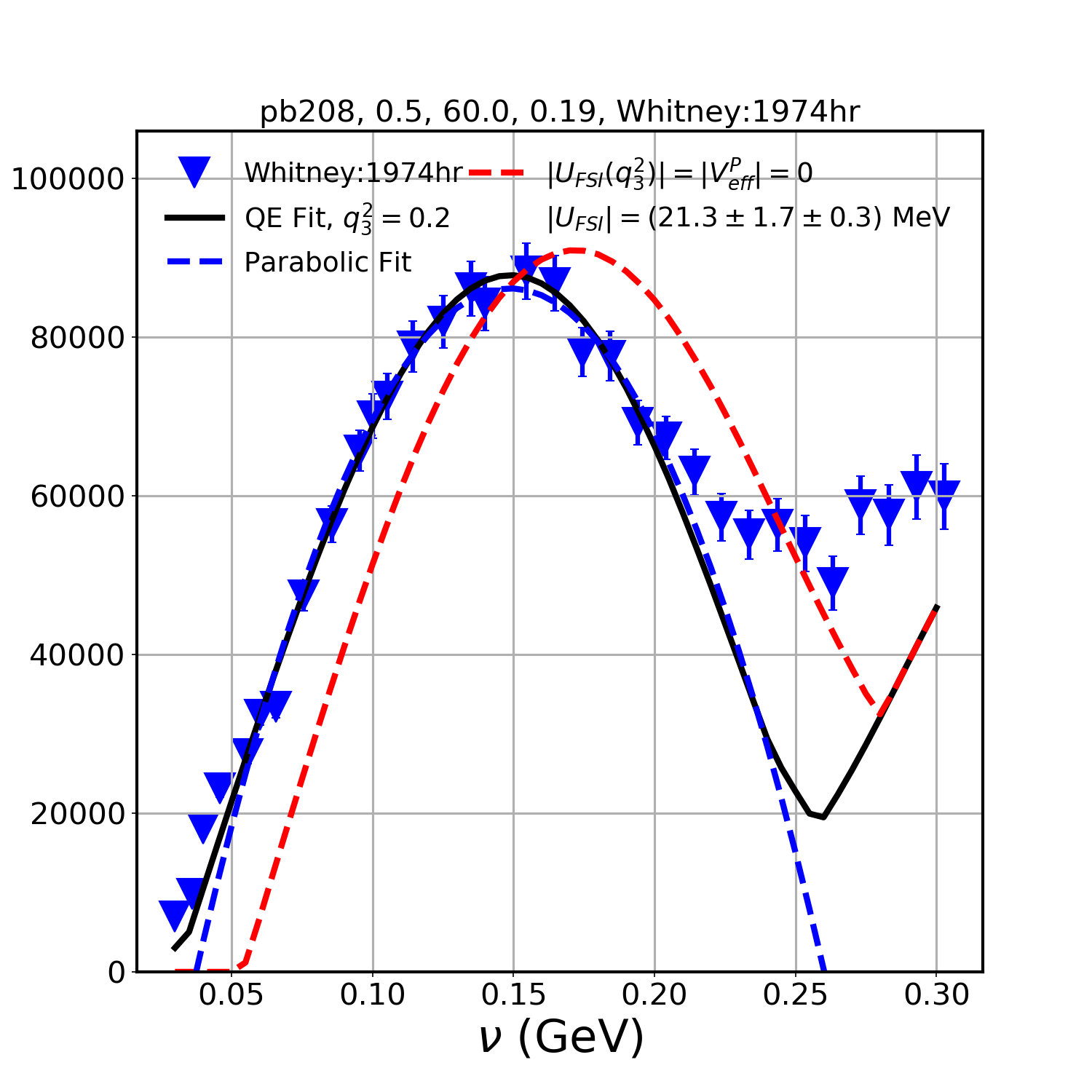
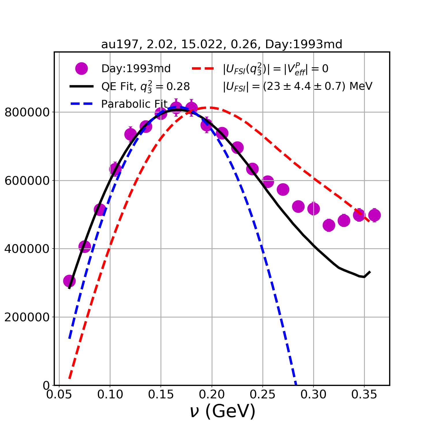
Figure 15: Same as Fig. 8 for two of 22 ${}_{82}^{208}$Pb ($k_{F}^{P}$ = 0.275 GeV) and one ${}_{79}^{197}$Au ($k_{F}^{P}$ = 0.275 GeV) QE differential cross sections.

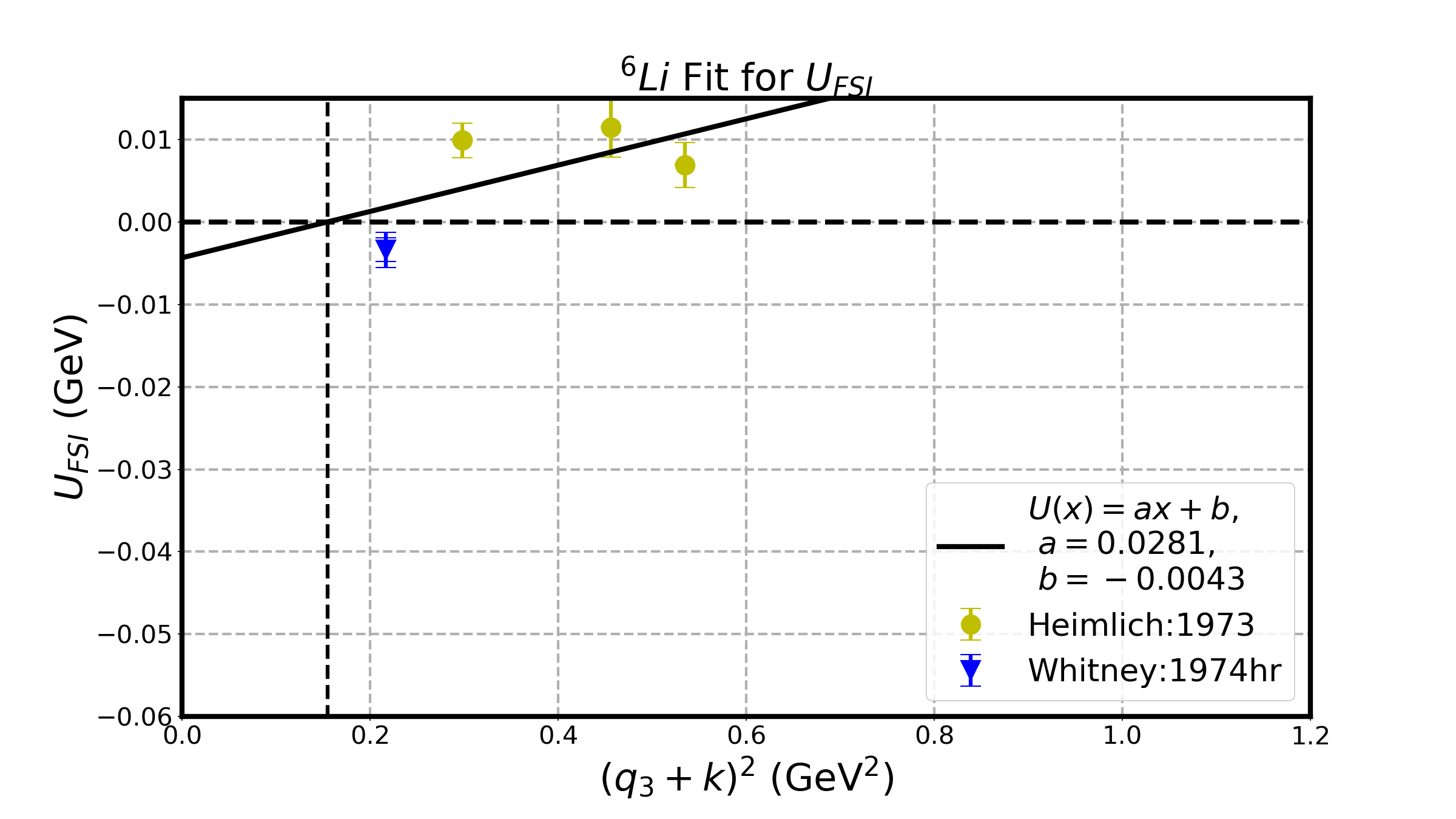
Figure 16: Extracted values of $U_{FSI}$ versus $(\vec{q}_{3}+\vec{k})^{2}$ for four Lithium (${}_{3}^{6}$Li) spectra .

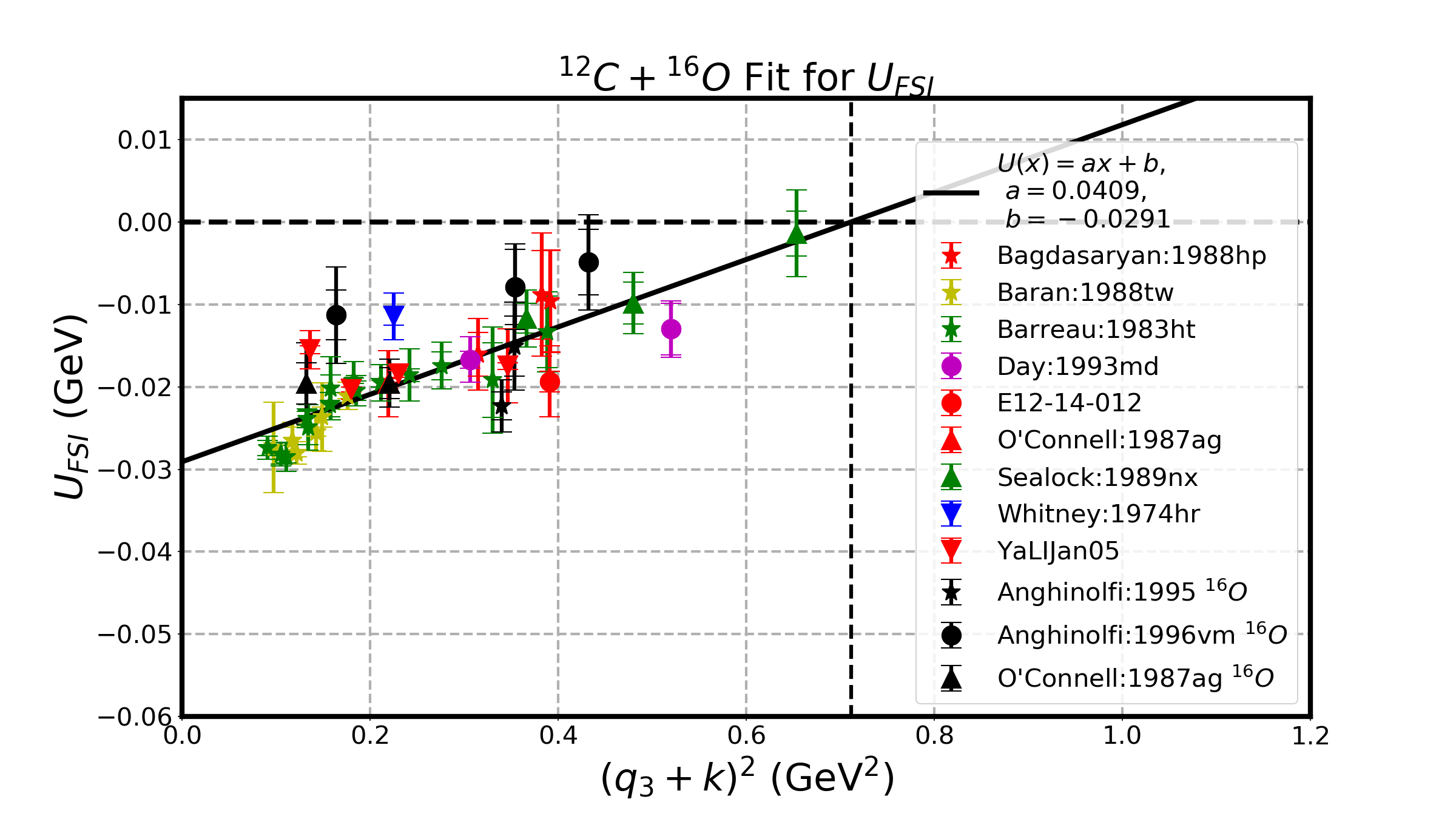
Figure 17: Extracted values of $U_{FSI}$ versus $(\vec{q}_{3}+\vec{k})^{2}$ for 33 Carbon (${}_{6}^{12}$C) and 8 Oxygen (${}_{8}^{16}$O) spectra.

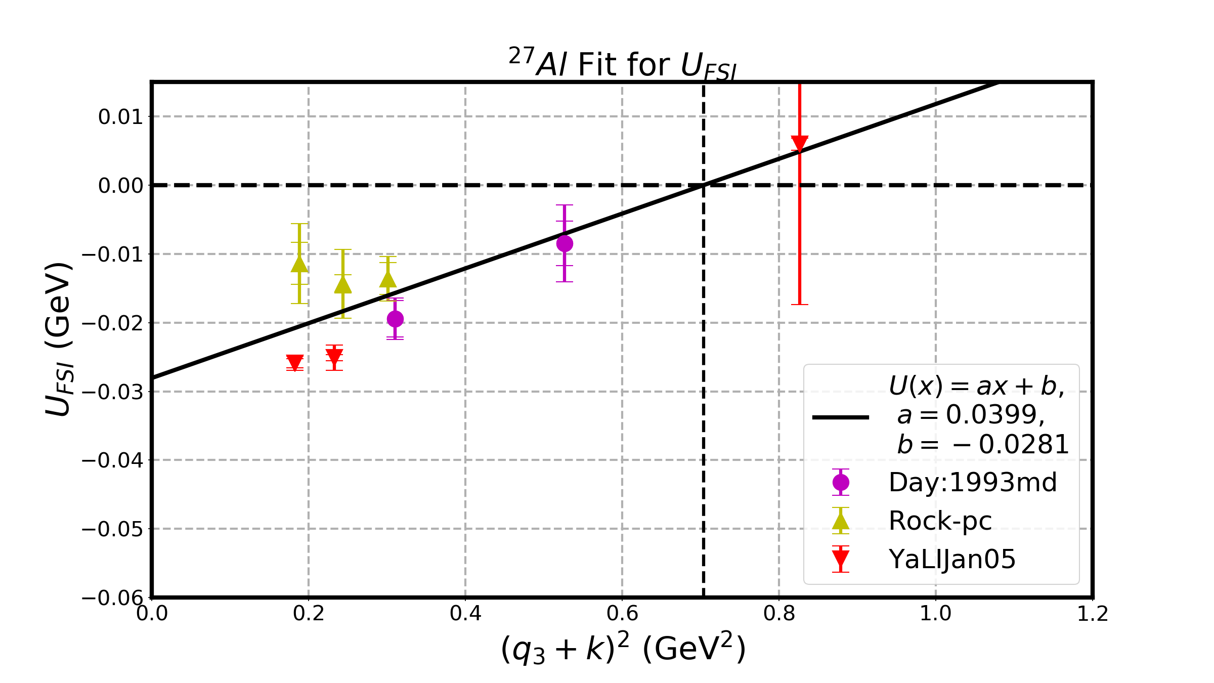
Figure 18: Extracted values of $U_{FSI}$ versus $(\vec{q}_{3}+\vec{k})^{2}$ for 8 Aluminum (${}_{13}^{27}$Al) spectra.

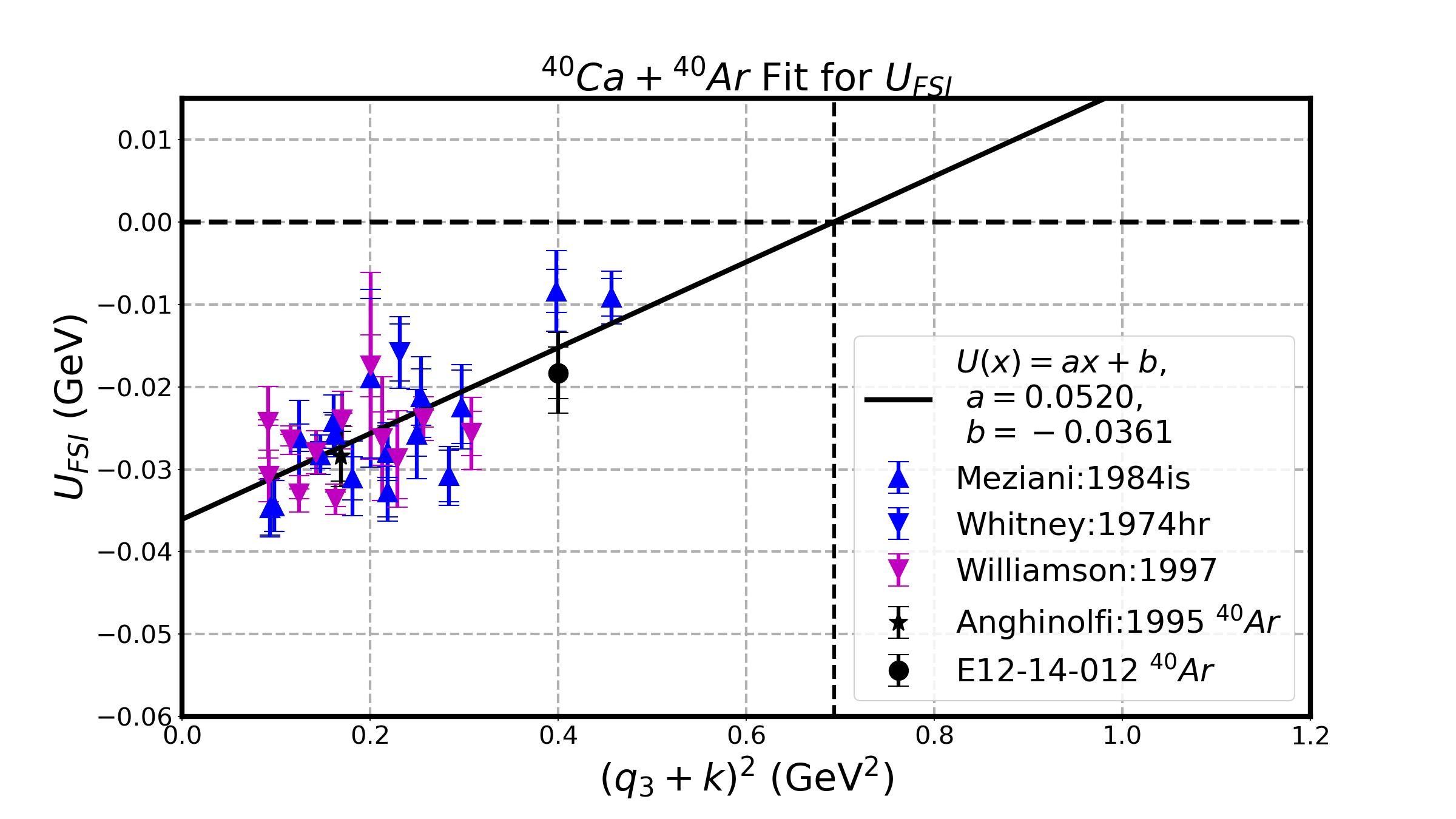
Figure 19: Extracted values of $U_{FSI}$ versus $(\vec{q}_{3}+\vec{k})^{2}$ for 29 Calcium (${}_{20}^{40}$Ca) and 2 Argon ( (${}_{18}^{40}$Ar) spectra

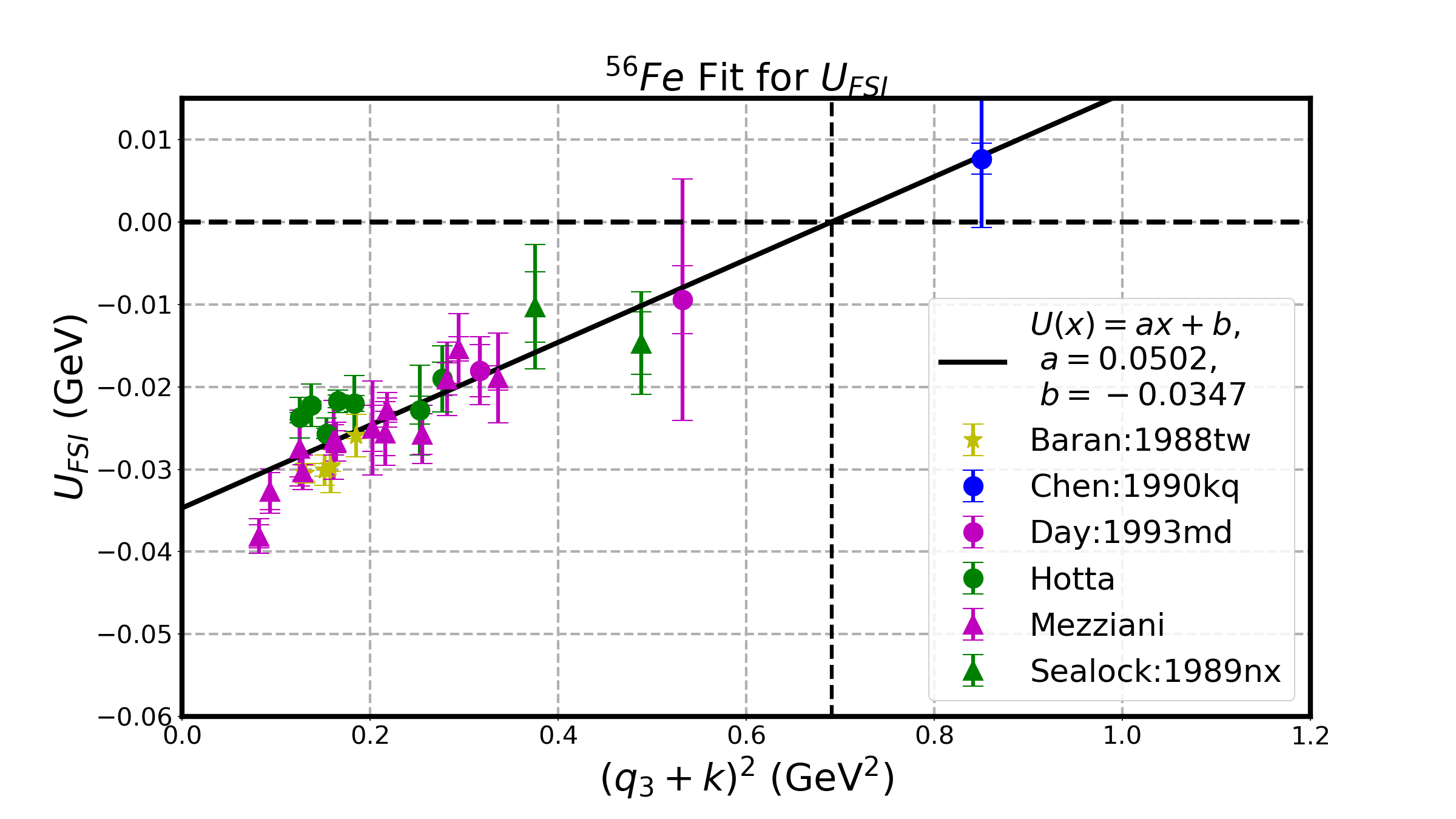
Figure 20: Extracted values of $U_{FSI}$ versus $(\vec{q}_{3}+\vec{k})^{2}$ for 30 Iron (${}_{26}^{56}$Fe) spectra.

Figure 21: Extracted values of $U_{FSI}$ versus $(\vec{q}_{3}+\vec{k})^{2}$ for 22 Lead (${}_{82}^{208}$Pb) and one Gold (${}_{79}^{197}$Au) spectra.

Figure 22: 1p1h process: Neutrino (left) and antineutrino (right) QE scattering from an off-shell bound nucleon of momentum $\vec{p_{i}}$=$\vec{k}$ in a nucleus of mass A. The off-shell energy of the interacting nucleon is $E_{i}^{N,P}=M_{N,P}-\epsilon^{N,P}$, where $\epsilon^{N,P}=S^{N,P}+\langle E_{x}^{N,P}\rangle+\frac{\vec{k}^{2}}{2M^{*}_{A-1}}$. We model the effect of FSI (strong and EM interactions) by setting the energy of the final state proton $E_{f}^{P}=\sqrt{(\vec{k}+\vec{q_{3}})^{2}+M_{P}^{2}}-|U_{FSI}|$+$|V_{eff}^{P}|$ for neutrino QE scattering on bound neutrons, and the energy of the final state neutron $E_{f}^{N}=\sqrt{(\vec{k}+\vec{q_{3}})^{2}+M_{P}^{2}}-|U_{FSI}|$ for antineutrinos scattering on bound protons. Here $U_{FSI}=U_{FSI}((\vec{q}_{3}+\vec{k})^{2})$. For neutrino QE scattering on bound neutrons $|V_{eff}^{P}|=|V_{eff}|$, and the effective ${\mu-}$ energy at the vertex is $E^{\prime}_{\mu-}=E_{\mu-}+V_{eff}$. For antineutrino QE scattering on bound protons $|V_{eff}^{N}|=0$ for the final state neutron and the effective ${\bar{\mu}}$ energy at the vertex is $E^{\prime}_{\bar{\mu}}=E_{\bar{\mu}}-V_{eff}$.

$\bf{}_{Z}^{A}Nucl$	$|V_{eff}|$	$U_{FSI}$	$U_{FSI}$
		intercept	slope vs
	GeV	$(\vec{q}_{3}+\vec{k})^{2}$=0.	$(\vec{q}_{3}+\vec{k})^{2}$
$\bf{}_{3}^{6}Li$	0.0014	-0.0043	0.0281
$\bf{}_{6}^{12}C/\bf_{8}^{16}O$	0.0031	-0.0291	0.0409
$\bf{}_{13}^{27}Al$	0.0051	-0.0281	0.0399
$\bf{}_{20}^{40}Ca/\bf_{18}^{40}Ar$	0.0074/0.0063	-0.0361	0.0520
$\bf{}_{26}^{56}Fe$	0.0089	-0.0347	0.0502
$\bf{}_{82}^{208}Pb/\bf_{79}^{197}Au$	0.0189/0.0185	-0.0360	0.0627

Table 9: The intercepts (GeV) at $\vec{q_{3}^{2}}$=0 and slopes (GeV/GeV²) of fits to $U_{FSI}$ versus $(\vec{q}_{3}+\vec{k})^{2}$. The overall systematic errors on $U_{FSI}$ are estimated at $\pm$0.005 GeV.

7 Implementation for neutrino experiments

For QE scattering of $neutrinos$ ($antineutrinos$) on bound neutrons (protons) the final state nucleon is a proton (neutron). The following equations should be used in neutrino/antineutrino MC generators:

For neutrino QE scattering on bound neutrons:

$$\nu+(M_{N}-\epsilon^{N})=\sqrt{{\bf(k+\vec{q}_{3})^{2}}+M_{P}^{2}}-|U_{FSI}|+|V_{eff}^{P}|$$ (19)

where $|V_{eff}^{P}|=|V_{eff}|$.

For antineutrino QE scattering on bound protons:

$$\nu+(M_{P}-\epsilon^{P})=\sqrt{{\bf(k+\vec{q}_{3})^{2}}+M_{N}^{2}}-|U_{FSI}|$$ (20)

Where

$$\epsilon^{N,P}=S^{N,P}+\langle E_{x}^{N,P}\rangle+\frac{\langle k^{2}\rangle}{2M_{A-1}^{*}}$$ (21)

Rearranging, we have

$$\nu+(M_{N,P}-x^{\nu,\bar{\nu}})=\sqrt{{\vec{(}k+\vec{q}_{3})^{2}}+M_{P,N}^{2}}$$ (22)

where for neutrinos and antineutrinos we have:

$$x^{\nu}((\vec{q}_{3}+\vec{k})^{2}) = \epsilon^{N}-|U_{FSI}|+|V_{eff}^{P}|$$ (23)

$$x^{\bar{\nu}}((\vec{q}_{3}+\vec{k})^{2}) = \epsilon^{P}-|U_{FSI}|$$ (24)

and

$$Q^{2} =-m_{\mu,\bar{\mu}}^{2}+2E_{\nu,\bar{\nu}}(E_{\mu,\bar{\mu}}^{\prime}-\sqrt{(E_{\mu,\bar{\mu}}^{\prime})^{2}-m_{\mu,\bar{\mu}}^{2}}\cos\theta_{\mu,\bar{\mu}})$$ (25)

$$E_{\mu,\bar{\mu}} =E_{\nu,\bar{\nu}}-\nu~{};~{}~{}~{}~{}~{}~{}~{}\vec{q}_{3}^{2}=Q^{2}+\nu^{2}$$

$$E^{\prime}_{\mu} =E_{\mu}+|V_{eff}|~{};~{}~{}~{}~{}~{}~{}~{}E^{\prime}_{\bar{\mu}}=E_{\bar{\mu}}-|V_{eff}|$$

$$E_{f}^{P,N} =\nu-\epsilon^{N,P}$$

For both neutrinos and antineutrinos $\epsilon^{P,N}$ is the unobserved removal energy.

In neutrino experiments in which both the final state lepton and final state proton (or neutron) are measured (e.g. nova, miner$\nu$a, dune) the neutrino energy can be calculated as follows:

$$E_{\nu,\bar{\nu}} = E_{\mu,\bar{\mu}}+E_{f}^{P,N}+\epsilon^{N,P}$$

$$\epsilon^{N,P} = S^{N,P}+\langle E_{x}^{N,P}\rangle+T_{A-1}^{N,P}$$ (26)

$$T_{A-1}^{N,P} = \frac{\langle(k^{N,P})^{2}\rangle}{2M_{A-1}}=\frac{3}{5}\frac{(k_{F}^{N,P})^{2}}{2M_{A-1}}$$

8 Corrections to GENIE version 2

The generation of events in $\textsc{genie}~{}2$ as currently done is equivalent to using equations 19 and 20, but with $V_{eff}=0$, $U_{FSI}=0$, and $\langle E_{x}^{P,N}\rangle$=0. In addition, an amount $\Delta^{\text{nucleon}}_{\textsc{genie}}$ (25 MeV for ${}^{12}_{6}C$) is subtracted from the energy of the final state nucleon (or quark for inelastic events) to account for “binding energy” in $\textsc{genie}~{}2$. For neutrino QE scattering on bound neutrons events are generated in $\textsc{genie}~{}2$ using the following equations:

$$\nu_{\textsc{genie}}^{\nu,\bar{\nu}}+(M_{N,P}-x_{\textsc{genie}}^{\nu,\bar{\nu}}) = \sqrt{{\bf(k+\vec{q}_{3})^{2}}+M_{P,N}^{2}}$$

$$\epsilon_{\textsc{genie}}^{\nu,\bar{\nu}}=x_{\textsc{genie}}^{\nu,\bar{\nu}};~{}~{}~{}~{}~{}~{}~{}x_{\textsc{genie}}^{\nu,\bar{\nu}} = S^{N,P}+\frac{\langle k^{2}\rangle}{2M_{A-1}}$$ (27)

Where $\epsilon_{\textsc{genie}}^{\nu,\bar{\nu}}$ is the removal energy for neutrino (antineutrino) assumed in genie . Therefore the difference between the correct muon energy and the muon energy generated by genie is approximately equal to $\Delta x^{\nu}_{\textsc{genie}}=x^{\nu}-x_{\textsc{genie}}$.

$$\Delta x^{\nu}_{\textsc{genie}} = \langle E_{x}^{N}\rangle-|U_{FSI}|+|V_{eff}^{P}|$$ (28)

$$\Delta x^{\bar{\nu}}_{\textsc{genie}} = \langle E_{x}^{P}\rangle-|U_{FSI}|$$

$$\Delta\epsilon_{\textsc{genie}}^{\nu,\bar{\nu}} = \langle E_{x}^{N,P}\rangle$$

$$\Delta\nu_{\textsc{genie}}^{\nu,\bar{\nu}} = \nu^{\nu,\bar{\nu}}-\nu_{\textsc{genie}}^{\nu,\bar{\nu}}$$

$$\approx \Delta x^{\nu,\bar{\nu}}_{\textsc{genie}}$$

$$\Delta(E_{\mu})_{\textsc{genie}} = E_{\mu}-(E_{\mu})_{\textsc{genie}}$$

$$= -\Delta\nu_{\textsc{genie}}^{\nu,\bar{\nu}}$$

$$\Delta(E_{f}^{P,N})_{\textsc{genie}} = E_{f}^{P,N}-(E_{f}^{P,N})_{\textsc{genie}}$$

$$= \Delta\nu_{\textsc{genie}}^{\nu,\bar{\nu}}-\langle E_{x}^{N,P}\rangle+\Delta^{\text{nucleon}}_{\textsc{genie}}$$

Where $\Delta^{\text{nucleon}}_{\textsc{genie}}$= 25 MeV is used in genie.

As given in the Tables 7 and 8, $\langle E_{x}^{P,N}\rangle$ for Carbon is equal to 10.1 MeV and 10.0 MeV for protons and neutrons, respectively and $|V_{eff}|$=3.1 MeV.

For Oxygen $\langle E_{x}^{P,N}\rangle$ is equal to 10.9 MeV and 10.2 MeV for protons and neutrons, respectively, and $|V_{eff}|$=3.4 MeV.

For Argon $\langle E_{x}^{P,N}\rangle$ is equal to 17.8 MeV and 21.8 MeV for protons and neutrons, respectively, and $|V_{eff}|$=6.3 MeV.

Tables 10 and 11 show the differences between the correctly simulated muon, final state nucleon and removal (unobserved) energies and those generated by genie 2 for QE events in carbon, and oxygen respectively. These differences are shown for the case of $\vec{q}_{3}^{2}$ = 0.2 GeV² ($|U_{FSI}|$ = 20 MeV) and for $\vec{q}_{3}^{2}$= 0.8 GeV² ($|U_{FSI}|$ = 0).

Carbon	$\vec{q}_{3}^{2}$	$\Delta E_{\mu+,\mu-}$	$\Delta E_{f}^{P,N}$	$\Delta\epsilon^{P,N}$
MC	GeV2	$MeV$	$MeV$	MeV
$U_{FSI}$= 20.0 MeV	0.2
$\textsc{genie}~{}\nu$		+6.9	+8.1	+10.0
$\textsc{genie}~{}\bar{\nu}$		+9.9	+5.0	+10.1
$U_{FSI}$= 0.0 MeV	0.8
$\textsc{genie}~{}\nu$		-13.1	+28.1	+10.0
$\textsc{genie}~{}\bar{\nu}$		-10.1	+25.0	+10.1

Table 10: Estimates of the difference between the correctly simulated muon, final state nucleon and removal (unobserved) energies and those generated by $\textsc{genie}~{}2$ for QE events in carbon.

Oxygen	$\vec{q}_{3}^{2}$	$\Delta E_{\mu+,\mu-}$	$\Delta E_{f}^{P,N}$	$\Delta\epsilon^{P,N}$
MC	GeV2	$MeV$	$MeV$	MeV
$U_{FSI}$= 20.0 MeV	0.2
$\textsc{genie}~{}\nu$		+6.4	+8.4	+10.2
$\textsc{genie}~{}\bar{\nu}$		+9.1	+5.0	+10.9
$U_{FSI}$= 0.0 MeV	0.8
$\textsc{genie}~{}\nu$		-13.6	+28.4	+10.2
$\textsc{genie}~{}\bar{\nu}$		-10.9	+25.0	+10.9

Table 11: Difference between the correctly simulated muon, nucleon and removal (unobserved) energies and those generated by $\textsc{genie}~{}2$ for QE events in Oxygen.

9 Conclusion

We investigate the binding energy parameters that should be used in modeling electron and neutrino scattering from nucleons bound in a nucleus within the framework of the impulse approximation. We discuss the relation between binding energy, missing energy, removal energy ($\epsilon$), spectral functions and shell model energy levels and extract updated removal energy parameters from ee^′p spectral function data. We address the difference in parameters for scattering from bound protons and neutrons. We also use inclusive e-A data to extract an empirical parameter $U_{FSI}((\vec{q}_{3}+\vec{k})^{2})$ to account for the interaction of final state nucleons (FSI) with the optical potential of the nucleus. Similarly we use $V_{eff}$ to account for the Coulomb potential of the nucleus.

With three parameters $\epsilon$, $U_{FSI}((\vec{q}_{3}+\vec{k})^{2})$and $V_{eff}$ we can describe the energy of final state electrons for all available electron QE scattering data. The use of the updated parameters in neutrino Monte Carlo generators reduces the systematic uncertainty in the combined removal energy (with FSI corrections) from $\pm$ 20 MeV to $\pm$ 5 MeV.

Appendix A Appendix: Coulomb corrections

For targets with atomic number Z greater than one we should take into account the effect of the electric field of the nucleus on the incident and scattered electrons (and also on the final state proton in QE events). These corrections are called Coulomb corrections. For atomic weight A and atomic number Z the protons create an electrostatic potential V(r). In the effective momentum approximation (EMA), the effective potential for an incident electron is $V_{eff}$, which can be calculated as follows:

$$V(r) = \frac{3\alpha(Z)}{2R}+\frac{r\alpha(Z)}{2R^{2}}$$

$$R = 1.1A^{1/3}+0.775A^{-1/3}$$

$$V_{eff} = -0.8V(r=0)=-0.8\frac{3\alpha(Z)}{2R}.$$ (29)

The values for $|V_{eff}|$ calculated from equation 29 agree (within errors) with values extracted from a comparison of the peak positions and cross sections of positron and electron QE scatteringgueye . For our estimates of $|V_{eff}|$ shown in Table 7 we use the experimental values for the nuclei that were measured in ref.gueye . We use equation 29 to interpolate to other nuclei.

For electrons scattering on bound nucleons the effective incident energy is $E_{eff}=E_{0}+|V_{eff}|$, and the effective scattered energy is $E^{\prime}_{eff}=E^{\prime}+|V_{eff}|$. This implies that the effective square of the momentum transfer is increased. For positrons scattering on bound nucleons the effective incident energy is $E_{eff}=E_{0}-|V_{eff}|$, and the effective scattered energy is $E^{\prime}_{eff}=E^{\prime}-|V_{eff}|$. This implies that the effective square of the momentum transfer is decreased.

For electron QE scattering on bound protons $|V_{eff}^{P}|=\frac{Z-1}{Z}|V_{eff}|$. For neutrino QE scattering on bound neutrons $|V_{eff}^{P}|=|V_{eff}|$. For neutrino QE scattering on bound protons $|V_{eff}^{N}|=0$.

For completeness, though not relevant in this analysis, there is also a focusing factor $F_{foc}=(\frac{E_{0}+|V_{eff}|}{E_{0}})^{2}$ that enhances the cross section for electrons and reduces the cross section for positrons. The focussing factor cancels the $1/E_{0}^{2}$ factor in the Mott cross section. Therefore, the Coulomb correction should only be applied to the structure functions $W_{1}$ and $W_{2}$.

Appendix B Appendix: Relativistic Fermi Gas (RFG)

For the Fermi gas model the momentum distribution is zero for $k>k_{F}$, and for $k<k_{F}$ it is given by

$$|\phi(k)|^{2} = \frac{1}{N_{rfg}}~{}~{}~{}~{}~{}~{}~{}~{}N_{rfg}=\frac{4}{3}{\pi}K_{F}^{3}$$

$$P_{rfg}(k)dk = |\phi(k)|^{2}4\pi\vec{k}^{2}dk=\frac{1}{N_{rfg}}{4\pi\vec{k}^{2}dk,}$$ (30)

and $\langle\vec{k}^{2}\rangle=(3/5)k_{F}^{2}$.

B.1 Distributions and parameters of RFG versus $k_{z}$

Here we do the calculation in cylindrical coordinates

$$(2\pi\vec{k}^{2}~{}d\cos\theta~{}dk=\pi dk_{T}^{2}~{}dk_{z})$$

$$k=\sqrt{k_{T}^{2}+k_{z}^{2}}.$$

the probability distribution of the Z component of the momentum $k_{z}$ $P(k_{z})~{}dk_{z}$, and average square of the transverse momentum $\langle k_{T}^{2}(k_{Z})\rangle$ as a function of $k_{z}$ are given below.

$$P(k_{z})_{rfg}dk_{z} = \frac{3(1-k_{z}^{2}/k_{F}^{2})}{4k_{F}}dk_{z}$$ (31)

$$\langle k_{T}^{2}(k_{z})_{rfg}\rangle = \frac{1}{2}{k_{F}^{2}}(1-k_{z}^{2}/k_{F}^{2})$$ (32)

$$\langle\vec{k}^{2}(k_{z})_{rfg}\rangle = \langle k_{T}^{2}(k_{z})_{rfg}\rangle+k_{z}^{2}$$ (33)

B.2 Pauli Blocking

We multiply the QE differetial cross sections by a Pauli blocking factor $K_{Pauli}^{nuclei}(\vec{q}_{3}^{2})$ which reduces the predicted cross sections at low $\vec{q}_{3}^{2}$. The Pauli suppression factor shown below is from Eq. B54 of reference Tsai .

$$K_{Pauli}^{nuclei}=\frac{3}{4}\frac{|\vec{q}_{3}|}{k_{F}}(1-\frac{1}{12}(\frac{|\vec{q}_{3}|}{k_{F}})^{2})$$ (34)

For $|\vec{q}_{3}|<2k_{F}$, otherwise no Pauli suppression correction is made. Here $|\vec{q}_{3}|=\sqrt{Q^{2}+\nu^{2}}$ is the absolute magnitude of the 3-momentum transfer to the target nucleus,

Appendix C Reconstruction of $E_{\nu}^{QE{\text{-}}\mu}$, $Q^{2}_{QE{\text{-}}\mu}$ and $Q^{2}_{QE{\text{-}}P}$

In this section we update the expressions for the mean reconstructed neutrino energy $E_{\nu}^{QE{\text{-}}\mu}$ and square of the four-momentum transfer $Q^{2}_{QE{\text{-}}\mu}$ extracted only from the kinematics of final state muons in QE events. In addition we can also reconstruct the four momentum transfer $Q^{2}_{Q{\text{-}}(P,N)}$ from the kinematics of the final state recoil proton or neutron in QE events.

The expressions are updated to include:

1. The contribution of final state interaction $|U_{FSI}|$.

2. The contribution of Coulomb corrections $V_{eff}$.

3. The contribution of the proton and neutron transverse momentum $\vec{k}_{T}$ at the location of the QE peak.

In the derivation of the expressions we use relativistic kinematics. The ”primed” energies and momenta are at the vertex before FSI with the nuclear and Coulomb field.

$$E_{i}^{N,P} = M_{N,P}-\epsilon^{N,P}$$ (35)

$$E_{f}^{P} = \sqrt{(\vec{k}+\vec{q}_{3})^{2}+M_{P}^{2})}-|U_{FSI}|+|V_{eff}^{P}|$$

$$= E_{F}^{P\prime}-|U_{FSI}|+|V_{eff}^{P}|$$

$$E_{f}^{N} = \sqrt{(\vec{k}+\vec{q}_{3})^{2}+M_{N}^{2})}-|U_{FSI}|$$

$$= E_{F}^{N\prime}-|U_{FSI}|$$

$$E_{\mu{\text{-}}} = E_{\mu{\text{-}}}^{\prime}-|V_{eff}^{P}|,~{}~{}~{}~{}~{}E_{\mu{\text{+}}}=E_{\mu{\text{+}}}^{\prime}+|V_{eff}|$$ (38)

For neutrino scattering on bound neutrons $|V_{eff}^{P}|=|V_{eff}|$. We define $M_{N}$, $M_{P}$, $m_{\mu}$ as the neutron, proton and muon masses. At the peak location of the QE distribution the bound neutron momentum is perpendicular to $\vec{q}$ (i.e. $k_{z}$=0). In this case, the average of the square of transverse momenta of the neutron (proton) for a Fermi gas momentum distribution (and also for a Gaussian distribution) is $\langle\vec{k}_{T{\text{-}}N}^{2}\rangle=\frac{(k_{F}^{N})^{2}}{2}$ for a bound neutron in the initial state and $\langle\vec{k}_{T{\text{-}}P}^{2}\rangle=\frac{(k_{F}^{P})^{2}}{2}$) for bound proton in the initial state.

C.1 Using only the kinematics of the $\mu^{-}$

For $neutrino$ QE events we define $E_{\mu{\text{-}}}^{\prime}=T_{\mu{\text{-}}}+m_{\mu}+|V_{eff}|$ as the total Coulomb corrected muon energy. We define $(M_{P}^{\prime})^{2}=M_{P}^{2}+\langle\vec{k}_{T{\text{-}}N}^{2}\rangle$ to account for the fact that the final state $proton$ has the same average transverse momentum as that of the initial state $neutron$ $\langle\vec{k}_{T{\text{-}}N}^{2}\rangle$ with respect to the neutrino-muon scattering plane. From energy-momentum conservation we get:

$$E_{\nu} = p^{\prime}_{\mu{\text{-}}}\cos\theta_{\mu{\text{-}}}+P^{\prime}_{P}\cos\theta_{P}$$ (39)

$$p^{\prime}_{\mu{\text{-}}}\sin\theta_{\mu} = P^{\prime}_{P}\sin\theta_{P}$$

$$E_{\nu}+M_{N}-\epsilon^{N} = [\sqrt{(P_{P}^{\prime})^{2}+(M_{P}^{\prime})^{2}}]-|U_{FSI}|+|V_{eff}^{P}|$$

$$+ E^{\prime}_{\mu{\text{-}}}-|V_{eff}|$$

$$E_{\nu}+M_{N}^{\prime\prime} = \sqrt{(P_{P}^{\prime})^{2}+(M_{P}^{\prime})^{2}}+E^{\prime}_{\mu{\text{-}}}$$

$$M_{N}^{\prime\prime} = M_{N}-(\epsilon^{N}-|U_{FSI}|).$$

Here. for neutrino scattering on bound neutrons $|V_{eff}^{P}|=|V_{eff}|$, $|U_{FSI}=|U_{FSI}(\vec{q}_{3}^{2}+\frac{1}{2}k_{F}^{2})|$, $p^{\prime}_{\mu{\text{-}}}=\sqrt{(E^{\prime}_{\mu{\text{-}}})^{2}-m_{\mu}^{2}}$, $E_{\mu{\text{-}}}=E_{\mu{\text{-}}}^{\prime}-|V_{eff}|$, $P_{P}^{\prime}$ is the momentum of the final state $proton$ (before FSI) in the $neutrino-muon$ plane, and $\theta_{P}$ is the angle of the proton in the $neutrino-muon$ scattering plane. From equations 39 we obtain the following expressions.

$$E_{\nu}^{QE{\text{-}}\mu} = \frac{2(M_{N}^{\prime\prime})E_{\mu{\text{-}}}-((M_{N}^{\prime\prime})^{2}+m_{\mu}^{2}-(M_{P}^{\prime})^{2})}{2\cdot[(M_{N}^{\prime\prime})-E_{\mu{\text{-}}}+\sqrt{(E_{\mu{\text{-}}})^{2}-m_{\mu}^{2}})\cos\theta_{\mu{\text{-}}}]}$$

$$Q^{2}_{QE{\text{\text{-}}}\mu} = -m_{\mu}^{2}+2E_{\nu}^{QE}(E_{\mu{\text{-}}}^{\prime}-\sqrt{(E_{\mu{\text{-}}}^{\prime})^{2}-m_{\mu}^{2}}\cos\theta_{\mu{\text{-}}}).$$

$$\vec{q_{3}^{2}} = Q^{2}+(E_{\nu}^{QE{\text{-}}\mu}-E_{\mu{\text{-}}})^{2}$$

Note that because $|U_{FSI}(\vec{q}_{3}^{2}+\frac{1}{2}k_{F}^{2})|$ is $\vec{q}_{3}^{2}$ dependent, the above expressions should be solved iteratively, or an average value corresponding to the mean $\vec{q}_{3}^{2}$ should be used.

C.2 Using only the kinematics of the $\mu^{+}$

For $antineutrino$ QE events we define $E_{\mu+}^{\prime}=T_{\mu+}+m_{\mu}-|V_{eff}|$ as the total Coulomb corrected muon energy. We define $(M_{N}^{\prime})^{2}=M_{N}^{2}+\langle\vec{k}_{T{\text{-}}P}^{2}\rangle$ to account for the fact that the final state $neutron$ has the same average transverse momentum as that of the initial state $proton$ $\langle\vec{k}_{T{\text{-}}P}^{2}\rangle$ with respect to the $antineutrino-muon$ scattering plane. From energy-momentum conservation we get:

$$E_{\bar{\nu}} = p^{\prime}_{\mu{\text{+}}}\cos\theta_{\mu{\text{+}}}+P^{\prime}_{N}\cos\theta_{N}$$ (40)

$$p^{\prime}_{\mu{\text{+}}}\sin\theta_{\mu} = P^{\prime}_{N}\sin\theta_{N}$$

$$E_{\bar{\nu}}+M_{P}-\epsilon^{P} = [\sqrt{(P_{N}^{\prime})^{2}+(M_{N}^{\prime})^{2}}]-|U_{FSI}|$$

$$+ E^{\prime}_{\mu{\text{+}}}+|V_{eff}|$$

$$E_{\bar{\nu}}+M_{P}^{\prime\prime} = \sqrt{(P_{N}^{\prime})^{2}+(M_{N}^{\prime})^{2}}+E^{\prime}_{\mu{\text{+}}}$$

$$M_{P}^{\prime\prime} = M_{P}-(\epsilon^{P}-|U_{FSI}|+|V_{eff}|).$$

Here, $|U_{FSI}=|U_{FSI}(\vec{q}_{3}^{2}+\frac{1}{2}k_{F}^{2})|$, $p_{\mu+}=\sqrt{(E_{\mu+}^{2}-m_{\mu}^{2}}$, $E_{\mu{\text{+}}}=E_{\mu{\text{+}}}^{\prime}+|V_{eff}|$, $P_{N}^{\prime}$ is the momentum of the final state $neutron$ (before FSI) in the $antineutrino-muon$ scattering plane, and $\theta_{N}$ is the angle of the neutron in the neutrino-muon plane. From equations 40 we obtain the following expressions.

$$E_{\bar{\nu}}^{QE{\text{-}}\mu+} = \frac{2(M_{P}^{\prime\prime})E^{\prime}_{\mu+}-((M_{P}^{\prime\prime})^{2}+m_{\mu}^{2}-(M_{N}^{\prime})^{2})}{2\cdot[(M_{P}^{\prime\prime})-E^{\prime}_{\mu+}+\sqrt{(E^{\prime}_{\mu+})^{2}-m_{\mu}^{2}})\cos\theta_{\mu+}]}$$

$$Q^{2}_{QE{\text{-}}\mu+} = -m_{\mu}^{2}+2E_{\bar{\nu}}^{QE}(E_{\mu+}^{\prime}-\sqrt{(E_{\mu+}^{\prime})^{2}-m_{\mu}^{2}}\cos\theta_{\mu+}).$$

$$\vec{q_{3}^{2}} = Q^{2}+(E_{\bar{\nu}}^{QE{\text{-}}\mu+}-E_{\mu{\text{+}}})^{2}$$ (41)

Note that because $|U_{FSI}(\vec{q}_{3}^{2})+\frac{1}{2}k_{F}^{2})|$ is $\vec{q}_{3}^{2}$ dependent, the above expressions should be solved iteratively, or an average value corresponding to the mean $\vec{q}_{3}^{2}$ should be used.

C.2.1 Using only the kinematics of the final state nucleon

For $neutrino$ QE events the average reconstructed $Q^{2}_{QE{\text{-}}P}$ can be extracted from final state $proton$ variables only by using following expression:

$$M_{P}^{2} = (q+E_{i}^{N})^{2}=-Q^{2}+2(M_{N}-\epsilon^{N})\nu+(M_{N}-\epsilon^{N})^{2}$$

$$Q^{2}_{QE{\text{-}}P} = (M_{N}-\epsilon^{N})^{2}-M_{P}^{2}$$ (42)

$$+ 2(M_{N}-\epsilon^{N})[M_{P}+T^{P}-(M_{N}-\epsilon^{N})]$$

For $antineutrino$ QE events the average reconstructed $Q^{2}_{QE{\text{-}}N}$ can be extracted from final state $neutron$ variables only by using following expression:

$$M_{N}^{2} = (q+E_{i}^{P})^{2}=-Q^{2}+2(M_{P}-\epsilon^{P})\nu+(M_{P}-\epsilon^{N})^{2}$$

$$Q^{2}_{QE{\text{-}}N} = (M_{P}-\epsilon^{P})^{2}-M_{N}^{2}$$ (43)

$$+ 2(M_{P}-\epsilon^{P})[M_{N}+T^{N}-(M_{P}-\epsilon^{P})]$$

C.3 Comparison to previous analyses

If we set $\vec{k}_{T}^{2}=0$, $U_{FSI}=0$, and $|V_{eff}|=0$, the above equations are reduced to the equations used in previous analyses except that $x^{\nu}$ and $x^{\bar{\nu}}$ (equation 24) are used.

References

- (1) C. Andreopoulos [genie], Acta Phys. Polon. B 40, 2461 (2009); ibid Nucl. Instr. Meth.A614, 87, 2010
- (2) H. Gallagher (neugen), Nucl. Phys. Proc. Suppl. 112 (2002)
- (3) Y. Hayato (neut), Nucl. Phys. Proc. Suppl. 112, 171 (2002)
- (4) J. Sobczyk (NuWro), PoS nufact08, 141 (2008); C. Juszczak, Acta Phys. Polon. B40 (2009) 2507 (http://borg.ift.uni.wroc.pl/nuwro/)
- (5) T. Leitner, O. Buss, L. Alvarez-Ruso, U. Mosel (GiBUU), Phys. Rev. C79, 034601 (2009) (arXiv:0812.0587)
- (6) Omar Benhar, Patrick Huber, Camilo Mariani, Davide Meloni, Physics Reports 700, 1 (2017); Omar Benhar, Donal day, Ingo Sick,Rev.Mod.Phys. 80, 189 (2008); O. Benhar and S. Fantoni and G. Lykasov, Eur Phys. J. A 7 (2000), 3, 415; O. Benhar et al., Phys. Rev. C55. 244 (1997)
- (7) A. M. Ankowski and J. T. Sobczyk, Phys. Rev. C 74, 054316 (2006)
- (8) S. X. Nakamura et. al, Reports on Progress in Physics 80, 056301 (2017)
- (9) A M. Ankowski, Omar Benhar, and Makoto Sakuda, Phys. Rev. D 91, 033005 (2015)
- (10) O. Benhar, Phys. Rev. C87, 024606 (2013); Y. Horikawa et al., Phys. Rev. C22, 1680 (1980)
- (11) E. J. Moniz, et al., Phys. Rev. Lett. 26, 445 (1971); E. J. Moniz, Phys. Rev. 184, 1154 (1969); R. R. Whitney et al. Phys, Rev. C9, 2230 (1974)
- (12) R. A. Smith and E. J. Moniz, Nucl. Phys B43, 605 (1972)
- (13) S. Dennis (t2k), talk at nufact 2018, Virginia Tech, Blacksburg, VA https://indico.phys.vt.edu/event/34/contributions/610/
- (14) Simon Bienstock (2018). Studying the impact of neutrino cross-section mismodelling on the t2k oscillation analysis. https://zenodo.org/record/1300504; ibid neutrino 2018 poster https://indico.desy.de/indico/event/ 18342/session/35/contribution/173
- (15) P. Gueye et al. Phys. Rev. C60, 044308 (1999)
- (16) Christoph Andreas Ternes, talk at nufact 2018, Virginia Tech, Blacksburg, VA https://indico.phys.vt.edu/event/34/contributions/760/
- (17) C. Maieron, T.W. Donnelly, I. Sick, Phys.Rev. C65 (2002) 025502; J.E. Amaro, M.B. Barbaro, J.A. Caballero, T.W. Donnelly, A. Molinari, and I. Sick, Phys. Rev. C 71, 015501 (2005)
- (18) A. Bodek, M. E. Christy and B, Coppersmith, Eur. Phys. J. C74, 3091 (2014)
- (19) W. M. Seif and Hesham Mansour, Int. J. Mod. Phys. E 24, 1550083 (2015)
-
(20)
Jun Chen, Nuclear Data Sheets 140, 1 (2017)
http://www.tunl.duke.edu/nucldata; http://www.nndc.bnl.gov/nudat2/ -
(21)