Spurious seasonality detection: a non-parametric test proposal

Abstract

This paper offers a general and comprehensive definition of the day-of-the-week effect. Using symbolic dynamics, we develop a unique test based on ordinal patterns in order to detect it. This test uncovers the fact that the so-called “day-of-the-week” effect is partly an artifact of the hidden correlation structure of the data. We present simulations based on artificial time series as well. Whereas time series generated with long memory are prone to exhibit daily seasonality, pure white noise signals exhibit no pattern preference. Since ours is a non parametric test, it requires no assumptions about the distribution of returns so that it could be a practical alternative to conventional econometric tests. We made also an exhaustive application of the here proposed technique to 83 stock indices around the world. Finally, the paper highlights the relevance of symbolic analysis in economic time series studies.
Keywords: daily seasonality; ordinal patterns; stock market; symbolic analysis
JEL Classification: G14; C19; C58

1 Introduction

The static capital asset pricing model (CAPM), developed independently by Sharpe, (1964), Lintner, (1965) and Mossin, (1966), has been widely used for a number of financial matters. In its standard form, the CAPM states that the expected risk on a security $i$ can be separated into two components: the risk free rate and the risk premium. The latter, in turn, can be explained as the product between the market premium and a modulating coefficient $\beta$:

$$E(R_{i})=R_{f}+\beta_{i}\left(E[R_{m}]-R_{f}\right)$$ (1)

According to equation 1, return on the security $i$ depends only on the risk free rate, market return, and beta. Consequently, return should not be altered by any other circumstances such as the particular day of the week or the time of the year in which the return is measured. According to Fama, (1970) a market is informationally efficient if it fully reflects all available information. In fact, as LeRoy, (1989) asserts, the Efficient Market Hypothesis (EMH) is just the idea of competitive equilibrium applied to the securities market.

Although early empirical studies (e.g. Blume and Friend, (1973); Fama and MacBeth, (1973)) support the validity of the CAPM, later research documents departures from this equilibrium model. These departures are called “anomalies” . Among them, there is one specially puzzling feature, the day-of-the-week effect. This anomaly refers to the heterogeneous behavior of returns along the week. Testing the the day-of-the-week effect requires the joint consideration of an equilibrium model, such as equation 1, and of the Efficient Market Hypothesis (EMH).

Empirical research on markets’ daily seasonality can be traced back to Fields, (1931, 1934). These papers have the merit of investigating the issue before a market equilibrium model was formally developed. Cross, (1973) detects differences in expected S&P 500 on Fridays and Mondays. Gibbons and Hess, (1981) finds lower S&P 500 returns on Mondays relative to other days. The effect is subdivided by French, (1980) into a Monday effect (abnormal negative return on this day) and a Friday effect (abnormal positive result on this day). Rogalski, (1984) analyzes the effect during trading and non-trading hours for the American market. This effect has been widely surveyed and, for brevity, we refer to Keim and Ziemba, (2000) and Ziemba, (2012) for further discussion on empirical works about this effect. Keloharju et al., (2016) find return seasonalities in commodities and stock indices arround the world.

The standard approach for detecting the day-of-the week effect is based on (or some variations of) the following regression equation:

$$r_{t}=\alpha_{0}+\alpha_{1}D_{1t}+\alpha_{2}D_{2t}+\alpha_{3}D_{3t}+\alpha_{4}D_{4t}+\epsilon_{t}$$ (2)

where $r_{t}$ is the return on day $t$ and $D_{i}$, $i=\{1\dots,4\}$ are dichotomous dummy variables for each day of the week from Tuesday through Friday. The coefficient $\alpha_{0}$ represents the mean return on Monday, while $\alpha_{i}$, $i=\{1\dots,4\}$, is the excess return on day $i$, and $\epsilon_{t}$ is an error term. This traditional approach is based on different hypothesis testing on $\alpha_{i}$ values (for an overview see, for instance, Bariviera and de Andrés Sánchez, (2005) and references therein). Working based on Equation 2 forces to make several (sometimes unjustified) assumptions about parameters. For example, Zhang et al., (2017) applies a rolling sample test with a GARCH model in 28 stock indices. Precisely, our original approach, based on ordinal patterns, bypasses this shortcome.

The aim of this paper is to provide a more general definition of the day-of-the-week effect and to develop an alternative test to assess the existence of seasonal effects in daily returns. This paper contributes to the literature in several ways. First, it generalizes the definition of the day-of-the-week effect. Second, it develops an alternative non-parametric test to detect it. Third, it shows that the results of the tests are not obtained by chance, since time-causality is taken into consideration. Fourth, most of the day-of-the-week findings in the literature are related with the underlying return-generating process, and not with the causes indicated previously in the literature. Consequently, from a theoretical point of view, this paper introduces a new non-parametric test that is able to detect the intrinsic characteristics of the time series, and uncover spurious seasonality detection causes. We would like to point out that the methodology we use here is unique in that it is nonlinear, ordinal, requires no model and provides statistical results in term of a probability density function. Ours is a statistical methodology that, to the extent of our knowledge, no one using time series analysis has used it before.

The remaining of the paper is organized as follows. Section 2 presents the notion of ordinal patterns. Section 3 redefines the day-of the week effect and proposes a non-parametric test. Section 4 displays results of the test on theoretical simulations of different stochastic processes. Section 5 performs an empirical application to the New York Stock Exchange. Finally, Section some conclusions are drawn in 6.

2 Ordinal pattern analysis

Estimations based on equation 2 require the assumption of an underlying stochastic process for returns. For these processes, symbolic analysis becomes a suitable alternative to study the dynamics of a time series. Bandt and Pompe, (2002) develop a method for estimating the probability distribution function (PDF) based on counting ordinal patterns. The comparison of neighboring values of a time series requires no model assumption Bandt and Pompe, (1993). The advantage of this method is that can be applied to any time series, and takes into account time causality Bandt and Pompe, (1993). If returns fulfill the Efficient Market Hypothesis (EMH), there should be no privileged pattern. If there were, it would be exploited by arbitrageurs and any possibility of abnormal return should be rapidly wiped out. Thus, if the time series is random, patterns’ frequency should be the same, provided $N\gg D!$

If patterns are not equally present in the sample, three anomalous situations might be the cause:

• Forbidden pattern: a pattern that does not appear within the sample.

• Rare pattern: a pattern that seldom appears.

• Preferred pattern: a pattern that emerges oftener than expected by the uniform distribution.

In any of such cases we are in presence of a time series with daily seasonal behavior. Consequently the day-of-the week effect needs to be redefined.

In this line, Zanin, (2008) applies the concept of forbidden patterns in order to assess market efficiency, and shows that different financial instruments could achieve different informational efficiency. According to Amigó et al., (2006), forbidden patterns can be used as a means of distinguishing chaotic and random trajectories and constitute a satisfactory alternative to more conventional techniques.

Ordinal patterns have been previously used by Zunino et al., (2010, 2011, 2012) in order to compute quantifiers like permutation entropy and permutation complexity, which, in turn, allow one to quantify the degree of informational efficiency of different markets. Rosso et al., (2012) demonstrates that forbidden patterns are a deterministic feature of nonlinear systems. Bariviera, (2011); Bariviera et al., (2012) show that the correlation structure and informational efficiency are not constant through time and could be affected by several factors such as liquidity or economic shocks.

Given a time series of daily returns beginning on Monday ${\mathcal{R}}(t)=\{r_{t};t=1,\cdots,N\}$ and a pattern length $D=5$, following the Bandt and Pompe, (2002) method, $N/5$ partitions of the time series could be generated. Each partition is a 5-dimensional vector $\left(r_{t},r_{t+1},r_{t+2},r_{t+3},r_{t+4}\right)$, which represents a whole trading week. Each return is associated with a day of the week. For simplicity, we have $day=\{i;i=0,\dots,4;i\in{\mathbb{N}}\}$ standing for Monday through Friday. The method sets the elements of each vector in increasing order. Doing so, each vector of returns is converted into a symbol. For example, if in a given week $r_{Mo}<r_{Fr}<r_{Tu}<r_{Th}<r_{We}$, where $r_{Xx}$ represents return on day $Xx$, the pattern is $(0,4,1,3,2)$. There are $5!=120$ possible permutations. Each permutation produce a different pattern ($P$) and the associated frequencies can be easily computed. Each pattern has a frequency of appearance in the time series. Carpi et al., (2010) asserts that in correlated stochastic processes, pattern-frequency observations do not depend only on the time series’ length but also on the underlying correlation structure. Amigó et al., (2007, 2008) show that in uncorrelated stochastic processes every ordinal pattern has an equal probability of appearance. Given that the ordinal-pattern’s associated PDF is invariant with respect to nonlinear monotonous transformations, Bandt and Pompe, (2002) method results suitable for experimental data (see e.g. Saco et al., (2010); Parlitz et al., (2012)). A graphical meaning of the ordinal pattern can be seen in Parlitz et al., (2012).

3 Day-of-the-week effect: a redefinition of the problem

As recalled in Section 1, the conventional definition of the day-of-the-week effect refers to the abnormal negative or abnormal positive returns on Monday and Friday, respectively. Since not all the markets are open on the same days, comparisons among countries could be difficult. For example, the Israeli market is open from Sunday through Thursday (Lauterbach and Ungar, (1992)) and the first day of the week in the Kuwait Stock Exchange is Saturday (Al-Loughani and Chappell, (2001)). Additionally, markets are not open simultaneously, due to the different time zones (Koh and K.A., (2000)). Consequently, spill-over effects can influence returns and could distort results if such influence is not incorporated into the model.

In order to overcome these difficulties, we develop here a more general definition of the day-of-the-week effect that exploits the potential of the symbolic analysis of time series. Instead of estimate the return on each day by means of equation 2, we will look at the relative position of the return on each day within its week. If there is no seasonal effect, the order in which the days appear in each position (from the worst until the best return of the week), should be random. Otherwise, a seasonal pattern would be detected.

First, we need to give an specific definition of our seasonal effect. It must be emphasized that, according to our proposal, we are not interested in detecting abnormal negative or positive returns on a given day. Instead, we are looking for the features of the return on a given day within its week, from the worst return of the week to the best return of it, independently of its sign. Thus, a new definition of the day-of-the-week effect is required.

Definition 1

The day-of-the-week effect occurs whenever a pattern appears much more or much less frequently than expected by the uniform distribution.

From this definition a natural null hypotheses arises:

Hypothesis 1

$$H_{0}:\;\sharp(P_{1})=\sharp(P_{2})=\dots=\sharp(P_{120})$$ (3)

where $\sharp(P_{k})$, $k=\{1,\dots,120\}$, stands for “absolute frequency of pattern $k$”.

Since we are interested in studying the day-of-the week effect, testing this hypothesis is insufficient for our purposes.

We should count the number of times in which a given day exhibits the worst return of the week, the next to worst return, and so on, until the best return of the week is detected. In other words, we should count the number of times a given day $i$ occupies the first, second, third, fourth or fifth position in a pattern and place the absolute frequencies in a matrix as follows:

Definition 2

Let $A=\left(a_{ij}\right)$ be a 5x5 matrix. Element $a_{ij}$ is the absolute frequency of return on day $i$ at the position $j$.

Displaying results in this way, we count how many times a given day is in position 0 (the worst return of the week), position 1, position 2, position 3, and position 4 (the best return of the week). As a consequence, we advance two additional hypothesis:

Hypothesis 2

$$H_{0}:\;a_{i0}=a_{i1}=a_{i2}=a_{i3}=a_{i4},\;i=0\dots 4$$ (4)

This hypothesis says that a given day $i$ could occupy any position, from the worst to the best return within a week.

Hypothesis 3

$$H_{0}:\;a_{0j}=a_{1j}=a_{2j}=a_{3j}=a_{4j}\;j=0\dots 4$$ (5)

This hypothesis says that a given position in the week $j$ could be occupied by any day of the week.

All these null hypotheses could be tested using Pearson’s chi-squared test. This test is useful to verify if there is a significant difference between an expected frequency distribution and an observed frequency distribution. Following Fernández Loureiro, (2011) the test statistic is:

$$Q_{\{j,i\}}=\sum_{\{i,j\}=0}^{4}\left[\frac{\left(f_{o,ij}-f_{e}\right)^{2}}{f_{e}}\right]$$ (6)

where $f_{o,ij}$ is the observed frequency of day $i$ at position $j$ and $f_{e}$ is the expected frequency $\sum_{k=1}^{120}\sharp(P_{k})/5$. $Q$ is distributed asymptotically as a $\chi^{2}$ with 4 degrees of freedom.

We advance two additional hypotheses focused on the so-called “Monday effect”.

Hypothesis 4

$$\begin{split}H_{0}:\;&\sharp(P_{34})+\sharp(P_{36})+\sharp(P_{40})+\sharp(P_{42})+\sharp(P_{46})+\sharp(P_{48})+\\ &\sharp(P_{58})+\sharp(P_{60})+\sharp(P_{64})+\sharp(P_{66})+\sharp(P_{70})+\sharp(P_{72})+\\ &\sharp(P_{82})+\sharp(P_{84})+\sharp(P_{88})+\sharp(P_{90})+\sharp(P_{94})+\sharp(P_{96})+\\ &\sharp(P_{106})+\sharp(P_{108})+\sharp(P_{112})+\sharp(P_{114})+\sharp(P_{118})+\sharp(P_{120})=(24/120)N\end{split}$$ (7)

This hypothesis tests whether patterns with Monday having the largest return are preferred patterns or not. Pattern numbers $P_{xx}$ correspond to those displayed in Table 1.

Hypothesis 5

$$H_{0}:\;\sharp(P_{1})+\sharp(P_{3})+\sharp(P_{7})+\sharp(P_{9})+\sharp(P_{13})+\sharp(P_{15})=(6/120)N$$ (8)

This hypothesis tests whether the patterns with Monday exhibiting the lowest weekly return and Friday the largest are preferred patterns or not.

These hypotheses are tested using the binomial test, which for large samples can be approximated by the normal distribution. The test statistic is:

$$z=\frac{p_{e}-p_{o}}{\sqrt{\frac{p_{o}q_{o}}{N}}}$$ (9)

where $p_{o}$ is the observed frequency, $q_{o}=1-p_{o}$, $p_{e}$ is the expected frequency, and $N$ is the number of “weeks”, i.e. the number of 5-day patterns in the sample.

Our definition assumes that the day-of-the-week effect could be produced by the dependence among days of the same week. However, by splitting time series into weeks, we implicitly assume the independence among weeks. Even though this later assumption may be questionable, we do this way in order to emphasize the order of the returns within the week. We could relax this assumption, by moving data daily, instead of weekly. In this way, we could compare if, e.g. Friday in week t influences Monday in week t+1 However, it could result in a more confuse analysis, and we let it for further research.

Table 1: Ordinal patterns. Each number $\{0,1,2,3,4\}$ of a pattern represents a day of the week, beginning on Monday. The position of the numbers in a pattern represents the increasing order of returns within a week.

$P_{xx}$	Pattern	$P_{xx}$	Pattern	$P_{xx}$	$P_{xx}$	$P_{xx}$	Pattern	$P_{xx}$	Pattern
1	01234	25	10234	49	20134	73	30124	97	40123
2	01243	26	10243	50	20143	74	30142	98	40132
3	01324	27	10324	51	20314	75	30214	99	40213
4	01342	28	10342	52	20341	76	30241	100	40231
5	01423	29	10423	53	20413	77	30412	101	40312
6	01432	30	10432	54	20431	78	30421	102	40321
7	02134	31	12034	55	21034	79	31024	103	41023
8	02143	32	12043	56	21043	80	31042	104	41032
9	02314	33	12304	57	21304	81	31204	105	41203
10	02341	34	12340	58	21340	82	31240	106	41230
11	02413	35	12403	59	21403	83	31402	107	41302
12	02431	36	12430	60	21430	84	31420	108	41320
13	03124	37	13024	61	23014	85	32014	109	42013
14	03142	38	13042	62	23041	86	32041	110	42031
15	03214	39	13204	63	23104	87	32104	111	42103
16	03241	40	13240	64	23140	88	32140	112	42130
17	03412	41	13402	65	23401	89	32401	113	42301
18	03421	42	13420	66	23410	90	32410	114	42310
19	04123	43	14023	67	24013	91	34012	115	43012
20	04132	44	14032	68	24031	92	34021	116	43021
21	04213	45	14203	69	24103	93	34102	117	43102
22	04231	46	14230	70	24130	94	34120	118	43120
23	04312	47	14302	71	24301	95	34201	119	43201
24	04321	48	14320	72	24310	96	34210	120	43210

4 Simulation of fractional Brownian motion

In this section we apply the above-outlined technique to simulated time series. We used MATLAB^© wfbm function, in order to simulate fractional Brownian motion for ${\mathcal{H}}=\{0.1,\dots,0.9\}$, where $\mathcal{H}$ is the Hurst exponent. Then, we take first differences in the time series in order to obtain the corresponding fractional Gaussian noise (fGn). The Hurst exponent $H$ characterizes the scaling behavior of the range of cumulative departures of a time series from its mean. The study of long range dependence can be traced back to seminal paper by Hurst, (1951), whose original methodology was applied to detect long memory in hydrologic time series. This method was also explored by Mandelbrot and Wallis, (1968) and later introduced in the study of economic time series by Mandelbrot, (1972). If the series of first differences is a white noise, then its ${\mathcal{H}}=0.5$. Alternatively, Hurst exponents greater than 0.5 reflect persistent processes and less than 0.5 define antipersistent processes.

We perform 1000 simulations consisting of 10000 data-points for each value of $\mathcal{H}$. Accordingly, we obtain 2000 “weeks”, which will be classified into one of the $5!=120$ possible patterns. If the underlying stochastic process is purely random and uncorrelated, the frequency of patterns should be uniform. On the contrary, if some correlation is present, some patterns could be preferred over others. All the tests are performed at a $5\%$ significance level.

In Table 2 we test the equality of patterns (Hypothesis 1). When ${\mathcal{H}}=0.5$ (ordinary Gaussian noise), we cannot reject, on average, the null hypothesis of equal appearance of patterns. Out of the 1000 simulations, only in 50 cases is the null hypothesis rejected. When we move away form ${\mathcal{H}}=0.5$, in both directions, rejection increases almost symmetrically. This clearly shows that some kind of correlation affects the distribution of ordinal patterns.

As commented in the previous section, this analysis is not sufficient. Therefore, we proceed to test Hypothesis 2 and present the pertinent results in Table 3. We test the hypothesis (for every ${\mathcal{H}}$ value) for each of the samples and for the average of the samples. We find that for ${\mathcal{H}}=0.5$ we cannot reject the null hypothesis. In fact, rejection occurs in only 51 to 59 times out of 1000 samples. In other words, when the generating stochastic process is a white noise, any day is equally prone to occupy any of the positions in the pattern. This is the same to say that any day could exhibit the best or the worst return of the week, or any intermediate value among them. When we move away from the value 0.5, rejections increase. However, the effect is stronger for ${\mathcal{H}}>0.5$ than for ${\mathcal{H}}<0.5$. This could mean that a positive long range correlation (i.e. a persistent time series) is more likely to exhibit a day-of-the-week behavior than anti-persistent time series. Additionally, Monday, Wednesday and Friday are the days most affected by the value-change of $\mathcal{H}$.

Regarding Hypothesis 3, results are displayed in Table 4. In the case of the uncorrelated process (${\mathcal{H}}=0.5$), one encounters that how good or bad is the return within a trading week is independent of the day of the week. This hypothesis is only rejected only 59 times out of the 1000 simulations. When we move away, and then correlations become stronger, patterns exhibits some degree of preference, increasing the number of rejections. As in the case of Hypothesis 3, rejections are more frequent in case of persistent time series.

Hypothesis 4 tests whether the presence of patterns with Monday as the largest return is in agreement with the uniform distribution. There are 24 patterns with Monday as the last element. Consequently, its expected frequency is 0.2. Table 5 displays the results of the simulations. In the case of a pure Gaussian noise, we cannot reject the null hypothesis, as in only 117 out of the 1000 trials we reject it. However, increasing the Hurst exponent produces an increment in the number of rejections. Additionally, we observe that larger Hurst values are associated with greater observed frequency of patterns with Monday as largest return. However, we cannot reject the null hypothesis until $H=0.8$ or higher.

Hypothesis 5 tests the presence of a weekly seasonality with Monday as the smallest return of the week and Friday as the largest. There are 6 patterns with this structure. In analogy with the preceding finding, for an uncorrelated noise, this pattern is neither a preferred nor a rare one. Nevertheless, the increase of the Hurst exponent produces a quick increase in the number of rejections: 309 out of 1000 when $H=0.7$. More impressive is how preferred this pattern is in most of the simulations. For $H=0.6$, in 698 simulations, the observed frequency of these 6 patters was above expectation, and for $H=0.7$, $p_{o}>p_{e}$ in 873 simulations.

Symbolic analysis is powerful to detect nontrivial hidden correlations in data. As shown by Rosso et al., (2012); Carpi et al., (2010) a correlated structure as produced by fractional Gaussian noise processes generates an uneven presence of patterns. Provided a sufficiently long time series, no pattern is forbidden. However, strongly correlated structure produces the emergence of preferred and rare patterns.

Our artificial time series are larger than the usual data-sets used in economics. Consequently, the presence of preferred patterns as the ones evaluated in Hypothesis 5 casts doubts on the validity of previous findings of day-of-the-week. In particular, we claim that, in view of our results, the day-of-the-week effect is mainly produced by a complex correlation structure of the pertinent data.

Table 2: Test of Hypothesis 1 on simulated series

$\mathcal{H}$			$\mathcal{H}$
0.1	$\chi^{2}$	224.82856∗∗∗	0.6	$\chi^{2}$	20.42699
	#rejections	1000		#rejections	348
0.2	$\chi^{2}$	140.50932∗	0.7	$\chi^{2}$	86.57005
	#rejections	1000		#rejections	996
0.3	$\chi^{2}$	67.89548	0.8	$\chi^{2}$	204.51209∗∗∗
	#rejections	970		#rejections	1000
0.4	$\chi^{2}$	18.10740	0.9	$\chi^{2}$	386.14031∗∗∗
	#rejections	317		#rejections	1000
0.5	$\chi^{2}$	0.13315
	#rejections	50
∗,∗∗,∗∗∗: significant at 10%, 5% and 1% level.

Table 3: Test of Hypothesis 2 on simulated series

$\mathcal{H}$		M	T	X	T	F
0.1	$\chi^{2}$	5.47646	1.94578	5.40877	2.06613	5.80607
	#rejections	461	176	437	176	464
0.2	$\chi^{2}$	3.83407	1.34267	3.30037	1.33138	3.83153
	#rejections	308	124	275	139	318
0.3	$\chi^{2}$	1.95798	0.62585	1.79598	0.59399	2.03637
	#rejections	186	87	146	86	162
0.4	$\chi^{2}$	0.62419	0.17731	0.47961	0.22011	0.60417
	#rejections	82	54	78	57	71
0.5	$\chi^{2}$	0.00666	0.00304	0.00078	0.00500	0.00159
	#rejections	51	53	54	57	59
0.6	$\chi^{2}$	0.76829	0.25922	0.67148	0.25509	0.87231
	#rejections	95	68	79	66	93
0.7	$\chi^{2}$	3.94460	1.16245	3.40845	1.22150	3.72159
	#rejections	318	123	293	114	320
0.8	$\chi^{2}$	9.90281∗∗	3.44099	8.96147∗	3.61403	9.96604∗∗
	#rejections	706	270	657	295	719
0.9	$\chi^{2}$	20.42595∗∗∗	7.95607∗	20.65903∗∗∗	7.86588∗	20.71557∗∗∗
	#rejections	960	572	966	596	966
∗,∗∗,∗∗∗: significant at 10%, 5% and 1% level.

Table 4: Test of Hypothesis 3 in simulated series

$\mathcal{H}$		worst return				best return
0.1	$\chi^{2}$	5.66761	2.40628	4.47306	2.35024	5.80600
	#rejections	461	193	357	188	471
0.2	$\chi^{2}$	3.69734	1.58367	2.83837	1.46318	4.05746
	#rejections	299	133	220	144	335
0.3	$\chi^{2}$	2.08654	0.68270	1.44706	0.80686	1.98700
	#rejections	187	95	117	82	181
0.4	$\chi^{2}$	0.48517	0.21129	0.42396	0.22292	0.76205
	#rejections	73	60	68	51	89
0.5	$\chi^{2}$	0.00390	0.00301	0.00335	0.00009	0.00673
	#rejections	58	57	59	49	37
0.6	$\chi^{2}$	0.78880	0.34282	0.58457	0.24124	0.86898
	#rejections	95	66	85	56	91
0.7	$\chi^{2}$	3.72085	1.27291	3.09096	1.35108	4.02279
	p-value	0.44510	0.86595	0.54272	0.85265	0.40293
	#rejections	294	115	264	127	315
0.8	$\chi^{2}$	10.08089∗∗	3.67766	8.59256∗	3.66076	9.87346∗∗
	#rejections	700	306	631	296	700
0.9	$\chi^{2}$	20.63329∗∗∗	8.33357∗	20.41387∗∗∗	7.67672	20.56505∗∗∗
	#rejections	965	617	963	570	962
∗,∗∗,∗∗∗: significant at 10%, 5% and 1% level.

Table 5: Test of Hypothesis 4 in simulated series

Hurst	$p_{e}$	$p_{0}$	$q_{0}$	$z$	# of rejections	# $p_{o}>p_{e}$
0.10	0.20	0.18850	0.81150	0.97729	306	161
0.20	0.20	0.19034	0.80966	0.81787	232	222
0.30	0.20	0.19397	0.80603	0.50693	172	275
0.40	0.20	0.19742	0.80258	0.21572	124	359
0.50	0.20	0.20243	0.79757	-0.20089	117	507
0.60	0.20	0.20842	0.79158	-0.68858	107	670
0.70	0.20	0.21406	0.78594	-1.13915	225	839
0.80	0.20	0.22125	0.77875	-1.70120∗∗	380	924
0.90	0.20	0.22867	0.77133	-2.26805∗∗	627	983
∗,∗∗,∗∗∗: significant at 10%, 5% and 1% level.

Table 6: Test of Hypothesis 5 in simulated series

Hurst	$p_{e}$	$p_{0}$	$q_{0}$	$z$	# of rejections	# $p_{o}>p_{e}$
0.1	0.05	0.04013	0.95987	1.67154∗∗	562	45
0.2	0.05	0.04263	0.95737	1.21287	427	91
0.3	0.05	0.04531	0.95469	0.74944	302	155
0.4	0.05	0.04824	0.95176	0.27363	174	290
0.5	0.05	0.05197	0.94803	-0.29438	78	507
0.6	0.05	0.05588	0.94412	-0.85028	119	698
0.7	0.05	0.06074	0.93926	-1.49392∗	309	873
0.8	0.05	0.06681	0.93319	-2.23719∗∗	589	983
0.9	0.05	0.07376	0.92624	-3.01987∗∗∗	856	998
∗,∗∗,∗∗∗: significant at 10%, 5% and 1% level.

5 Empirical application

We use daily data of NYSE Composite Price Index from 03/01/1966 to 08/12/2017, for a total of 13,550 observations. All data used in this paper was retrieved from Data-Stream. We split the sample into four non-overlapping periods of equal length (3,050 data points), and a last period of 1350 datapoints, in order to verify the temporal evolution of the seasonal effect. We compute daily log returns in order to apply our test.

Regarding Hypothesis 1 (see Table 7), we find, in the whole sample, no forbidden patterns. Under these circumstances, we should discard chaotic behavior in the time series (Rosso et al., (2012)) The least frequent pattern, with an absolute frequency equal to 7, is 42013 (i.e. $r_{Fr}<r_{We}<r_{Mo}<r_{Tu}<r_{Th}$). The most frequent patterns, with an absolute frequency equal to 34, are 03421 and 04312 (i.e. $r_{Mo}<r_{Th}<r_{Fr}<r_{We}<r_{Tu}$ and $r_{Mo}<r_{Fr}<r_{Th}<r_{Tu}<r_{We}$, respectively). As stated in Section 2, if data were generated at random, i.e., if no seasonal effect exists, patterns should uniformly appear, configurating the histogram of a uniform distribution. However, as seen in Figure 1, ours is a far from uniform distribution.

Table 8 exhibits frequencies and tests for hypothesis 2 and hypothesis 3. Following the horizontal lines of the table, we test whether a given day indifferently occupies any position in the returns of the week. Along the vertical sense of the table, we test whether a given position within a week is indifferently occupied by any day.

Regarding the whole period we observe that we cannot accept the null hypothesis of equal distribution of returns across the week. In fact, if we observe Table 8, Monday acquires the lowest return of the week more frequently than any other week-day.

In order to justify the fact that intrinsic temporal correlations play a significant role in the ordinal patterns, we have also estimated the frequency of the patterns for the shuffled return data. “Shuffled” realizations of the original data are obtained by permuting them in random order, and eliminating, consequently, all non-trivial temporal correlations. From Table 9, we observe that patterns are distributed in a more or less uniform fashion and, consequently, we cannot reject the null hypotheses. Therefore, the results of our test are not due to chance.

If we analyze the evolution of the daily seasonal behavior through time, it is clear that the day-of-the-week effect disappears in daily returns of the NYSE Composite index. Results are reflected in Tables 10, 11, 12, 13 and 14. Considering the last subperiod, only Tuesday effect remains. Tuesday is the most frequent day in the worst position and Friday tends to occupy the best return within each week. However, we cannot reject that the worst return of the week can be occupied by any other week- day. According to this analysis we observe, in agreement with the literature, a disappearing weekly effect in daily returns in the US market. This disappearing effect is related to the hidden underlying dynamics of data, rather than with markets participants behavior, as it was classically envisaged in the literature. We would like to emphasize that our test unveils the hidden correlation structure of daily returns. As in the case of the artificial generated series, the pattern behavior in real time series is strongly affected by the long memory of data.

An important difference between real and simulated data is that, whereas in the controlled experiment the Hurst exponent is, by definition, constant across all the time series, in the case of real data, the Hurst exponent tends to vary across time (see e.g. Cajueiro and Tabak, 2004a ; Cajueiro and Tabak, 2004b ; Bariviera et al., (2012)). This situation makes difficult the direct comparison between both results. Moreover, we can observe that the power of the test is more sensitive for ${\mathcal{H}}>0.5$ in detecting the Monday effect (see Table 6 ). In fact, for ${\mathcal{H}}=0.9$, the test rejects 856 out of the 1000 simulated series. Another factor that influences results is the time series length. As recalled by Rosso et al., (2012), short time series could result in the incorrect detection of forbidden patterns.

Table 7: Absolute frequency of each pattern. Whole period. Each number $\{0,1,2,3,4\}$ of a pattern represents a day of the week, beginning on Monday. The position of the numbers in a pattern represents the increasing order of returns within a week.

Pattern	Abs. Freq.	Pattern	Abs. Freq.	Pattern	Abs. Freq.	Pattern	Abs. Freq.
42013	7	14320	16	42031	20	21403	24
23041	10	20314	16	42301	20	32140	24
24013	10	23140	16	43012	20	42310	24
02413	11	31204	16	43210	20	02431	25
13240	11	04213	17	10324	21	04123	25
13402	11	20413	17	12043	21	01423	26
23104	11	40312	17	13042	21	03412	26
30124	11	41230	17	14032	21	20134	26
40123	11	20431	18	34201	21	34012	26
40132	11	23410	18	02134	22	34210	26
41203	11	40231	18	03124	22	01342	27
43102	11	02143	19	10432	22	12403	27
20143	12	02341	19	21340	22	31420	27
24310	12	03142	19	21430	22	34021	27
42103	12	10342	19	24301	22	43201	27
20341	13	12340	19	32014	22	02314	28
23014	13	23401	19	34102	22	10423	28
13024	14	24031	19	41302	22	21304	28
14203	14	30421	19	01243	23	01234	29
24103	14	32041	19	03241	23	34120	29
24130	14	41032	19	10234	23	10243	30
31024	14	42130	19	12034	23	14023	30
41320	14	43120	19	14302	23	01432	31
30142	15	01324	20	21034	23	04132	31
30214	15	12430	20	32104	23	04231	31
30412	15	31042	20	03214	24	30241	31
40213	15	31402	20	04321	24	31240	31
41023	15	32401	20	13204	24	43021	31
12304	16	32410	20	14230	24	03421	34
13420	16	40321	20	21043	24	04312	34

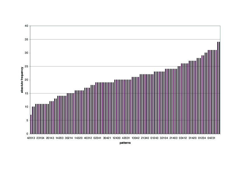
Figure 1: Histogram of pattern frequency for the whole period.

Table 8: Absolute frequency of each day in each position. Whole period: 03/01/1966–08/12/2017. Columns 2 to 6 reflect the frequency a given day is the worst return of its week, the next to worst return, etc. until the best return of its week. $Q$ is the $\chi^{2}$ statistic defined in equation 6. Hurst=0.5471.

	worst return			best return		$Q$
Mo	637	503	537	501	532	22.78967∗∗∗
Tu	557	572	475	509	597	17.94834∗∗∗
We	479	540	564	564	563	9.92989∗∗
Th	570	505	564	581	490	12.66052∗∗
Fr	467	590	570	555	528	16.74908∗∗∗
Total	2710	2710	2710	2710	2710
$Q$	36.21402∗∗∗	11.25092∗∗	11.56089∗∗	9.12177∗	11.92989∗∗
∗,∗∗,∗∗∗: significant at 10%, 5% and 1% level.

Table 9: Absolute frequency of each day in each position with shuffled data for the whole period. Columns 2 to 6 reflect the frequency a given day is the worst return of its week, the next to worst return, etc. until the best return of its week. $Q$ is the $\chi^{2}$ statistic defined in equation 6.

	worst return			best return		$Q$
Mo	506	469	501	484	480	1.91393
Tu	488	508	472	498	474	1.95082
We	513	475	491	471	490	2.24590
Th	479	491	509	482	479	1.32787
Fr	454	497	467	505	517	5.75410
Total	2440	2440	2440	2440	2440
$Q$	4.47951	2.09016	2.69672	1.49590	2.43033
∗,∗∗,∗∗∗: significant at 10%, 5% and 1% level.

Table 10: Absolute frequency of each day in each position. Subperiod 1: 03/01/1966–09/09/1977. Columns 2 to 6 reflect the frequency a given day is the worst return of its week, the next to worst return, etc. until the best return of its week. $Q$ is the $\chi^{2}$ statistic defined in equation 6. Hurst=0.5633

	worst return			best return		$Q$
Mo	182	121	105	97	105	39.37705∗∗∗
Tu	108	145	107	124	126	7.95082∗
We	108	99	120	142	141	12.21311∗∗
Th	116	119	138	132	105	5.65574
Fr	96	126	140	115	133	9.72131∗∗
Total	610	610	610	610	610
$Q$	38.55738∗∗∗	8.88525∗	9.00000∗	9.65574∗∗	8.81967∗
∗,∗∗,∗∗∗: significant at 10%, 5% and 1% level.

Table 11: Absolute frequency of each day in each position. Subperiod 2: 12/09/1977–19/05/1989.Columns 2 to 6 reflect the frequency a given day is the worst return of its week, the next to worst return, etc. until the best return of its week. $Q$ is the $\chi^{2}$ statistic defined in equation 6. Hurst=0.5168

	worst return			best return		$Q$
Mo	165	111	110	107	117	19.37705∗∗∗
Tu	138	117	111	104	140	8.60656∗
We	100	125	129	131	125	5.18033
Th	112	119	129	148	102	10.11475∗∗
Fr	95	138	131	120	126	8.90164∗
Total	610	610	610	610	610
$Q$	28.01639∗∗∗	3.44262	3.63934	10.73770∗∗	6.34426
∗,∗∗,∗∗∗: significant at 10%, 5% and 1% level.

Table 12: Absolute frequency of each day in each position. Subperiod 3: 22/05/1989–26/01/2001. Columns 2 to 6 reflect the frequency a given day is the worst return of its week, the next to worst return, etc. until the best return of its week. $Q$ is the $\chi^{2}$ statistic defined in equation 6. Hurst=0.4453

	worst return			best return		$Q$
Mo	109	105	133	126	137	6.72131
Tu	136	124	103	119	128	4.96721
We	89	141	147	125	108	18.68852∗∗∗
Th	154	117	108	123	108	11.81967∗∗
Fr	122	123	119	117	129	0.68852
Total	610	610	610	610	610
$Q$	20.31148∗∗∗	5.57377	10.75410∗∗	0.49180	5.75410
∗,∗∗,∗∗∗: significant at 10%, 5% and 1% level.

Table 13: Absolute frequency of each day in each position. Subperiod 4: 29/01/2001–05/10/2012. Columns 2 to 6 reflect the frequency a given day is the worst return of its week, the next to worst return, etc. until the best return of its week. $Q$ is the $\chi^{2}$ statistic defined in equation 6. Hurst= 0.4983

	worst return			best return		$Q$
Mo	134	106	121	128	121	3.59016
Tu	112	139	117	106	136	7.09836
We	126	115	125	115	129	1.40984
Th	131	105	121	125	128	3.40984
Fr	107	145	126	136	96	13.45902∗∗∗
Total	610	610	610	610	610
$Q$	4.63934	11.57377∗∗	0.42623	4.47541	7.85246∗
∗,∗∗,∗∗∗: significant at 10%, 5% and 1% level.

Table 14: Absolute frequency of each day in each position. Subperiod 5: 08/10/2012–08/12/2017. Columns 2 to 6 reflect the frequency a given day is the worst return of its week, the next to worst return, etc. until the best return of its week. $Q$ is the $\chi^{2}$ statistic defined in equation 6. Hurst= 0.4914

	worst return				best return	$Q$
Mo	47	60	68	43	52	7.51852
Tu.	63	47	37	56	67	10.96296∗∗
We	56	60	43	51	60	3.81481
Th	57	45	68	53	47	6.22222
Fr	47	58	54	67	44	6.18519
Total	270	270	270	270	270
$Q$	3.55556	4.03704	14.85185∗∗∗	5.62963	6.62963
∗,∗∗,∗∗∗: significant at 10%, 5% and 1% level.

In the Supplementary Material file we present the simulation and test of hypotheses for shorter time series. Additionally, we perform an exhaustive analysis of 83 stock indices with different Hurst levels. We can observe that greater Hurst-levels are associated with more significant presence of preferred patterns.

It is clear that theoretical and empirical analyses exhibit some differences. We have to acknowledge that real stock markets dynamics do no follow a pure fGn. In fact, there is not only long range dependence in financial time series, but also in volatility, as shown recently by Bariviera, (2017). Precisely, more advanced models such as the fractional normal tempered stable process presented by Kim, (2012, 2015), allow for long range dependence in both volatility and noise, and asymmetric dependence structure for the joint distribution. There are many economic variables that influence behaviors known as “stylized facts” of financial time series: volatility clustering, fat tails, asymmetric dependence, etc. For example, Kim, (2016) finds that long range dependence increases more in volatile markets, during the Lehman Brothers collapse.

We try to emphasize in this paper that, even using a simple model such as a fGn, some part of the seasonal effect is simply due to the correlation structure of data, and not only by economic reasons. This finding could be used as a starting point in further research, in order to apply prewhitening to time series previous to its analysis, in order to obtain more reliable results.

6 Conclusions

We propose a more general definition of the day-of-the-week effect. We use symbolic time series analysis in order to develop a test to detect it. According to Definition 1, this effect takes place when a pattern is much more or much less frequent than expected from the uniform distribution. The nature of the seasonal effect is reflected in a frequency matrix (Definition 2), and a $\chi^{2}$ test is performed. The new definition allows for a more general and comprehensive study on return seasonality. We would like to highlight that the methodology we use here is unique in that it is nonlinear, ordinal, requires no a priori model. Additionally, it provides statistical results in term of a probability density function. To the extent of our knowledge, no one using time series analysis has used a similar methodology before.

Both, theoretical and empirical applications show that this method could be useful to discriminate between rare and preferred patterns of a time series. We show that the so-called day-of-the-week effect is influenced not only by traders’ behavior or economic variables. It could be also be induced by the stochastic generating process of data. The findings in this paper could be taken into account in future research, aiming at the separation between the economics causes and the long-range correlation causes of this financial phenomenon.

References

- Al-Loughani and Chappell, (2001) Al-Loughani, N. and Chappell, D. (2001). Modelling the day-of-the-week effect in the kuwait stock exchange: a nonlinear garch representation. Applied Financial Economics, 11(4):353–359.
- Amigó et al., (2006) Amigó, J. M., Kocarev, L., and Szczepanski, J. (2006). Order patterns and chaos. Physics Letters A, 355(1):27 – 31.
- Amigó et al., (2007) Amigó, J. M., Zambrano, S., and Sanjuán, M. A. F. (2007). True and false forbidden patterns in deterministic and random dynamics. EPL (Europhysics Letters), 79(5):50001.
- Amigó et al., (2008) Amigó, J. M., Zambrano, S., and Sanjuán, M. A. F. (2008). Combinatorial detection of determinism in noisy time series. EPL (Europhysics Letters), 83(6):60005.
- Bandt and Pompe, (1993) Bandt, C. and Pompe, B. (1993). The entropy profile - a function describing statistical dependences. Journal of Statistical Physics, 70(3-4):967–983.
- Bandt and Pompe, (2002) Bandt, C. and Pompe, B. (2002). Permutation entropy: A natural complexity measure for time series. Phys. Rev. Lett., 88:174102.
- Bariviera, (2011) Bariviera, A. F. (2011). The influence of liquidity on informational efficiency: The case of the thai stock market. Physica A: Statistical Mechanics and its Applications, 390(23-24):4426–4432.
- Bariviera, (2017) Bariviera, A. F. (2017). The inefficiency of bitcoin revisited: A dynamic approach. Economics Letters, 161(Supplement C):1 – 4.
- Bariviera and de Andrés Sánchez, (2005) Bariviera, A. F. and de Andrés Sánchez, J. (2005). ¿existe estacionalidad diaria en el mercado de bonos y obligaciones del estado? evidencia empírica en el período 1998-2003. Análisis Financiero, 98:16–21.
- Bariviera et al., (2012) Bariviera, A. F., Guercio, M. B., and Martinez, L. B. (2012). A comparative analysis of the informational efficiency of the fixed income market in seven european countries. Economics Letters, 116(3):426–428.
- Blume and Friend, (1973) Blume, M. E. and Friend, I. (1973). A new look at the capital asset pricing model. The Journal of Finance, 28(1):19–33.
- (12) Cajueiro, D. O. and Tabak, B. M. (2004a). Evidence of long range dependence in asian equity markets: the role of liquidity and market restrictions. Physica A: Statistical Mechanics and its Applications, 342(3-4):656–664.
- (13) Cajueiro, D. O. and Tabak, B. M. (2004b). The hurst exponent over time: testing the assertion that emerging markets are becoming more efficient. Physica A: Statistical and Theoretical Physics, 336(3-4):521–537.
- Carpi et al., (2010) Carpi, L. C., Saco, P. M., and Rosso, O. (2010). Missing ordinal patterns in correlated noises. Physica A: Statistical Mechanics and its Applications, 389(10):2020 – 2029.
- Cross, (1973) Cross, F. (1973). The behavior of stock prices on fridays and mondays. Financial Analysts Journal, 29(6):67–69.
- Fama, (1970) Fama, E. F. (1970). Efficient capital markets: A review of theory and empirical work. The Journal of Finance, 25(2, Papers and Proceedings of the Twenty-Eighth Annual Meeting of the American Finance Association New York, N.Y. December, 28-30, 1969):383–417.
- Fama and MacBeth, (1973) Fama, E. F. and MacBeth, J. D. (1973). Risk, return, and equilibrium: Empirical tests. Journal of Political Economy, 81(3):607–636.
- Fernández Loureiro, (2011) Fernández Loureiro, E. (2011). Estadística no paramétrica: a modo de introducción. Ediciones Cooperativas, Buenos Aires.
- Fields, (1931) Fields, M. J. (1931). Stock prices: A problem in verification. The Journal of Business of the University of Chicago, 4(4):415–418.
- Fields, (1934) Fields, M. J. (1934). Security prices and stock exchange holidays in relation to short selling. The Journal of Business of the University of Chicago, 7(4):328–338.
- French, (1980) French, K. R. (1980). Stock returns and the weekend effect. Journal of Financial Economics, 8(1):55–69.
- Gibbons and Hess, (1981) Gibbons, M. R. and Hess, P. (1981). Day of the week effects and asset returns. The Journal of Business, 54(4):579–596.
- Hurst, (1951) Hurst, H. E. (1951). Long-term storage capacity of reservoirs. Transactions of the American Society of Civil Engineers, 116:770–808.
- Keim and Ziemba, (2000) Keim, D. B. and Ziemba, W. T., editors (2000). Security Market Imperfections in Worldwide Equity Markets. Cambridge University Press, Cambridge.
- Keloharju et al., (2016) Keloharju, M., Linnainmaa, J. T., and Nyberg, P. (2016). Return seasonalities. The Journal of Finance, 71(4):1557–1590.
- Kim, (2012) Kim, Y. S. (2012). The fractional multivariate normal tempered stable process. Applied Mathematics Letters, 25(12):2396 – 2401.
- Kim, (2015) Kim, Y. S. (2015). Multivariate tempered stable model with long-range dependence and time-varying volatility. Frontiers in Applied Mathematics and Statistics, 1:1.
- Kim, (2016) Kim, Y. S. (2016). Long-range dependence in the risk-neutral measure for the market on lehman brothers collapse. Applied Mathematical Finance, 23(4):309–322.
- Koh and K.A., (2000) Koh, S.-K. and K.A., W. (2000). Anomalies in asian emerging stock markets. In Keim, D. B. and Ziemba, W. T., editors, Security Market Imperfections in Worldwide Equity Markets, pages 353–359. Cambridge University Press, Cambridge.
- Kuhn, (1968) Kuhn, T. S. (1968). The Structure of scientific revolutions. University of Chicago, Chicago.
- Lauterbach and Ungar, (1992) Lauterbach, B. and Ungar, M. (1992). Calendar anomalies: some perspectives from the behaviour of the israeli stock market. Applied Financial Economics, 2(1):57–60.
- LeRoy, (1989) LeRoy, S. F. (1989). Efficient capital markets and martingales. Journal of Economic Literature, 27(4):1583–1621.
- Lintner, (1965) Lintner, J. (1965). The valuation of risk assets and the selection of risky investments in stock portfolios and capital budgets. The review of economics and statistics, 47(1):13–37.
- Mandelbrot, (1972) Mandelbrot, B. B. (1972). Statistical methodology for nonperiodic cycles: From the covariance to rs analysis. In Annals of Economic and Social Measurement, Volume 1, number 3, NBER Chapters, pages 259–290. National Bureau of Economic Research.
- Mandelbrot and Wallis, (1968) Mandelbrot, B. B. and Wallis, J. R. (1968). Noah, joseph, and operational hydrology. Water Resources Research, 4(5):909–918.
- Mossin, (1966) Mossin, J. (1966). Equilibrium in a capital asset market. Econometrica, 34(4):768–783.
- Parlitz et al., (2012) Parlitz, U., Berg, S., Luther, S., Schirdewan, A., Kurths, J., and Wessel, N. (2012). Classifying cardiac biosignals using ordinal pattern statistics and symbolic dynamics. Computers in Biology and Medicine, 42(3):319–327.
- Rogalski, (1984) Rogalski, R. J. (1984). New findings regarding day-of-the-week returns over trading and non-trading periods: A note. The Journal of Finance, 39(5):1603–1614.
- Rosso et al., (2012) Rosso, O., Carpi, L., Saco, P., Ravetti, M., Larrondo, H., and Plastino, A. (2012). The amigó paradigm of forbidden/missing patterns: a detailed analysis. The European Physical Journal B, 85:1–12.
- Saco et al., (2010) Saco, P. M., Carpi, L. C., Figliola, A., Serrano, E., and Rosso, O. A. (2010). Entropy analysis of the dynamics of el niño/southern oscillation during the holocene. Physica A: Statistical Mechanics and its Applications, 389(21):5022–5027.
- Sharpe, (1964) Sharpe, W. F. (1964). Capital asset prices: A theory of market equilibrium under conditions of risk. The Journal of Finance, 19(3):425–442.
- Zanin, (2008) Zanin, M. (2008). Forbidden patterns in financial time series. Chaos, 18(1):936–947.
- Zhang et al., (2017) Zhang, J., Lai, Y., and Lin, J. (2017). The day-of-the-week effects of stock markets in different countries. Finance Research Letters, 20(Supplement C):47 – 62.
- Ziemba, (2012) Ziemba, W. T., editor (2012). Calendar Anomalies and Arbitrage. World Scientific, Singapore.
- Zunino et al., (2012) Zunino, L., Bariviera, A. F., Guercio, M. B., Martinez, L. B., and Rosso, O. A. (2012). On the efficiency of sovereign bond markets. Physica A: Statistical Mechanics and its Applications, 391(18):4342–4349.
- Zunino et al., (2011) Zunino, L., Tabak, B. M., Serinaldi, F., Zanin, M., Pérez, D. G., and Rosso, O. A. (2011). Commodity predictability analysis with a permutation information theory approach. Physica A: Statistical Mechanics and its Applications, 390(5):876–890.
- Zunino et al., (2010) Zunino, L., Zanin, M., Tabak, B. M., Pérez, D. G., and Rosso, O. A. (2010). Complexity-entropy causality plane: A useful approach to quantify the stock market inefficiency. Physica A: Statistical Mechanics and its Applications, 389(9):1891–1901.