Anomalous Hall effect in 2D Dirac materials

Abstract

We present a unified theory of charge carrier transport in 2D Dirac systems with broken mirror inversion and time-reversal symmetries (e.g., as realized in ferromagnetic graphene). We find that the entanglement between spin and pseudospin SU(2) degrees of freedom stemming from spin–orbit effects leads to a distinctive gate voltage dependence (change of sign) of the anomalous Hall conductivity approaching the topological gap, which remains robust against impurity scattering and thus is a smoking gun for magnetized 2D Dirac fermions. Furthermore, we unveil a robust skew scattering mechanism, modulated by the spin texture of the energy bands, which causes a net spin accumulation at the sample boundaries even for spin-transparent disorder. The newly unveiled extrinsic spin Hall effect is readily tunable by a gate voltage and opens novel opportunities for the control of spin currents in 2D ferromagnetic materials.

Ferromagnetic order in two-dimensional (2D) crystals is of great significance for fundamental studies and applications in spintronics. Recent experiments have revealed that intrinsic ferromagnetism occurs in 2D crystals of Cr₂Ge₂Te₆ Cr2Ge2Te6_Gong_17 and CrI₃ CrI3_Huang_17 , while graphene and group-VI dichalcogenide monolayers acquire large exchange splitting when integrated with nanomagnets Ferr_G_YIG_Swartz12 ; Ferr_G_YIG_Wang15 ; AHE_G_Tang_18 ; Ferr_G_YIG_Leutnantsmeyer_17 ; Ferro_Gr_EuS_Wu17 ; Ferro_Gr_BiFeO3_Wu17 ; Ferro_vdW_mat .

Different from bulk compounds, the electronic states of atomically thin layers can be dramatically affected by short-range magnetic interactions, opening up a new arena for studies of emergent spin-dependent phenomena MEC_Gr_Theory_Haugen08 ; MEC_Gr_Theory_QAHE_Sun_10 ; MEC_Gr_Theory_Sun11 ; MEC_Gr_Theory_Yang13 ; MEC_Gr_Theory_Marchenko15 . In this regard, graphene and other 2D Dirac materials with multiple internal degrees of freedom offer particularly promising perspectives. The anomalous Hall effect (AHE) recently observed in graphene/yttrium iron garnet heterostructures indicates that interface-induced magnetic exchange coupling (MEC) is accompanied by sizable Bychov-Rashba effect Ferr_G_YIG_Wang15 ; AHE_G_Tang_18 . The breaking of inversion symmetry in a honeycomb layer couples different SU(2) subspaces (spin and sublattice) GRashba_09 and can drive the ferromagnetic 2D Dirac system through a topological phase transition to a Chern insulator when the chemical potential is tuned inside the gap MEC_Gr_Theory_QAHE_Sun_10 ; Chen_11 ; QAHE_G_2 . This system is predicted to exhibit the quantum anomalous Hall effect (QAHE), with transverse conductivity $\sigma_{\text{AH}}=2\,e^{2}/h$ MEC_Gr_Theory_QAHE_Sun_10 . However, much less is known about the non-quantized regime at finite carrier density. The latter is the current experimental accessible regime Ferr_G_YIG_Wang15 ; AHE_G_Tang_18 . Beyond the non-quantized part of the intrinsic contribution, the presence of a Fermi surface makes the transverse (anomalous Hall) conductivity depend nontrivially on spin-dependent scattering due to pseudospin-spin coupling ferreira2014 ; Tuan16 ; milletari16 ; ASP_Huang_16 . Moreover, in ultraclean heterostructures, the MEC and spin–orbit coupling (SOC) energy scales can easily reach the disorder-induced broadening Zollner_PRB2016 ; Gmitra_PRB2016 ; Wang_NatComm2015 , thus questioning the use of standard approaches where SOC is treated as a weak perturbation.

In this Letter, we report an accurate theoretical study of charge and spin transport in magnetized 2D Dirac systems by treating the effects of strong MEC and SOC nonperturbatively in the presence of dilute random impurities. Our theory is valid for both weak (Born) and strong (unitary) potential scattering and accounts for intervalley processes from point defects. We find that the out-of-plane component of the noncollinear spin texture $\mathbf{S}_{\mu\nu\mathbf{k}}$ [with $\mu(\nu)=\pm 1$ pseudospin (spin chirality); Fig. 1] activates a robust skew scattering mechanism, which determines the behavior of leading Fermi surface contributions to the transverse transport coefficients. The $\mathbf{k}$ modulation of the spin polarization manifests into a ubiquitous change of sign in the charge Hall conductivity as the Fermi level approaches the majority spin band edge, which, as we argue below, is a forerunner of the elusive QAHE Ferr_G_YIG_Wang15 ; AHE_G_Tang_18 ; Leutenantsmeyer_16 . Second, we predict that scattered electron waves with opposite polarization (e.g., from within the ’Mexican hat’ with $S_{\mathbf{k}_{\pm}}^{z}\gtrless 0$; Fig. 1) have different transverse cross section leading to net spin Hall current in the bulk SHE_RMP_2015 . Such a spin Hall effect (SHE) in a 2D Dirac system with broken time reversal symmetry can be seen as the reciprocal of the inverse spin Hall effect discovered recently in ferromagnets Miao_PRL2013 ; Das_PRBR2017 ; Iihama_NatElet2018 . The common stem of AHE and SHE implies the change of sign reveals likewise in the spin Hall response, unveiling the possibility of reversing the spin accumulation at the sample boundaries by gate voltage. The sign-change feature is found to be preserved when adding the Berry curvature-dependent contributions to the AHE and SHE over a wide range of parameters in samples with high mobility.

Model.—The low-energy Hamiltonian reads (we use natural units $e\equiv 1\equiv\hbar$, unless stated otherwise)

$$H=v\,\tau_{z}\,\boldsymbol{\Sigma}\cdot\mathbf{p}+\text{$\delta$}\,s_{z}+\lambda\,\tau_{z}\left(\Sigma_{x}s_{y}-\Sigma_{y}s_{x}\right)+V(\mathbf{x})\,,$$ (1)

where $v$ is the Fermi velocity of massless Dirac fermions, $\delta$ ($\lambda$) is the MEC (Bychov-Rashba) energy scale, and $V(\mathbf{x})$ is a disorder potential describing impurity scattering. Here, $\left\{\boldsymbol{\tau},\boldsymbol{\Sigma},\mathbf{s}\right\}$ are Pauli matrices defined on valley, pseudospin and spin spaces, respectively, and $\mathbf{p}=-i\boldsymbol{\nabla}$ is the 2D kinematic momentum operator for states near the $K$ ($K^{\prime}$) point ($\tau_{z}=\pm 1$). This model describes magnetized graphene with $C_{6v}$ point group symmetry Ferr_G_YIG_Wang15 ; AHE_G_Tang_18 and can be easily extended to other ferromagnetic 2D materials, such as MoTe₂/EuO Qi_MoTe2_2015 ; Cheng_16 ; Yao_PRB2017 . We consider (nonmagnetic) matrix disorder with $V(\mathbf{x})=\sum_{i}\left(u_{0}1+u_{x}\tau_{x}\right)\delta(\mathbf{x}-\mathbf{x}_{i})$, where $\{\mathbf{x}_{i}\}_{i=1...N}$ are random impurity positions and $u_{0(x)}$ parameterizes the intravalley (intervalley) scattering strength G_Review ; ResonantScatt_G . This choice allows us to interpolate between “smooth” potentials in clean samples ($|u_{x}|\ll|u_{0}|$) and the “sharp defect” limit of enhanced backscattering processes ($u_{x}\approx u_{0}$). The energy-momentum dispersion relation associated to clean system $H_{0}=H-V(\text{{x}})$ reads

$$\epsilon_{\mu\nu}(\mathbf{k})=\mu\sqrt{v^{2}k^{2}+M_{\nu}^{2}\left(k\right)}\,,$$ (2)

where $M_{\nu}(k)=\sqrt{2\lambda^{2}+\text{$\delta^{2}$}+2\nu\sqrt{\lambda^{4}+v^{2}k^{2}(\lambda^{2}+\text{$\delta^{2}$})}}$ is the SOC mass and $k=|\mathbf{k}|$ is the wavevector measured from a Dirac point. Indices $\{\mu,\nu\}=\pm 1$ define the carrier polarity and the spin winding direction (Fig. 1).

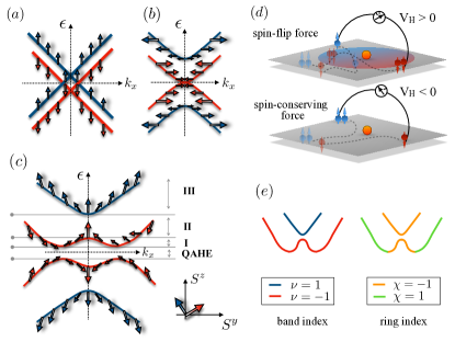
Figure 1: (a-c) Energy bands and spin texture in systems with (a) MEC (b) SOC and (c) MEC and SOC. For visualization purposes, the bands are plotted along $\hat{k}_{x}$ (spins lie only in the $yz$ plane). (d) Behavior of Hall conductivity due to competing spin-Lorentz forces. The elastic scattering channel dominates in regime II and III. (e) Band classification using band (ring) index $\nu=\pm 1$ ($\chi=\pm 1$).

In the absence of SOC, the Dirac cones are shifted vertically, resulting in mixed electron–hole states near the Dirac point. For $\lambda\neq 0,\,\text{$\delta$}=0$ (no MEC), the spectrum admits a spin-gap or pseudogap region, within which the spin and momentum of quasiparticles are locked at right angles (Bychov-Rashba spin texture) GRashba_09 ; offidani17 . The combination of SOC and MEC opens a gap and splits the Dirac spectrum into 3 branches: regions I and III, defined by $|\lambda\text{$\text{$\delta$}$|/$\sqrt{\lambda^{2}+\text{$\text{$\delta$}^{2}$}}$}\equiv\textrm{$\epsilon$}_{\textrm{I}}<|\epsilon|<\epsilon_{\textrm{II}}=|\text{$\delta$|}$ and $|\epsilon|>\sqrt{4\lambda^{2}+\text{$\text{$\delta$}^{2}$}}\equiv\epsilon_{\textrm{III}}$; those energy regimes are characterized by a non-simply connected Fermi surface allowing for scattering between states with different Fermi momenta; and region II, $\epsilon_{\textrm{II}}<|\epsilon|<\epsilon_{\textrm{III}}$, with only one band intersecting the Fermi level. For brevity, all functions are projected onto valley $\tau_{z}=1$ ($K$ point). The Bloch eigenstates read as

$$|\psi_{\mu\nu\mathbf{k}}\left(\mathbf{x}\right)\rangle=\left(\begin{array}[]{c}e_{\,}^{-\imath\phi_{\mathbf{k}}}\\ \imath\frac{\left(\epsilon_{\mu\nu}-\text{$\text{$\delta$}$}\right)^{2^{\,}}-v^{2}k^{2}}{2\,v\,k\,\lambda_{\,}}\\ \frac{\epsilon_{\mu\nu}-\text{$\text{$\delta$}^{\,}$}}{vk_{\,}}\\ \imath\frac{\left(\epsilon_{\mu\nu}-\text{$\text{$\delta$}$}\right)^{2^{\,}}-v^{2}k^{2}}{2\,\lambda\left(\epsilon_{\mu\nu}+\text{$\text{$\delta$}$}\right)}e^{\imath\phi_{\mathbf{k}}}\end{array}\right)e^{\imath\mathbf{k}\cdot\mathbf{x}}\,,$$ (3)

where $\phi_{\mathbf{k}}$ is the wavevector polar angle. The noncoplanar spin texture in momentum space highlights the competition between different interactions: while the Bychov-Rashba effect favors in-plane alignment, the exchange interaction tilts the spins out of the plane, leading to a noncoplanar band polarization [Fig. 1 (c)]. The pronounced effects of symmetry breaking on the spin texture has been highlighted in other systems, e.g. surface states of Bi thin films Takayama_2011PRL . We underline here its impact on relativistic transport: as shown below, the out-of-plane spin texture $S_{\mu\nu\mathbf{k}}^{z}\equiv\frac{1}{2}\langle s_{z}\rangle_{\mu\nu\mathbf{k}}$ modulates intrinsic and extrinsic transport contributions; even if the electronic states are not fully spin polarized, it will prove useful to refer to effective spin-up ($S^{z}>0$) and spin-down ($S^{z}<0)$ states. We focus on positive energies, $\epsilon>0$, and also $\lambda,\delta>0$, thus fixing $\mu=1$ and omitting this index from the expressions.

Spin texture-driven skew scattering.— To assess the dominant extrinsic transport contributions in the metallic regime ($\epsilon>\epsilon_{\textrm{I}}$), we solve the Boltzmann transport equations (BTEs) for a spatially homogeneous system. The formalism allows for the inclusion of a nonquantizing magnetic field and, more importantly, for a transparent physical interpretation of the scattering processes. For a controlled quantum diagrammatic treatment at the $T$-matrix level, we refer the reader to the supplementary material (SM) supplemMat , where quantum side jump corrections are shown to be subleading for typical (dilute) impurity concentrations. The BTEs read as

$$\partial_{t}f_{\mathbf{k}_{\chi}}-e\left(\boldsymbol{\mathcal{E}}+\mathbf{v}\times\boldsymbol{\mathcal{B}}\right)\cdot\nabla_{\mathbf{k}}f_{\mathbf{k}_{\chi}}=2\pi n_{i}\sum_{\chi^{\prime}=\pm 1}\int\frac{Sd^{2}\mathbf{k}^{\prime}}{(2\pi)^{2}}\left(f_{\mathbf{k}_{\chi^{\prime}}^{\prime}}\mathcal{T}_{\mathbf{k}_{\chi^{\prime}}^{\prime}\mathbf{k}_{\chi}}-f_{\mathbf{k}_{\chi}}\mathcal{T}_{\mathbf{k}_{\chi}\mathbf{k}_{\chi^{\prime}}^{\prime}}\right)\,\delta(\epsilon_{\mathbf{k}_{\chi}}-\epsilon_{\mathbf{k}_{\chi^{\prime}}^{\prime}})\,,$$ (4)

where $f_{\mathbf{k}_{\chi}}=f_{\mathbf{k}_{\chi}}^{0}+\delta f_{\mathbf{k}_{\chi}}$ is the sum of the Fermi-Dirac distribution function and $\delta f_{\mathbf{k}_{\chi}}$, the deviation from equilibrium. Moreover, $\boldsymbol{\mathcal{E}},\boldsymbol{\mathcal{B}}$ are external DC fields, $e$ is the elementary charge and $S$ is the area. The right-hand side is the collision term describing single impurity scattering and $n_{i}$ is the impurity areal density. Subscripts $\chi,\chi^{\prime}=\pm 1$ are ring indices for the outer/inner Fermi surfaces associated with momenta $k_{\pm}=v^{-1}\{\epsilon^{2}+\text{$\delta^{2}$}\pm[\epsilon^{2}\lambda^{2}+(\epsilon^{2}-\lambda^{2})\delta^{2}]^{1/2}\}^{1/2}$; Fig. 1(d) CommentRingIndex . Accounting for possible scattering resonances due to the Dirac spectrum ferreira2014 , transition rates are evaluated by means of the $T$-matrix approach i.e., $\mathcal{T}_{\mathbf{k}\mathbf{k}^{\prime}}=\left|\langle\mathbf{k}^{\prime}|t|\mathbf{k}\rangle\right|^{2}$, where $t=\mathcal{V}/\left(1-g_{0}\,\mathcal{V}\right)$ with $\mathcal{V}=u_{0}+\tau_{x}u_{x}$ and $g_{0}=\int d^{2}\mathbf{k}/(4\pi^{2})\,(\epsilon-H_{0\mathbf{k}}+\imath\,0^{+})^{-1}$ is the integrated propagator. We start by considering $u_{x}=0$, for which electrons undergo intra- and inter-ring scattering processes in the same valley (see supplemMat for a graphical visualization). Exploiting the Fermi surface isotropy, and momentarily setting $\boldsymbol{\mathcal{B}}=0$, the exact solution to the linearized BTEs ($\nabla_{\mathbf{k}}f_{\mathbf{k}_{\chi}}\rightarrow\nabla_{\mathbf{k}}f_{\mathbf{k}_{\chi}}^{0}$) is

$$\delta f_{\mathbf{k}_{\chi}} =-e\left(\frac{\partial f_{\mathbf{k}_{\chi}}^{0}}{\partial\epsilon}\right)\,\mathbf{v}_{\mathbf{k}_{\chi}}\cdot\left(\tau_{\chi}^{\parallel}\,\boldsymbol{\mathcal{E}}+\tau_{\chi}^{\perp}\,\hat{z}\times\boldsymbol{\mathcal{E}}\right)\,,$$ (5)

with $\mathbf{v}_{\mathbf{k}_{\chi}}=\nabla_{\mathbf{k}}\epsilon_{\chi}(\mathbf{k})$. In the above, $\tau_{\chi}^{\varsigma}=\tau_{\chi}^{\varsigma}(\epsilon,\lambda,\text{$\delta$},u_{0},n_{i})$ are the longitudinal ($\varsigma=\parallel$) and transverse ($\varsigma=\perp$) transport times given by

$$\boldsymbol{\tau}^{\parallel} =-2\left(\hat{\Lambda}+\hat{\Upsilon}\hat{\Lambda}^{-1}\hat{\Upsilon}\right)^{-1}\boldsymbol{1}\,,\,\,\,\boldsymbol{\tau}^{\perp}=\hat{\Lambda}^{-1}\hat{\Upsilon}\,\boldsymbol{\tau}^{\parallel}\,,$$ (6)

where $\boldsymbol{\tau}^{\varsigma}=(\tau_{\chi}^{\varsigma},\tau_{\bar{\chi}}^{\varsigma})^{\text{t}}$, $\hat{\Lambda}=((\Lambda_{\chi}^{-},\Lambda_{\chi}^{+})^{\text{t}},(\Lambda_{\bar{\chi}}^{-},-\Lambda_{\bar{\chi}}^{+})^{\text{t}})$, $\boldsymbol{1}=(1,0)^{\text{t}}$ and $\bar{\chi}\equiv-\chi$ ($\hat{\Upsilon}$ is obtained from $\hat{\Lambda}$ via the substitution $\Lambda_{\chi}^{\pm}\to\Upsilon_{\chi}^{\mp}$). The kernels $\Lambda_{\chi}^{\pm}$ and $\Upsilon_{\chi}^{\pm}$ are cumbersome functions of symmetric and skew cross sections defined by $\boldsymbol{\Gamma}_{\chi\chi^{\prime}}=\frac{n_{i}}{2\pi}\int Sd^{2}\text{{k}}^{\prime}\,\mathcal{T}_{\mathbf{k}_{\chi^{\prime}}^{\prime}\mathbf{k}_{\chi}}\,\left\{1,\cos\phi,\sin\phi\right\}^{\textrm{t}}$ with $\phi=\phi_{\text{{k}}^{\prime}}-\phi_{\text{{k}}}$ supplemMat . Considering the two valleys, the general solution involves 16 cross sections. The exact form of the kernels is essential to correctly determine the energy dependence of the conductivity tensor. As shown in SM supplemMat , including a magnetic field $\boldsymbol{\mathcal{B}}=\mathcal{B}\,\hat{z}$ only requires the substitution $\Gamma_{\chi\chi}^{\text{sin}}\to\Gamma_{\chi\chi}^{\text{sin}}+\omega_{\chi}$, where $\omega_{\chi}=k_{\chi}v_{\chi}^{-1}\mathcal{B}$ is the cyclotron frequency associated with the ring states. At $T=0$, accounting for the valley degeneracy, we obtain the transverse response functions

$$\sigma_{\perp}^{c,s}(\mathcal{B},\epsilon)=\frac{-e}{h}\sum_{\chi=\pm 1}k_{\chi}(\epsilon)\,\langle J_{c,s}(\epsilon)\rangle_{\chi}\,\tau_{\chi}^{\perp}(\epsilon,\mathcal{B})\,,$$ (7)

where $\langle J_{c,s}(\epsilon)\rangle_{\chi}=-e\,\langle\{1,s_{z}/2\}\,\boldsymbol{\Sigma}\cdot|\hat{z}\times\boldsymbol{\hat{\mathcal{E}}}|\rangle_{\chi}$ denotes the equilibrium transverse charge (spin) current of planewave states in the $\chi$ ring. The skew cross sections (and hence $\tau_{\chi}^{\perp}$) are found to be nonzero (except for isolated points) and thus, in the dilute regime, one has $\sigma_{\perp}^{c,s}\propto n_{i}^{-1}$, which is a signature of skew scattering milletari16 . As discussed below, the energy dependence of the skew cross sections is very marked, reflecting the out-of-plane spin texture of conducting electrons. For simplicity, in what follows, we work at saturation field $\mathcal{B}\geq\mathcal{B}_{\text{sat}}$ such that the transverse responses coincide with their “anomalous” parts, that is, $\left.\sigma_{\text{AH(SH)}}(\mathcal{B}_{\text{sat}},\epsilon)\right|_{\delta}\simeq\left.\sigma_{\perp}(0,\epsilon)\right|_{\delta_{\textrm{sat}}}$, where $\delta_{\textrm{sat}}=\delta(M_{z}(\mathcal{B}_{\text{sat}}))$ and $M_{z}$ is the magnetization.

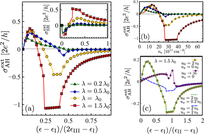
Figure 2: Energy dependence of AHE and SHE. (a) $\sigma_{\perp}^{c,s}(\epsilon)$ is the result of the competing effective spin Lorentz forces as discussed in the main text [see also Fig. (1)(e)]. The change of sign is more prominent for large SOC. (b) $\sigma_{\perp}^{c}(n_{e})$ where $n_{e}=\pi\{k_{+}^{2}-k_{-}^{2},\,k_{+}^{2},\,k_{+}^{2}+k_{-}^{2}\}$, respectively, in regions I, II, and III. (c) While less evident in the unitary limit, the change of sign is robust across all scattering regimes. $\delta=30$ meV, $\lambda_{0}=\delta/3$, $v_{0}=u_{0}=1\,\textrm{eV}\cdot\textrm{nm}^{2},\,u_{x}=0$ and $n_{0}=10^{12}\text{cm}^{-2}$.

The change of sign.—Focusing on the regime $\lambda\lesssim\delta$, we show how, approaching low carrier density, electrons undergoing spin-conserving and spin-flip scattering processes determine a change of sign in $\sigma_{\perp}^{c,s}$. For the sake of illustration, we assume weak scatterers $|g_{0}u_{0}|\ll 1$ and restrict the analysis to intraring transitions within the outer ring: $\mathbf{k}_{+}\to\mathbf{k}_{+}^{\prime}$ (see additional discussions supplemMat ). A first scenario for the change of sign is as follows. First, we note that as $k$ is increased from $k=0$, electron states in the lower band $\nu=-1$ progressively change their spin orientation from effective spin-up to -down states (see Fig. 1). Starting from $\epsilon_{\text{I}}$, varying $\epsilon$ instead, it can be verified that the same occurs within the outer ring, such that by tuning $\epsilon$ one can switch between states with opposite spin polarization. As effective up/down states are associated with an opposite effective spin Lorentz force (i.e., skew cross sections with opposite signs), this also means conducting electrons can be selectively deflected towards opposite boundaries of the system. The associated anomalous Hall (AH) voltage and SHE spin accumulation will then display the characteristic change of sign [Fig. 2(a)].

A second scenario involves the spin-flip force and does not require changing the polarization of carriers. Instead, what changes when varying $\epsilon$ is the ratio of spin-flip to elastic skew cross sections. This also produces a change of sign as depicted in Fig. 1(e); the fate of the transverse conductivity will depend ultimately on the competition between the two effective spin Lorentz forces (see SM supplemMat ). The change of sign in $\sigma_{\perp}^{c,s}$ is a persistent feature as long as SOC and MEC are comparable [Fig. 2(a)]. In that case, the noncollinear spin texture is well developed, such that, on one hand, it is possible to interchange between effective spin-up and -down states $"S"="\uparrow,\downarrow"=-"\bar{S}"$ using a gate voltage, and, on the other, both spin-conserving $\langle"S"|V(\text{{x}})|"S"\rangle$ and spin-flip $\langle"\bar{S}"|V(\text{{x}})|"S"\rangle$ scattering matrix elements are non-zero. Asymptotically, $\epsilon\gg\delta,\lambda$, the AH signal must vanish due to the opposite spin orientation of electron states belonging to $\nu=\pm 1$ bands, which produce vanishing small total magnetization $S^{z}(\epsilon)=\sum_{\chi}S_{\chi}^{z}\ll 1$. In comparison, the staggered field experienced by charge carriers $S_{\textrm{stag}}^{z}(\epsilon)=\sum_{\chi}\chi S_{\chi}^{z}$ has slower asymptotic decay (for $\lambda\lesssim\delta$), implying that the SHE is more robust than the AHE.

Approaching the QAHE.—The system realizes the QAHE provided the gap remains robust against disorder, $\sigma_{\perp}^{c}(\epsilon<\epsilon_{\text{I}})=2e^{2}/h,\,\,\sigma_{\perp}^{s}(\epsilon<\epsilon_{\text{I}})=0$. In the metallic regime, the Berry curvature of occupied states also provide a (nonquantized) intrinsic contribution to the transverse conductivity. Below, we discuss how robust is the change of sign to the inclusion of other factors and also how the quantized region is approached. First, consider that in the strong scattering limit, $|g_{0}u_{0}|\gg 1$, the rate of inter-ring transitions increases and the one-ring scenario presented above might break down. However, as shown in Fig. 2(c) the change of sign is still visible. In real samples, structural defects and short-range impurities, such as hydrocarbons Resonant_Scatt_Ni_10 , induce scattering between inequivalent valleys, thereby opening the backscattering channel G_Review . In fact, spin precession measurements in graphene with interface-induced SOC indicate that the in-plane spin dynamics is sensitive to intervalley scattering Benitez_17 ; Cummings_17 ; Ghiasi_17 . To determine the impact of intervalley processes on DC transport, we solved the BTEs for arbitrary ratio $u_{x}/u_{0}$. Figure 2(c) shows the AH conductivity for selected values of $u_{x}$ (dashed lines). $\sigma_{\perp}^{c}$ is strongly impacted showing a 50% reduction when intra- and intervalley scattering processes are equally probable ($u_{x}=u_{0}$). However, the sign change in $\sigma_{\perp}$, approaching the majority spin band edge $\epsilon\approx\epsilon_{\textrm{II}}$ is still clearly visible. Further analysis are given in SM supplemMat , where we also analyze the impact of thermal fluctuations, concluding that the features described above are persistent up to $k_{\text{B}}T\approx k_{\text{B}}T_{\text{room}}/2\simeq 12\,\text{meV}$ for $\lambda\approx\delta=30$ meV. A thorough numerical analysis in the strong SOC regime provides an estimation for $\epsilon_{0}$ defined as $\sigma_{\perp}(\epsilon_{0})=0$,

$$\epsilon_{0}=a\,\epsilon_{\text{I}}+b\,\epsilon_{\text{III}}\,,$$ (8)

with $a\simeq 0.3$–0.4 and $b\simeq 0.6$–0.8. This relation shows that the knowledge of $\delta$ (e.g., from the Curie temperature Ferr_G_YIG_Wang15 ) allows to estimate the SOC strength directly from the gate voltage dependence of the AH resistance. The values $\sigma_{\perp}\approx 0.1-1$ ($e^{2}/h$) are compatible with the measurements in Refs. Ferr_G_YIG_Wang15 ; AHE_G_Tang_18 , for a reasonable choice of parameters, $0\leq\lambda,\delta\leq 30\,\text{meV}$ in the dirty regime with $n_{i}=10^{12}\,\text{cm}^{2}$ and $u_{0}\sim(0.1,1)\,\text{eV}\cdot\textrm{nm}^{2}$. In high mobility samples, our theory predicts that the robust skew scattering contribution with $\sigma_{\perp}\propto n_{i}^{-1}$ results in much larger values $\sigma_{\perp}\approx 10-100$ ($e^{2}/h$).

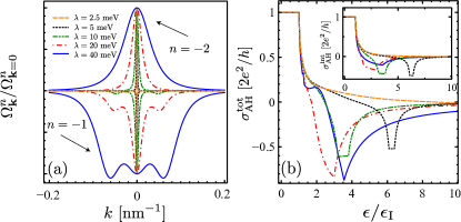
Figure 3: Intrinsic contribution and total AH conductivity at selected SOC values. (a) The Berry curvatures of hole bands $n=-1,-2$. Note that $\Omega_{n=-1}(\mathbf{k})$ develops additional “hot spots” as SOC is increased. (b) The total $\sigma_{\perp}^{\text{tot}}=\sigma_{\perp}^{\text{}}+\sigma_{\perp}^{\text{int}}$; same legend as in (a). (b) Adding the intrinsic contribution (inset) to $\sigma_{\perp}$ leaves the estimate for $\epsilon_{0}$ virtually unaffected [Eq. (8)]. Parameters: $u_{0}=10\text{ {eV}$\cdot\textrm{nm}^{2}$},$ $n_{i}=10^{12}\text{ cm}^{-2}$ and $\delta=30\text{ meV}$.

Intrinsic contribution and total AH conductivity.—We now report our results for the intrinsic contribution. Previous studies—where the topological nature of the model was also firstly pointed out MEC_Gr_Theory_QAHE_Sun_10 —tackled the problem numerically, also with a focus in the regime $\text{$\delta$}\gg\lambda$. We go beyond this limitation performing an exact analytic evaluation of the intrinsic AH conductivity. Starting from the chiral eigenstates of Eq. (3), we obtain the Berry curvature of the bands as $\Omega_{\mathbf{k}}^{n}=\left(\nabla_{\mathbf{k}}\times\boldsymbol{\mathcal{A}}_{\mathbf{k}}^{n}\right)_{z}$, where $\boldsymbol{\mathcal{A}}_{\mathbf{k}}^{n}=-i\langle n\mathbf{k}|\nabla_{\mathbf{k}}|n\mathbf{k}\rangle$ and $n\equiv(\mu,\nu)$ is a combined band index CommentIndex . The transverse conductivity is obtained via integration of the Berry curvatures TKNNFormula , $\sigma_{\perp}^{\textrm{int}}=\sum_{n}\sum_{\mathbf{k}}\Omega_{\mathbf{k}}^{n}\,f_{k_{n}}^{0}$. Note that $\sum_{n}\Omega_{\mathbf{k}}^{n}=0$ and $\sum_{\mathbf{k}}\sum_{n<0}\Omega_{\mathbf{k}}^{n}=2e^{2}/h$, which is the case when $\epsilon$ is tuned into the gap. The full form of $\boldsymbol{\mathcal{A}}_{\mathbf{k}}^{n}$ is reported in Ref. supplemMat , where we also show that the intrinsic contribution can be equivalently obtained from the clean limit of the Kubo–Streda formula. The result is plotted in the inset of Fig. 3(b), while Fig. 3(a) shows the opposite-in-sign Berry curvatures for the bands $n=-1,-2$. Similarly to the situation presented for the extrinsic contribution, we find the intrinsic term also presents a peculiar change of sign under the same condition $\lambda>\lambda_{c}\approx\delta/6$ [see Fig. 2 (a)], where $\lambda_{c}$ is a critical value for the Bychov-Rashba strength. The effect in this case is ascribed to the profile of the Berry curvatures; in particular, in the electron sector the change of sign happens for $\epsilon=\tilde{\epsilon}_{0}$ solution of the self-consistent equation

$$\left.I_{1}\right|_{k_{-}}^{k_{+}}\left(\tilde{\epsilon}_{0}\right)+\theta_{\tilde{\epsilon}_{0},\epsilon_{\textrm{II}}}\left.I_{1}\right|_{0}^{k_{+}}\left(\tilde{\epsilon}_{0}\right)+\theta_{\tilde{\epsilon}_{0},\epsilon_{\textrm{III}}}\left.I_{2}\right|_{0}^{k_{-}}\left(\tilde{\epsilon}_{0}\right)=-\frac{2e^{2}}{h}\,,$$ (9)

where $\left.I_{i}\right|_{a}^{b}\left(\epsilon\right)\equiv\int_{a(\epsilon)}^{b(\epsilon)}dk\,k\,\Omega_{\mathbf{k}}^{i}$ and $\theta_{\epsilon_{a},\epsilon_{b}}=\theta\left(\epsilon_{a}-\epsilon_{b}\right)$ is the Heaviside step function. In Fig. 3(b) we show the total AH conductivity, given by $\sigma_{\perp}^{\text{tot}}=\sigma_{\perp}^{\textrm{int}}+\sigma_{\perp}^{c}$. Remarkably, we find $\tilde{\epsilon}_{0}\simeq\epsilon_{0}$, such that our estimate for the AHE reversal energy ($\epsilon_{0}$) in Eq. (8) is still accurate when adding all contributions (cf. Fig. 3(b) and inset). This robust energy dependence in the AHE/SHE transverse response functions connects the skew scattering mechanism, unveiled in this work, to the intrinsic properties of magnetized 2D Dirac bands.

Acknowledgments.—The authors are grateful to Chunli Huang, Denis Kochan and Mirco Milletarì for useful discussions. We thank Stuart A. Cavill and Roberto Raimondi for critically reading the manuscript and for helpful comments. A.F. gratefully acknowledges the financial support from the Royal Society (U.K.) through a Royal Society University Research Fellowship. M.O. and A.F. acknowledge funding from EPSRC (Grant Ref: EP/N004817/1).

SUPPLEMENTARY INFORMATION

In this Supplementary Information, we derive the exact solution of linearized BTEs for 2D magnetic Dirac bands presented in the Letter and discuss a number of additional results, including a calculation of quantum side-jump correction and the analytical form of the Berry curvature in the full 4-band model. The equivalence between the extrinsic contribution obtained from Boltzmann transport equations and the Kubo–Streda formalism is also established.

Contents

1. I SEMICLASSICAL THEORY
   1. I.1 LINEARIZED BOLTZMANN TRANSPORT EQUATIONS
      1. I.1.1 Exact solution in zero magnetic field
      2. I.1.2 Finite magnetic field
   2. I.2 TRANSVERSE SCATTERING CROSS SECTION: ELASTIC AND SPIN-FLIP CHANNELS
      1. I.2.1 Scattering in region I and II: intra-ring transition and main contribution from $\chi=1$ ring
      2. I.2.2 Spin-conserving and spin-flip Lorentz force from the collision integral
   3. I.3 ADDITIONAL DISCUSSIONS
      1. I.3.1 Thermal fluctuations
      2. I.3.2 Intervalley scattering
      3. I.3.3 Magnetic field
2. II EQUIVALENCE BETWEEN SEMICLASSICAL AND KUBO-STREDA FORMALISM
   1. II.1 Linear response formalism
      1. II.1.1 Disorder averaged Green’s function
      2. II.1.2 Renormalized charge current vertex: solution of the BS equation and symmetry arguments
3. III SIDE-JUMP CONTRIBUTION
4. IV INTRINSIC CONTRIBUTION TO THE AHE
   1. IV.0.1 Kubo-Streda approach
   2. IV.0.2 Berry-curvature calculation

I SEMICLASSICAL THEORY

I.1 LINEARIZED BOLTZMANN TRANSPORT EQUATIONS

In what follows, we derive the analytical form of the nonequilibrium distribution function for intravalley scattering potentials. For brevity, we work at fixed Fermi energy, $\epsilon>0$. The scattering probability is given by

$$W_{\mathbf{k}_{\chi},\mathbf{k}_{\chi^{\prime}}^{\prime}}=2\pi n_{i}\,\mathcal{T}_{\mathbf{k}_{\chi}\mathbf{k}_{\chi^{\prime}}^{\prime}}\,\delta(\epsilon_{\text{{k}}_{\chi}}-\epsilon_{\text{{k}}_{\chi^{\prime}}^{\prime}})=2\pi n_{i}\left|\langle\mathbf{k}_{\chi^{\prime}}^{\prime}|t|\mathbf{k}_{\chi}\rangle\right|^{2}\delta(\epsilon_{\text{{k}}_{\chi}}-\epsilon_{\text{{k}}_{\chi^{\prime}}^{\prime}})\,,$$ (10)

where all the quantities appearing in the last equation are defined in the main text. Throughout this supplemental material, we also employ the following definitions

$$(d\mathbf{k})=d^{2}\mathbf{k}/4\pi^{2}\,,\quad\gamma_{0}\equiv\mathbb{I}_{8\times 8}=\tau_{0}\Sigma_{0}s_{0},\quad\gamma_{\text{KM}}=\tau_{0}\Sigma_{z}s_{z}\quad\textrm{and}\quad\gamma_{r}=\tau_{z}\left(\boldsymbol{\Sigma}\times\boldsymbol{s}\right)\cdot\hat{z},$$ (11)

The wavefunctions are expressed in the basis:

$$(A^{\uparrow}K,\,A^{\downarrow}K,\,B^{\uparrow}K,\,B^{\downarrow}K,\,B^{\uparrow}K^{\prime},\,B^{\downarrow}K^{\prime},\,A^{\uparrow}K^{\prime},\,A^{\downarrow}K^{\prime})^{\text{t}}\,.$$ (12)

I.1.1 Exact solution in zero magnetic field

Without loss of generality, we take the electric field oriented along the $\hat{x}$ direction. In the steady state of the linear response regime, the left-hand side of the Boltzmann transport equations (BTEs) [Eq. (4); main text] reads as Comment1

$$-\boldsymbol{\mathcal{E}}\cdot\nabla_{\text{{k}}}f_{\text{{k}}_{\chi}}^{0}=-\boldsymbol{\mathcal{E}}\cdot\text{{v}}_{\text{{k}}_{\chi}}\left(\frac{\partial f_{\text{{k}}_{\chi}}^{0}}{\partial\epsilon}\right)=-\varsigma_{v}\left|\boldsymbol{\mathcal{E}}\right|v_{k_{\chi}}\cos\phi_{\text{{k}}}\left(\frac{\partial f_{\text{{k}}_{\chi}}^{0}}{\partial\epsilon}\right)\,,$$ (13)

where $v_{k_{\chi}}$ is the band velocity of the $\chi$ Fermi ring and $\varsigma_{v}$ is its sign, $\cos\phi_{\text{{k}}}=k_{x}/k$ and $f_{\text{{k}}_{\chi}}^{0}=(1+\text{Exp}[(\epsilon_{\text{{k}}_{\chi}}-\epsilon)/k_{B}T])^{-1}$. To solve the BTEs, we make use of the ansatz Eq. (5) of the main text,

$$\delta f_{\text{{k}}\chi} =-\left(\frac{\partial f_{\text{{k}}_{\chi}}^{0}}{\partial\epsilon}\right)\left(\tau_{\chi}^{\parallel}\boldsymbol{\mathcal{E}}+\tau_{\chi}^{\perp}\,\hat{z}\times\boldsymbol{\mathcal{E}}\right)\cdot\text{{v}}_{\text{{k}}_{\chi}}$$ (14)

$$=-\varsigma_{v}\,\mathcal{E}\left(\frac{\partial f_{\text{{k}}_{\chi}}^{0}}{\partial\epsilon}\right)v_{k_{\chi}}\left(\tau_{\chi}^{\parallel}\cos\phi_{\mathbf{k}_{\chi}}+\tau_{\chi}^{\perp}\,\sin\phi_{\mathbf{k}_{\chi}}\right)\,.$$ (15)

In regime II, only intra-ring processes are allowed, whereas in regime I and III, one needs to take into account inter-ring transitions (Fig. 1; main text). For fixed index $\chi$, we separate intra-ring $(\chi\chi)$ and inter-ring $(\chi\bar{\chi})$ processes

$$S\left[f_{\text{{k}}_{\chi}}\right] =S^{\text{intra}}\left[f_{\text{{k}}_{\chi}}\right]+S^{\text{inter}}\left[f_{\text{{k}}_{\chi}}\right]\,,$$ (16)

$$S^{\text{intra}}\left[f_{\text{{k}}_{\chi}}\right] =-\int(d^{2}\text{{k}}^{\prime})\left(f_{\text{{k}}_{\chi}}W_{\text{{k}}_{\chi},\text{{k}}_{\chi}^{\prime}}-f_{\text{{k}}_{\chi}^{\prime}}W_{\text{{k}}_{\chi}^{\prime},\text{{k}}_{\chi}}\right)\,,$$ (17)

$$S^{\text{inter}}\left[f_{\text{{k}}_{\chi}}\right] =-\int(d^{2}\text{{k}}^{\prime})\left(f_{\text{{k}}_{\chi}}W_{\text{{k}}_{\chi},\text{{k}}_{\bar{\chi}}^{\prime}}-f_{\text{{k}}_{\bar{\chi}}^{\prime}}W_{\text{{k}}_{\bar{\chi}},\text{{k}}_{\chi}^{\prime}}\right)\,.$$ (18)

The different scattering probabilities are

$$W_{\text{{k}}_{\chi},\text{{k}}_{\chi}^{\prime}} =2\pi n_{i}\,\delta(\epsilon_{\text{{k}}_{\chi}-}\epsilon_{\text{{k}}_{\chi}^{\prime}})\,\mathcal{T}_{\chi\chi}(\phi)\,,$$ (19)

$$W_{\text{{k}}_{\chi},\text{{k}}_{\bar{\chi}}^{\prime}} =2\pi n_{i}\,\delta(\epsilon_{\text{{k}}_{\chi}-}\epsilon_{\mathbf{k^{\prime}}_{\bar{\chi}}})\,\mathcal{T}_{\chi\bar{\chi}}(\phi)\,,$$ (20)

$$W_{\text{{k}}_{\chi}^{\prime},\text{{k}}_{\chi}} =2\pi n_{i}\,\delta(\epsilon_{\text{{k}}_{\chi}^{\prime}-}\epsilon_{\mathbf{k}_{\chi}})\,\mathcal{T}_{\chi\chi}(-\phi)\,,$$ (21)

$$W_{\text{{k}}_{\bar{\chi}}^{\prime},\text{{k}}_{\chi}} =2\pi n_{i}\,\delta(\epsilon_{\text{{k}}_{\bar{\chi}}^{\prime}-}\epsilon_{\mathbf{k}_{\chi}})\,\mathcal{T}_{\bar{\chi}\chi}(-\phi)\,.$$ (22)

It will be useful in the following to work with the symmetric and antisymmetric components

$$\mathcal{T}_{\chi\chi^{\prime}}\left(\pm\phi\right)=\mathcal{T}_{\chi\chi^{\prime}}^{s}\pm\mathcal{T}_{\chi\chi^{\prime}}^{a}\,,$$ (23)

along with the trigonometric relations

$$\cos\left(\alpha+\beta\right) =\cos\alpha\cos\beta-\sin\alpha\sin\beta\,,$$ (24)

$$\sin\left(\alpha+\beta\right) =\sin\alpha\cos\beta+\sin\beta\cos\alpha\,,$$ (25)

to recast Eq. (14) into the form

$$f_{\text{{k}}_{\chi}^{\prime}} =-\varsigma_{v}\,\mathcal{E}\,v_{k_{\chi}}\frac{\partial f_{\text{{k}}_{\chi}^{\prime}}^{0}}{\partial\epsilon}\left[\cos\phi_{\text{{k}}_{\chi}}\left(\tau_{\chi}^{\parallel}\cos\phi+\tau_{\chi}^{\perp}\sin\phi\right)+\sin\phi_{\text{{k}}_{\chi}}\left(\tau_{\chi}^{\perp}\cos\phi-\tau_{\chi}^{\parallel}\sin\phi\right)\right]\,.$$ (26)

The intra-ring integrals now reduce to

$$I_{1}^{\text{intra}} \equiv\int(d^{2}\text{{k}}^{\prime})f_{\text{{k}}_{\chi}}W_{\text{{k}}_{\chi},\text{{k}}_{\chi}^{\prime}}=2\pi n_{i}\,f_{\text{{k}}_{\chi}}N(\epsilon_{\text{{k}}_{\chi}})\int\frac{d\phi}{2\pi}\mathcal{T}_{\chi\chi}\left(\phi\right)\,,$$ (27)

$$I_{2}^{\text{intra}} \equiv\int(d^{2}\text{{k}}^{\prime})f_{\text{{k}}_{\chi}^{\prime}}W_{\text{{k}}_{\chi}^{\prime},\text{{k}}_{\chi}}$$ (28)

$$=2\pi n_{i}\,F_{\chi}\,v_{k_{\chi}}\,N(\epsilon_{\text{{k}}_{\chi}})\left\{c_{1,\boldsymbol{\text{{k}}_{\chi}}}\int\frac{d\phi}{2\pi}\cos\phi\,\mathcal{T}_{\chi\chi}\left(-\phi\right)+c_{2,\text{{k}}_{\chi}}\int\frac{d\phi}{2\pi}\sin\phi\,\mathcal{T}_{\chi\chi}\left(-\phi\right)\right\}\,,$$ (29)

where $N(\epsilon_{\mathbf{k}})=\frac{1}{2\pi}\frac{k}{v_{k}}$ is the density of states and

$$\{c_{1,\mathbf{\text{{k}}_{\chi}}},\,c_{2,\text{{k}}_{\chi}}\}=\{\cos\phi_{\text{{k}}_{\chi}}\tau_{\chi}^{\parallel}+\sin\phi_{\text{{k}}_{\chi}}\tau_{\chi}^{\perp},\,\cos\phi_{\text{{k}}_{\chi}}\tau_{\chi}^{\perp}-\sin\phi_{\text{{k}}_{\chi}}\tau_{\chi}^{\parallel}\}\,,\quad\textrm{and}\quad F_{\chi}=-\varsigma_{v}\,\mathcal{E}\,\frac{\partial f_{\text{{k}}_{\chi}}^{0}}{\partial\epsilon}\,.$$ (30)

The inter-ring integrals are obtained via the a similar procedure. In the following, we define $(\tau_{\chi}^{\parallel},\,\tau_{\bar{\chi}}^{\parallel})=(\tau^{\parallel},\,\bar{\tau}^{\parallel})$ and equally for $\tau_{\chi}^{\perp},v_{\chi},N(\epsilon_{k_{\chi}}),F_{\chi}$. The full scattering operator is thus

$$S^{\text{intra}}\left[f_{\mathbf{k}_{\chi}}\right]= -2\pi n_{i}\,F_{\chi}\,N\,v\left[\cos\phi_{\mathbf{k}_{\chi}}\left(\tau^{\parallel}\int\frac{d\phi}{2\pi}\,\mathcal{T}_{\chi\chi}^{s}-\tau^{\parallel}\int\frac{d\phi}{2\pi}\cos\phi\,\mathcal{T}_{\chi\chi}^{s}-\tau^{\perp}\int\frac{d\phi}{2\pi}\,\sin\phi\,\mathcal{T}_{\chi\chi}^{a}\right)\right.$$ (31)

$$\left.+\sin\phi_{\mathbf{k}_{\chi}}\left(\tau^{\perp}\int\frac{d\phi}{2\pi}\mathcal{T}_{\chi\chi}^{s}-\tau^{\perp}\int\frac{d\phi}{2\pi}\cos\phi\mathcal{T}_{\chi\chi}^{s}+\tau^{\parallel}\int\frac{d\phi}{2\pi}\sin\phi\mathcal{T}_{\chi\chi}^{a}\right)\right]$$ (32)

$$S^{\text{inter}}\left[f_{\mathbf{k}_{\chi}}\right]= -2\pi n_{i}F_{\chi}\,v\left[\cos\phi_{\boldsymbol{\mathbf{k}_{\chi}}}\left(\tau^{\parallel}\,N\,\int\frac{d\phi}{2\pi}\mathcal{T}_{\chi\bar{\chi}}^{s}-\bar{\tau}^{\parallel}\,\bar{N}\frac{\bar{v}}{v}\int\frac{d\phi}{2\pi}\cos\phi\mathcal{T}_{\bar{\chi}\chi}^{a}-\bar{\tau}^{\perp}\,\bar{N}\frac{\bar{v}}{v}\int\frac{d\phi}{2\pi}\sin\phi\,\mathcal{T}_{\bar{\chi}\chi}^{a}\right)\right.$$ (33)

$$\left.-\sin\phi_{\mathbf{k}_{\chi}}\left(\tau^{\perp}\,N\int\frac{d\phi}{2\pi}\mathcal{T}_{\chi\bar{\chi}}^{s}-\bar{\tau}^{\perp}\,\bar{N}\frac{\bar{v}}{v}\int\frac{d\phi}{2\pi}\cos\phi\mathcal{T}_{\bar{\chi}\chi}^{s}+\bar{\tau}^{\parallel}\bar{N}\frac{\bar{v}}{v}\int\frac{d\phi}{2\pi}\sin\phi\mathcal{T}_{\bar{\chi}\chi}^{a}\right)\right]\,.$$ (34)

Equating the coefficients of $\cos\phi_{\mathbf{k}},\,\sin\phi_{\mathbf{k}}$ on the LHS and RHS of the linearized BTEs, we obtain for the steady state:

$$-1 =\tau^{\parallel}\left(\Gamma_{\chi\chi}^{0}-\Gamma_{\chi\chi}^{\text{cos}}+\Gamma_{\chi\bar{\chi}}^{0}\right)+\tau^{\perp}\,\Gamma_{\chi\chi}^{\text{sin}}-\bar{\tau}^{\parallel}\,\frac{\bar{v}}{v}\Gamma_{\bar{\chi}\chi}^{\text{cos}}+\bar{\tau}^{\perp}\,\frac{\bar{v}}{v}\Gamma_{\bar{\chi}\chi}^{\text{sin}}\,,$$ (35)

$$0 =\tau^{\perp}\left(\Gamma_{\chi\chi}^{0}-\Gamma_{\chi\chi}^{\text{cos}}+\Gamma_{\chi\bar{\chi}}^{0}\right)-\tau^{\parallel}\,\Gamma_{\chi\chi}^{\text{sin}}-\bar{\tau}^{\perp}\,\frac{\bar{v}}{v}\Gamma_{\bar{\chi}\chi}^{\text{cos}}-\bar{\tau}^{\parallel}\,\frac{\bar{v}}{v}\Gamma_{\bar{\chi}\chi}^{\text{sin}}\,,$$ (36)

where, as defined already in the main text,

$$\Gamma_{\chi\bar{\chi}}^{(0,\cos,\sin)}=2\pi n_{i}N_{\chi}\int\frac{d\phi}{2\pi}\left\{1,\cos\phi,\sin\phi\right\}\left(\mathcal{T}_{\chi\bar{\chi}}^{s}(\phi)+\mathcal{T}_{\chi\bar{\chi}}^{a}(\phi)\right)\,.$$ (37)

The system of equations can now be closed considering the respective equations for the other channel $\bar{\chi}$, i.e.,

$$-1 =\bar{\tau}^{\parallel}\left(\Gamma_{\bar{\chi}\bar{\chi}}^{0}-\Gamma_{\bar{\chi}\bar{\chi}}^{\text{cos}}+\Gamma_{\bar{\chi}\chi}^{0}\right)+\bar{\tau}^{\perp}\,\Gamma_{\bar{\chi}\bar{\chi}}^{\text{sin}}-\tau^{\parallel}\,\frac{v}{\bar{v}}\Gamma_{\chi\bar{\chi}}^{\text{cos}}+\tau^{\perp}\,\frac{v}{\bar{v}}\Gamma_{\chi\bar{\chi}}^{\text{sin}}\,,$$ (38)

$$0 =\bar{\tau}^{\perp}\left(\Gamma_{\bar{\chi}\bar{\chi}}^{0}-\Gamma_{\bar{\chi}\bar{\chi}}^{\text{cos}}+\Gamma_{\bar{\chi}\chi}^{0}\right)-\bar{\tau}^{\parallel}\,\Gamma_{\bar{\chi}\bar{\chi}}^{\text{sin}}-\tau^{\perp}\,\frac{v}{\bar{v}}\Gamma_{\chi\bar{\chi}}^{\text{cos}}-\tau^{\parallel}\,\frac{v}{\bar{v}}\Gamma_{\chi\bar{\chi}}^{\text{sin}}.$$ (39)

The four equations above can be manipulated by summing and subtracting them to identify some common coefficient:

$$-2 =\tau^{\parallel}\Lambda_{-}+\bar{\tau}^{\parallel}\bar{\Lambda}_{-}+\tau^{\perp}\Upsilon_{+}+\bar{\tau}^{\perp}\bar{\Upsilon}_{+}\,,$$ (40)

$$0 =\tau^{\parallel}\Lambda_{+}-\bar{\tau}^{\parallel}\bar{\Lambda}_{+}+\tau^{\perp}\Upsilon_{-}-\bar{\tau}^{\perp}\bar{\Upsilon}_{-}\,,$$ (41)

$$0 =\tau^{\perp}\Lambda_{-}+\bar{\tau}^{\perp}\bar{\Lambda}_{-}-\tau^{\parallel}\Upsilon_{+}-\bar{\tau}^{\parallel}\bar{\Upsilon}_{+}\,,$$ (42)

$$0 =\tau^{\perp}\Lambda_{+}-\bar{\tau}^{\perp}\bar{\Lambda}_{+}-\tau^{\parallel}\Upsilon_{-}+\bar{\tau}^{\parallel}\bar{\Upsilon}_{-}\,,$$ (43)

or in matrix form

$$\left(\begin{array}[]{cccc}\Lambda_{-}&\bar{\Lambda}_{-}&\Upsilon_{+}&\bar{\Upsilon}_{+}\\ \Lambda_{+}&-\bar{\Lambda}_{+}&\Upsilon_{-}&-\bar{\Upsilon}_{-}\\ -\Upsilon_{+}&-\bar{\Upsilon}_{+}&\Lambda_{-}&\bar{\Lambda}_{-}\\ -\Upsilon_{-}&\bar{\Upsilon}_{-}&\Lambda_{+}&-\bar{\Lambda}_{+}\end{array}\right)\left(\begin{array}[]{c}\tau^{\parallel}\\ \bar{\tau}^{\parallel}\\ \tau^{\perp}\\ \bar{\tau}^{\perp}\end{array}\right) =\left(\begin{array}[]{c}-2\\ 0\\ 0\\ 0\end{array}\right)$$ (56)

$$\Longleftrightarrow\left(\begin{array}[]{cc}\hat{\Lambda}&\hat{\Upsilon}\\ -\hat{\Upsilon}&\hat{\Lambda}\end{array}\right)\left(\begin{array}[]{c}\mathbf{\boldsymbol{\tau}^{\parallel}}\\ \mathbf{\boldsymbol{\tau}^{\perp}}\end{array}\right)= -2\left(\begin{array}[]{c}\mathbf{1}\\ \mathbf{0}\end{array}\right)\,,$$ (63)

where we have defined

$$\Lambda_{\pm} =\Gamma_{\chi\chi}^{0}-\Gamma_{\chi\chi}^{\text{cos}}+\Gamma_{\chi\bar{\chi}}^{0}\pm\frac{v}{\bar{v}}\Gamma_{\chi\bar{\chi}}^{\text{$\cos$}}\,,$$ (64)

$$\Upsilon_{\pm} =\Gamma_{\chi\chi}^{\text{sin}}\pm\frac{v}{\bar{v}}\Gamma_{\chi\bar{\chi}}^{\text{sin}}\,,$$ (65)

and analogously for their barred version, obtained from the last two equations by replacing $\chi\to\bar{\chi}$. In our compact notation we have $\left(\mathbf{\boldsymbol{\tau}^{\parallel}},\mathbf{\boldsymbol{\tau}^{\perp}}\right)^{\text{t}}=(\tau^{\parallel},\bar{\tau}^{\parallel},\tau^{\perp},\bar{\tau}^{\perp})^{\text{t}}\,,$ and $\left(\mathbf{1},\mathbf{0}\right)^{\text{t}}=(1,0,0,0)^{\text{t}}$. Together with the corresponding system at $K^{\prime}$ valley we thus identify 16 relaxation rates. In Fig. 4 we report a graphical visualization of the impurity scattering processes and associated rates. Note that the number of relaxation rates doubles when intervalley scattering processes are considered.

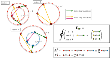
Figure 4: Graphic visualization of the different impurity scattering processes in the 2D Dirac model in different energy $\epsilon$ regimes (I, II and III; see Fig. 1; main text). We report graphically the different relaxation rates $\Lambda_{\chi}^{\pm},\Upsilon_{\chi}^{\pm}$ mentioned in the main text. Colored dots are to be identified with the indices $\chi$. When a generic scattering amplitude (grey segment connecting yellow and green dots) is integrated over the angle, it gives rise to different components of $\boldsymbol{\Gamma}_{\chi\chi^{\prime}}$ depending to which trigonometric function it is contracted with. Combinations of the various components yield the different relaxation rates.

The formal solution of the linear system Eq. (63) gives

$$\boldsymbol{\tau}^{\parallel} =-2\left(\hat{\Lambda}+\hat{\Upsilon}\hat{\Lambda}^{-1}\hat{\Upsilon}\right)^{-1}\boldsymbol{1}\,,$$ (66)

$$\boldsymbol{\tau}^{\perp} =\hat{\Lambda}^{-1}\hat{\Upsilon}\boldsymbol{\tau}^{\parallel}\,,$$ (67)

as reported in Eq. (6) of the main text.

I.1.2 Finite magnetic field

In the presence of an external magnetic field, the LHS of the BTEs reads as

$$\dot{\mathbf{k}}\cdot\nabla_{\mathbf{k}}f_{\mathbf{k}_{\chi}}=-\left(\boldsymbol{\mathcal{E}}+\text{{v}}_{\mathbf{k}}\times\boldsymbol{\mathcal{B}}\right)\cdot\nabla_{\mathbf{k}}\left(f_{\mathbf{k}_{\chi}}^{0}+\delta f_{\mathbf{k}_{\chi}}\right)\,.$$ (68)

In the linear response regime, the contraction with the electric field only selects the equilibrium part $f_{\mathbf{k}_{\chi}}^{0}$, as seen above. On the other hand, the contraction with the magnetic field selects the non-equilibrium part since

$$\left(\text{{v}}_{k}\times\boldsymbol{\mathcal{B}}\right)\cdot\text{{v}}_{k}=0\,.$$ (69)

It is thus convenient to use the following generalized ansatz:

$$\delta f_{\mathbf{k}_{\chi}}=v_{\mathbf{k}_{\chi}}\left(\tau_{\chi}^{\parallel}\cos\phi_{\mathbf{k}}+\tau_{\chi}^{\perp}\sin\phi_{\mathbf{k}}\right)\,.$$ (70)

In evaluating the term $\nabla_{\mathbf{k}}\delta f_{\mathbf{k}_{\chi}}$, we use the relations between cartesian and polar derivates

$$\frac{\partial}{\partial k_{x}}=\cos\phi_{\mathbf{k}}\frac{\partial}{\partial k}-\frac{\sin\phi_{\mathbf{k}}}{k}\frac{\partial}{\partial\phi_{\mathbf{k}}}\,,$$ (71)

$$\frac{\partial}{\partial k_{y}}=\sin\phi_{\mathbf{k}}\frac{\partial}{\partial k}+\frac{\cos\phi_{\mathbf{k}}}{k}\frac{\partial}{\partial\phi_{\mathbf{k}}}\,.$$ (72)

We thus have (omitting the index $\chi$ in the intermediate steps)

$$\left(\text{{v}}_{\mathbf{k}}\times\boldsymbol{\mathcal{B}}\right)\cdot\nabla_{\mathbf{k}}\delta f_{\mathbf{k}} =\epsilon_{abc}v_{\mathbf{k}}^{a}\mathcal{B}_{b}\,\partial_{c}\left[v_{\mathbf{k}}\left(\tau^{\parallel}\cos\phi_{\mathbf{k}}+\tau^{\perp}\sin\phi_{\mathbf{k}}\right)\right]\,,$$ (73)

where $\epsilon_{abc}$ is the Levi-Civita symbol. Expanding the derivatives (and using $\partial_{k_{i}}\to\partial_{i}$ for brevity), we obtain

$$1.\quad\>\partial_{x}\left[v_{\mathbf{k}}\left(\tau^{\parallel}\cos\phi_{\mathbf{k}}+\tau_{\chi}^{\perp}\sin\phi_{\mathbf{k}}\right)\right] =\cos^{2}\phi_{\mathbf{k}}\,\partial_{k}\left(v_{\mathbf{k}}\tau^{\parallel}\right)+\cos\phi_{\mathbf{k}}\sin\phi_{\mathbf{k}}\partial_{k}\left(v_{\mathbf{k}}\tau^{\perp}\right)+$$

$$+\tau^{\parallel}\,v_{\mathbf{k}}\,\partial_{x}\cos\phi_{\mathbf{k}}+\tau^{\perp}v_{\mathbf{k}}\,\partial_{x}\sin\phi_{\mathbf{k}\,,}$$ (74)

$$2.\quad\>\partial_{y}\left[v_{\mathbf{k}}\left(\tau^{\parallel}\cos\phi_{\mathbf{k}}+\tau_{\chi}^{\perp}\sin\phi_{\mathbf{k}}\right)\right] =\sin\phi_{\mathbf{k}}\cos\phi_{\mathbf{k}}\,\partial_{k}\left(v_{\mathbf{k}}\tau^{\parallel}\right)+\sin^{2}\phi_{\mathbf{k}}\,\partial_{y}\left(v_{\mathbf{k}}\tau^{\perp}\right)+$$

$$+\tau^{\parallel}v_{\mathbf{k}}\,\partial_{y}\cos\phi_{\mathbf{k}}+\tau^{\perp}v_{\mathbf{k}}\,\partial_{y}\sin\phi_{\mathbf{k}\,,}$$ (75)

where we assumed an isotropic Fermi surface $\mathbf{k}\parallel\text{{v}}$. These expressions, using Eqs. (71)-(72), can be rewritten as

$$1.\quad \cos^{2}\phi_{\mathbf{k}}\,\partial_{k}\left(v_{\mathbf{k}}\tau^{\parallel}\right)+\cos\phi_{\mathbf{k}}\sin\phi_{\mathbf{k}}\,\partial_{k}\left(v_{\mathbf{k}}\tau^{\perp}\right)+v_{\mathbf{k}}\frac{\tau^{\parallel}}{k}\sin^{2}\phi_{k}-v_{\mathbf{k}}\frac{\tau^{\perp}}{k}\sin\phi_{\mathbf{k}}\cos\phi_{\mathbf{k}}\,,$$ (76)

$$2.\quad \sin\phi_{\mathbf{k}}\cos\phi_{\mathbf{k}}\,\partial_{k}\left(v_{\mathbf{k}}\tau^{\parallel}\right)+\sin^{2}\phi_{\mathbf{k}}\,\partial_{k}\left(v_{\mathbf{k}}\tau^{\perp}\right)-v_{\mathbf{k}}\frac{\tau^{\parallel}}{k}\sin\phi_{\mathbf{k}}\cos\phi_{\mathbf{k}}+v_{\mathbf{k}}\frac{\tau^{\perp}}{k}\cos^{2}\phi_{\mathbf{k}}\,.$$ (77)

Taking a perpendicular magnetic field $\boldsymbol{\mathcal{B}=}\mathcal{B}\,\hat{z}$, one obtains after standard algebraic manipulations

$$\left(\text{{v}}_{\mathbf{k}_{\chi}}\times\boldsymbol{\mathcal{B}}\right)\cdot\nabla_{\mathbf{k}}\delta f_{\mathbf{k}_{\chi}} =v_{\mathbf{k}_{\chi}}\omega_{\mathcal{B}}^{\chi}\left(\tau_{\chi}^{\parallel}\sin\phi_{\mathbf{k}_{\chi}-}\tau_{\chi}^{\perp}\cos\phi_{\mathbf{k}_{\chi}}\right)\,,$$ (78)

where we reinstated the index $\chi$ and defined the cyclotronic frequency of the $\chi$-ring

$$\omega_{\mathcal{B}}^{\chi}=\frac{v_{\mathbf{k}_{\chi}}}{k_{\chi}}\mathcal{B}\,.$$ (79)

It is clear from Eq. (35)-(36), that $\omega_{\mathcal{B}}^{\chi}$ can be reabsorbed in the definition of the skew cross sections:

$$\Gamma_{\chi\chi}^{\text{sin}}\to\Gamma_{\chi\chi}^{\text{sin}}+\omega_{B}^{\chi}\,,$$ (80)

to which the trivial generalization of Eqs. (63) follows. Note however, due to the slight different ansatz we have used, the column of the know terms $-2\textrm{$\left(\boldsymbol{1},\boldsymbol{0}\right)$}^{\textrm{t}}$ has to be generalized to $-2F_{\chi}\left(\boldsymbol{1},\boldsymbol{0}\right)^{\textrm{t}}$.

I.2 TRANSVERSE SCATTERING CROSS SECTION: ELASTIC AND SPIN-FLIP CHANNELS

Below, we discuss the effective “spin-Lorentz forces” responsible for the sign-change in the extrinsic transverse response and show that the outer ring $\chi=1$ generally yields the dominant contribution to the Hall conductivity in the weak scattering limit.

I.2.1 Scattering in region I and II: intra-ring transition and main contribution from $\chi=1$ ring

The starting point is the expression for the single-valley Hall conductivity at $T=0$,

$$\sigma_{\perp}=\frac{e^{2}}{h}\sum_{\chi=\pm 1}k_{\chi}v_{\chi}\tau_{\chi}^{\perp}\,.$$ (81)

Clearly, the peculiar sign-change must result from the energy dependence of transverse scattering times $\tau_{\chi}^{\perp}$. In Fig. (5) we show a comparison between the two $\tau_{\chi}^{\perp}$ where inter-ring transition are neglected. Both $\tau_{\chi}^{\perp}$ change sign, although $|\tau_{+}^{\perp}|>|\tau_{-}^{\perp}|$. The outer ring is also associated with a larger density of states $N_{+}>N_{-}$ , where $N_{\chi}=k_{\chi}|2\pi v_{k_{\chi}}|^{-1}$, as displayed in Fig. 5(b). The larger $\tau_{+}^{\perp}$ and $N_{+}^{\perp}$ as compared to their $\chi=-1$ counterparts motivate our discussion in the main text concerning the change of sign of $\sigma_{\perp}$ focused on $\text{{k}}_{+}\to\text{{k}}_{+}$ transitions. In addition, the out-of-plane spin polarization $S^{z}$ also changes sign within the $\chi=1$ ring, as displayed in Fig. 5(c) and (d).

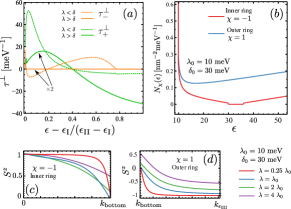
Figure 5: (a) Transverse scattering time in two cases of interest $\lambda\gtrless\delta$, where the larger and smaller energy scales are, respectively, 10 and 30 meV. The change of sign is clearer for $\tau_{+}^{\perp}$. (b) Also the density of states of the outer ring is generally larger (here $\lambda>\delta$). (c) Finally it is shown the sign change in the out-of-plane spin polarization happens within the ring $\chi=1$. Parameters: $u_{0}=0.36$ eV$\cdot$nm^-2 and $n_{i}=10^{12}\,\text{cm}^{-2}$.

I.2.2 Spin-conserving and spin-flip Lorentz force from the collision integral

Having demonstrated the dominant role played by intra-ring $\chi$=1 processes, we now discuss the physical picture behind the sign-change in $\sigma_{\perp}$ as the Fermi level approaches the spin majority band edge. The transverse relaxation time, in the absence of a magnetic field, is given by

$$\tau_{+}^{\perp}=\frac{\Gamma_{++}^{\text{sin}}}{(\Gamma_{++}^{\text{0}}-\Gamma_{++}^{\cos})^{2}+(\Gamma_{++}^{\text{sin}})^{2}}\,,$$ (82)

and hence the change of sign of $\tau_{+}^{\perp}$ is controlled by the antisymmetric part of $\mathcal{T}_{++}(\phi)=|\langle\mathbf{k_{+}^{\prime}|}t|\mathbf{k}_{+}\rangle|^{2}.$ The single-impurity $T$ matrix can be decomposed according to the following form

$$t=t_{0}\gamma_{0}+t_{\text{KM}}\gamma_{\text{KM}}+t_{z}\,s_{z}+t_{m}\Sigma_{z}+t_{r}\gamma_{r}\,.$$ (83)

Importantly, all terms are associated with diagonal matrices in spin space, except the “Rashba term” $T_{r}\gamma_{r}$. The latter is indeed what connects orthogonal spin states. The resulting terms in $\Gamma_{++}^{\sin}$ lead to the effective spin-conserving and spin-flip Lorentz forces, as described in the main text. In Fig. 6 we plot the modulus square of $\mathcal{T}_{++}(\phi)$ as a function of the scattering angle and for different values of the Fermi energy $\epsilon$ lying in region I or II.

Figure 6: Effective spin-conserving and the spin-flip Lorentz forces. Parameters: $u_{0}=0.036$ eV$\cdot$nm^-2 and $n_{i}=10^{12}\,\text{cm}^{-2}$.

I.3 ADDITIONAL DISCUSSIONS

I.3.1 Thermal fluctuations

The finite temperature transverse response is obtained from

$$\sigma_{\perp}^{T}(\mu)=-\int_{-\infty}^{+\infty}d\epsilon\,\left(\frac{\partial f^{0}(\epsilon,\mu,T)}{\partial\epsilon}\right)\sigma_{\perp}^{T=0}(\epsilon)\,,$$ (84)

where $\sigma_{\perp}^{T=0}(\epsilon)$ is the zero-temperature response and $f^{0}(\epsilon,\mu,T)=\left(1+\text{Exp}\left[\left(\epsilon-\mu\right)/k_{B}T\right]\right)^{-1}$. Figure  (7) shows the temperature dependence of the anomalous Hall conductivity for typical parameters. The characteristic change of sign is visible up to temperatures $T\approx T_{\text{room}}/2$.

I.3.2 Intervalley scattering

To account for intervalley scattering, we use the following simplified model for the disorder potential with site $C_{6v}$ symmetry:

$$V\left(\text{{x}}\right)=\sum_{i=1}^{N_{i}}\,R^{2}(u_{0}\gamma_{0}+u_{x}\tau_{x})\delta(\text{{x}}-\boldsymbol{\text{{x}}}_{i})\,,$$ (85)

which interpolates between a pure intravalley potential $(u_{x}=0)$ and a atomically-sharp potential with $u_{x}=u_{0}$ (e.g., a resonant adatom) leading to strong intervalley scattering Impurities_G_Basko ; supp2_Pachoud . The intervalley term ($u_{x}$) introduces new rates:

$$\boldsymbol{\Gamma}_{\chi\zeta}=\left\{\Gamma_{\chi\zeta}^{0},\Gamma_{\chi\zeta}^{\cos},\Gamma_{\chi\zeta}^{\text{sin}}\right\}=2\pi n_{i}\int(d^{2}\text{{k}}^{\prime})\,\left\{1,\cos\phi,\sin\phi\right\}\mathcal{T}_{\chi\zeta}(\phi)\,,$$ (86)

where $\zeta=\pm 1$ is an index associated with outer and inner ring respectively for states at $K^{\prime}$ valley, obtainable from Eq. (3) of the main text by performing the substitution $\lambda,v\to-\lambda,-v$. We plot the result in Fig. 7. The intervalley scattering results in a reduction of the total transverse relaxation time.

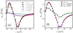
Figure 7: Effect of thermal fluctuations and intervalley scattering. (a) Change of sign in $\sigma_{\perp}$ is distinguishable for $T\lesssim T_{\text{room}}/2$, where $T_{\text{room}}=300\,\text{K}$. (b) In the less favorable scenario ($u_{x}=u_{0}$), the transport times $\tau^{\parallel,\perp}(\epsilon)$ are reduced by a factor $\approx 2$. Parameters: $u_{0}=3.6$ eV$\cdot$nm^-2 and $n=10^{12}\,\text{cm}^{-2}$.

I.3.3 Magnetic field

The formalism at finite magnetic field [Sec. (I.1.2)] allows us to model various quantities of interest in graphene/thin film heterostructures. Figure 8 shows the anomalous Hall resistivity $\rho_{\text{AH}}$ as function of the applied magnetic field. To reproduce a typical hysteresis loop for magnetized graphene, the effective exchange coupling is chosen as $\delta_{\text{eff}}=\delta\,\text{tanh}\left(\mathcal{B}/\mathcal{B}_{\text{sat}}\right)$, where $\delta=30$ meV, and with the saturation field $\mathcal{B}_{\text{sat}}=1.5\times 10{}^{3}\text{Gauss}$ Ferr_G_YIG_Wang15 ; AHE_G_Tang_18 .

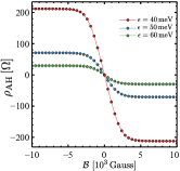
Figure 8: $\rho_{\text{AH}}$ as a function of the magnetic field for different Fermi energies $\epsilon$. Parameters: $\lambda=10\,\text{meV},$ $u_{0}=1$ eV$\cdot$nm^-2 and $n_{i}=10^{12}$. Also $\delta_{\text{eff}}=\delta\,\text{tanh}\left(\mathcal{B}/\mathcal{B}_{\text{sat}}\right)$, $\delta=30$ meV, and $\mathcal{B}_{\text{sat}}=1.5\times 10{}^{3}\text{Gauss}$ AHE_G_Tang_18 .

II EQUIVALENCE BETWEEN SEMICLASSICAL AND KUBO-STREDA FORMALISM

We evaluate the disorder correction to the anomalous Hall conductivity by means of linear response theory supp_2bStreda ; supp3_Crepieux ; supp4_Sinitsyn ; Ado2015 ; milletari16 . The results are shown to agree with the BTEs to numerical accuracy.

II.1 Linear response formalism

The longitudinal (Drude) and transverse (Hall) responses are denotes as $\sigma_{xx}$ and $\sigma_{yx}$, respectively. The transverse response is calculated using the Kubo-Streda formalism supp_2bStreda , $\sigma_{yx}(\epsilon)=\sigma_{yx}^{I}(\epsilon)+\sigma_{yx}^{II}(\epsilon)\,,$ where Comment2

$$\sigma_{yx}^{I}(\epsilon) =\int(d\mathbf{k})\,\text{tr}\left(v_{y}\mathcal{G}_{\mathbf{k}}^{R}(\epsilon)\tilde{v}_{x}(\epsilon)\mathcal{G}_{\mathbf{k}}^{A}(\epsilon)\right)\,,$$ (87)

$$\sigma_{yx}^{II}(\epsilon) =-\int_{-\infty}^{\epsilon}d\omega\int(d\mathbf{k})\,\text{Re}\left(\text{tr}\left(v_{x}\frac{d\mathcal{G}_{\mathbf{k}}^{R}(\epsilon)}{d\epsilon}v_{y}\mathcal{G}_{\mathbf{k}}^{R}(\epsilon)-v_{x}\mathcal{G}_{\mathbf{k}}^{R}(\epsilon)v_{y}\frac{d\mathcal{G}_{\mathbf{k}}^{R}(\epsilon)}{d\epsilon}\right)\right)\,,$$ (88)

and

$$\mathcal{G}_{\mathbf{k}}^{R/A}(\epsilon)=\left(\epsilon-H_{0\mathbf{k}}-\Sigma^{R/A}\right)^{-1}\,,$$ (89)

are disorder averaged Green’s functions associated with the Hamiltonian Eq. (1) of the main text and $\Sigma^{R/A}=n_{i}t^{R/A}$ is the self energy. Here, tr is the trace over internal degrees of freedom $\tau,\Sigma,s$ and $v_{x,y}=\partial_{k_{x,y}}H_{0\boldsymbol{k}}=\tau_{z}\sigma_{x,y}$ are the bare current operators. $\tilde{v}_{x}$ is the renormalized current vertex, obtained from the Bethe-Salpeter (BS) equation

$$\tilde{v}_{x}(\epsilon)=v_{x}+n_{i}\,\text{tr}\,\sum_{\mathbf{k}}t^{R}(\epsilon)\,\mathcal{G}_{\mathbf{k}}^{R}(\epsilon)\,\tilde{v}_{x}(\epsilon)\,t^{A}(\epsilon)\,\mathcal{G}_{\mathbf{k}}^{A}(\epsilon)\,.$$ (90)

$\sigma_{yx}^{I},\sigma_{yx}^{II}$ are the so-called “Fermi surface” and “Fermi sea” contribution to the Hall response . The semiclassical (skew scattering) contribution originates from the leading disorder correction, $\sigma_{\perp}\propto\tau^{\perp}\propto n_{i}^{-1}$ milletari16 .

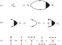
Figure 9: $T$-matrix ladder resummation for the renormalized charge vertex entering the transverse response milletari16 . (a) the solid line with arrow towards right (left) represents a renormalized propagator projected on the retarded (advanced) sector. (b) diagrammatic representation of the Bethe-Salpeter $T$-matrix ladder, as shown in (c). Black (white) boxes correspond to $T^{R}$($T^{A}$), red crosses to impurity density insertions and black dot to single impurity scattering potential $u_{0}$.

II.1.1 Disorder averaged Green’s function

We provide the explicit form of the disorder averaged Green’s function for intravalley scattering potentials ($u_{x}=0$). To obtain those, one first needs to calculate the disorder averaged $T$ matrix

$$t^{R/A}=\langle V(1-g_{0}^{R/A}V)^{-1}\rangle_{\text{dis}}\,,$$ (91)

where the momentum-integrated bare Green’s function reads as

$$g_{0}^{R,A} =-\frac{1}{2}\left\{\left(\epsilon\,\gamma_{0}-\delta\,s_{z}\right)L_{+}^{R,A}+\frac{1}{D}\left[\epsilon\left(\lambda^{2}+\delta^{2}\right)\gamma_{0}-\delta\left(\epsilon^{2}-\lambda^{2}\right)\,s_{z}+\delta\,\lambda^{2}\,\gamma_{m}+\epsilon\,\lambda^{2}\gamma_{\text{KM}}-\lambda\left(\epsilon^{2}-\delta^{2}\right)\gamma_{r}\right]L_{-}^{R,A}\right\}\,,$$ (92)

with $D=\sqrt{\epsilon^{2}\delta^{2}+\lambda^{2}\left(\epsilon^{2}-\delta^{2}\right)}$ . Also we have defined $L_{\pm}^{p}=L_{1}^{p}\pm L_{2}^{p}$ ($p=R/A=\pm$) with

$$L_{1,2}^{p} =\frac{1}{v^{2}k^{2}-z_{1,2}^{p}}\,,\;\;\;z_{1,2}^{p}=\epsilon^{2}+\delta^{2}\pm 2\,D+i\,p\,0^{+}\,.$$ (94)

Beyond the identity and the matrix structures $\gamma_{r},s_{z}$, already present in the bare Hamiltonian, we obtain two additional terms $\gamma_{m}=\Sigma_{z},\,\gamma_{\text{KM}}=\Sigma_{z}s_{z}$, which will appear in the self-energy and thus in the disorder averaged Green’s functions.

To obtain an analytical expression for $\mathcal{G}_{\mathbf{k}}^{R/A}(\epsilon)$, we consider an effective model containing all the matrix structures appearing in $g_{0}^{R/A}$, namely

$$H_{\text{eff}}=H_{0}+m\,\gamma_{\text{KM}}+\lambda_{m}\gamma_{m}\,.$$ (95)

The disorder averaged Green’s function of the original Hamiltonian Eq. (1) in the main text for $u_{x}=0$ is obtained by taking the bare Green’s function of Eq. (95) and performing the following analytical continuations

$$\mathcal{A}^{R/A}:\>\epsilon \to \epsilon-n_{i}(\epsilon\pm i\eta_{0})\,,$$ (96)

$$\lambda \to \lambda+n_{i}\left(\varDelta\lambda\pm i\eta_{r}\right)\,,$$

$$\delta \to \delta+n_{i}\left(\varDelta\delta\pm i\eta_{z}\right)\,,$$ (97)

$$m_{0} \to n_{i}(\varDelta m\pm i\eta_{\text{KM}})\,,$$

$$\lambda_{m} \to n_{i}\left(\varDelta\lambda_{m}\pm i\eta_{m}\right),$$ (98)

where the parameters defined by

$$\varDelta\lambda_{i}+i\eta_{i}=\frac{1}{8}\text{tr}[t^{R}\gamma_{i}]\,,$$ (99)

and $\lambda_{i},\eta_{i}$ denote, respectively, the real and imaginary parts of one of the parts of the $T$ matrix associated with the matrix $\gamma_{i}$. We then find

$$\mathcal{G}^{p} =\left.\sum_{\xi=\pm}\left(\mathcal{M}_{0,\xi}+\mathcal{M}_{\phi_{\text{{k}}},\xi}\right)\mathcal{L}_{\xi}\right|_{\mathcal{A}^{p}}\,,$$ (100)

meaning that the analytical continuation $\mathcal{A}^{p}$ has to be performed to find the $p=R/A$ sectors. Above, expressing the matrices in the notation $\mathcal{M}=\tau_{i}\otimes\mathcal{\tilde{M}}\,,\mathcal{\tilde{M}}_{jk}=1/4\,\text{tr}\left[\mathcal{\tilde{\mathcal{M}}}\sigma_{j}s_{k}\right]$, we have explicitly

$$\mathcal{M}_{0,+}= -\frac{\tau_{0}}{2}\left(\begin{array}[]{cccc}\epsilon&0&0&-\delta\\ 0&0&0&0\\ 0&0&0&0\\ \lambda_{m}&0&0&m\end{array}\right)\,,$$ (105)

$$\mathcal{M}_{0,-}= -\frac{\tau_{0}}{2\tilde{\Gamma}}\left(\begin{array}[]{cccc}\left[\epsilon\left(\lambda^{2}+\delta^{2}\right)+m\left(\lambda_{m}\,\delta-\lambda^{2}\right)\right]&0&0&\left[\delta^{2}\left(\lambda_{m}+\delta\right)-\epsilon\left(m\,\lambda_{m}+\epsilon\,\delta\right)\right]\\ 0&0&0&0\\ 0&0&0&0\\ \left[\lambda^{2}\left(\lambda_{m}+\delta\right)-m\left(\epsilon\,\delta+m\,\lambda_{m}\right)\right]&0&0&\left[\epsilon\left(\lambda^{2}-\delta\,\lambda_{m}\right)-m\left(\lambda^{2}+\lambda_{m}^{2}\right)\right]\end{array}\right)$$ (110)

$$-\frac{\delta}{2\tilde{\Gamma}}\left[\left(\lambda_{m}+\delta\right)^{2}-\left(\epsilon-m\right)^{2}\right]\gamma_{r}\,,$$ (111)

and

$$\mathcal{M}_{\phi_{\text{{k}}},+} =-\frac{\tau_{z}}{2}\left(\begin{array}[]{cccc}0&0&0&0\\ vk\,\cos\phi_{\text{{k}}}&\lambda\sin 2\phi_{\text{{k}}}&-\lambda\cos 2\phi_{\text{{k}}}&0\\ vk\,\sin\phi_{\text{{k}}}&-\lambda\cos 2\phi_{\text{{k}}}&-\lambda\sin 2\phi_{\text{{k}}}&0\\ 0&0&0&0\end{array}\right)$$ (116)

$$\mathcal{M}_{\phi_{\text{{k}}},-} =-\frac{\tau_{0}}{2\tilde{\Gamma}}\left(\begin{array}[]{cccc}0&vk\left(\epsilon-m\right)\lambda\,\sin\phi_{\text{{k}}}&-vk\left(\epsilon-m\right)\lambda\,\cos\phi_{\text{{k}}}&0\\ 0&0&0&0\\ 0&0&0&0\\ 0&vk\,\lambda\left(\lambda_{m}+\delta\right)\sin\phi_{\text{{k}}}&-vk\,\lambda\left(\lambda_{m}+\delta\right)\cos\phi_{\text{{k}}}&0\end{array}\right)$$ (121)

$$-\frac{\tau_{z}}{4\tilde{\Gamma}}\left(\begin{array}[]{cccc}0&0&0&0\\ 0&\lambda\left(\epsilon^{2}+\delta^{2}-m^{2}-\lambda_{m}\right)\,\sin 2\phi_{\text{{k}}}&-\lambda\left(\epsilon^{2}+\delta^{2}-m^{2}-\lambda_{m}\right)\,\cos 2\phi_{\text{{k}}}&-vk\,(m\lambda_{m}+\epsilon\delta)\cos\phi_{\text{{k}}}\\ 0&-\lambda\left(\epsilon^{2}+\delta^{2}-m^{2}-\lambda_{m}\right)\,\cos 2\phi_{\text{{k}}}&-\lambda\left(\epsilon^{2}+\delta^{2}-m^{2}-\lambda_{m}\right)\,\sin 2\phi_{\text{{k}}}&-vk\,(m\lambda_{m}+\epsilon\delta)\sin\phi_{\text{{k}}}\\ 0&0&0&0\end{array}\right)$$ (126)

with

$$\tilde{\Gamma} =\sqrt{\delta^{2}\left[\left(m-\epsilon\right)^{2}-\left(\lambda_{m}+\delta\right)^{2}\right]+\left(m\,\lambda_{m}+\epsilon\,\delta\right)^{2}}$$ (127)

$$\mathcal{L}_{\pm} =\left[v^{2}k^{2}-\left(\epsilon^{2}+\delta^{2}-m^{2}-\lambda_{m}^{2}\pm 2\tilde{\Gamma}\right)\right]^{-1}\,.$$ (128)

II.1.2 Renormalized charge current vertex: solution of the BS equation and symmetry arguments

Figure 10: Comparison between Kubo–Streda (diagrammatic) and Boltzmann calculation for both the longitudinal and transverse response in a representative case: $u_{0}=0.36$ eV$\cdot$nm^-2 a d $n_{i}=10^{12}\text{cm}^{-2}$. The agreement between the two formalisms is excellent.

The recursive BS equation Eq. (90) for the charge vertex produces new matrix structures, which are associated to observables that can be “excited” upon the application of external fields. We show now how these observables can be predicted by simple symmetry arguments. The continuum model Eq. (1) of the main text is invariant under the following symmetry operations

$$C_{2} : \tau_{x}s_{z}e^{i\pi l_{z}}$$ (129)

$$\Lambda_{z} : \tau_{z}$$ (130)

$$\Lambda_{x} : \tau_{x}\Sigma_{z}$$ (131)

$$\Lambda_{y} : \tau_{y}\Sigma_{z\,.}$$ (132)

$C_{2}$ is the rotation of $\pi$ around the $\hat{z}$-axis, and $l_{z}=-i\partial_{\phi}$ the generator of the rotation in coordinate space. Reflection around $\hat{x}$: $R_{x}:\,\Sigma_{x}s_{y}r_{x}$, with $r_{x}:\;\;(\mathbf{x},\mathbf{y})\to(\mathbf{x},-\mathbf{y})\,,$ and time reversal operation $\Theta$, present in the continuum limit of bare graphene, are broken symmetries in this model; we can refer to the transformations above as pseudosymmetries

$$\text{$\Theta$}^{-1}\,H\left(\delta\right)\,\Theta =H\left(-\delta\right)$$ (133)

$$R_{x}^{-1}\,H\left(\delta\right)\,R_{x} =H\left(-\delta\right)\,.$$ (134)

To constraint the number of observables with nonzero expectation value, we examine the generic response function

$$\mathcal{R}_{\alpha}=\text{Tr$\left[\gamma_{\alpha}\,G_{0}^{R}v_{x}\,G_{0}^{A}\right]$\,,}$$ (135)

for an observable $\gamma_{\alpha}$. In the above, Tr includes the trace in momentum space. Exploring any of the symmetries $\mathcal{S}$ listed in Eqs. (129)-(132)

$$\mathcal{S}:\,\,G_{0}^{R,A}\to G_{0}^{R,A}\,.$$ (136)

Eq. (135) can be manipulated as follows

$$\mathcal{R}_{\alpha} =\text{Tr}\left[\left(\mathcal{S}\gamma_{\alpha}\mathcal{S}^{\dagger}\right)\left(\mathcal{S}\,G_{0}^{R}\mathcal{S}^{\dagger}\right)\left(\mathcal{S}v_{x}\mathcal{S}^{\dagger}\right)\left(\mathcal{S}\,G_{0}^{A}\mathcal{S}^{\dagger}\right)\right]$$ (137)

$$=\epsilon_{x}\epsilon_{\alpha}\text{Tr}\left[\gamma_{\alpha}\,G^{R}v_{x}\,G^{A}\right]\,,$$ (138)

where $\epsilon=\pm 1$ is the parity of some operator under $\mathcal{S}$. From the last equation, we see that a non-zero response requires the operator $\gamma_{\alpha}$ to have the same parity of the current vertex $v_{x}$ under the action of $\mathcal{S}$. We have

$$C_{2} : v_{x}\to-v_{x}\,,$$ (139)

$$\Lambda_{x,y,z} : v_{x}\to+v_{x}\,.$$ (140)

By spanning the 64-dimensional algebra $\tau_{i}\sigma_{j}s_{k}$, we conclude that only eight responses are allowed

$$\tau_{0}\Sigma_{0}s_{x,y} :$$ spin-x,y (spin-Galvanic) magnetisation (141)

$$\tau_{0}\Sigma_{z}s_{x,y} :$$ staggered spin-x,y polarization (142)

$$\tau_{z}\Sigma_{x,}s_{0,z} :$$ x-charge current (Drude) and spin-z x-current (143)

$$\tau_{z}\Sigma_{y}s_{0,z} : \text{charge y-current (Hall) and z-spin y-current (spin Hall)}\,.$$ (144)

We verified this is confirmed by explicit diagrammatic calculation. Solution of Eq. (90) then requires the inversion of a $8\times 8$ matrix. The solution can be written in the form

$$\tilde{v}_{x}=\sum_{i}v_{x}^{i}\gamma_{i}\,,$$ (145)

where $\gamma_{i}$ as given above. By inserting the renormalized vertex in Eq. (145) into Eq. (87), one can finally find the skew-scattering contribution to the Hall response. One can also calculate the Drude response (xx) by replacing $v_{y}\to v_{x}$ in Eq. (87). Figure 10 benchmarks the BTEs against the diagrammatic formalism.

III SIDE-JUMP CONTRIBUTION

We now evaluate the quantum side-jump (anomalous) contribution to the transverse transport coefficients and show it provides a small correction to the transverse response in clean samples with $k_{F}l\gg 1$. For brevity, we focus here on the AH response. The side-jump contribution $\mathcal{Q}_{yx}$ is obtained by isolating the impurity concentration-independent term

$$\sigma_{yx}^{I}=\frac{\mathcal{S}_{yx}}{n_{i}}+\mathcal{Q}_{yx}+O(n_{i})\,.$$ (146)

Within the rigorous diagrammatic formalism, this requires the calculation of the ladder series for the renormalized vertex (see Fig. 9). In Fig.  11 we plot the ratio $\mathcal{S}_{yx}/n_{i}\mathcal{Q}_{yx}$ at selected SOC values in a system with high mobility. The results show that the side-jump contribution is only sizable in a very narrow energy window, i.e. ~1-10% of the distance between the Rashba edge $\epsilon_{\text{III}}$ and the bottom of the skyrmionic band $\epsilon_{\text{I}}$. The side-jump part rapidly decays to zero, in the diffusive regime with $k_{F}l\gg 1$, thus justifying our approximation in the main text $\sigma_{yx}^{I}\simeq\mathcal{S}_{yx}/n_{i}$. We note that the anomalous term $\mathcal{Q}_{yx}$ also receives contribution from the so-called $\Psi$ and $X$ diagrams encoding quantum coherent skew scattering not evaluated here (see milletari16 for more details).

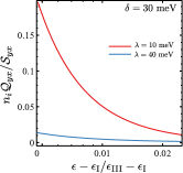
Figure 11: Ratio of the side-jump and skew scattering contribution to $\sigma_{yx}^{I}$ in high mobility samples. The side-jump contribution is negligible away from the Dirac point $k_{F}l\gg 1$. Parameters: $\lambda=$10 meV (red line) and $\lambda=40$ meV (blue line), $\lambda_{z}=30$ meV, $u_{0}=1$ eV$\cdot$nm^-2 and $n_{i}=10^{10}$ cm^-2.

IV INTRINSIC CONTRIBUTION TO THE AHE

In this section we give details about the calculation of the intrinsic contribution to the AHE. This can be done in two equivalent ways: via a direct Berry-curvature calculation or using the clean limit of the Kubo-Streda formula. We show they provide the same result.

IV.0.1 Kubo-Streda approach

We start here by computing the intrinsic contribution within the Kubo-Streda formalism. In practice, one needs to evaluate Eqs. (87)-(88) in the clean limit, which corresponds to the substitution for the Green’s functions $\mathcal{G}_{\mathbf{k}}^{a}\to G_{0\mathbf{k}}^{a}$. Using the expression presented above for the latter, we can extract the (single valley) $\sigma^{I}$ contribution as

$$\sigma_{yx}^{I}\left(\epsilon\right)=-\frac{1}{2}\frac{\lambda^{2}\delta}{\epsilon}\begin{cases}\frac{2\left(3\lambda^{2}\delta^{2}+\delta^{4}-2\epsilon^{2}\left(\lambda^{2}+\delta^{2}\right)\right)}{\left(\lambda^{4}+3\lambda^{2}\delta^{2}+\delta^{4}-\epsilon^{2}\left(\lambda^{2}+\delta^{2}\right)\right)\sqrt{\epsilon^{2}\left(\lambda^{2}+\delta^{2}\right)-\lambda^{2}\delta^{2}}}&\text{region I}\\ \\ \frac{\left(2+\frac{\lambda}{\sqrt{\epsilon^{2}\left(\lambda^{2}+\delta^{2}\right)-\lambda^{2}\delta^{2}}}\right)}{\lambda^{2}+\delta^{2}+\sqrt{\epsilon^{2}\left(\lambda^{2}+\delta^{2}\right)-\lambda^{2}\delta^{2}}}&\text{region II}\\ \\ \frac{2\left(2\lambda^{2}+\delta^{2}\right)}{\lambda^{4}+3\lambda^{2}\delta^{2}+\delta^{4}-\epsilon^{2}\left(\lambda^{2}+\delta^{2}\right)}\,.&\text{region III}\end{cases}$$ (147)

For the Fermi sea term, $\sigma_{yx}^{II}$ we need instead to calculate the derivative of the Green’s functions with respect to the energy variable. By doing that, performing the trace over internal indices and angular integration we arrive at

$$\sigma_{yx}^{II}(\epsilon)=64\,\lambda^{2}\delta\lim_{\eta\to 0}\text{Im}\left[\int_{-\infty}^{\epsilon}d\omega\int_{0}^{\infty}\frac{dk\,k}{2\pi}\frac{v^{2}k^{2}-\omega^{2}}{(v^{2}k^{2}-z_{1}^{R})^{2}(v^{2}k^{2}-z_{2}^{R})^{2}}\right]\,.$$ (148)

Starting form Eq. (148) we want to perform integration over energies $\int_{\omega}$ first. Doing partial fraction decomposition of the integrand

$$g(k,\omega)=\frac{64\,\lambda^{2}\delta\,(v^{2}k^{2}-\omega^{2})}{(v^{2}k^{2}-z_{+})^{2}(v^{2}k^{2}-z_{-})^{2}}\,,$$ (149)

we look for the poles in $\omega$. Obviously we get the eigenvalues

$$\epsilon_{\mu\nu}(k)=\mu\sqrt{v^{2}k^{2}+2\lambda^{2}+\delta^{2}+\nu\,S_{k}}\,,\qquad S_{k}=\sqrt{v^{2}k^{2}\left(\lambda^{2}+\delta^{2}\right)+\lambda^{4}}\,.$$ (150)

displaced by the small imaginary part $i\eta$. Note the following relations hold for the eigenvalues

$$\epsilon_{++} =-\epsilon_{+-}\,,$$ (151)

$$\epsilon_{--} =-\epsilon_{-+}\,.$$ (152)

Let us write the partial fraction decomposition in the form

$$g(k,\omega) =\frac{A\omega+B}{\left(\omega-\epsilon_{-1}+i\eta\right)^{2}}+\frac{C\omega+D}{\left(\omega-\epsilon_{-2}+i\eta\right)^{2}}+\frac{E\omega+F}{\left(\omega+\epsilon_{-2}+i\eta\right)^{2}}+\frac{G\omega+H}{\left(\omega+\epsilon_{-1}+i\eta\right)^{2}}\,,$$ (153)

where we have labeled the eigenvalues according to the prescription for the contracted index $n$ adopted in the main text

$$\epsilon_{-1} =\epsilon_{+-}$$ (154)

$$\epsilon_{-2} =\epsilon_{--}\,,$$ (155)

which are respectively the lower and the upper branches of the spectrum on the hole side (see Fig. 12).

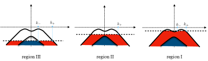
Figure 12: Schematic of band structure in the hole sector and different regimes. Depending on the position of the Fermi level $\epsilon$ the integration over momentum variables has to be performed between different boundaries as reported in details in Table 1.

The eigenvalues appear as poles of second order. As no small $\eta$ is left in the denominator of the $\omega$-independent coefficients $A,B,C,...$, we can focus on the imaginary part of the $\omega$ integration. We basically need to solve two classes of integrals

$$J_{a,b}=\int_{-\infty}^{\epsilon}d\omega\frac{\left(1,\omega\right)}{\left(\omega-\epsilon_{n}+i\eta\right)^{2}}\,.$$ (156)

We have

$$J_{a} =\left.\frac{-1}{\omega-\epsilon_{n}+i\eta}\right|_{-\infty}^{\epsilon}=\frac{-1}{\epsilon-\epsilon_{n}+i\eta}=-\frac{P}{\epsilon-\epsilon_{n}}+i\pi\delta\left(\epsilon-\epsilon_{n}\right)\,,$$ (157)

$$J_{b} =\int_{-\Lambda}^{\epsilon}d\omega\frac{\omega-\epsilon_{n}+i\eta}{\left(\omega-\epsilon_{n}+i\eta\right)^{2}}+\epsilon_{n}\,J_{a}=\log\left|\frac{\epsilon-\epsilon_{n}}{\Lambda}\right|-i\pi\theta\left(\epsilon-\epsilon_{n}\right)+\epsilon_{n}\,J_{a}\,,$$ (158)

where in the last integral we have considered a regularization UV cutoff $\Lambda$. When taking the imaginary part we have

$$J_{a} =i\pi\sum_{\chi=\pm 1}\frac{\delta\left(k-k_{\chi}\right)}{v_{\chi}}\,,$$ (159)

$$J_{b} =-i\pi\left(\theta\left(\epsilon-\epsilon_{n}\right)-\epsilon\sum_{\chi=\pm 1}\frac{\delta\left(k-k_{\chi}\right)}{v_{\chi}}\right)\,,$$ (160)

where we have used $v_{k_{\chi}}\equiv v_{\chi}$. The structure of the integrals Eq. (157)-(158) is important and allows to read already at this stage the quantization of the transverse conductivity. To illustrate that, let us take negative energies, where electronic states can populate bands labeled with $-1,-2$. We can see now how the terms proportional to $\theta,\delta$ in Eqs. (157)-(158) will contribute differently depending on the position of $\epsilon$. In particular we have the following table

$\int_{0}^{\infty}dk\,k\,g(k)\,\,$ I II III gap $\theta\left(\epsilon-\epsilon_{-1}\right)$ = $\int_{k_{-}}^{\infty}dk\,k\,g(k)$ $\int_{0}^{\infty}dk\,k\,g(k)$ $\int_{0}^{\infty}dk\,k\,g(k)$ $\int_{0}^{\infty}dk\,k\,g(k)$ $\theta\left(\epsilon-\epsilon_{-2}\right)$ = $\int_{k_{+}}^{\infty}dk\,k\,g(k)$ $\int_{k_{+}}^{\infty}dk\,k\,g(k)$ $\int_{0}^{k_{-}}dk\,k\,g(k)+\int_{k_{+}}^{\infty}dk\,k\,g(k)$ $\int_{0}^{\infty}dk\,k\,g(k)$ $\delta\left(\epsilon-\epsilon_{-1}\right)$ = $k_{-}g(k_{-})/v_{-}$ 0 0 0 $\delta\left(\epsilon-\epsilon_{-2}\right)$ = $k_{+}g(k_{+})$ $k_{+}g(k_{+})$ $k_{-}g(k_{-})+k_{-}g(k_{-})$ 0

Table 1: Table summarizing the momentum integrals in the different regimes.

The relevant observation is that inside the gap the $\delta$-parts do not contribute, as $\epsilon$ does not intersect any band. Only $\theta$-parts are left, with the integration extending from $0$ to $\infty$. According to the partial fraction decomposition of Eq. (153), we see, by using Eqs. (148), (158), we are left with need to calculate

$$\sigma_{yx}^{II}(\epsilon|_{\text{gap}})=\frac{1}{2\pi}\int_{0}^{\infty}dk\,k\,\left(A+C\right)\,.$$ (161)

In this respect we can identify $A,C\equiv A_{\mathbf{k}},C_{\mathbf{k}}$ as the Berry curvatures of the lower and upper band respectively. We discuss below how they exactly match a direct calculation of the respective Berry curvatures. The analytic expression for the sum $A+C$ is quite complicated. However, explicit calculation shows (re-establishing explicitly the units and considering the contribution of the $K^{\prime}$ valley)

$$\sigma_{yx}^{II}(\epsilon|_{\text{gap}})=\frac{2e^{2}}{h}.$$ (162)

If the Fermi level lies instead outside the gap, $\sigma_{yx}^{II}$ acquires a energy dependence due to non-quantized $\theta$-parts and a finite contribution of the $\delta$-parts. However, we verified the $\delta$-parts cancel exactly opposite in sign contributions in $\sigma_{yx}^{I}(\epsilon)$. A similar cancelation has been reported for a massive Dirac band model in Ref. supp4_Sinitsyn . We conclude the intrinsic contribution is a result of the $\theta$-parts only. Finally note that for positive Fermi we can simply extract the result from what we have obtained in the hole sector; we have in fact $\sigma_{yx}^{\text{int}}(\epsilon)=\sigma_{yx}^{\text{int}}(-\epsilon)$, which is a direct consequence of the Berry curvatures of the bands summing to zero.

IV.0.2 Berry-curvature calculation

We provide details now on a direct calculation of the intrinsic contribution via the Thouless-Kohmoto-Nightingale-Nijs formula TKNNFormula

$$\sigma_{yx}^{\text{int}}(\epsilon)=\sum_{n}\sum_{\mathbf{k}}\Omega_{\mathbf{k}}^{n}\,f^{0}(\epsilon_{n}(k))\,,$$ (163)

where the band-BC is $\Omega_{\mathbf{k}}^{n}=\left(\nabla_{\mathbf{k}}\times\boldsymbol{\mathcal{A}}_{\mathbf{k}}^{n}\right)\cdot\hat{z}$ stemming from the Berry-connection $\boldsymbol{\mathcal{A}}_{\mathbf{k}}^{n}=-i\langle n\mathbf{k}|\nabla_{\mathbf{k}}|n\mathbf{k}\rangle$. Let us focus again on the two bands in the hole sector. Performing the calculation in polar coordinates, we find the Berry-connection only contains the angular components:

$$\left(\boldsymbol{\mathcal{A}}_{\mathbf{k}}^{n=-1}\right)_{\phi} =\frac{\lambda^{2}\delta\left(\delta^{4}+2\lambda^{2}(2v^{2}k^{2}+3S_{k}+3\lambda^{2})+\delta^{2}(3v^{2}k^{2}+3S_{k}+4\lambda^{2})\right)}{\left(S_{k}^{2}\left(v^{2}k^{2}+2S_{k}+\delta^{2}+2\lambda^{2}\right)\right)^{3/2}}\,\,,$$ (164)

$$\left(\boldsymbol{\mathcal{A}}_{\mathbf{k}}^{n=-2}\right)_{\phi} =-\frac{\lambda^{2}\delta\left(\delta^{4}+2\lambda^{2}(2v^{2}k^{2}-3S_{k}+3\lambda^{2})+\delta^{2}(3v^{2}k^{2}-3S_{k}+4\lambda^{2})\right)}{\left(S_{k}^{2}\left(v^{2}k^{2}+2S_{k}+\delta^{2}+2\lambda^{2}\right)\right)^{3/2}}\,,$$ (165)

with $S_{k}=\sqrt{\lambda^{4}+v^{2}k^{2}(\lambda^{2}+\delta^{2})}$. We verified the latter expressions exactly agree respectively with the coefficients $A,C$ of the previous section. It follows the results match those from the Kubo-Streda formalism presented earlier.

References

(1)C. Gong et al. Nature 546,
265 (2017).
(2)B. Huang et al. Nature 546,
270 (2017).
(3)A. G. Swartz , P. M. Odenthal , Y. Hao
, R. S. Ruoff, and R. K. Kawakami, ACS Nano 6, 10063 (2012).
(4) Z. Wang, C. Tang, R. Sachs, Y.
Barlas and J. Shi, Phys. Rev. Lett. 114, 016603 (2015).
(5)C. Tang, B. Cheng, M. Aldosary, Z. Wang, Z.
Jiang, K. Watanabe, T. Taniguchi, M. Bockrath, and J. Shi, APL
Materials 6, 026401 (2018).
(6)J. C. Leutenantsmeyer, A. A.
Kaverzin, M. Wojtaszek, B. J. van Wees. 2D Materials 4, 014001
(2017).
(7)J. Sinova, S. O. Valenzuela, J. Wunderlich,
C. H. Back, and T. Jungwirth. Rev. Mod. Phys. 87,
1213 (2015).
(8)P. Wei et al., Nature Materials
15, 711 (2016).
(9)Y. F. Wu et al., Phys. Rev.
B95, 195426 (2017).
(10)D. Zhong et al., Sci. Adv. 31,
1603113 (2017).
(11)H. Haugen, D. Huertas-Hernando and
A. Braatas, Phys. Rev B 77, 115406 (2008).
(12)Z. Qiao, S. A. Yang, W. Feng,
W.-K. Tse, J. Ding, Y. Yao, J. Wang, and Q. Niu, Phys. Rev.
B 82, 161414(R) (2010).
(13)Q. Sun, Z. Jiang, Y. Yu and X.C. Xie,
Phys. Rev. B 84, 214501 (2011).
(14)H. X. Yang, A. Hallal, D. Terrade,
X. Waintal, S. Roche, and M. Chshiev, Phys. Rev. Lett. 110,
046603 (2013).
(15)D. Marchenko, A. Varykhalov, J.
S.-Barriga, O. Rader, C. Carbone and G. Bihlmayer, Phys. Rev.
B 91, 235431 (2015).
(16)E. I. Rashba, Physical Review B 79,
161409 (2009).
(17)T.-Wei Chen, Z.-R. Xiao, D.-Wei Chiou, and G.-Y.
Guo. Phys. Rev. B 84, 165453 (2011).
(18)Z. Qiao, H. Jiang, X. Li, Y. Yao and Q. Niu,
Phys. Rev. B 85, 115439 (2012). Z. Qiao et al., Phys.
Rev. Lett. 112, 116404 (2014). J. Zhang, B. Zhao, Y. Yao
and Z. Yang, Phys. Rev. B 92, 165418 (2015).
(19)A. Ferreira, T. G. Rappoport, M. A. Cazalilla
and A. H. Castro Neto, Phys. Rev. Lett. 112, 066601 (2014).
(20)D. V. Tuan, J. M. M.-Tejada, X. Waintal,
B. K. Nikolić, S. O. Valenzuela, and
S. Roche, Phys. Rev. Lett. 117, 176602 (2016).
(21)M. Milletarì and A. Ferreira, Phys. Rev. B 94,
134203 (2016); ibidem, 94, 201402(R) (2016).
(22)C. Huang, Y. D. Chong and M. A. Cazalilla,
Phys. Rev. B 94, 085414 (2016).
(23)K. Zollner, M. Gmitra, T. Frank, and J.
Fabian, Phys. Rev. B 94, 155441 (2016).
(24)M. Gmitra, D. Kochan, P. Hogl, and J. Fabian,
Phys. Rev. B 93, 155104 (2016).
(25)Z. Wang, D.-K. Ki, H. Chen, H. Berger,
A. H. MacDonald, and A. F. Morpurgo, Nat. Commun. 6 , 8339
(2015).
(26)J.C. Leutenantsmeyer, A. A. Kaverzin,
M. Wojtaszek and B. J. van Wees. 2D Materials 4, 014001 (2017).
(27)B. F. Miao, S. Y. Huang, D. Qu, and C. L. Chen,
Phys. Rev. Lett. 111, 066602 (2013).
(28)K. S. Das, W. Y. Schoemaker, B. J. van Wees,
and I. J. Vera-Marun, Phys. Rev. B 96, 220408(R) (2017).
(29)S. Iihama, Y. Otani and S. Maekawa, Nature
Electronics 1, 120 (2018).
(30)J. Qi, X. Li, Q. Niu and J. Feng. Phys. Rev.
B 92, 121403(R) (2015).
(31)C. Cheng, J.-T. Sun, X.-R. Chen, H.-X. Fua and
S. Meng, Nanoscale8, 17854 (2016).
(32)Q.-F. Yao, J. Cai, W.-Y. Tong, S.-J. Gong, J.-Q.
Wang, X. Wan, C.-G. Duan, and J. H. Chu, Phys. Rev. B 95,
165401 (2017).
(33)A. Ferreira, J. Viana-Gomes, J. Nilsson,
E. R. Mucciolo, N. M. R. Peres and A. C. Neto, Phys. Rev. B 83,
165402 (2011).
(34)N. M. R. Peres, Rev. Mod. Phys. 82, 2673
(2010).
(35) M. Offidani, M. Milletarì, R. Raimondi and A.
Ferreira, Phys. Rev. Lett. 119, 196801 (2017).
(36)A. Takayama, T. Saro, S. Souma, and T.
Takahashi, Phys. Rev. Lett. 106, 166401 (2011).
(39)A. Pachoud, A. Ferreira, B. Özyilmaz, A. H.
Castro Neto. Phys. Rev. B 90, 035444 (2014).
(40)P. Streda, J. Phys. C: Solid State Phys. 15
, L1299 (1982).
(41)A. Crepieux and P. Bruno, Phys. Rev. B 64,
014416 (2001).
(42)N. A. Sinitsyn, A. H. MacDonald, T. Jungwirth,
V. K. Dugaev, and J. Sinova. Phys. Rev. B 75, 045315(2007).
(43)I. A. Ado, I. A. Dmitriev, P. M. Ostrovsky, and
M. Titov, EPL 111, 37004 (2015).
(44)M. Milletarì and A. Ferreira, Phys. Rev.
B 94, 134203 (2016): 94, 201402 (2016).
(45)In region I, the states
belong to the same Bloch band whereas in region III they
populate the bands. In region II, the only populated state
(ring ) coincides with the Bloch eigenstate
(46)Z. H. Ni, et al. Nano Lett.
10, 3868 (2010).
(47)L. A. Benítez, J. F. Sierra, W. S. Torres, A.
Arrighi, F. Bonell, M. V. Costache, and S. O. Valenzuela, Nature Physics
14, 303 (2018).
(48)A. Cummings, J. H. García, J. Fabian and S.
Roche. Phys. Rev. Lett. 119, 206601 (2017).
(49)T. S. Ghiasi, J. I.-Aynés, A.A. Kaverzin, and
B. J. van Wees. Nano Lett. 17, 7528 (2017).
(50)We assign the label in descending order,
starting from the band of highest energy. Thus,
and .
(51) D. J. Thouless, M. Kohmoto, M. P. Nightingale
and M. den Nijs, Phys. Rev. Lett. 49, 405 (1982); N. Nagaosa,
J. Sinova, S. Onoda, A. H. MacDonald and N. P. Ong, Rev. Mod. Physics
82, 1539 (2010). F. D. M. Haldane, Rev. Mod. Phys. 89,
040502 (2017).
(52)We have exploited the fact that the bands of interest
are isotropic.
(53)D. M. Basko, Phys. Rev. B 78,
115432 (2008).
(54)I. A. Ado, I. A. Dmitriev, P. M. Ostrovsky, and
M. Titov, EPL 111, 37004 (2015).
(55)The superscripts (italic) are not to
be confused with the indices I, II (roman) indicating the
different regimes in the band structure, as depicted in Fig. 1 of
the main text.