Pion nucleus Drell-Yan process and parton transverse momentum in the pion

Abstract

We present a thorough analysis of unpolarized Drell-Yan (DY) pair production in pion-nucleus scattering. On the nucleus side, we use nuclear parton distributions along with parametrisations of the nucleon partonic transverse distribution available in the literature. Partonic longitudinal and transverse distributions of the pion are those obtained in a recent calculation in a Nambu-Jona Lasinio (NJL) framework, with Pauli-Villars regularization. The scale of the NJL model is determined with a minimisation procedure comparing NLO predictions based on NJL evolved pion distributions to rapidity differential DY cross sections data. The resulting distributions are then used to describe, up to next-to-leading logarithmic accuracy, the transverse momentum spectrum of dilepton pairs up to a transverse momentum of 2 GeV. With no additional parameters, fair agreement is found with available pion-nucleus data, confirming the virtues of the NJL description of pion parton structure. We find sizable evolution effects on the shape of the distributions and on the generated average transverse momentum of the dilepton pair. We furthermore discuss the possibility of gaining information about the behavior of the pion unpolarized transverse momentum dependent parton distribution from pion nucleus DY data.

I Introduction

The non perturbative transverse structure of hadrons has attracted recently much attention and the issue of extracting transverse momentum dependendent parton distributions (TMDs) from data taken in different processes in present and forthcoming high-luminosity facilities represents an important goal of nowadays hadronic Physics. In particular, Drell-Yan (DY) pair production Drell:1970wh , discussed in this paper, and semi-inclusive deep inelastic scattering are the main processes under investigation Diehl:2015uka .

The cross section for DY pair production, differential in the transverse momentum of the pair, $q_{T}$, is a particularly suitable observable for this kind of studies. In particular at small $q_{T}$, where the TMD formalism is formulated, fixed order calculation of this process show large logarithmic corrections due to an incomplete cancellation of soft and collinear singularities between real and virtual contributions and need to be resummed to all orders to recover the predictivity of the theory DDT ; PP ; Altarelli:1984pt .

The description of the $q_{T}$ DY spectrum in $pp$ collisions has reached a high degree of sophistication CSS . On one side, theoretical improvements have increased the perturbative accuracy of the predictions Bozzi:2008bb ; Bozzi:2010xn ; Catani:2015vma ; Catani:2000vq ; deFlorian:2000pr . On the other side, global fits of DY production at different energies have given access to the non perturbative proton transverse structure BLNY ; KN05 . Both aspects have received increasing attention due to the formalisation of new and old concepts in the TMD language AR ; Bacchetta:2017gcc ; Scimemi ; Su:2014wpa . While there are differences between the language used in the modern and the older TMD approaches, physical results should not depend on it. A detailed comparison of the formalisms can be found in Refs. Prokudin:2015ysa ; Ceccopieri:2014qha .

At high energy colliders, this improved knowledge aims to an increasingly better description of electroweak bosons production, with the Higgs $q_{T}$ spectrum being the highlighted case. Measurements of $q_{T}$ spectrum of the DY process, at lower centre of mass energies, are instead more sensitive to the hadronic non perturbative transverse structure.

DY pair production in pion-nucleus scattering is a unique probe of pion parton distribution functions (PDFs) and, as such represents a source of information on the pion parton structure. In particular for the $q_{T}$ spectrum this was realized long time ago by the authors of Ref. Chiappetta:1981vv . More recently, phenomenological analyses have appeared Pasquini:2014ppa . A fit to the $q_{T}$ spectrum of DY pairs produced in pion-nucleus collisions has been recently presented in Ref. Wang:2017zym .

Pion TMDs, which could be extracted in principle in a next generation of pion-nucleus DY experiments COMPASSII-proposal , have received recently considerable theoretical interest, Engelhardt:2015xja ; Musch:2011er ; Lu:2004hu ; Gamberg:2009uk ; Lu:2012hh ; Pasquini:2014ppa ; ns ; Bacchetta:2017vzh . In this paper we study the DY unpolarized pair production in pion-nucleus scattering, to next-to-leading logarithmic (NLL) perturbative accuracy, up to a transverse momentum of the produced lepton pair of 2 GeV. As non perturbative inputs, we use, for the bound nucleons, a longitudinal structure which takes into account nuclear effects and, for the transverse structure, a well established parameterization obtained through a phenomenological fit to proton-proton DY data (called, from now on, KN05 prescription) KN05 . For the pion, we use TMDs obtained in a recent calculation ns , within a Nambu-Jona Lasinio (NJL) framework Klevansky:1992qe , with Pauli-Villars regularization. The corresponding RGE scale of the model is determined in a novel way by comparing the DY unpolarized cross section, integrated over $q_{T}$, described by evolved pion PDFs evaluated in the NJL model to the data.

The aim of the present paper is to study the performances of the NJL model, widely used to describe the non-perturbative meson structure, against DY differential cross section data for the first time. We also analyze to what extent this process can be used to obtain information on the pion transverse structure in momentum space, as it happens for the proton in the corresponding process.

The paper is structured as follows. In the next section, we present the set-up of the calculation and introduce the ingredients used to describe the proton and pion structure. In the third section, we discuss the results of the calculation of DY cross sections in the kinematics of presently available data for pion-tungsten scattering. Eventually, we draw our conclusions in the last section.

II Setting-up the calculation

II.1 Drell-Yan cross section

In the following we will be interested in the process of the type

$$h_{1}(p_{1})\;h_{2}(p_{2})\to\gamma^{*}(q)+X,$$ (1)

in which a virtual photon is produced with large invariant mass $Q^{2}$ and transverse momentum $q_{T}$ in the collisions of two hadrons at a centre-of-mass energy $s=(p_{1}+p_{2})^{2}$, with $p_{1,2}$ the four momentum of hadrons $h_{1,2}$, respectively. When $q_{T}^{2}$ becomes small compared to $Q^{2}$, large logarithmic corrections of the form of $\alpha_{s}^{n}\log^{m}(Q^{2}/q_{T}^{2})$ with $0\leq m\leq 2n-1$ appear in fixed order results, being $n$ the order of the perturbative calculation. These large logarithmic corrections can be resummed to all orders by using the Collins-Soper-Sterman (CSS) formalism CSS . In this limit, of interest for the present analysis and neglecting finite corrections in the $q_{T}\sim Q$ region, the cross-section can be written as

$$\frac{d\sigma}{dq_{T}^{2}d\tau dy} = \sum_{a,b}\sigma_{q\bar{q}}^{(LO)}\int_{0}^{\infty}db\frac{b}{2}J_{0}(b\,q_{T})\,S_{q}(Q,b)\,S_{NP}^{h_{1}h_{2}}(b)\cdot$$ (2)

$$\cdot\Big{[}\left(f_{a/h_{1}}\otimes C_{qa}\right)\left(x_{1},\frac{b_{0}^{2}}{b^{2}}\right)\,\left(f_{b/h_{2}}\otimes C_{\bar{q}b}\right)\left(x_{2},\frac{b_{0}^{2}}{b^{2}}\right)+q\leftrightarrow\bar{q}\Big{]}\,.$$

where $b_{0}=2e^{-\gamma_{e}}$, the symbol $\otimes$ stands for convolution and $\sigma_{q\bar{q}}^{(LO)}$ is the leading-order total partonic cross section for producing a lepton pair, $\sigma(q\bar{q}\rightarrow l^{+}l^{-})$, and it is given by

$$\sigma_{q\bar{q}}^{(LO)}={4\pi\alpha_{em}^{2}\over 9Q^{2}}e_{q}^{2}\,.$$ (3)

In Eq. (2), the $a,b$ indices run on quark and gluons, $J_{0}(b\,q_{T})$ is the Bessel function of first kind and $f_{i/h}$ corresponds to the distribution of a parton $i$ in a hadron $h$. The cross section in Eq. (2) is differential in $\tau=Q^{2}/s$ and $y$, the rapidity of the DY pair. Momentum fractions appearing in parton distribution functions can be expressed in terms of these variables as

$$x_{1(2)}=\sqrt{\tau}e^{\pm y},\,\,\,\,\,\,\,\,y=\frac{1}{2}\ln\frac{x_{1}}{x_{2}}\,.$$ (4)

Cross sections differential in $x_{F}=x_{1}-x_{2}=2q_{\parallel}/\sqrt{s}$, the longitudinal momentum of the pair in the hadronic centre of mass system, can be obtained from those differential in rapidity $y$ by a suitable transformation. By defining $A=\sqrt{x_{F}^{2}+4\tau}$ one gets

$$x_{1}={x_{F}\over 2}+{A\over 2},\;\;\;\;\;\;\;\;\;\;\;\;x_{2}=-{x_{F}\over 2}+{A\over 2},\;\;\;\;\;\;\;\;\;\;\;\;dy=dx_{F}/A\,.$$ (5)

Momentum conservation further imposes that $|x_{F}|<1-\tau$. The large logarithmic corrections are conventiently exponentiated in $b$-space in the Sudakov perturbative form factor

$$S_{q}(Q,b)=\exp\left\{-\int_{b_{0}^{2}/b^{2}}^{Q^{2}}\frac{dq^{2}}{q^{2}}\left[A(\alpha_{s}(q^{2}))\;\ln\frac{Q^{2}}{q^{2}}+B(\alpha_{s}(q^{2}))\right]\right\}\,.$$ (6)

The functions $C_{ab}$ in Eq. (2) and $A$, $B$ in Eqs. (6) have perturbative expansions in $\alpha_{s}$,

$$A(\alpha_{s})=\sum_{n=1}^{\infty}\left(\frac{\alpha_{s}}{2\pi}\right)^{n}A^{(n)},\;\;B(\alpha_{s})=\sum_{n=1}^{\infty}\left(\frac{\alpha_{s}}{2\pi}\right)^{n}B^{(n)}\;\;,$$ (7)

$$C_{ab}(\alpha_{s},z)=\delta_{ab}\,\delta(1-z)+\sum_{n=1}^{\infty}\left(\frac{\alpha_{s}}{2\pi}\right)^{n}C_{ab}^{(n)}(z)\;\;.$$ (8)

At present, the perturbative Sudakov form factor can be evaluated at next-to-next-to-leading logarithmic (NNLL) accuracy deFlorian:2000pr . In the $q\bar{q}$ annihilation channel pertinent to Drell-Yan production, the evaluation of the Sudakov form factor at next-to-leading logarithmic (NLL) accuracy, the one reached in the present analysis, involves the coefficients

$$A^{(1)}=2C_{F}\;\;\;\;B^{(1)}=-3C_{F}\,,$$ (9)

which are the coefficient of the singular $(1-z)^{-1}$ and $\delta(1-z)$ terms of the one-loop splitting function $P_{qq}^{(0)}(z)$ and

$$A^{(2)}=KA^{(1)}\;\;\;\;K=C_{A}\left(\frac{67}{18}-\frac{\pi^{2}}{6}\right)-n_{f}T_{R}\frac{10}{9}\,,$$ (10)

which is the coefficient of the singular term of the two-loop splitting function $P_{qq}^{(1)}(z)$ in the $z\rightarrow 1$ limit KT . The general expression for $C_{ab}^{(1)}$ are given by DS ; deFlorian:2000pr

$$C^{(1)}_{qa}(z)=C^{(1)}_{\bar{q}b}(z) = \delta_{qa}C_{F}\,(1-z)+\delta_{qa}\,\delta(1-z)C_{F}\left(-4+\frac{\pi^{2}}{2}\right)\,,$$

$$C^{(1)}_{qg}(z)=C^{(1)}_{\bar{q}g}(z) = 2T_{R}\,z(1-z)\,.$$ (11)

Color factors in the previous equations are given by $C_{A}=3$, $C_{F}=4/3$, $T_{R}=1/2$ with $n_{f}$ being the number of active flavours. Together with the use of NLO pdfs, this guarantees the evaluation of the cross section at small $q_{T}$ at NLL accuracy. The last ingredient in Eq. (2) is the non perturbative form factor, $S_{NP}^{h_{1}h_{2}}(b)$, which encodes the transverse structure of both the colliding hadrons. The latter is either fixed by comparison with data or parametrized with the help of hadronic models, as we shall do in this paper.

II.2 Proton structure

Predictions for the transverse momentum spectrum of DY pairs produced in pion-proton collisions do rely on the knowledge of the proton NP form factor. The latter is extracted from the transverse momentum spectrum of DY pairs produced in proton-proton ($pp$) and proton-nucleus ($pA$) collisions. Quite recent analyses Scimemi ; Bacchetta:2017gcc have appeared which address such an extraction. Since our aim here is to establish the possibility of studying the pion transverse non perturbative structure in pion-nucleus DY experiments, we here intend to minimize the uncertainity coming from the proton structure part of the calculation. We use the well known and widely accepted results of Konychev and Nadolsky (KN05) KN05 obtained within the CSS formalism CSS where $S_{NP}^{pp}(b)$ is extracted from global fit to $Z$-boson and low mass DY data, updating the results presented in Ref. BLNY .

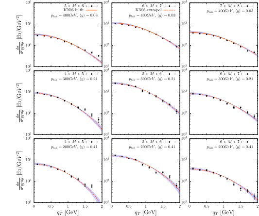
Figure 1: Theoretical predictions obtained with the KN05 model KN05 compared to DY transverse momentum spectra in $pA$ collisions Ito in bins of the invariant mass of the pair, $M$, expressed in GeV, for different incident beam energies and DY pairs rapidities. Solid lines indicate predictions in the phase space region included in the KN05 fit whereas dashed ones indicate predictions in an extrapolation regime. The error band corresponds to the $a_{i}^{\prime}s$ error propagation.

The latter is parametrised as

$$S_{NP}^{pp}(b)=\exp\{-[a_{1}+a_{2}\ln(M/(3.2\,\mbox{GeV}))+a_{3}\ln(100x_{1}x_{2})]b^{2}\}\,.$$ (12)

The $a_{i}$ parameters appearing in Eq. (12) are determined by a minimisation procedure against data and are given by KN05

$$a_{1}=0.201\pm 0.011,\;\;a_{2}=0.184\pm 0.018,\;\;a_{3}=-0.026\pm 0.007\,.$$ (13)

The fit is fully specified once a prescription for the treatment of the non perturbative, large-$b$, region both in the Sudakov form factor, Eq. (6), and the parton distributions is given. The authors of Ref. KN05 adopt the so-called $b_{\star}$-prescription, substituting $b$ with

$$b_{\star}(b,b_{max})=\frac{b}{\sqrt{1+\Big{(}\frac{b}{b_{max}}\Big{)}^{2}}}\,,$$ (14)

and setting $b_{max}=1.5\,\mbox{GeV}^{-1}$ in the perturbative form factor. In principle, the same setting should be used in PDFs, which are evaluated at the factorisation scale $\mu_{F}=b_{0}/b_{*}$. However this choice for $b_{max}$ may imply a call to a specific PDFs parameterization below their lowest available scale, $Q_{in}$. Since in Ref. KN05 cross sections are evaluated with the NLO CTEQ6M PDFs CTEQ6 , whose lowest $Q$ accessible is $Q_{in}=1.3$ GeV, the $b_{\star}$-prescription entering PDFs calls is used with $b_{max}=b_{0}/Q_{in}\simeq 0.86\,\mbox{GeV}^{-1}$ which always guarantees $\mu_{F}>Q_{in}$. It is important to remark that the non perturbative form factor is determined not only by fitting the parameters of the chosen functional form, but also by the specific regularisation prescription and its associated parameters adopted to deal with the infrared region. In general all these ingredients have been found to be highly correlated.

In order to present a benchmark of our code and to gauge how theory performs in extrapolation regions, we compare predictions from KN05 to the $pA$ data of Ref. Ito . An additional $\pm 25\%$ normalisation error is assigned to the data Ito . In the original KN05 analysis, only the data at $p_{lab}=400$ GeV, $q_{T}<1.4$ GeV, $5<M/\mbox{GeV}<9$ were included in the fit. In such a restricted region indeed the theory (solid lines) performs well offering a good benchmark of our code, as shown in the first row of Fig. 1. Since the $\pi W$ data to be analyzed in the following are at $p_{lab}$=252 GeV, it is important to check how well the theory performs in extrapolation regions at lower $\sqrt{s}$ and higher DY rapidity. Therefore we present in the second and third rows of Fig. 1 the KN05 benchmark (dashed lines) versus data Ito at $p_{lab}$= 200 and 300 GeV, which were not included in the KN05 fit. By using Eq. (4) and Eq. (5) and assuming the invariant mass values indicated on the plots, the rapidity coverage of these data can be converted to the range $0<x_{F}<0.3$. In both cases we find good agreement between data and theory up to $q_{T}\sim 2$ GeV giving us confidence that the KN05 model can be successfully used in this ($x_{F},q_{T}$) range at the $\sqrt{s}$ of interest in this analysis.

II.3 Pion structure

A calculation of pion TMDs in a NJL framework, with Pauli-Villars regularisation, has been recently presented in Ref. ns . Model calculations of meson partonic structure within this approach have a long story of successful predictions Davidson:2001cc ; Theussl:2002xp ; RuizArriola:2002bp ; Noguera:2011fv ; Weigel:1999pc ; Broniowski:2017gfp . Collinear parton distributions obtained within a model have to be associated to a low momentum scale $Q_{0}^{2}$ and, in order to be used to predict measured quantities, have to be evolved to higher momentum scales according to perturbative QCD (pQCD).

In Ref. ns the unpolarized NJL parton TMD has been obtained. Among its good properties, we stress that, upon integration over the intrinsic quark transverse momentum $\bm{k_{T}}$, the pion PDF $q(x)$ is properly recovered with correct normalisation and the momentum sum rule is exactly satisfied. This is due to the fact that NJL is a field theoretical scheme and the correct support of the PDF, $0\leq x\leq 1$, is not imposed but arises naturally. In particular, the momentum sum rule reads $\int dx~{}x~{}q\left(x\right)=0.5$, i.e. the fraction of momentum carried by each quark is one half of the total momentum, since at the scale of the model only valence quarks are present. The dependence on $\bm{k_{T}}$ of the TMD obtained in Ref. ns is very important for the present study. It is worth stressing that, in this approach, the $\bm{k_{T}}$ dependence is automatically generated by the NJL dynamics and it is not imposed by using any educated guess. This is an important feature of the results of Ref. ns , not found in other approaches Frederico:2009fk ; Pasquini:2014ppa . In this paper we will use the pion TMD obtained in Ref. ns in the chiral limit, which is an excellent approximation to the NJL full result; this is very convenient in the present calculation, since, at the low but undetermined scale $Q_{0}^{2}$ associated to the model, the pion TMD can be written in a factorised form

$$f^{q/\pi}(x_{\pi},\bm{k_{T}},Q_{0}^{2})=q(x_{\pi},Q_{0}^{2})T(\bm{k_{T}})~{},$$ (15)

where one has (in $\pi^{-}$, of interest here):

$$q(x_{\pi},Q_{0}^{2})=d_{v}(x_{\pi},Q_{0}^{2})=\bar{u}(x_{\pi},Q_{0}^{2})=1\,.$$ (16)

The function $T$ is given by

$$T(\bm{k_{T}})=\frac{3}{4\pi^{3}}{\left(m\over f_{\pi}\right)^{2}}~{}\sum_{i=0,2}\frac{c_{i}}{k_{T}^{2}+m_{i}^{2}}\,,$$ (17)

which, due to a proper combination of the $c_{i}$ ns , behaves as $k_{T}^{-6}$ for asymptotic values of $k_{T}=|\bm{k_{T}}|$ and satisfies the normalisation

$$\int d^{2}\bm{k_{T}}\,T(\bm{k_{T}})=1\,.$$ (18)

Since the distribution Eq. (17) depends only upon $k_{T}^{2}$, its Fourier transform can be cast in the form

$$S_{NP}^{\pi}(b) = \frac{3}{2\pi^{2}}{\left(m\over f_{\pi}\right)^{2}}~{}\sum_{i=0,2}\int\,dk_{T}\,k_{T}\,J_{0}(bk_{T})\frac{c_{i}}{k_{T}^{2}+m_{i}^{2}}$$ (19)

$$= \frac{3}{2\pi^{2}}{\left(m\over f_{\pi}\right)^{2}}~{}\sum_{i=0,2}c_{i}K_{0}(m_{i}\,b)\,,$$

where $K_{0}$ is the modified Bessel function of the second kind. The parameters used in Eq. (19) are given in Ref. ns and read

$$m_{0}^{2}=m^{2}=(0.238\;\mbox{GeV})^{2},\quad m_{1}^{2}=m^{2}+\Lambda^{2},\quad m_{2}^{2}=m^{2}+2\Lambda^{2}$$

$$\Lambda=0.860\;\mbox{GeV},\quad c_{0}=1,\quad c_{1}=-2,\quad c_{2}=1,\quad f_{\pi}=0.0924\;\mbox{GeV}\,.$$

As noted above, the NJL pion model corresponds to a low hadronic scale $Q_{0}^{2}$. Such a low scale has been determined previously by directly comparing the second moment of the pion PDF evaluated in NJL model with the results from the analysis of Ref. Sutton:1991ay . The procedure gives a value of $Q_{0}^{2}=0.18$ GeV² at NLO Courtoy:2008nf ; CourtoyThesis .

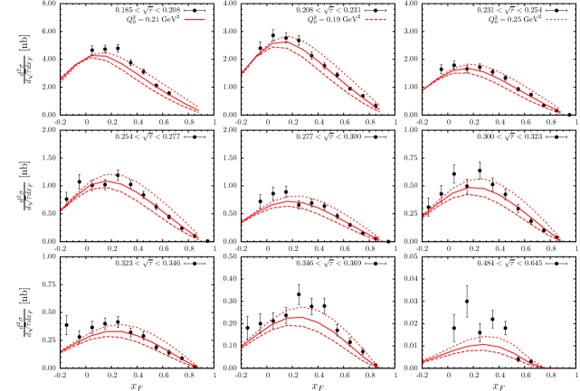
Figure 2: Drell-Yan pairs production in $\pi^{-}W$ collisions. Next-to-leading order cross sections obtained by using evolved NJL pion PDFs for three values of $Q_{0}^{2}$ are compared to data of Ref. conway .

In the present paper we use a different strategy : we consider $Q_{0}^{2}$ a free parameter of the NJL model which is then fixed with a minimisation procedure, outlined in the following, of the theoretical $\pi^{-}W$ DY cross sections, differential in $\sqrt{\tau}$ and $x_{F}$, against the corresponding experimental ones  conway . Theoretical cross sections are calculated according to

$$\frac{d^{2}\sigma}{dQ^{2}dx_{F}}=\frac{4\pi\alpha_{em}^{2}}{9Q^{2}s}\sum_{ij}e_{i}^{2}\int_{x_{1}}^{1}dt_{1}\int_{x_{2}}^{1}dt_{2}\frac{d^{2}\hat{\sigma}^{ij}}{dQ^{2}dx_{F}}f_{i/\pi}(t_{1},Q^{2})f_{j/p}(t_{2},Q^{2})\,,$$ (20)

where the partonic cross sections $d\hat{\sigma}^{ij}$ are calculated at NLO accuracy by using the results of Ref. Sutton:1991ay . An additional correction takes into account the correct number of gluon polarisations in the $\overline{\mbox{MS}}$ in dimensional regularisation Aicher:2010cb . The NJL pion PDFs are evolved to NLO accuracy in the Variable Flavor Number Scheme, with the initial condition given in Eq. (16), with the help of the QCDNUM QCDNUM evolution code. The QCD parameters are those of the NLO CTEQ6M parameterisation CTEQ6 . In particular we set the NLO running coupling to $\alpha_{s}^{(n_{f}=5)}(M_{Z})=0.118$ at the $Z$-boson mass, $M_{Z}$. Since the data we are comparing to are obtained on a tungsten target, we take into account nuclear effects by using nuclear PDFs of Ref. nCTEQ . We have carried out a $\chi^{2}$ study to establish the hadronic scale of the model that describes the best the data at NLO in pQCD. Two cases have been considered: an evaluation of the $\chi^{2}$ for the full range of $x_{F}$ and another one with a cut $x_{F}<0.4$, since the NJL model is expected to better reproduce the pion valence distributions, expected to populate the range of large and positive $x_{F}$ . The scales thus determined are

$$Q_{0,\,\mbox{\tiny no cut}}^{2}=0.212_{-0.012}^{+0.011}\;\mbox{GeV}^{2},\quad\quad Q_{0,\,\mbox{\tiny cut}}^{2}=0.209_{-0.009}^{+0.008}\;\mbox{GeV}^{2},$$ (21)

and correspond to a chisquare value of $\chi^{2}/$d.o.f.$=2.1$ and $1.9$, respectively. The quoted errors correspond to a variation of one unit in $\chi^{2}$, i.e. 1-$\sigma$. Those results are compatible with each other. We will therefore refer to $Q_{0}^{2}=0.21$ GeV², as the scale associated to the pion NJL model. The other two curves in Fig. 2, corresponding to $Q_{0}^{2}=0.19$ GeV² and $Q_{0}^{2}=0.25$ GeV² respectively, are added, in order to show the sensitivity to this particular choice of infrared $Q_{0}^{2}$. It is worth noticing that the results show an acceptable agreement, both in shape and in normalisation. More in detail, a tendency of the theory to undershoot the data is identified in the range of small $x_{F}$ ($-0.2<x_{F}<0.2$). This deficiency is not unexpected since, in the mentioned kinematic region, the dominant contribution to the cross sections involves sea quarks and gluons which are absent at $Q_{0}^{2}$ and are radiatively generated by QCD evolution. This is a typical drawback of models which contain only valence contributions at the hadronic scale. At this point we would like to mention that the theoretical description of the $x_{F}$-spectra at large $x_{F}$ and the determination of pion parton distributions can be further improved employing resummation techniques presented in Ref. Aicher:2010cb ; Aicher:2011ai ; Westmark:2017uig . It is worth noticing that, as shown in those papers, threshold NLL resummation of the Wilson coefficients leads to larger cross sections at large $x$ with respect to NLO ones. This, in turn, implies softer pion PDFs at large $x$. In the present context, this fact would imply a scale $Q_{0}^{2}$ for the NJL model lower than the one already determined by using NLO Wilson coefficients in Eq. (20).

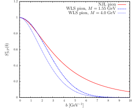
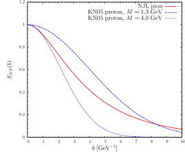
Figure 3: Transverse profile in $b$-space for the NJL pion, eq. (19), compared, in the left panel, to WLS pion Wang:2017zym and, in the right panel, to the KN05 proton, $\sqrt{S_{NP}^{pp}(b)}$, both evaluated for different values of the scale $M$.

III Predictions for $\pi W$ collisions data

Predictions for the $\pi W$ Drell-Yan cross sections are obtained once appropriate modifications are implemented in Eq. (2). Evolved NJL pion parton distributions replace proton PDFs for hadron 1. Moreover the non-perturbative form factor $S_{NP}^{h_{1}h_{2}}(b)$ depends on the particle species initiating the reaction. Therefore in $\pi W$ collisions the latter is written as follows:

$$S_{NP}^{\pi W}(b)=S_{NP}^{\pi}(b)\,\sqrt{S_{NP}^{pp}(b)}\,,$$ (22)

where $S_{NP}^{\pi}(b)$ is given in Eq. (19) and the square root on $S_{NP}^{pp}(b)$, given in Eq. (12), takes into account that now only one proton is involved in the process. It is instructive to directly compare the proton and pion non perturbative transverse distributions used in the calculation. It is important to remark that the NJL pion transverse distribution in Eq. (19) differs from the corresponding proton factor in Eq. (12) in that it does not contain any explicit dependence neither on hard scale $M$ nor on parton fractional momenta. Such a comparison is meaningful at the typical scale for which the transverse form factors and the longitudinal momentum part factorize. For the pion case this happens at the scale $Q_{0}^{2}$ determined in the previous section. For the proton TMD such a scale is ambiguously defined and, according to KN05 analysis, ranges between $Q_{in}^{2}$ and $(b_{0}/b_{max}^{KN05})^{2}$. Therefore we choose $M=Q_{in}=1.3$ GeV in Eq. (12) and fix the product $x_{1}x_{2}=M^{2}/s$, see Eq. (4), exploiting the $\pi^{-}W$ kinematics with $s$ calculated according to a beam energy of $p_{lab}=252$ GeV. The comparison is presented in Fig. 3. All the distributions reduce to unity in the $b\rightarrow 0$ limit, since they are all normalised to unity in transverse momentum space. In the left panel of Fig. 3 we compare the NJL transverse distribution to the pion parametrisation of Ref. Wang:2017zym (called hereafter WLS) obtained from a fit of the same cross section data used in the present paper. One may notice that, for this model, the width of the distribution is smaller with respect to the NJL one, implying a larger average transverse momentum. In the right panel of Fig. 3 one may notice that the NJL pion transverse distribution develops a larger tail with respect to the gaussian drop of the proton distributions. Moreover the $b$-space width of the KN05 proton with $M=1.3$ GeV is larger with respect to the pion one. When transformed back in $k_{T}$ space, this implies that the intrinsic transverse momentum in the pion is larger than the one in the proton, in agreement with the general expectations, since the pion is a much smaller system with respect to the proton. It is worth mentioning that both the KN05 and WLS non perturbative form factors have an explicit, althought slightly different, dependence upon the hard scale $M$, in both cases set equal to the invariant mass of the dilepton pair. Therefore we plot in each panels, as a representative case, the curves corresponding to both form factors evaluated with the scale set to $M=4$ GeV. Comparing the latter curves to the ones with $M\sim 1$ GeV, we conclude that the $M$-dependence generates a sizable non perturbative evolution of the form factor which is more pronounced for KN05 proton model than for the WLS pion model.

We now turn to the discussion of the perturbative part of the Sudakov form factor, Eq. (6). The latter, at variance with its non perturbative counter part, does not depend upon the type of initial state hadrons involved in the scattering process. In principle, the same regularisation procedure should be used both in the Sudakov and in the PDFs. This optimum indeed faces some technical problem, for example the call to PDFs to values outside the boundary of the grid in which they are defined and the different scales at which the transverse distributions are assumed to factorise on the proton and pion side, respectively. In order to accomodate all these different settings, we find useful to split the perturbative form factor in Eq. (6) in a form which allows to use distinct $b_{max}$ on the proton and pion side:

$$S_{q}(Q,b) \equiv S_{q}(Q,b_{*},b_{max}^{p},b_{max}^{\pi})$$ (23)

$$= \exp\left\{-\frac{1}{2}\int_{\frac{b_{0}^{2}}{b^{2}_{*}(b_{max}^{p})}}^{Q^{2}}\frac{dq^{2}}{q^{2}}\left[A(\alpha_{s}(q^{2}))\;\ln\frac{Q^{2}}{q^{2}}+B(\alpha_{s}(q^{2}))\right]\right\}\,$$

$$\times\exp\left\{-\frac{1}{2}\int_{\frac{b_{0}^{2}}{b^{2}_{*}(b_{max}^{\pi})}}^{Q^{2}}\frac{dq^{2}}{q^{2}}\left[A(\alpha_{s}(q^{2}))\;\ln\frac{Q^{2}}{q^{2}}+B(\alpha_{s}(q^{2}))\right]\right\}\,.$$

For the proton parameters, we stick to KN05 settings since the $a_{i}$’s in Eq. (12) optimized for $b_{max}^{p}=1.5$ Ge$\mbox{V}^{-1}$. On the pion side there is some freedom in adjusting $b_{max}^{NJL}$. However the pion TMD shows a $x-k_{T}$ factorised structure only at $Q_{0}^{2}$, whose numerical value has been determined in the previous section. Therefore we can expect the $b_{*}$-prescription to involve $b_{max}^{\pi}$ values of the order $b_{0}/Q_{0}\sim 2.44$ Ge$\mbox{V}^{-1}$, which will be our default value to be used both in the Sudakov and in NJL pion parton distributions regularisation.

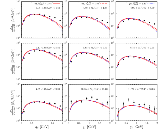
Figure 4: Predictions compared to cross sections in various invariant mass bins of the pair integrated in $0<x_{F}<1$. Data from Refs. conway ; stirling

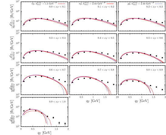
Figure 5: Predictions compared to differential cross sections in various $x_{F}$ bins integrated in the mass range $4<M<8.55$ GeV. Data from Refs. conway ; stirling

We now turn to the comparison to lepton pair $q_{T}$-spectra collected in tables D92-D97 of Refs. conway ; stirling , measured in $\pi W$ collisions. Such data actually refer to less differential cross sections with respect to the one appearing in Eq. (2). In this case differential cross sections are integrated over additional variables according to values specified in experimental analyses. We start presenting our results showing, in Fig. 4, cross sections differential in $q_{T}$ integrated in $0<x_{F}<1$ in various bins of the invariant mass of the pair, $M$. The comparison is performed up to a $q_{T}\sim 2$ GeV, where we have checked that the KN05 gives an adequate description of $pp$ data. All three different predictions, to be discussed in the following, capture the normalisation of the data and share a tendency to slightly overestimate the data at very small $q_{T}$ and to underestimate them at larger $q_{T}$. This effect progressively disappears increasing the mass of the lepton pair. Comparing the two curves corresponding to $b_{max}^{NJL}=2.44$ Ge$\mbox{V}^{-1}$ and $b_{max}^{NJL}=1.5$ Ge$\mbox{V}^{-1}$, one may notice a substantial stability upon variation of the regulators on the pion side. On the same plot, in order to investigate the sensitivity to the pion transverse distribution, we additionally show the predictions obtained by substituting the pion transverse factor, Eq. (19), with $\sqrt{S_{NP}^{pp}(b)}$. As shown in Fig. 3, the non perturbative transverse distributions for the proton and pion differ at low scales. The corresponding curve, indicated with $pp$ on the plot, is barely distinguishable from the other two. Such a comparison supports the hypothesis that the effect of the perturbative evolution, driven by Eq. (23), is to wash away differences in the non perturbative structure found at the hadronic scale. This result implies a reduced sensitivity to non perturbative structure. We proceed our discussion presenting in Fig. 5 the comparison between theory predictions against the same data, now integrated in the mass range $4<M<8.55$ GeV in a number of $x_{F}$ bins. We remind the reader that we have verified that the KN05 model gives a satisfactory description of $pp$ data up to $x_{F}\sim 0.3$. Up to this $x_{F}$ value, as shown in the first row of Fig. 5, the description $\pi^{-}W$ data is fair, as already observed in Fig. 4. Beyond that range, however, the width of the theoretical curves decreases more rapidly than observed in the data, with data substantially undershooted beyond $q_{T}\sim 1$ GeV. This effect is more pronounced as $x_{F}$ increases. In this region of relatively large pion fractional momenta it would be tempting to invoke, in order to describe the data, an $x$-dependent non perturbative structure. Such an interesting hypothesis, however, cannot be tested unless fixed order contributions at finite $q_{T}$ are included in the calculation. On the other hand we notice that the WLS pion model of Ref. Wang:2017zym , which does not include any additional $x_{i}$ dependence in the non perturbative form factor, is able to reproduce the data up to $x_{F}\sim 0.8$. On the theoretical side, we would like to mention that, in this range of quite large pion parton fractional momenta, the theoretical description of the $q_{T}$-spectrum can be further improved employing joint resummation techniques described in Refs. Kulesza:2002rh ; Muselli:2017bad . In order to better appreciate how the width of theoretical predictions evolves with $x_{F}$ (and therefore with $x_{\pi}$) and the invariant mass of the lepton pair, we show in Fig. 6 the average transverse momentum of the pair, $\langle q_{T}^{2}\rangle$, calculated as

$$\langle q_{T}^{2}\rangle=\frac{\displaystyle\int_{x_{F}^{\mbox{\tiny min}}}^{x_{F}^{\mbox{\tiny max}}}dx_{F}\int_{\tau_{\mbox{\tiny min}}}^{\tau_{\mbox{\tiny max}}}d\tau\int_{0}^{q_{T}^{2,\mbox{\tiny max}}}dq_{T}^{2}\;q_{T}^{2}\;\frac{d^{3}\sigma}{dx_{F}d\tau dq_{T}^{2}}}{\displaystyle\int_{x_{F}^{\mbox{\tiny min}}}^{x_{F}^{\mbox{\tiny max}}}dx_{F}\int_{\tau_{\mbox{\tiny min}}}^{\tau_{\mbox{\tiny max}}}d\tau\int_{0}^{q_{T}^{2,\mbox{\tiny max}}}dq_{T}^{2}\;\frac{d^{3}\sigma}{dx_{F}d\tau dq_{T}^{2}}}\,.$$ (24)

Integration limits are provided by experimental conditions.

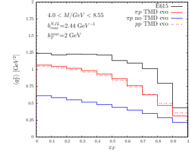
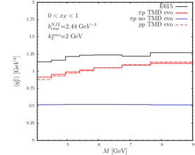
Figure 6: Left panel: lepton pair average transverse momentum, $\langle q_{T}^{2}\rangle$, as a function of $x_{F}$ integrated in the mass range $4.0<M/$GeV$<8.55$. Right panel: $\langle q_{T}^{2}\rangle$ as a function of $M$ integrated in the range $0<x_{F}<1$. Averaged values are obtained integrating both predictions and the phenomenological parametrisation of the data up to $q_{T}^{max}=2$ GeV.

For data, indicated by black lines in Fig. 6, the phenomenological parametrisation presented in Ref. conway is used. For both theory and data, the $\langle q_{T}^{2}\rangle$ is calculated with a maximum value of $q_{T}^{max}=2$ GeV. Theory predictions tend to undershoot the data but, overall, a good shape agreement is found. By comparing lines with and without TMD evolution (for the latter the perturbative Sudakov $S_{q}$ is removed from the evaluation of Eq. (2)) one can appreciate its large impact on the amount of generated $\langle q_{T}\rangle$. On the same plot, in order to investigate the sensitivity to the pion transverse structure, we additionally show the predictions obtained by substituting the pion transverse factor, Eq. (19), with $\sqrt{S_{NP}^{pp}(b)}$. As already seen in Fig. 4, differences are minimal, implying a reduced sensitivity to details of the non perturbative transverse factor. Therefore if one aims to better appreciate the strictly non perturbative form factor, one has to confine in corners where TMD evolution is minimised, but still in a perturbative range. These phase space regions can be identified by extrapolation from the right plot as the one at the lowest, but still perturbative, values of the invariant masses of the pair.

IV Conclusions

A thorough analysis of DY pair production in pion-nucleus scattering has been presented. The main goal of our work has been the test of model predictions, obtained within the Nambu–Jona-Lasinio model for the transverse pion structure. In particular we have focused on the study of differential transverse momentum spectra of DY pairs produced in $pA$ collisions calculated in the CSS framework at NLL accuracy borrowing from the literature the longitudinal and transverse proton structure. The pion is treated in the Nambu-Jona–Lasinio model. No further assumption has been made: even the momentum scale associated to the model is obtained via a minimization procedure of NLO theory to DY experimental longitudinal spectra. The latter turns out to be a low one, in line with that normally used, which could be predicted within the spirit of the model without fitting “a posteriori”. The agreement found between our pion-nucleus theoretical cross sections and experimental data is rather successful, confirming the predictive power of the NJL model, for both the longitudinal pion parton distributions and its transverse structure. We notice that the theory tends to systematically undershoot the data on the higher end of the considered $q_{T}$ interval. All interpretations of this effect, however, are not conclusive without the inclusion of the finite, fixed order, contributions which populate the $q_{T}\sim Q$ region and are neglected in our calculation.

The possibility to distinguish between different non perturbative transverse momentum distributions in DY data appears instead more questionable. In this complicated scenario, a possible strategy would be the measurement of DY pion-nucleus $q_{T}$-spectra, in bins of $x_{F}$, at low values of the mass of the pair, as the present study suggests to look into this kinematical window to emphasize the non-perturbative content of the pion. Further analyses of the pion non-perturbative form factor, as a function of the hard scale, should be pursued so we could progress on that point. In the very same window, new data could allow a deeper investigation of the dependence of the non perturbative form factor upon the hard scale of the process.

References

- (1) S. D. Drell and T. M. Yan, Phys. Rev. Lett. 25 (1970) 316 Erratum: [Phys. Rev. Lett. 25 (1970) 902]. doi:10.1103/PhysRevLett.25.316, 10.1103/PhysRevLett.25.902.2
- (2) M. Diehl, Eur. Phys. J. A 52 (2016) no.6, 149 doi:10.1140/epja/i2016-16149-3 [arXiv:1512.01328 [hep-ph]].
- (3) Y. L. Dokshitzer, D. Diakonov and S. I. Troian, Phys. Rept. 58 (1980) 269. doi:10.1016/0370-1573(80)90043-5
- (4) G. Parisi and R. Petronzio, Nucl. Phys. B 154 (1979) 427. doi:10.1016/0550-3213(79)90040-3
- (5) G. Altarelli, R. K. Ellis, M. Greco and G. Martinelli, Nucl. Phys. B 246 (1984) 12. doi:10.1016/0550-3213(84)90112-3
- (6) J. C. Collins, D. E. Soper and G. F. Sterman, Nucl. Phys. B 250 (1985) 199. doi:10.1016/0550-3213(85)90479-1
- (7) G. Bozzi, S. Catani, G. Ferrera, D. de Florian and M. Grazzini, Nucl. Phys. B 815 (2009) 174 doi:10.1016/j.nuclphysb.2009.02.014 [arXiv:0812.2862 [hep-ph]].
- (8) G. Bozzi, S. Catani, G. Ferrera, D. de Florian and M. Grazzini, Phys. Lett. B 696 (2011) 207 doi:10.1016/j.physletb.2010.12.024 [arXiv:1007.2351 [hep-ph]].
- (9) S. Catani, D. de Florian, G. Ferrera and M. Grazzini, JHEP 1512 (2015) 047 doi:10.1007/JHEP12(2015)047 [arXiv:1507.06937 [hep-ph]].
- (10) S. Catani, D. de Florian and M. Grazzini, Nucl. Phys. B 596 (2001) 299 doi:10.1016/S0550-3213(00)00617-9 [hep-ph/0008184].
- (11) D. de Florian and M. Grazzini, Phys. Rev. Lett. 85 (2000) 4678 doi:10.1103/PhysRevLett.85.4678 [hep-ph/0008152]
- (12) A. V. Konychev and P. M. Nadolsky, Phys. Lett. B 633 (2006) 710 doi:10.1016/j.physletb.2005.12.063 [hep-ph/0506225].
- (13) F. Landry, R. Brock, P. M. Nadolsky and C. P. Yuan, Phys. Rev. D 67 (2003) 073016 doi:10.1103/PhysRevD.67.073016 [hep-ph/0212159].
- (14) S. M. Aybat and T. C. Rogers, Phys. Rev. D 83 (2011) 114042 doi:10.1103/PhysRevD.83.114042
- (15) I. Scimemi and A. Vladimirov, Eur. Phys. J. C 78 (2018) no.2, 89 doi:10.1140/epjc/s10052-018-5557-y [arXiv:1706.01473 [hep-ph]].
- (16) A. Bacchetta, F. Delcarro, C. Pisano, M. Radici and A. Signori, JHEP 1706 (2017) 081 doi:10.1007/JHEP06(2017)081 [arXiv:1703.10157 [hep-ph]].
- (17) P. Sun, J. Isaacson, C.-P. Yuan and F. Yuan, Int. J. Mod. Phys. A 33 (2018) no.11, 1841006 doi:10.1142/S0217751X18410063 [arXiv:1406.3073 [hep-ph]].
- (18) F. A. Ceccopieri and L. Trentadue, Phys. Lett. B 741 (2015) 97 doi:10.1016/j.physletb.2014.12.024 [arXiv:1407.7972 [hep-ph]].
- (19) A. Prokudin, P. Sun and F. Yuan, Phys. Lett. B 750 (2015) 533 doi:10.1016/j.physletb.2015.09.064 [arXiv:1505.05588 [hep-ph]].
- (20) P. Chiappetta and M. Greco, Nucl. Phys. B199 (1982) 77. doi:10.1016/0550-3213(82)90567-3
- (21) T. Frederico, E. Pace, B. Pasquini and G. Salme, Phys. Rev. D 80 (2009) 054021 doi:10.1103/PhysRevD.80.054021 [arXiv:0907.5566 [hep-ph]].
- (22) B. Pasquini and P. Schweitzer, Phys. Rev. D 90 (2014) no.1, 014050 doi:10.1103/PhysRevD.90.014050 [arXiv:1406.2056 [hep-ph]].
- (23) X. Wang, Z. Lu and I. Schmidt, JHEP 1708 (2017) 137 doi:10.1007/JHEP08(2017)137 [arXiv:1707.05207 [hep-ph]].
-
(24)
COMPASS collaboration, F. Gautheron et al.,
wwwcompass.cern.ch/compass/proposal/compass-II_proposal/compass-II_proposal.pdf - (25) M. Engelhardt, P. Hägler, B. Musch, J. Negele and A. Schäfer, Phys. Rev. D 93 (2016) no.5, 054501 doi:10.1103/PhysRevD.93.054501 [arXiv:1506.07826 [hep-lat]].
- (26) B. U. Musch, P. Hagler, M. Engelhardt, J. W. Negele and A. Schafer, Phys. Rev. D 85 (2012) 094510 doi:10.1103/PhysRevD.85.094510 [arXiv:1111.4249 [hep-lat]].
- (27) Z. Lu and B. Q. Ma, Phys. Rev. D 70 (2004) 094044 doi:10.1103/PhysRevD.70.094044 [hep-ph/0411043].
- (28) L. Gamberg and M. Schlegel, Phys. Lett. B 685 (2010) 95 doi:10.1016/j.physletb.2009.12.067 [arXiv:0911.1964 [hep-ph]].
- (29) Z. Lu, B. Q. Ma and J. Zhu, Phys. Rev. D 86 (2012) 094023 doi:10.1103/PhysRevD.86.094023 [arXiv:1211.1745 [hep-ph]].
- (30) S. Noguera and S. Scopetta, JHEP 1511 (2015) 102 doi:10.1007/JHEP11(2015)102 [arXiv:1508.01061 [hep-ph]].
- (31) A. Bacchetta, S. Cotogno and B. Pasquini, Phys. Lett. B 771 (2017) 546 doi:10.1016/j.physletb.2017.05.072 [arXiv:1703.07669 [hep-ph]].
- (32) S. P. Klevansky, Rev. Mod. Phys. 64 (1992) 649. doi:10.1103/RevModPhys.64.649
- (33) M. Aghasyan et al. [COMPASS Collaboration], Phys. Rev. Lett. 119 (2017) no.11, 112002 doi:10.1103/PhysRevLett.119.112002 [arXiv:1704.00488 [hep-ex]].
- (34) J. Kodaira and L. Trentadue, Phys. Lett. 112B (1982) 66. doi:10.1016/0370-2693(82)90907-8
- (35) C. T. H. Davies and W. J. Stirling, Nucl. Phys. B 244 (1984) 337. doi:10.1016/0550-3213(84)90316-X
- (36) J. Pumplin, D. R. Stump, J. Huston, H. L. Lai, P. M. Nadolsky and W. K. Tung, JHEP 0207 (2002) 012 doi:10.1088/1126-6708/2002/07/012 [hep-ph/0201195].
- (37) A. S. Ito et al., Phys. Rev. D 23 (1981) 604. doi:10.1103/PhysRevD.23.604
- (38) R. M. Davidson and E. Ruiz Arriola, Acta Phys. Polon. B 33 (2002) 1791 [hep-ph/0110291].
- (39) L. Theussl, S. Noguera and V. Vento, Eur. Phys. J. A 20 (2004) 483 doi:10.1140/epja/i2003-10174-3 [arXiv:nucl-th/0211036].
- (40) E. Ruiz Arriola and W. Broniowski, Phys. Rev. D 66 (2002) 094016 doi:10.1103/PhysRevD.66.094016 [arXiv:hep-ph/0207266].
- (41) S. Noguera and S. Scopetta, Phys. Rev. D 85 (2012) 054004 doi:10.1103/PhysRevD.85.054004 [arXiv:1110.6402 [hep-ph]].
- (42) H. Weigel, E. Ruiz Arriola and L. P. Gamberg, Nucl. Phys. B560 (1999) 383 doi:10.1016/S0550-3213(99)00426-5 [hep-ph/9905329].
- (43) W. Broniowski and E. Ruiz Arriola, Phys. Rev. D 97 (2018) no.3, 034031 doi:10.1103/PhysRevD.97.034031 [arXiv:1711.03377 [hep-ph]].
- (44) J. S. Conway et al., Phys. Rev. D 39 (1989) 92. doi:10.1103/PhysRevD.39.92
- (45) A. Courtoy and S. Noguera, Phys. Lett. B 675 (2009) 38 doi:10.1016/j.physletb.2009.03.070 [arXiv:0811.0550 [hep-ph]].
- (46) A. Courtoy, Ph. D. Thesis, Valencia University, 2009. http://arxiv.org/abs/arXiv:1010.2974
- (47) S. Noguera and V. Vento, Eur. Phys. J. A 28 (2006) 227 doi:10.1140/epja/i2006-10045-5 [hep-ph/0505102].
- (48) P. J. Sutton, A. D. Martin, R. G. Roberts and W. J. Stirling, Phys. Rev. D 45 (1992) 2349. doi:10.1103/PhysRevD.45.2349
- (49) M. Aicher, A. Schafer and W. Vogelsang, Phys. Rev. Lett. 105 (2010) 252003 doi:10.1103/PhysRevLett.105.252003 [arXiv:1009.2481 [hep-ph]].
- (50) M. Botje, Comput. Phys. Commun. 182 (2011) 490 doi:10.1016/j.cpc.2010.10.020 [arXiv:1005.1481 [hep-ph]].
- (51) K. Kovarik et al., Phys. Rev. D 93 (2016) no.8, 085037 doi:10.1103/PhysRevD.93.085037 [arXiv:1509.00792 [hep-ph]].
- (52) M. Aicher, A. Schafer and W. Vogelsang, Phys. Rev. D 83 (2011) 114023 doi:10.1103/PhysRevD.83.114023 [arXiv:1104.3512 [hep-ph]].
- (53) D. Westmark and J. F. Owens, Phys. Rev. D 95 (2017) no.5, 056024 doi:10.1103/PhysRevD.95.056024 [arXiv:1701.06716 [hep-ph]].
- (54) W. J. Stirling and M. R. Whalley, J. Phys. G 19 (1993) D1. doi:10.1088/0954-3899/19/D/001
- (55) A. Kulesza, G. F. Sterman and W. Vogelsang, Phys. Rev. D 66 (2002) 014011 doi:10.1103/PhysRevD.66.014011 [hep-ph/0202251].
- (56) C. Muselli, S. Forte and G. Ridolfi, JHEP 1703 (2017) 106 doi:10.1007/JHEP03(2017)106 [arXiv:1701.01464 [hep-ph]].