Feeding the multitude: A polynomial-time algorithm to improve sampling

Abstract

A wide variety of optimization techniques, both exact and heuristic, tend to be biased samplers. This means that when attempting to find multiple uncorrelated solutions of a degenerate Boolean optimization problem a subset of the solution space tends to be favored while, in the worst case, some solutions can never be accessed by the algorithm used. Here we present a simple post-processing technique that improves sampling for any optimization approach, either quantum or classical. More precisely, starting from a pool of a few optimal configurations, the algorithm generates potentially new solutions via rejection-free cluster updates at zero temperature. Although the method is not ergodic and there is no guarantee that all the solutions can be found, fair sampling is typically improved. We illustrate the effectiveness of our method by improving the exponentially biased data produced by the D-Wave 2X quantum annealer [S. Mandrà et al.,Phys. Rev. Lett. 118, 070502 (2017)], as well as data from three-dimensional Ising spin glasses. As part of the study, we also show that sampling is improved when sub-optimal states are included and discuss sampling at a finite fixed temperature.

I Introduction

Optimization problems, even when restricted to discrete (binary) optimization, appear in many scientific disciplines and industrial applications and typically map directly onto spin-glass-like Hamiltonians Stein and Newman (2013); Lucas (2014). These problems are computationally hard to solve with current hardware, which has led to the design and construction of special-purpose analog quantum optimization machines, such as the D-Wave Systems Inc. quantum annealer. In parallel, the development of efficient classical optimization techniques to study these NP-hard problems has experienced a renaissance in recent years. Although many optimization techniques exist for solving such problems, generally the complexity is worse than polynomial in the size of the input. Therefore, it is of much interest to develop efficient approaches to more efficiently study these systems.

While exact optimization techniques that obtain the optimum of a cost function with guarantees are always desirable, these can typically only handle a small number of variables Van Beek (2006); Montanaro (2015); Mandrà et al. (2016). Even worse, for degenerate optimization problems they often return a single configuration minimizing the cost function Elf et al. (2001); Pardella and Liers (2008); Liers and Pardella (2010). Therefore, heuristics are the tool of choice, at the cost of obtaining the solution of an optimization problem with a finite success probability. It is therefore of much interest to develop techniques that increase the quality and variety of solutions delivered by heuristics, as well as improve the sampling of the solution space for degenerate optimization problems. In parallel, sampling of uncorrelated solutions at finite energy, as is needed, for example, in machine learning applications, is currently also of much importance Torlai and Melko (2016); Levit et al. (2017); Crawford et al. (2018).

In this paper we present a simple polynomial-time algorithm that can substantially improve the sampling of degenerate ground states for Ising-type Hamiltonians by starting from a subset of (suboptimal) configurations. This is of much importance when estimating the ground-state entropy in physical systems, counting problems in computer science such as #SAT and #Knapsack Jerrum et al. (1986); Gomes et al. (2008); Gopalan et al. (2011), and industrial applications such as SAT filters Weaver et al. (2014); Douglass et al. (2015). More precisely, if the starting pool for our method contains only ground-state configurations, our proposed method can potentially increase the variety of minimizing configurations at a cheaper cost than other (often very expensive) means. If low-energy configurations are also included in the pool, the proposed method can be used to find configurations with a lower energy and increase the probability of success to find the ground state. Finally, if a pool of configurations at a finite energy (or temperature) is given, our approach can be used to generate new, often uncorrelated configurations at similar energy (or temperature). As part of our analysis, here we demonstrate how fair sampling Moreno et al. (2003); Matsuda et al. (2009); Mandrà et al. (2017) of states generated with transverse-field quantum annealing Finnila et al. (1994); Kadowaki and Nishimori (1998); Brooke et al. (1999); Farhi et al. (2001); Santoro et al. (2002); Das and Chakrabarti (2005); Santoro and Tosatti (2006); Das and Chakrabarti (2008); Morita and Nishimori (2008) using a D-Wave 2X quantum annealer com (a) can be improved.

We emphasize that the presented approach does not solve optimization problems in polynomial time, as this would mean that ${\rm P}={\rm NP}$, nor is it guaranteed to generate all solutions to a degenerate problem. Indeed, one has to first find a subset of solutions to jump-start the process and this task could be exponentially difficult. Nevertheless, a considerable amount of resources can be saved by generating a new set of solutions in polynomial time without the burden of running, e.g., time-consuming algorithms.

The paper is structured as follows. In Sec. II we present the algorithm as well as discuss potential areas where the approach could have considerable impact. Section III contains comprehensive benchmark results for different optimization problems as well as discusses the performance of the algorithm for nondegenerate optimization problems and sampling at finite temperature. Finally, Sec. IV summarizes our findings and presents an outlook for future directions.

II Algorithm and applications

In this section we first outline the algorithm, as well as variations on how to apply it to perform different tasks, followed by a selection of possible applications across disciplines.

II.1 Outline of the algorithm

The proposed algorithm is designed to perform large variable rearrangements on Ising-type Hamiltonians Yeomans (1992) (i.e., Boolean variables) with frustration. From a physics perspective, the most paradigmatic model systems ideally suited to be studied with this approach are spin glasses Binder and Young (1986); Stein and Newman (2013). However, because a plethora of discrete optimization problems can be mapped directly onto spin-glass-like Hamiltonians Hartmann and Rieger (2004); Lucas (2014), the method finds wide applicability across many disciplines.

Our polynomial-time algorithm is based on the cluster updates first introduced by Houdayer Houdayer (2001) for two-dimensional spin glasses and later generalized to systems of arbitrary topology by Zhu et al. Zhu et al. (2015). In its original incarnation, these cluster updates are combined with Monte Carlo sampling to ensure ergodicity and parallel tempering updates Geyer (1991); Hukushima and Nemoto (1996); Katzgraber et al. (2006) to either thermalize a system at a low, but finite temperature, or find optima for spin-glass-like Hamiltonians Moreno et al. (2003); Mandrà et al. (2016). Furthermore, the cluster updates can be used as accelerators for other optimization techniques, such as simulated annealing Kirkpatrick et al. (1983). Here we strip the Monte Carlo aspect from the algorithm and apply the cluster updates to variable configurations.

A cluster update is performed in the following way: First, compute the site overlap between two variable $s_{i}^{(1)}$ and $s_{i}^{(2)}$ at site $i$ of two different configurations $\{s^{(1)}\}$ and $\{s^{(2)}\}$, $q_{i}=s_{i}^{(1)}s_{i}^{(2)}$. This creates two domains in $q$ space with sites that have either $q_{i}=1$ or $q_{i}=-1$. Clusters are defined as the connected components of these domains. A randomly chosen site with $q_{i}=-1$ is used as the seed for a cluster that is built by adding all the connected variables in the $q_{i}=-1$ domain with probability $1$. This means the approach is rejection free. When no more sites can be added to the cluster, the variables in both configurations that correspond to the cluster in the overlap space where $q_{i}=-1$ are flipped with probability $1$, irrespective of their orientation.

It is important to note that, by construction, the combined change in energy $\Delta E$ (value of the cost function) is zero Houdayer (2001). However, in general the energy of one configuration will increase by an amount $\Delta E^{(1)}$, whereas the energy of the other configuration will decrease by the corresponding amount, i.e., $\Delta E^{(2)}=-\Delta E^{(1)}$. For the particular case of ground-state configurations, this means that $\Delta E^{(1)}=\Delta E^{(2)}=0$. As such, if two configurations are chosen from a pool of optima of a degenerate optimization problem, the resulting configurations will remain in the ground-state manifold.

Note that if clusters percolate (span the extent of the lattice) the cluster update does not produce two new configurations Houdayer (2001). However, in frustrated spin systems, it has been demonstrated Zhu et al. (2015) that cluster percolation is suppressed at low enough temperatures (energies) due to frustration. This means that in the study of low-energy states percolation should not affect the efficiency of the algorithm we outline below.

To generate new configurations out of a pool of existing configurations obtained by using any arbitrary heuristic, the algorithm randomly pairs two configurations from the pool, feeds them into the cluster update, and adds the resulting unique configurations back to the pool, unless these are already in the pool, in which case we increment the histogram. Therefore, the algorithm can be summarized as follows.

1. Start with a pool of ${\mathcal{C}}$ configurations computed with any simulational method.

2. Randomly select two configurations from the pool $\{s^{(n)}\}\in{\mathcal{C}}$, $n=\{1,2\}$.

3. Perform a Houdayer cluster update step using configurations $\{s^{(n)}\}$. If the resulting configurations $\{\tilde{s}^{(n)}\}\not\in{\mathcal{C}}$, add these new and unique solutions to the pool. If $\{\tilde{s}^{(n)}\}\in{\mathcal{C}}$, increase the count of this solution in the histogram.

4. Iterate as desired or until no new configurations can be found.

We emphasize that the algorithm is not ergodic. This means that there is no guarantee that, for example, all solutions to a degenerate optimization problem can be found. However, as illustrated in Sec. III below, the approach is quite efficient and for an increasing number of variables and/or problem degeneracy performs increasingly better while approaching a limiting distribution as discussed in the Appendix. Furthermore, the method can be used at finite temperature by feeding a pool of finite-temperature configurations to the cluster update.

There are several stopping criteria one can implement. For example, one can choose to stop when all solutions have been found, if they are known. However, this is typically not the case. Another approach is to stop when the empirical distribution of the accessible states is comparable to a distribution obtained by selecting from a uniform distribution (up to intrinsic statistical biases). While exhaustive enumeration of solutions rather than randomized flipping of domains can be a sensible approach, when applying this algorithm to random instances, we do not know the size of the solution manifold before starting the resampling. In addition, exhaustive enumeration of solutions does not scale for highly degenerate problems.

The success of the algorithm largely depends on the number of clusters in the initial pool of solutions. In this work the randomly generated instances we have used to benchmark the resampling method can have very different ground-state manifolds: some connected by a single spin flip or clusters composed of a single spin, as well as other larger clusters composed of multiple spins that equate to multiple spin flips. Should the initial set manifold consist of only spin-reversed ground states, the algorithm will not find new solutions or escape this particular region or regions of the ground-state manifold. In the case that there are more solutions to be found, this can be alleviated by adding excited states into the initial resampling pool. If such excited states are not readily available, they are easily generated by randomly flipping a fraction of variables in each ground-state configuration used in the initial solution pool.

II.2 Possible implementations

Note that any two configurations can be fed into the cluster update. Furthermore, the approach is easily parallelized on specialized hardware. Below we list possible ways in which the algorithm can be implemented with different goals in mind:

• (i)Expand the solution pool of a degenerate problem (ground states only). Start from a subset of solutions to a degenerate problem. Feeding the configurations to the cluster update could generate by design new ground-state configurations (if possible).

• (ii) Expand the solution pool of a degenerate problem (include low-energy states). Start from a pool of low-energy configurations and feed these to the cluster update. If the ground-state energy is known, keep track of all configurations that minimize the cost function. Although some solutions will be “lifted” from the ground-state manifold, having low-lying excited states vastly improves the sampling of the ground-state manifold.

• (iii) Improve solutions of both degenerate and nondegenerate optimization problems. Start from a pool of low-energy configurations and feed these to the cluster update. Keep track of the lowest cost-function values. In some cases, it is even possible to find the ground state for nondegenerate problems com (b).

• (iv) Sample solutions at a fixed but finite temperature (energy). Start from a pool of configurations computed at a given finite temperature (or average energy per spin) and feed these to the cluster algorithm. Keep track of the configurations whose energy falls within a desired energy window. Add the new configurations to the pool.

The aforementioned implementations illustrate a handful of ways the heuristic can be used to sample states of discrete optimization problems. We note that, quite often, the computational effort to generate the initial pool of states is sizable, especially for NP-hard problems, and as such, having a simple heuristic that can generate new configurations in polynomial time could be transformative for a very broad set of applications. In particular, for fully connected graphs, the presented approach scales as $O(N^{2})$, where $N$ is the size of the input.

II.3 Application scope

Because both ground-state and excited-state configurations can be used and because the cluster update can generate new configurations from existing states with potentially large Hamming distances if existing states with large Hamming distances are used, the approach finds wide applicability across disciplines. We list some application domains below. However, we emphasize that the method can be applied to any optimization problem where an overlap between two configurations can be constructed and where the interactions are symmetric, such as for a quadratic or higher-order unconstrained optimization problem.

• (i) Improving data quality in, e.g., quantum annealing machines. Because quantum annealers such as the D-Wave Systems Inc. devices perform the optimization step several times to improve the success probability of the solutions, a subset of obtained low-energy configurations can be fed into the cluster update to generate lower-energy solutions or thus increase success probabilities.

• (ii) Improving fair sampling for biased samples. It has been demonstrated Matsuda et al. (2009); Mandrà et al. (2017) that transverse-field quantum annealing is a biased sampling approach. Using the cluster update, the solution pool can be expanded and the biased sampling mitigated.

• (iii) Fast generation of uncorrelated solutions for SAT membership filters. — Probabilistic SAT membership filters Weaver et al. (2014) rely heavily on a large pool of uncorrelated solutions to a complex SAT formula to reduce the filter’s false-positive rate. However, many SAT solvers tend to generate correlated solutions. Feeding a pool of these to the cluster update can result in new solutions with larger Hamming distances, therefore reducing correlations and thus the false-positive rate.

• (iv) Training of machine learning techniques. Machine learning approaches, such as general or restricted Boltzmann machines, require (ideally uncorrelated) training sets by sampling from a thermalized system at a user-defined temperature. By feeding training set configurations to the cluster update combined with post-selection, uncorrelated solutions can be readily obtained to better train the system. This is of much importance for quantum implementations that use quantum annealing with a transverse-field driver Benedetti et al. (2016); Levit et al. (2017); Crawford et al. (2018).

• (v) Chemistry applications, such as molecular similarity. Because the molecular similarity problem in chemistry can be cast as a discrete optimization problem Hernandez and Aramon (2017), finding solutions from a limited set can be improved by feeding the configurations to the cluster update.

• (vi) Finance applications. When searching for arbitrage opportunities, speculators might not necessarily be interested only in the optimal opportunity. By casting the problem in a quadratic unconstrained binary optimization problem Rosenberg (2016), one can use standard optimization techniques to find optima. Feeding these in conjunction with any low-energy states to the cluster update might result in alternate opportunities, thus helping the speculator diversify the portfolio.

• (vii) Inclusion of constraints. In an effort to simplify optimization problems, certain constraints are typically neglected when mapping the problem to a binary quadratic form. As an example, the requirement that a traveling salesperson path is closed can initially be neglected and later included as a constraint. A pool of minimizing configurations can be fed to the cluster update to generate more uncorrelated solutions that might better suit the additional constraints.

• (viii) Acceleration of resampling techniques. — Sample persistence optimization techniques Karimi et al. (2017) require a diverse set of samples to work efficiently. By feeding the sample set to the cluster algorithm, potentially further persistent samples can be obtained, thus accelerating the optimization.

In what follows we demonstrate the efficiency of the approach using spin-glass Hamiltonians on both quasiplanar chimera graphs where bipartite K_4,4 cells are connected on a squarelike lattice Bunyk et al. (2014), and three-dimensional topologies.

III Experiments

We demonstrate the efficiency of the cluster update heuristic on paradigmatic optimization problems. The data sets analyzed either stem from numerical simulations or were produced on the D-Wave 2X quantum annealer.

III.1 Benchmark problem

The simplest hard Boolean optimization problem is a spin glass Binder and Young (1986); Stein and Newman (2013). The Hamiltonian (cost function) of a generic spin-glass model is given by

$${\mathcal{H}}=\sum_{\{i,j\}\in{\mathcal{E}}}J_{ij}S_{i}S_{j}-\sum_{i\in{\mathcal{V}}}h_{i}S_{i}.$$ (1)

Here, $S_{i}\in\{\pm 1\}$ are Boolean Ising variables placed on vertices ${\mathcal{V}}$ of a graph ${\mathcal{G}}$ with edges ${\mathcal{E}}$. The couplers $J_{ij}$ on the edges ${\mathcal{E}}$, as well as the biases $h_{i}$ on the vertices ${\mathcal{V}}$, fully define the problem. In the experiments performed below we set $h_{i}=0$ $\forall i\in{\mathcal{V}}$ without loss of generality. For the experiments we use different graph topologies ${\mathcal{G}}$ as well as different coupler distributions.

Configurations were obtained using the D-Wave Systems Inc. D-Wave 2X quantum annealer and simulated annealing Isakov et al. (2015). For the three-dimensional lattices the Cologne spin-glass server jue was used to verify the optima.

III.2 Quasi-planar chimera lattices

Table 1: Number of disorder instances $N_{\rm s}$ from Mandrà et al. Mandrà et al. (2017) sorted by system size $N$ and number of ground states $G=3\times 2^{k}$. For each system size and ground-state degeneracy, the cluster update was applied $2^{20}$ times to the data set to produce new states com (c).

$N$	$G\!=\!24$	$G\!=\!48$	$G\!=\!96$	$G\!=\!192$	$G\!=\!384$	$G\!=\!768$	$N_{\rm s}$
$512$	$63$	$51$	$48$	$26$	$0$	$0$	$188$
$648$	$70$	$56$	$59$	$75$	$0$	$0$	$260$
$800$	$28$	$52$	$32$	$59$	$38$	$6$	$215$
$968$	$22$	$15$	$31$	$30$	$28$	$21$	$147$

We first demonstrate how the cluster updates can improve data sets generated on the D-Wave 2X quantum annealer. We thus reanalyze the data com (d) from Ref. Mandrà et al. (2017). To perform a systematic study, Ref. Mandrà et al. (2017) selected the couplers in Eq. (1) from the Sidon set Katzgraber et al. (2015); Zhu et al. (2016) $J_{ij}\in\{\pm 5,\pm 6,\pm 7\}$. For chimera lattices with $N=8\times c^{2}$ ($c=4,\ldots,12$, modulo broken qubits com (e)) sites, we only use ground states where the degeneracy $G$ is $G=3\times 2^{k}$ ($k\in{\mathbb{N}}$). We emphasize that the chosen problem has a relatively small degeneracy $G$ compared to other paradigmatic disorder distributions, such as bimodal couplers. However, as we will illustrate below, the cluster approach becomes increasingly efficient for larger values of $G$. Simulation parameters are listed in Table  1.

Figure 1 shows scatter plots of individual instances whose minimizing configuration was obtained on the D-Wave 2X quantum annealer for different system sizes $N$ and ground-state degeneracies $G$. Here $N^{\rm{GS}}_{\rm{in}}$ minimizing configurations are fed into the algorithm (horizontal axis) and $N^{\rm{GS}}_{\rm{out}}$ are produced after the post processing (vertical axis). The data show that for most instances additional solutions are found (points left of the diagonal line) using the cluster updates and that the effect is more pronounced for larger degeneracies $G$. For points that lie on the line, either all solutions were already known or the cluster updates produced no improvement. To better quantify the improvement over the original D-Wave results, we study the disorder-averaged ratio $[N^{\rm{GS}}_{\rm{out}}/N^{\rm{GS}}_{\rm{in}}]$ as a function of the degeneracy $G$ for different system sizes $N$ in Fig. 2. For both increasing $N$ and $G$ the cluster updates perform increasingly better. We do emphasize, however, that for small $N$ and $G$ most if not all minimizing configurations are found by the D-Wave 2X, whereas for large $N$ and $G$ this is less probable. Therefore, there could be an intrinsic bias in the way we present the data. However, it is clear that our post-processing of the data vastly improves the solution space generated using the quantum annealer.

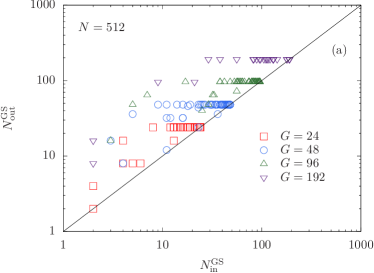
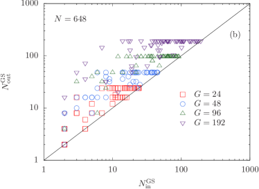
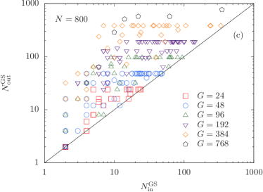
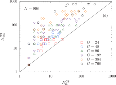
Figure 1: Number of solutions generated using cluster updates ($N^{\rm{GS}}_{\rm{out}}$) as a function of ground states found using the D-Wave 2X quantum annealer ($N^{\rm{GS}}_{\rm{in}}$) for different system sizes $N$ and known degeneracies $G$: (a) $N=512$, (b) $N=648$, (c) $N=800$, and (d) $N=968$. Each point represents an individual instance. Any points to the left of the $N^{\rm{GS}}_{\rm{out}}=N^{\rm{GS}}_{\rm{in}}$ (solid diagonal line) mean that additional minimizing configurations are found. For points that lie on the line, either all solutions were already known or the cluster updates produced no improvement.

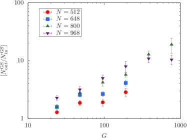
Figure 2: Relative improvement $[N^{\rm{GS}}_{\rm{out}}/N^{\rm{GS}}_{\rm{in}}]$ averaged over instances as a function of known degeneracy $G$ for different system sizes $N$ after postprocessing the minimizing configurations obtained with the D-Wave 2X quantum annealer. Square brackets represent a disorder average over all instances.

We now expand the data set produced by the D-Wave 2X quantum annealer in Ref. Mandrà et al. (2017) by including first-excited states in the resampling. When the algorithm is run, states that minimize the cost function are recorded while any other produced states are kept in the pool. This results in a clear advantage over the sampling of ground states: As mentioned, the cluster updates are not ergodic. This means that if the subset of minimizing configurations is small or from the same region in phase space, it will be hard for the algorithm to find other configurations in “more remote” parts of the phase space. However, by allowing first-excited states, this problem can be partially overcome. While some nonminimizing states are pushed into the ground-state manifold thus enriching the solution pool, some ground states are lifted out of the ground-state manifold into excited states to be pushed back at a later stage of the heuristic, however into a different part of phase space. For these experiments the cluster updates were applied $2^{17}$ times to each data set.

We note that the study can in principle be repeated for any number of low-lying states and does not need to be restricted to the first-excited state. In fact, the inclusion of higher-energy levels will allow the algorithm to more efficiently sample phase space.

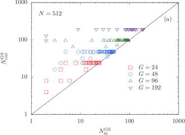
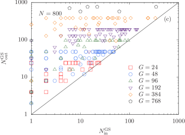
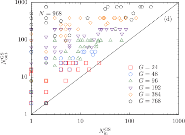
Figure 3: Number of solutions generated using cluster updates ($N^{\rm{GS}}_{\rm{out}}$) as a function of ground states found using the D-Wave 2X quantum annealer ($N^{\rm{GS}}_{\rm{in}}$) for different system sizes $N$ and known degeneracies $G$: (a) $N=512$, (b) $N=648$, (c) $N=800$, and (d) $N=968$. Each point represents an individual instance. Note that both ground states and first-excited states were fed into the cluster update in this experiment. Including a more diverse set of configurations and keeping track of minimizing configurations results in a better sampling of the ground-state manifold, as can be seen for cases where only one ground-state configuration was available and many more ground states were obtained by adding first excited states into the state pool (data points on the vertical axis).

Figure 3 shows scatter plots of individual instances produced using the D-Wave 2X quantum annealer for a given degeneracy $G$ and system size $N$. Here $N^{\rm{GS+ES}}_{\rm{in}}$ configurations (including first-excited states) are fed into the algorithm. The vertical axis represents the resulting ground-state configurations $N^{\rm{GS}}_{\rm{out}}$. The horizontal axis only depicts the ground-state configurations $N^{\rm{GS}}_{\rm{in}}$ fed into the cluster update for better comparison with the data in Fig. 1. Especially for large $G$ and $N$, the inclusion of excited states improves the sampling. Figure 4 goes to the extreme by only allowing nonminimizing first-excited states as input to the algorithm. As can be seen, the minimizing configurations can often be obtained from excited states alone. Only in a handful of cases (points on the horizontal axis) did the cluster updates not generate a minimizing configuration. This has an important consequence: Intrinsically bad data from a poor optimization technique can be postprocessed to find a minimizing configuration of the cost function, provided enough low-energy input states are available. We accomplish this by keeping track of the configurations with the lowest energy found.

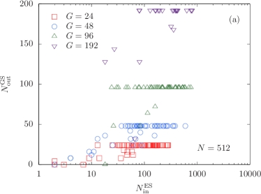
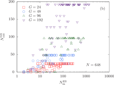
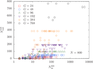
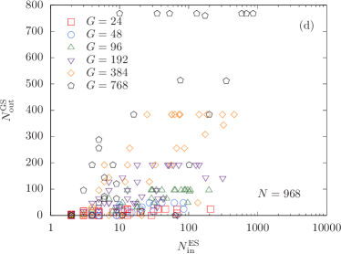
Figure 4: Number of solutions generated using cluster updates ($N^{\rm{GS}}_{\rm{out}}$) as a function of only excited states found using the D-Wave 2X quantum annealer ($N^{\rm{ES}}_{\rm{in}}$) for different system sizes $N$ and known degeneracies $G$: (a) $N=512$, (b) $N=648$, (c) $N=800$, and (d) $N=968$. Each point represents an individual instance. For all points that lie above the horizontal axis, the resampled excited states produced new minimizing configurations.

Next we attempt to systematically study the effects of a poor initial ground-state pool by restricting the initial set of minimizing configurations by a fraction $p$. In our experiments we use fractions of $25\%$ ($p=0.25$), $50\%$ ($p=0.50$), and $75\%$ ($p=0.75$). As done for the original data set (Table 1), we run the cluster updates $2^{20}$ times for each data set.

Figure 5 shows the relative improvement $\bm{[}[N^{\rm{GS}}_{\rm{out}}/(pN^{\rm{GS}}_{\rm{in}})]\bm{]}$ averaged over instances and ten independent subsets for different values of $p$ as a function of known degeneracy $G$ for different system sizes $N$ after postprocessing the minimizing configurations obtained with the D-Wave 2X quantum annealer. Note that the data are normalized by a factor $p$ such that when $\bm{[}[N^{\rm{GS}}_{\rm{out}}/(pN^{\rm{GS}}_{\rm{in}})]\bm{]}\to 1$ all known configurations are found. As can be seen, even when only $25\%$ of input states are used, all configurations can be found for large enough $G$. This shows that the method is asymptotically robust.

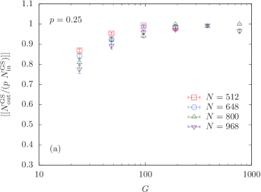
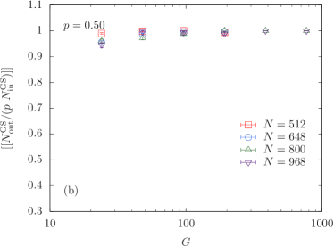
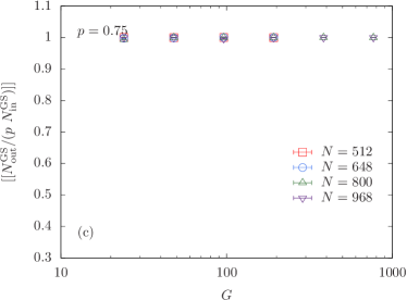
Figure 5: Relative improvement $\bm{[}[N^{\rm{GS}}_{\rm{out}}/(pN^{\rm{GS}}_{\rm{in}})]\bm{]}$ averaged over instances and ten independent runs as a function of known degeneracy $G$ for different system sizes $N$ and only using a fraction $p$ of available states after postprocessing the minimizing configurations obtained with the D-Wave 2X quantum annealer: (a) $p=0.25$, (b) $p=0.50$, and (c) $p=0.75$. The data are normalized such that for $\bm{[}[N^{\rm{GS}}_{\rm{out}}/(pN^{\rm{GS}}_{\rm{in}})]\bm{]}=1$ all known solutions in the initial ground-state pool are found. Double-square brackets $[[\ldots]]$ represent averages over instances and ten independent random trials.

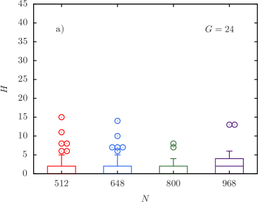
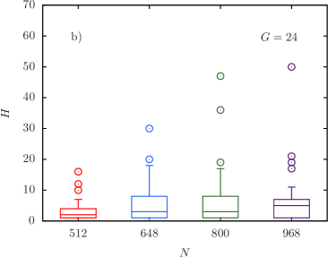
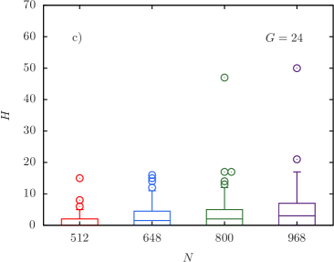
Figure 6: Maximum-minimum hamming distance versus the system size $N$ with degeneracy $G=24$ for the chimera graph. For each instance the minimum Hamming distance between each new ground state found and the original pool of configurations is calculated. The data shown are the maximum of these minima. The box represents the 25%-50% confidence interval, the center line is the median, the bars are the 5%-95% confidence interval, and the points are outliers. Data are shown from initial pools consisting of (a) only ground states, (b) only excited states, and (c) both ground states and excited states. Outliers represent non-trivial solutions with large Hamming distance from the initial pool found by the method.

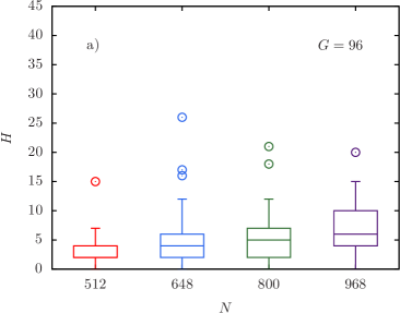
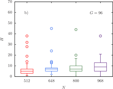
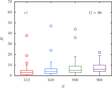
Figure 7: Maximum-minimum hamming distance versus the system size $N$ with degeneracy $G=96$ for the chimera graph. For each instance the minimum Hamming distance between each new ground state found and the original pool of configurations is calculated. The data shown are the maximum of these minima. The box represents the 25%-50% confidence interval, the centerline is the median, the bars are the 5%-95% confidence interval, and the points are outliers. Data are shownfrom initial pools consisting of (a) only ground states, (b) only excited states, and (c) both ground states and excited states. Outliers represent nontrivial solutions with large Hamming distance from the initial pool found by the method.

Finally, we illustrate the diversity of solutions found by the method. For each instance, we calculate the minimum Hamming distance of each new ground state from the pool of original ground states. From these minimum Hamming distances we take the maximum and analyze the maximum Hamming distance for each instance. This maximum-minimum Hamming distance $H$ shows if the method can find solutions which are not close in Hamming distance to the original pool.

Figures 6 and 7 show the maximum-minimum Hamming distance versus system size with degeneracy $G=24$ and $G=96$. The figures represent whether only ground states [Figs. 6(a) and 7(a)], only excited states [Figs. 6(b) and 7(b)], or both ground states and excited states [Figs. 6(c) and 7(c)] are included in the initial pool of states. The box represent the 25%-50% confidence interval, the centerline is the median, the bars are the 5%-95% confidence interval, and the points are outliers. Solutions found by the method are typically close to the original pool of solutions. In Figs. 6 and 7 the median increases with the system size to approximately $H=8$, which is consistent with the structure of the chimera Hamiltonian. Increasing the degeneracy from $G=24$ to $G=96$ also shows an improvement in the median Hamming distance. Nevertheless, there are many outliers that represent the diversity of solutions that would likely not be found with low-depth search starting from the initial pool of configurations, thus demonstrating the ability of the method to discover nontrivial solutions.

Summarizing, our results show that the resampling can overall improve ground-state data produced by the D-Wave 2X quantum annealer. However, these results can be applied more generally to any heuristic.

Table 2: Number of disorder instances $N_{\rm s}$ sorted by system size $N$ and number of ground states $G$ in three space dimensions. For each system size and ground-state degeneracy, the cluster update was applied $2^{20}$ times to the data set to produce new states for each study listed below com (c).

$N$	$G\!=\!8$	$G\!=\!12$	$G\!=\!16$	$G\!=\!20$	$G\!=\!24$	$G\!=\!32$	$N_{\rm s}$
$64$	$165$	$49$	$13$	$8$	$3$	$4$	$252$
$125$	$313$	$105$	$89$	$22$	$37$	$15$	$581$
$216$	$376$	$139$	$198$	$23$	$107$	$70$	$913$

III.3 Three-dimensional lattices

To study the effects of dimensionality, we now show experiments for three-dimensional cubic lattices. Our motivation lies in the fact that, in general, cluster updates become inefficient for dense graphs Zhu et al. (2015); Houdayer (2001). However, due to the intrinsic frustration of the problems, as well as the fact that we apply the updates at either zero or close-to-zero temperature, the cluster updates efficiently produce new states. Instances for $N=64$, $125$, and $216$ sites and couplers drawn from $J_{ij}\in\{\pm 5,\pm 6,\pm 7\}$ are initially optimized exactly using the spin-glass server jue . Note, however, that the spin-glass server only gives one minimizing configuration. To produce the data sets for resampling, we use simulated annealing Kirkpatrick et al. (1983) (Isakov et al. implementation Isakov et al. (2015) with $T_{\rm max}=10$, $T_{\rm min}=0.33$, $2^{14}$ sweeps, and $10^{5}$ repetitions for each sample). Instance parameters are listed in Table 2. Because the problems are relatively small, simulated annealing (even with a poor choice of parameters) tends to find all minimizing configurations. As such, we generated a synthetic data set where we only used first excited-states to verify that the cluster updates can use this information to find minimizing configurations.

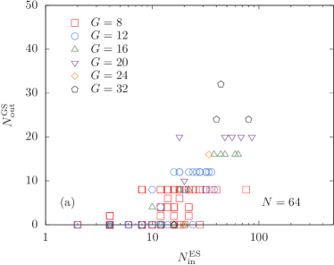
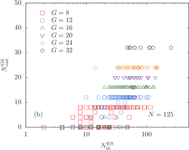
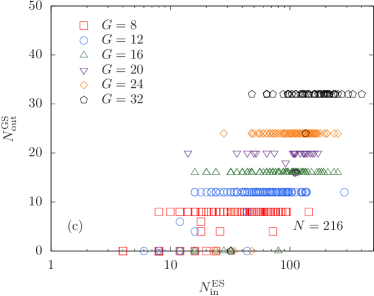
Figure 8: Number of solutions generated using cluster updates ($N^{\rm{GS}}_{\rm{out}}$) as a function of only excited states found using simulated annealing ($N^{\rm{ES}}_{\rm{in}}$) for different system sizes $N$ and known degeneracies $G$ for three-dimensional systems: (a) $N=64$ ($L=4$), (b) $N=125$ ($L=5$), and (c) $N=216$ ($L=6$). Each point represents an individual instance. For all points that lie above the horizontal axis, the resampled excited states produced new minimizing configurations. Note that for $N=64$ most instanced were solved, i.e., the pool of excited states is small.

Figure 8 shows results using only first-excited states as the input to the cluster updates in three space dimensions. As can be seen, minimizing configurations can be obtained from excited states only. This demonstrates that the cluster resampling works in space dimensions where, from a purely geometrical point of view, clusters would percolate and therefore be inefficient.

As done for the chimera topology in Sec. III.2, we use fractions of $25\%$ ($p=0.25$), $50\%$ ($p=0.50$), and $75\%$ ($p=0.75$) of the actual ground-state pool computed with simulated annealing. Figure 9 shows the relative improvement $\bm{[}[N^{\rm{GS}}_{\rm{out}}/(pN^{\rm{GS}}_{\rm{in}})]\bm{]}$ averaged over instances and ten independent subsets for different values of $p$ as a function of known degeneracy $G$ for different system sizes $N$ after postprocessing the minimizing configurations. Again, the data are normalized by a factor $p$ such that when $\bm{[}[N^{\rm{GS}}_{\rm{out}}/(pN^{\rm{GS}}_{\rm{in}})]\bm{]}\to 1$ all known configurations are found. As can be seen, even when only $25\%$ of input states are used, all configurations can be found for large enough $G$.

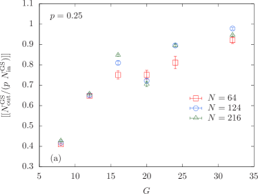
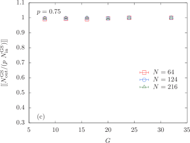
Figure 9: Relative improvement $\bm{[}[N^{\rm{GS}}_{\rm{out}}/(pN^{\rm{GS}}_{\rm{in}})]\bm{]}$ averaged over instances and ten independent runs as a function of known degeneracy $G$ for different system sizes $N$ and only using a fraction $p$ of available states after post-processing the minimizing configurations obtained with simulated annealing in three space dimensions. (a) $p=0.25$, (b) $p=0.50$, and (c) $p=0.75$. The data are normalized such that for $\bm{[}[N^{\rm{GS}}_{\rm{out}}/(pN^{\rm{GS}}_{\rm{in}})]\bm{]}=1$ all known solutions in the initial ground-state pool are found. Double-square brackets represent averages over instances and ten independent random trials.

III.4 Nondegenerate problems

Systems that have a unique ground state tend to be computationally more difficult than highly degenerate systems Katzgraber et al. (2015). In this section we study spin-glass Hamiltonians on the chimera lattice with couplers drawn from a Gaussian distribution with zero mean and unit standard deviation. These, by construction, have unique ground states. We generate a data set for different chimera lattice sizes with $N=8\times c^{2}$ variables using the D-Wave 2X quantum annealer. Because Gaussian couplers require high precision, the D-Wave analog annealer is notoriously bad at minimizing Gaussian problems. To illustrate how the cluster updates can improve low-quality data, in Fig. 10 we show histograms of the change in energy between the configurations produced by the D-Wave device and the same configurations after post processing them with the cluster updates. For each instance, $2^{17}$ resampling steps were performed of the approximately $100$ instances. As can be seen, the algorithm improves the data considerably and is (in some cases) able to find the actual ground-state configuration of the nondegenerate problem.

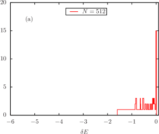
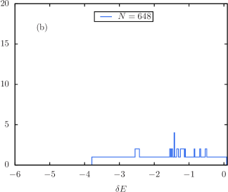
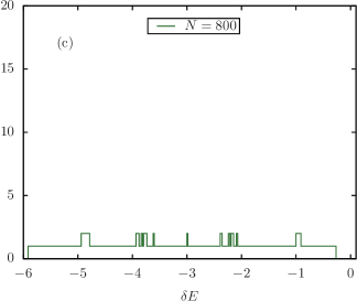
Figure 10: Histograms of the change in energy $\delta E$ between states found by the D-Wave 2X quantum annealer and the same states post processing them with the cluster updates for different system sizes $N=8\times c^{2}$ for problems with Gaussian-distributed couplers. (a) $N=512$, (b) $N=648$, and (c) $N=800$. In most cases lower-energy configurations were obtained using the cluster algorithm with the improvement becoming more pronounced for the larger system sizes.

We have also attempted to find the solutions to these instances using simulated annealing Isakov et al. (2015). Assuming that the obtained states are the true minimizing configurations, we study the fraction of solved problems as a function of system size for the D-Wave data, as well as the postprocessed data using the cluster algorithm. For example, for $N=483$ the fraction of problems solved increased from $0.58$ to $0.73$. Similarly, for $N=615$, the fraction of solved problems increased from $0.11$ to $0.29$. For smaller system sizes no noticeable improvement was observed, whereas for the largest problems with $758$ variables the cluster update found lower-energy configurations than simulated annealing was able to find.

III.5 Sampling at finite temperature

We now study the sampling of states at a finite temperature using the cluster updates. This is of importance for applications such as machine learning where a diverse pool of states is needed for the training step. For two replicas $(1)$ and $(2)$ needed for a cluster update the total energy $\Delta E^{(1)}+\Delta E^{(2)}=0$ has to be zero. However, the individual changes $\Delta E^{(1)}=-\Delta E^{(2)}$ can be nonzero. If these changes are typically small, then the cluster updates can be used to find uncorrelated samples at (best case) constant temperature.

For this study, we perform a full Monte Carlo simulation of a three-dimensional Ising spin glass using parallel tempering Monte Carlo Hukushima and Nemoto (1996) as well as isoenergetic cluster updates Zhu et al. (2015). System sizes of $N=4^{3}=64$, $5^{3}=125$, and $6^{3}=216$ are thermalized using $2^{18}$ Monte Carlo sweeps. For these small system sizes, the instances are thought to be equilibrated. Measurements are performed over an additional $2^{16}$ Monte Carlo sweeps. For the parallel tempering updates, $30$ temperatures in the range $[0.212,1.636]$ are used. However, in this case we are not interested in the thermal average of observables, except for the energy per spin $[\langle E\rangle]$ averaged both over disorder and Monte Carlo time. During the simulation, we keep track of the change in energy $\Delta E$ for each replica produced by a cluster update for a given sample and bin the data. Figure 11 shows histograms for $L=6$ of $\Delta E=|\Delta E^{(1)}|=|\Delta E^{(2)}|$ averaged over disorder. The horizontal axis has been shifted by the average energy per spin to better highlight the relative magnitude of the change. Both panels in the figure show the same data, with Fig. 11(b) using a vertical logarithmic scale to highlight the tails of the distribution. As can be seen, while there are pronounced tails, which corresponds to large changes in the energy of a given replica, the vast majority of changes in the energy are comparably small after a cluster update. Combining the cluster updates with a simple postprocessing where samples are only stored that have $\Delta E$ within a desired window, results in an efficient sampling of states at almost constant finite temperature.

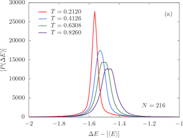
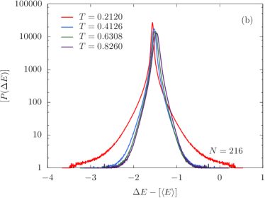
Figure 11: Histogram of the distribution of $\Delta E=|\Delta E^{(1)}|=|\Delta E^{(2)}|$ of cluster moves around the average thermodynamic energy $\langle E\rangle$ at different temperatures $T$ in three space dimensions ($N=216$) during a finite-temperature Monte Carlo simulation that includes cluster updates. In general, the changes in energy are small compared to the average energy with rare large rearrangements. Both panels show the same data set with (b) zooming into the tails.

III.6 Improvement of fair sampling on D-Wave quantum annealers

Reference Mandrà et al. (2017) demonstrated that transverse-field quantum annealing on the D-Wave 2X quantum annealer is not a fair sampling heuristic. In fact, because the problems studied have couplers in the range $J_{ij}\in\{\pm 5,\pm 6,\pm 7\}$, the energy gap between states is $\Delta E=2/7$. Thus one can perform detailed fair sampling statistics not only of the ground states, but also for excited states.

In order to better appreciate the exponential suppression of sampling on the D-Wave quantum device, it is possible to introduce the observable $\Theta_{\text{max}}$ defined as the maximum absolute difference of the empiric cumulative distribution $\tilde{F}(x)$ with respect to the cumulative of a uniform distribution $F(x)$, namely, $\Theta_{\text{max}}=\max_{x}|\tilde{F}(x)-F(x)|$, with $x$ the state index Mandrà et al. (2017). The test (which is similar in purpose to the Kolmogorov-Smirnov test) is useful to understand how close an empirical distribution is to the expected distribution. More precisely, the smaller $\Theta_{\text{max}}$ is, the more similar the distributions are. In general, the number of states at fixed energy $E$ that the D-Wave quantum annealer can find widely varies from instance to instance. To overcome this limitation, it is possible to compare the empiric $\Theta_{\text{max}}$ with a “baseline” computed by using an amount of uniformly distributed random numbers which is equal to the number of states with a given energy $E$ one was able to find Mandrà et al. (2017). This baseline plays an important role since it allows one to take into account finite-size effects that would erroneously give a false bias.

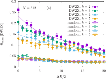
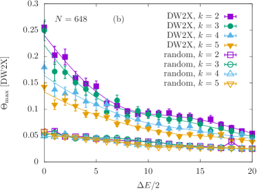
Figure 12: Comparison of $\Theta_{\text{max}}$ (maximum absolute difference of the empirical cumulative distribution with respect to the expected distribution, see the text) for the distribution of states found by the D-Wave 2X (DW2X) device at a given energy $E=E_{\text{gs}}+\Delta E$ for $N=512$ and $N=648$. The baseline for $\Theta_{\text{max}}$ is computed by using a random uniform distribution. As one can see, the bias in sampling for the D-Wave 2X device persists up to the $20^{\text{th}}$ level when $\Theta_{\text{max}}$ for the quantum annealer is comparable to the baseline.

Figure 12 shows the comparison of $\Theta_{\text{max}}$ for the distribution of states found by the D-Wave 2X device at a given energy $E=E_{\text{gs}}+\Delta E$, where $E_{\text{gs}}$ is the ground-state energy and $\Delta E$ are discrete (integer) energy shifts in multiples of $2/7$ above the ground state. As one can see, the bias not only is limited to the ground state, as reported in Ref. Mandrà et al. (2017), but is persistent up to the $20^{\text{th}}$ excited state.

We reanalyzed the data of Ref. Mandrà et al. (2017) using $2^{17}$ cluster updates. Figure 13 shows a side-by-side comparison of the data computed on the D-Wave device in Fig. 13(a) to the postprocessed data using the cluster updates in Fig. 13(b). Problems have been selected to have $G=3\times 2^{k}$ ground-state degeneracy. As can be seen clearly, the postprocessed data show less bias, i.e., the cluster updates can be applied to biased data sets to reduce biased sampling. By increasing the number of samples, the limiting distribution of uniform sampling follows ${\rm{erf}}^{-1}$ as shown in the Appendix.

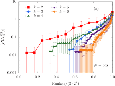
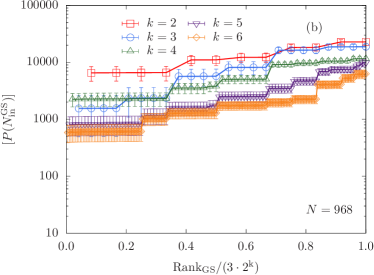
Figure 13: (a) Binned number of times a ground-state configuration is found using the D-Wave 2X quantum annealer sorted by rank compared to (b) the cluster-update post-processed data. Data for instances on a chimera lattice with $N$ sites and $G=3\times 2^{k}$ ground states are shown. The horizontal axis is normalized by $G$ for easier display of the data. While the magnitudes of the vertical axes are different in both panels, in both cases the range spans four orders of magnitudes. This allows for a direct visual comparison of the slopes. The raw data show a clear bias in (a) that is reduced considerably after applying the cluster updates shown in (b).

IV Summary and outlook

We have presented a cluster update routine that can vastly improve data sampling in polynomial time. The approach is based on isoenergetic cluster updates Zhu et al. (2015), first introduced for two-dimensional lattices by Houdayer Houdayer (2001). Using experimental data produced with the D-Wave 2X quantum annealer as well as synthetic data on a three-dimensional cubic lattice, we demonstrated different approaches to apply the cluster updates to improve sampling at both zero and finite temperatures. In particular, we demonstrated how the ground-state manifold of degenerate problems can be sampled more efficiently, as well as how finite-temperature data for, e.g., machine learning applications, can be used to produce more samples at either the same or similar temperature. We emphasize that the approach is generic and thus can be extended to many problems across disciplines. Application of resampling to machine learning and related applications is left to future work.

We recently became aware of the work in Ref. Dorband (2018). The approach is similar in nature to the work proposed here (also described in Refs. Ochoa (2017); Katzgraber et al. (2018)), however it only focuses on reducing the value of the cost function starting from a poor sample.

Appendix A Limit distribution for uniformly distributed random numbers

To understand the limit distribution of uniformly distributed random numbers, let us call $N$ the number of uniformly sampled random numbers among $M=3\times 2^{k}$ possible values (which correspond to the possible ground state configurations of a given instance). Since all the random numbers are uniformly sampled, the probability for a given value $m$ to have a number of hits $q$ is a binomial distribution of the form

$$P_{m}(q)=\binom{N}{q}p^{q}(1-p)^{N-q},$$ (2)

where $p=\frac{1}{M}$ is the probability that such a value is chosen every time a random number is extracted. In the limit of large $N$ and assuming that all the $P_{m}(q)$ are independent random variables, the histogram of the number of hits will follow a normal distribution with $\mu=\frac{N}{M}$ and variance $\sigma^{2}=\frac{N}{M}\left(1-\frac{1}{M}\right)\approx\frac{N}{M},$ that is, $q=\mathcal{N}(\mu,\sigma^{2})$. Therefore, after the reordering of the indices following the number of hits, the histogram should follow the inverse of the error function, that is,

$$q(x)=\sqrt{\frac{2N}{M}}\text{erf}^{-1}(2x-1)+\frac{N}{M},$$ (3)

where $x$ is the normalized index. Figures 14 and 15 compare the limit distribution of $N=10^{5}$ and $N=10^{6}$ random numbers uniformly sampled from $M=3\times 2^{k}$, with $k=5$, distinct values. As one can see, the empiric distribution is consistent with the limit distribution in Eq. (3). As expected, the slope of the normalized histogram is proportional to $\sqrt{\frac{1}{NM}}$ and it decreases by increasing the number of samplings $N$.

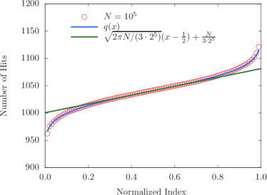
Figure 14: Number of hits for $N=10^{5}$ uniformly distributed random numbers among $3\times 2^{k}$ different values, with $k=5$. As expected, the histogram of number of hits follows the inverse of the error function.

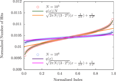
Figure 15: Normalized number of hits for $N=10^{5}$ and $N=10^{6}$ uniformly distributed random numbers among $3\times 2^{k}$ different values, with $k=5$. As shown in the figure, the normalized histogram becomes flatter by increasing the number of random numbers.