Small violations of Bell inequalities for multipartite pure random states

Abstract

For any finite number of parts, measurements and outcomes in a Bell scenario we estimate the probability of random $N$-qu$d$it pure states to substantially violate any Bell inequality with uniformly bounded coefficients. We prove that under some conditions on the local dimension the probability to find any significant amount of violation goes to zero exponentially fast as the number of parts goes to infinity. In addition, we also prove that if the number of parts is at least $3$, this probability also goes to zero as the the local Hilbert space dimension goes to infinity.

I Introduction

In his seminal paper Bell (1966), John Bell proved that, under certain assumptions, there exist predictions of quantum theory incompatible with those of any physical theory described by a Local Hidden Variable (LHV) Model Loubenets (2012, 2017); Brunner et al. (2014). Roughly speaking, these are models in which outcomes of spacelike separated measurements are independent conditionally on the knowledge of an underlying hidden variable. Bell’s key contribution was to show that LHV models must satisfy certain linear inequalities on joint probabilities that are now called Bell Inequalities, which quantum mechanics might violate. This is one of most important results in quantum physics Cabello (1996) so far, with deep implications to our knowledge of the world Vértesi and Brunner (2014); D. Rosset and Gisin (2014); Avis et al. (2009) and growing interest in practical applications Brunner et al. (2014); de Vicente (2014); Barrett et al. (2005). It is thus natural to ask how difficult it is to construct a quantum experimental setup that violates one of these inequalities Aspect (1975); Hensen et al. ; Hensen et al. (2016); Freedman and Clauser (1972); Winter (2014).

The present paper answers one variant of that question. Using probabilistic techniques González-Guillén et al. (2015, 2017); Palazuelos and Yin (2015); Palazuelos (2015); Loubenets (2012, 2017); Alon and Spencer ; Briët and Vidick (2013); Liang et al. (2010), and generalizing previous results of the authors in Drumond and Oliveira (2012), we are able to find an upper-bound for the typical behaviour of optimal violations for any Bell scenario $\Gamma=(N,m,v)$. We also discuss the effect of the size of the local dimension $d$ González-Guillén et al. (2015) on the probability that a $N$-partite $d$-dimensional quantum system violates any Bell inequality associated with this scenario. We find that , under some conditions, typical pure states do not produce large violations of Bell inequalities, in spite of the fact that they are likely to be highly entangled Brunner et al. (2014); Loubenets (2017). This apparent paradox sheds light on the important difference (not always made clear) between the concepts of entanglement Horodecki et al. (2009) and Bell non-locality Brunner et al. (2014).

The paper is organized as follows. Section II is devoted to set up some notation and definitions that will be used in the remainder of the paper. In Section III we discuss our main result, in the form of Theorem 1, and its consequences. In Section IV and Section V we give all key ingredients necessary to prove our main theorem. Section VI presents open questions, further works as well as our conclusions.

II Bell Inequalities

II.1 Basic Definitions

As our starting point in the paper, we consider multipartite device-independent, or black-box, scenarios Brunner et al. (2014); Pironio et al. (2016). That is, we consider a general correlation scenario, denoted by

$$\Gamma:=(N,m,v).$$ (1)

The triple $\Gamma$ describes a scenario with the following characteristics:

• $N$ black-boxes are distributed among $N$ players;

• each of these boxes admits $m$ different inputs; and

• for each input, among all $v$ possible distinct outputs, only one outcome is observed given that choice of input .

Without having direct access to all internal details of each box, the best description one has for $\Gamma$ is through the correlations among inputs and outputs. This means that such experimental scenarios should be described by a vector, $\vec{p}\in\mathds{R}^{(vm)^{N}}$ usually called behaviour Brunner et al. (2014); S. Tsirelson (1993). The components of such a vector are given by numbers

$$p_{a_{1},...,a_{N},x_{1},...,x_{N}}=P(a_{1},...,a_{N}|x_{1},...,x_{N}),$$ (2)

corresponding to the joint probability of obtaining the outcome list $(a_{1},...,a_{N})\in[v]\times...\times[v]$ given the inputs $(x_{1},...,x_{N})\in[m]\times...\times[m]$.

An admissible behaviour is a vector $\vec{p}\in\mathds{R}^{(mv)^{N}}$ that satisfies the following constraints:

$$P(a_{1},...,a_{N}|x_{1},...,x_{N})\in[0,1],\forall\,\,a_{1},...,a_{N},\forall\,\,x_{1},...,x_{N}$$ (3)

$$\sum_{a_{1},...,a_{N}}P(a_{1},...,a_{N}|x_{1},...,x_{N})=1,\,\,\forall\,\,x_{1},...,x_{m}.$$ (4)

We let $\mathcal{B}_{\Gamma}$ denote the set of all admissible behaviours associated with the correlation scenario $\Gamma=(N,m,v)$.

II.2 Non-Signalling and Local Hidden Variable Constraints

A behaviour $\vec{p}\in\mathcal{B}_{\Gamma}$ satisfies the non-signaling constraint when for all choices of subsets $\mathcal{I}\subset[N]$, say $\mathcal{I}=\{i_{1},...,i_{k}\}$, one has

$$\sum_{\begin{subarray}{c}a_{i}\\ i\in\mathcal{I}\end{subarray}}P(a_{1},...,a_{N}|x_{1},...,x_{N})=P(a_{i_{1}},...,a_{i_{k}}|x_{i_{1}},...,x_{i_{k}})=\sum_{\begin{subarray}{c}a_{i}\\ i\in\mathcal{I}\end{subarray}}P(a_{1},...,a_{N}|x_{1}^{\prime},...,x_{N}^{\prime}),\forall\,\,a_{i_{1}},...,a_{i_{k}}$$ (5)

for all possible inputs $(x_{1},...,x_{N})$ and $(x_{1}^{\prime},...,x_{N}^{\prime})$ with $x_{i_{1}}=x_{i_{1}}^{\prime}$, $\dots$, $x_{i_{k}}^{\prime}=x_{i_{k}}$. The set of all such behaviours is denoted by $\mathcal{NS}$.

We say that a behaviour $\vec{p}\in\mathds{R}^{(vm)^{N}}$ admits a local hidden variable (LHV) model when there exists a probability space $\mathcal{P}=(\Omega,\Sigma,\mu)$, and response functions

$$p(a_{i}|x_{i},\cdot):\Omega \longrightarrow[0,1]$$

$$\omega \mapsto p(a_{i}|x_{i},\omega)$$ (6)

such that, for every input and output one has  :

$$P(a_{1},...,a_{N}|x_{1},...,x_{N})=\int_{\Omega}p(a_{1}|x_{1},\omega)p(a_{2}|x_{2},\omega)...p(a_{N}|x_{N},\omega)\mu(d\omega).$$ (7)

The set of all behaviours $\vec{p}\in\mathcal{B}_{\Gamma}$ which admit a LHV model is called local set and denoted by $\mathcal{L}$. Notice that any admissible behaviour which admits a LHV model also satisfies the non-signalling constraints. In other words, the set of LHV models is contained inside the set of non-signalling behaviours.

In this paper we only consider scenarios in which the number of parts, the number of inputs and the number of outcomes are all finite. Therefore, we can assume Brunner et al. (2014) that the underlying probability space is also finite, and both $\mathcal{L}$ and $\mathcal{NS}$ are polytopes Schrijver (2003); Pitowsky (1991), the former with number of vertices $a=v^{mN}$ and affine dimension $D=(mv)^{N}$.

II.3 Bell Inequalities (with bounded coefficients)

A Bell inequality is defined through a linear functional $T$ acting on a behaviour $\vec{p}$:

$$T(\vec{p})=\sum_{\begin{subarray}{c}a_{1},...,a_{N}\\ x_{1},...,x_{N}\end{subarray}}T_{a_{1},...,a_{N}|x_{1},...,x_{N}}P(a_{1},...,a_{N}|x_{1},...,x_{N}),$$ (8)

where $T_{a_{1},...,a_{N}|x_{1},...,x_{N}}$ are real numbers. Defining $\Delta_{i}=\text{inf}_{\vec{p}\in\mathcal{L}}T(\vec{p})$ and $\Delta_{u}=\text{sup}_{\vec{p}\in\mathcal{L}}T(\vec{p})$, then

$$\sum_{\begin{subarray}{c}a_{1},...,a_{N}\\ x_{1},...,x_{N}\end{subarray}}T_{a_{1},...,a_{N}|x_{1},...,x_{N}}P(a_{1},...,a_{N}|x_{1},...,x_{N})\leq\Delta_{u},\text{ and }$$ (9)

$$\sum_{\begin{subarray}{c}a_{1},...,a_{N}\\ x_{1},...,x_{N}\end{subarray}}T_{a_{1},...,a_{N}|x_{1},...,x_{N}}P(a_{1},...,a_{N}|x_{1},...,x_{N})\geq\Delta_{i},$$ (10)

are tight Bell inequalities, in the sense that they are satisfied by all local behaviours and, in addition, there exists at least one local behaviour saturating each bound. For the sake of simplicity in defining the degree of violation of such inequalities (see Eq. 24 below), but without loss of generality, we assume throughout the paper that

$$\text{max}\{|\Delta_{i}|,|\Delta_{u}|\}=1.$$ (11)

We denote the set of all linear functionals defining Bell inequalities (for a fixed scenario) by $\mathcal{T}$. For any $b>0$, we denote by $\mathcal{T}_{b}$ the subset of $\mathcal{T}$ where all coefficients (components of the linear functional) are bounded by $b$, that is

$$\mathcal{T}_{b}=\{T\in\mathcal{T}:|T_{a_{1},...,a_{N}|x_{1},...,x_{N}}|\leq b\text{ for all }a_{1},...,a_{N},x_{1},...,x_{N}\}.$$ (12)

One the one hand, whatever the value that $b$ assumes, $\mathcal{T}_{b}$ will always be a proper subset of $\mathcal{T}$. Indeed, due to the constraints satisfied by the components of behaviours, one can insert terms with arbitrarily large coefficients to the functional (8) without ever altering its value on behaviours.

On the other hand, as we will argue below, using again these same constraints, one can show that every Bell inequality (9) and (10) defined by a functional is equivalent  to one whose functional only has non-negative coefficients and belongs to $\mathcal{T}_{1}$. This possibility is often tacitly assumed Cabello et al. (2010, 2014); Rafael et al. (2014); Collins et al. (2002); López-Rosa et al. (2016); Śliwa (2003) and many notable inequalities are of this kind. For instance, all three Sadiq et al. (2013) pentagonal Bell inequalities

$$I^{P}_{1} =P(00|00)+P(11|01)+P(10|11)+P(00|10)+P(11|00)\leq 2;$$ (13)

$$I^{P}_{2} =P(00|00)+P(11|01)+P(10|11)+P(00|10)+P(\_1|\_0)\leq 2;$$ (14)

$$I^{P}_{3} =P(00|00)+P(11|01)+P(10|11)+P(00|10)+P(11|20)\leq 2$$ (15)

as well as a symmetric version of the simplest tight Bell inequality (after CHSH) violated by quantum theory Froissart (1981); Collins and Gisin (2004); Brunner and Gisin (2008):

$$I_{3322}= P(00|01)+P(00|02)+P(00|10)+P(00|12)+P(00|20)+P(00|21)$$ (16)

$$+P(01|11)+P(10|11)+P(11|11)+P(01|22)+P(10|22)+P(11|22)$$ (17)

$$+P(1\_|0\_)+P(1\_|1\_)+P(\_1|\_0)+P(\_1|\_1)\leq 6,$$ (18)

are examples of it (upon normalizing the classical bound).

In addition, recently the authors in Cabello et al. (2010, 2014); Rafael et al. (2014) have made a heavy use of the fact that any Bell inequality can be rewritten as an equivalent inequality with positive coefficients lying in $\mathcal{T}_{b}$, with $b>0$. Starting from a Bell inequality with positive coefficients they associate a graph $\mathcal{G}$ representing that inequality. Each event is associated with a vertex, and two vertices are connected whenever their underlying events are exclusive Rafael et al. (2014). The weight of each vertex in that representation being given by the positive coefficient associated with the underlying event in the Bell inequality. Having constructed such a weighted-graph, the authors have shown that $i)$ the classical bounded for the original inequality is given by $\alpha(\mathcal{G})$ the independence number of $\mathcal{G}$, that $ii)$ the maximal quantum violation is $\vartheta(\mathcal{G})$ the Lovász number of $\mathcal{G}$, and that $iii)$ the maximum value admissible for more general probabilistic theories is $\alpha^{\ast}(\mathcal{G})$ the fractional-packing number of $\mathcal{G}$. It shows that such rewritings are not only aesthetic tricks, they do have provided fruitful results for the analysis of violations of Bell inequalities.

Indeed, suppose we are given a Bell inequality (9) and assume $\Delta_{u}>0$. If

$$\mathcal{I}=\{(a_{1},...,a_{N},x_{1},...,x_{N})\in[v]^{N}\times[m]^{N}:\,\,T_{a_{1},...,a_{N}|x_{1},...,x_{N}}<0\},$$ (19)

for each element $(a_{1}^{\prime},...,a_{N}^{\prime},x_{1}^{\prime},...,x_{N}^{\prime})\in\mathcal{I}$ we can use the fact that probabilities are normalized to write

$$P(a_{1}^{\prime},...,a_{N}^{\prime}|x_{1},...,x_{N})=1\,\,\,-\sum_{a_{1}\neq a_{1}^{\prime},...,a_{N}\neq a_{N}^{\prime}}P(a_{1},...,a_{N}|x_{1},...,x_{N}),$$ (20)

and change all terms with negative coefficients appearing in Eq. (9) by a sum of terms with positive coefficients plus some negative constants. Leaving all terms with probabilities on the l.h.s of the inequality and all constants on the r.h.s, the new inequality has classical bound $\Theta=\Delta_{u}-\sum_{(a_{1},...,a_{N}|x_{1},...,x_{N})\in\mathcal{I}}T_{a_{1},...,a_{N}|x_{1},...,x_{N}}>0$. Dividing both sides by $\Theta$, we obtain an inequality

$$\sum_{\begin{subarray}{c}a_{1},...,a_{N}\\ x_{1},...,x_{N}\end{subarray}}\tilde{T}_{a_{1},...,a_{N}|x_{1},...,x_{N}}P(a_{1},...,a_{N}|x_{1},...,x_{N})\leq 1,$$ (21)

whose coefficients are non-negative and, therefore, bounded by $1$ (otherwise it would be possible to construct a LHV theory violating the inequality). A similar trick can be done if $\Delta_{u}<0$ and to inequality (10).

II.4 Degree of violations by quantum states

A test of a Bell inequality (9) or (10) can be designed for a quantum system by choosing $m$ POVM’s with $v$ outcomes, $\{\Pi_{a_{k},x_{k}}^{k}\}_{a_{k}=1}^{v}$, for each part $k$. We denote by $A$ the collection of these POVM’s and define the so-called Bell operator

$$\mathfrak{B}_{T,A}:=\sum_{\begin{subarray}{c}a_{1},...,a_{N}\\ x_{1},...,x_{N}\end{subarray}}T_{a_{1},...,a_{N}|x_{1},...,x_{N}}\Pi_{a_{1},x_{1}}^{1}\otimes...\otimes\Pi_{a_{N},x_{N}}^{N}.$$ (22)

Moreover, we denote by $\mathcal{A}$ the set of all possible POVM’s choices for a fixed scenario and $N$-fold tensor product of Hilbert spaces. A (possible) violation for the Bell inequality is then evaluated through the function:

$$Q(\ket{\psi},T,A)=\text{Tr}(\mathfrak{B}_{T,A}\left|\psi\rangle\!\langle\psi\right|).$$ (23)

Whenever $|Q(\ket{\psi},T,A)|>1$ one of Bell inequalities with coefficients $T$ is violated by the local measurements described by $A$. For that reason, it makes sense that the degree of violation Loubenets (2012, 2017); Palazuelos and Yin (2015); Palazuelos (2015) should be defined by the quantity

$$|Q(\ket{\psi},T,A)|.$$ (24)

It will be crucial for our results the bounds on quantum violations of Bell inequalities found by Loubenets in Loubenets (2017), which guarantees that

$$|Q(\ket{\psi},T,A)|\leq(2m-1)^{N}$$ (25)

for all $T$ and $A$ associated with a fixed scenario, and all $\ket{\psi}$ of any $N$-fold tensor product Hilbert space.

III Small Probabilities of High Violations

It is already known Brunner et al. (2014); Loubenets (2017); Palazuelos (2015) that if either the local dimension $d$ of each quantum system, or the number $N$ of parts, is sufficiently large, then typical quantum states are highly entangled. Should we expect, then, that typically there will be at least one Bell inequality that is greatly violated? Our main objective in the present work is, then, to approach the following question:

given a typical pure state $\ket{\psi}$ composed by $N$ $d-$dimensional quantum systems, what should one expect for its largest possible violation over all relevant Bell inequalities in a given scenario $\Gamma=(N,m,v)$?

In our framework, optimal violations (if any) of Bell inequalities exhibited by a quantum state $\ket{\psi}\in(\mathds{C}^{d})^{\otimes N}$ are given by the functional (see Eq. (23)):

$$V_{\text{opt}}(\ket{\psi}):=\sup_{\begin{subarray}{c}A\in\mathcal{A}\\ T\in\mathcal{T}_{b}\end{subarray}}|Q(\ket{\psi},T,A)|,$$ (26)

where the supremum is taken over all quantum implementations of all Bell inequalities whose coefficients are uniformly bounded by $b$.

Remark: Our restriction to optimize the violations over $\mathcal{T}_{b}$ has basically a technical motivation: we need to assume it in order to successfully apply our techniques. On the one hand, as we have pointed out in Sec II.3, it holds that for any fixed $b>1$, every possible Bell inequality is equivalent to one obtained by a functional in $\mathcal{T}_{b}$. At first sight this fact apparently makes irrelevant our restriction. On the other hand, for a fixed quantum state, its optimal degree of violation may be different even for two equivalent Bell inequalities (as one can test on simple examples). We do not know, for instance, how to rule out the existence of a family of pure quantum states for $N$ parties whose optimal violations only takes place on Bell inequalities whose coefficients becomes arbitrary large with $N$. The fact is we are not sure of such a restriction to bounded coefficients is relevant or not. However, even if it is, we recall from the discussion in section II.3 that we still would be able to encompass a huge class of relevant Bell inequalities.

Now, if $\ket{\psi}$ is a point of a sample space, since $V_{\text{opt}}$ is a function of $\ket{\psi}$ we can consider it as a random variable. Formally, what we would like to estimate is the distribution function of such variable, that is:

$$\mathds{P}(V_{\text{opt}}>c).$$ (27)

It is known Popescu and Rohrlich (1992); Cavalcanti et al. (2011) that any entangled $N$-partite pure state violate some Bell inequality. Since these states have full measure on the sphere of pure states, its is clear then that $\mathds{P}(V_{\text{opt}}>c)=1$ for $c\leq 1$. For arbitrary $c>1$ we have our main result:

Theorem 1.

Given $N,d\geq 2$ integers. Let $\ket{\psi}\in\left(\mathds{C}^{d}\right)^{\otimes N}$ be a unit vector distributed according to the uniform measure in the sphere $S_{2d^{N}-1}$ of $\left(\mathds{C}^{d}\right)^{\otimes N}$, then:

$$\mathds{P}(V_{\text{\emph{opt}}}>c)\leq 4\left[\frac{8bN(mv)^{N}d^{2}}{\delta}+2\right]^{mvNd^{2}+(mv)^{N}}\times e^{-\left(\frac{2d^{N}(c-\delta-1)^{2}}{36\pi^{2}(2m-1)^{2N-2}}\right)},$$ (28)

for any $b,\delta>0,\,\,c>\delta+1$.

This theorem allows us to answer the question posed at the beginning of this section negatively. A typical state $\ket{\psi}$ composed by $N$ $d$-dimensional quantum systems, with $N$ and/or $d$ large enough, does not exhibit a significant degree of violation for any Bell inequality (with uniformly bounded coefficients).

In fact, note that it is possible to rewrite Eq. 28 as follows (see Appendix A):

$$\mathds{P}(V_{\text{opt}}>c)\leq 4\exp\left\{mvN^{2}d^{2}\log(mv)+mvNd^{2}\log\left(\frac{16bNd^{2}}{\delta}\right)\right.+ (mv)^{N}\log\left(\frac{16Nd^{2}}{\delta}\right)+N(mv)^{N}\log(bmv)$$

$$\left.-\frac{(c-\delta-1)^{2}(2m-1)^{2}}{18\pi^{2}}\left[\frac{d}{(2m-1)^{2}}\right]^{N}\right\}.$$ (29)

Now, on the one hand, if the local dimension $d$ of each subsystem satisfies

$$d>mv(2m-1)^{2},$$ (30)

and if in addition the uniform bound $b$ is not too large, e.g. if

$$b=\mathcal{O}\left((mn)^{N}\right),$$ (31)

then the fifth term in brackets dominates all other terms. So, we are left with:

$$\mathds{P}(V_{\text{opt}}>c)\rightarrow 0$$ (32)

super-exponentially fast as $N\rightarrow\infty$. Consequently:

if the local dimension $d$ of a $N$-partite quantum system satisfies $d>mv(2m-1)^{2}$, then, for large $N$, the vast majority of pure states will not violate any Bell inequality with bounded coefficients to any significant degree.

On the other hand, assume that $N\geq 3$ and that all parameters, except $d$ are fixed. Hence, as $d$ becomes arbitrarily large, we also see from Eq. (29) that the probability of finding a violation goes to zero. Putting into words:

for any $N\geq 3$, if the local dimension $d$ is large enough, the vast majority of pure states will not violate any Bell inequality with bounded coefficients to any significant degree.

To sum up, we can formally state:

Corollary 2.

Let $\ket{\psi}\in\left(\mathds{C}^{d}\right)^{N}$ be a unit vector distributed according to the uniform measure in the sphere $S_{2d^{N}-1}$ of $\left(\mathds{C}^{d}\right)^{N}$. Given integers $N\geq 2$ and $d\geq 2$, and given $b>0$ the following statements below hold true:

• If $d$ the local dimension satisfies $d>vm(2m-1)^{2}$, then

  $$\mathds{P}(V_{\text{{opt}}}>c)\rightarrow 0,\,\,\,\mbox{as}\,\,\,N\rightarrow\infty.$$ (33)

• If $N$ the number of parts satisfies $N\geq 3$, then:

  $$\mathds{P}(V_{\text{{opt}}}>c)\rightarrow 0,\,\,\mbox{as}\,\,\,d\rightarrow\infty.$$ (34)

So, in spite the fact that typically any $N$-partite pure state, with large $N$ and/or $d$, is highly entangled, the typical value of the Bell violation is extraordinarily small.

IV The Proof

IV.1 Idea of the proof

We first decompose the event $\{V_{\text{{opt}}}>c\}$ into a union of pieces corresponding to each possible choice of POVM’s and Bell inequality coefficients, as well as in violations from above and violations from below. This gives:

$$\mathds{P}\left(\ket{\psi}:\sup_{\begin{subarray}{c}A\in\mathcal{A}\\ T\in\mathcal{T}_{b}\end{subarray}}|Q(\ket{\psi},T,A)|>c\right) =\mathds{P}\left(\left[\bigcup_{\begin{subarray}{c}A\in\mathcal{A}\\ T\in\mathcal{T}_{b}\end{subarray}}\{\ket{\psi}:Q(\ket{\psi},T,A)>c\}\right]\bigcup\left[\bigcup_{\begin{subarray}{c}A\in\mathcal{A}\\ T\in\mathcal{T}_{b}\end{subarray}}\{\ket{\psi}:Q(\ket{\psi},T,A)<-c\}\right]\right)$$ (35)

$$=2\mathds{P}\left(\bigcup_{\begin{subarray}{c}A\in\mathcal{A}\\ T\in\mathcal{T}_{b}\end{subarray}}\{\ket{\psi}:Q(\ket{\psi},T,A)>c\}\right).$$ (36)

The first equality comes from the fact that the events considered are the same. In the disjoint in the r.h.s of Eq. (35), the fact that $Q$ is linear in $T$ guarantees that the two events have equal measure, which gives the second equality. Even though the event appearing on (36) is given by an infinite union of sets, the strategy is to replace it by a finite union without, however, changing too much its probability. This replacement is done trough suitable $\epsilon$-nets for $\mathcal{A}$ and $\mathcal{T}$. We then just apply the union bound, together with a uniform bound on the probability distribution for the degree of violation for any fixed inequality with functional $T$ and measurement settings $A$. This strategy results in the bound of Theorem 1 which has two terms as distinguished below:

$$\mathds{P}(V_{\text{{opt}}}>c)\leq 4\underbrace{\left[\frac{8bNd^{2}(mv)^{N}}{\delta}+2\right]^{mvNd^{2}}}_{(A)}\times\underbrace{\text{exp}{\left(-\frac{2d^{N}(c-\delta-1)^{2}}{36\pi^{2}(2m-1)^{2N-2}}\right)}}_{(B)},$$ (37)

The term $(A)$ in Eq. (37) is just an estimate of the number of points of the $\epsilon-$net. Term $(B)$ is the uniform bound mentioned above. It results basically from Lévy’s lemma Ledoux (2001) together with a pair of results on the smoothness of the $Q$ function.

IV.2 Some lemmas

Note that $Q(\ket{\psi},A,T)$ is a function of three variables: $i)$ $\ket{\psi}$, belonging to a sample space, $ii)$ $A\in\mathcal{A}$, which can be conveniently seen as an element of a metric space, as we are going to discuss later on subsequent subsections, and $iii)$ $T\in\mathcal{T}$ also belonging to a suitable metric set.

The first step is show the possibility of replacing the infinite sets $\mathcal{A}$ and $\mathcal{T}$ by finite “representative” subsets of them, without changing much the optimal violation. This can be made precise by the following lemma.

Lemma 3.

Let $\varphi:\Omega\times M\rightarrow\mathds{R}$ be such that $\Omega$ is a sample space and $M$ a metric space. For a given $\delta>0$, suppose that there exists a finite $M_{\delta}^{\prime}\subseteq M$ such that for every $x\in M$ there is $x^{\prime}\in M_{\delta}^{\prime}$ where $|\varphi(\omega,x)-\varphi(\omega,x^{\prime})|<\delta$ for every $\omega\in\Omega$. Then, for every $c>0$, with $c-\delta>0$, we have

$$\mathds{P}\left(\omega:\sup_{x\in M}\{\varphi(\omega,x)\}>c\right)\leq\sum_{x^{\prime}\in M_{\delta}^{\prime}}\mathds{P}\left(\omega:\varphi(\omega,x^{\prime})>c-\delta\right).$$ (38)

Proof.

Take $\omega_{*}\in\Omega$ such that $\sup_{x\in M}\{\varphi(\omega_{*},x)\}>c$. There exists then a $x\in M$ with $\varphi(\omega_{*},x)>c$. Replacing $x$ by some $x^{\prime}\in M^{\prime}_{\delta}$ with $|\varphi(\omega_{*},x)-\varphi(\omega_{*},x^{\prime})|<\delta$, we obtain $\varphi(\omega_{*},x^{\prime})>c-\delta$. Therefore, we have the following set inclusion.

$$\{\omega:\sup_{x\in M}\{\varphi(\omega,x)\}>c\}\subseteq\bigcup_{x^{\prime}\in M_{\delta}^{\prime}}\{\omega:\varphi(\omega,x^{\prime})>c-\delta\}.$$ (39)

The lemma now follows from a union bound on the set on the right hand side of the inclusion. 

For our problem we will construct such a finite set based on an $\epsilon$-net Haussler and Welzl (1987); Briët and Vidick (2013) of a hypercube. Letting $||x||_{\infty}=\text{max}_{i=1,..n}|x_{i}|$, for $x=(x_{1},...,x_{n})\in\mathds{R}^{n}$, we can state the following:

Lemma 4.

Given $n\in\mathds{N}$, a subset $X$ of $[-1,1]^{n}$ and $0<\epsilon<1$, there exists a finite subset $N_{\epsilon}\subset X$ such that for every $x\in X$ there exists $x^{\prime}\in N_{\epsilon}$ with $||x-x^{\prime}||_{\infty}<\epsilon.$ Moreover,

$$|N_{\epsilon}|<\left(\frac{2}{\epsilon}+2\right)^{n}.$$ (40)

Proof.

Let $l=\lceil 1/\epsilon\rceil$ be the smallest integer greater than $1/\epsilon$. We can see the whole hypercube as the union of small hypercubes

$$h_{j_{1},...,j_{n}}=\prod_{k=1}^{n}\left[\frac{j_{k}}{l},\frac{j_{k}+1}{l}\right],$$ (41)

where $j_{k}\in\{-l,-l+1,...,-1,0,1,2,...,l-1\}$. Note that their edges have length $1/l$, so two points $a,b$ inside them satisfy $||a-b||_{\infty}\leq 1/l=1/\lceil 1/\epsilon\rceil\leq\epsilon$. Whenever $X\bigcap h_{j_{1},...,j_{n}}\neq\emptyset$ take a single point $x_{j_{1},...,j_{n}}$ of $X$ in that intersection, and let $N_{\epsilon}$ be the collection of such points. It is indeed finite and its number is at most the total number of small hypercubes, $|N_{\epsilon}|\leq(2l)^{n}<(2/\epsilon+2)^{n}.$ Take now arbitrary $x\in X$. Since $X\subseteq[-1,1]^{n}$, $x$ belongs to some small hypercube $h_{j_{1}^{\prime},...,j_{n}^{\prime}}$, for some choice of indexes $\{j_{1}^{\prime},...,j_{n}^{\prime}\}$. If we take the single $x_{j_{1}^{\prime},...,j_{n}^{\prime}}\in N_{\epsilon}$ in that hypercube, we have $||x-x_{j_{1}^{\prime},...,j_{n}^{\prime}}||\leq\epsilon$, since both $x$ and $x_{j_{1}^{\prime},...,j_{n}^{\prime}}$ belongs to $h_{j_{1}^{\prime},...,j_{n}^{\prime}}$.  

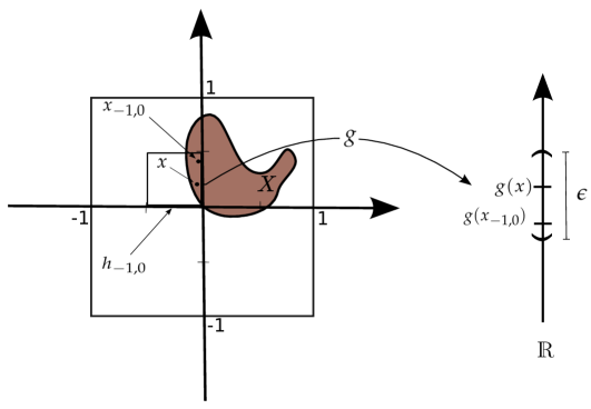
Figure 1: Schematic drawing of $X\subset[-1,1]^{2},$ and a small hypercube $h_{-1,0}$ intersecting it with $\epsilon=\frac{1}{2}$. Here we are showing an arbitrary choice of a point $x_{-1,0}\in N_{\epsilon}$, given $x\in X$, such that $|g(x)-g(x_{-1,0})|<\epsilon$ (colours online).

With Lemma 4 in our hands, we have immediately (see Fig. 1):

Corollary 5.

Suppose that for $g:X\rightarrow\mathds{R}$, where $X\subseteq[-1,1]^{n}$, there exists $\lambda>0$ such that $|g(x)-g(x^{\prime})|\leq\lambda||x-x^{\prime}||_{\infty}$ for all $x,x^{\prime}\in X$. Given $\delta>0$ there exists a set $N_{\delta/\lambda}\subset X$ with number of elements bounded by $(2\lambda/\delta+2)^{n}$ such that for every $x\in X$, there is $x^{\prime}\in N_{\delta/\lambda}$ with $|g(x)-g(x^{\prime})|<\delta$.

Finally, we shall use Lévy’s Lemma (see Ledoux (2001)):

Lemma 6.

For every $\epsilon>0$, $D\geq 1$ integer and $F:S_{D}\rightarrow\mathds{R}$ a real-valued function with Lipschitz constant $\Lambda$ (w.r.t the Euclidean distance), the following inequality holds true:

$$\mathds{P}(F-\mathds{E}[F]>\epsilon)\leq 2e^{-\frac{(D+1)\epsilon^{2}}{9\pi^{3}\Lambda^{2}}},$$ (42)

where $\mathds{P}$ denotes the uniform probability measure on the $D-$dimensional unity sphere $S_{D}$.

V Putting all together

Now, take a function $\varphi$ as in Lemma 3. Assume that $M=[-1,1]^{n}$ and there exists a $\lambda>0$ such that $|\varphi(\omega,x)-\varphi(\omega,x^{\prime})|\leq\lambda||x-x^{\prime}||_{\infty}$ for all $\omega\in\Omega$ and $x,x^{\prime}\in[-1,1]^{n}$. Given $c>\delta>0$, we can use Lemma 3 and Corollary 5 to show that:

$$\mathds{P}\left(\omega:\sup_{x\in[-1,1]^{n}}\{\varphi(\omega,x)\}>c\right)\leq(2\lambda/\delta+2)^{n}\max_{x^{\prime}\in N_{\lambda/\delta}}\mathds{P}\left(\omega:\varphi(\omega,x^{\prime})>c-\delta\right).$$ (43)

Let us assume additionally that $\Omega=S_{D}$ for some $D\in\mathds{N}$, that $\mathds{E}[\varphi(\cdot,x)]\leq 1$ for all $x\in M$, and that there exists non-negative $\Lambda\in\mathds{R}$ such that

$$|\varphi(\omega,x)-\varphi(\omega^{\prime},x)|\leq\Lambda|\omega-\omega^{\prime}|,\,\,\mbox{for all}\,\,x\in[-1,1]^{n},\omega,\omega^{\prime}\in S_{D},$$ (44)

with $|\omega-\omega^{\prime}|$ being the Euclidean distance on the sphere. That is, $\varphi$ is Lipschitz with with respect to $\omega$, with Lipschitz constant $\Lambda$ independent of $x$. These assumptions allow us to apply Lévy’s Lemma, and bound the probability appearing on the r.h.s of Equation (43) in order to get, for all $c>\delta+1$, the bound:

$$\mathds{P}\left(\omega:\sup_{x\in[-1,1]^{n}}\{\varphi(\omega,x)\}>c\right)\leq 2(2\lambda/\delta+2)^{n}e^{-\frac{(D+1)(c-\delta-1)^{2}}{9\pi^{3}\Lambda^{2}}}.$$ (45)

We now come back to the setting of Theorem 1. We apply (45) to the events in Eq. (36). We set $\varphi=Q$, $\omega=\ket{\psi}$ and $x=(T,A)$, that is, $M=\mathcal{T}\times\mathcal{A}$. The set of pure states $\ket{\psi}$ is a sphere $S_{D}$ with $D=2d^{N}-1$. Moreover, an upper bound for the mean value of $Q$ follows straightforwardly from the fact that the expectation $\mathds{E}[Q(\ket{\psi},T,A)]$ corresponds to replacing $\ket{\psi}$ with the maximally mixed state, with which the Bell inequality is certainly satisfied:

$$\mathds{E}[Q(\ket{\psi},T,A)]\leq 1.$$ (46)

In order to apply our tools, we will parametrize $\mathcal{T}\times\mathcal{A}$ by a subset of $[-1,1]^{n}$, for some $n$, and find $\lambda$ and $\Lambda$ as described above. We will then obtain the bound:

$$\mathds{P}\left[\ket{\psi}:\sup_{\begin{subarray}{c}A\in\mathcal{A}\\ T\in\mathcal{T}\end{subarray}}Q(\ket{\psi},T,A)>c\right]\leq 4(2\lambda/\delta+2)^{n}e^{-\frac{(2d^{N})(c-\delta-1)^{2}}{9\pi^{3}\Lambda^{2}}}.$$ (47)

In the following subsections we $i)$ show the existence, and $ii)$ obtain an estimative for the values of $n,\lambda,\Lambda$, which, inserted on the above expression, provides the proof of Theorem 1.

V.1 Bounding the Lipschitz constant of $Q$ (estimating $\Lambda$)

In order to show that the functional $Q$ is Lipschitz with respect to $\ket{\psi}$, firstly note that:

$$\forall\ket{\psi},\ket{\psi^{\prime}}:|Q(\ket{\psi},T,A)-Q(\ket{\psi^{\prime}},T,A)| =|\bra{\psi}\mathcal{B}_{T,A}\ket{\psi}-\bra{\psi^{\prime}}\mathcal{B}_{T,A}\ket{\psi^{\prime}}|$$ (48a)

$$=\left|\text{Tr}\left[\left(\sum_{\begin{subarray}{c}j_{1},...,j_{N}\\ o_{1},...o_{N}\end{subarray}}T_{\begin{subarray}{c}j_{1},...,j_{N}\\ o_{1},...o_{N}\end{subarray}}\bigotimes_{i=1}^{N}\Pi_{j_{i},o_{i}}^{i}\right)(\ket{\psi}\bra{\psi}-\ket{\psi^{\prime}}\bra{\psi^{\prime}})\right]\right|$$ (48b)

$$\leq\left\|\sum_{\begin{subarray}{c}j_{1},...,j_{N}\\ o_{1},...o_{N}\end{subarray}}T_{\begin{subarray}{c}j_{1},...,j_{N}\\ o_{1},...o_{N}\end{subarray}}\bigotimes_{i=1}^{N}\Pi_{j_{i},o_{i}}^{i}\right\|\left\|\ket{\psi}\bra{\psi}-\ket{\psi^{\prime}}\bra{\psi^{\prime}}\right\|_{1}$$ (48c)

$$=\left\|\mathcal{B}_{T,A}\right\|\left\|\ket{\psi}\bra{\psi}-\ket{\psi^{\prime}}\bra{\psi^{\prime}}\right\|_{1}$$ (48d)

$$\leq 2(2m-1)^{N-1}\left\|\ket{\psi}-\ket{\psi^{\prime}}\right\|_{2}.$$ (48e)

Here $\|\mathcal{B}_{T,A}\|$ stands for the usual operator norm, and (48c) follows from von Neumann’s trace inequality Mirsky (1975) plus Hölder’s inequality. The bound for the Bell operator in (48e) follows from the fact that it is self-adjoint and Eq. (25). Therefore, a Lipschitz constant for $Q$ is

$$\Lambda=2(2m-1)^{N-1}.$$ (49)

V.2 Variation of $Q$ with $\mathcal{A}$ and $\mathcal{T}$ (finding $n$ and $\lambda$)

V.2.1 Variation of $Q$ with measurements $A$

Now we proceed to estimate how the function $Q(\psi,T,A)$ varies when we change the local operators describing the measurements at each site, for fixed linear functional $T$. We will describe this set of operators as a subset of an appropriate hypercube.

Given two families $A,\tilde{A}\in\mathcal{A}$ of local operators, one has:

$$|Q(\psi,T,A)-Q(\psi,T,\tilde{A})| =|\bra{\psi}\mathcal{B}_{T,A}\ket{\psi}-\bra{\psi}\mathcal{B}_{T,\tilde{A}}\ket{\psi}|$$ (50a)

$$=\left|\sum_{\begin{subarray}{c}j_{1},...,j_{N}\\ o_{1},...,o_{N}\end{subarray}}T_{\begin{subarray}{c}j_{1},...,j_{N}\\ o_{1},...,o_{N}\end{subarray}}\bra{\psi}\bigotimes_{k=1}^{N}(\Pi_{j_{k},o_{k}}^{k}-\tilde{\Pi}_{j_{k},o_{k}}^{k})\ket{\psi}\right|$$ (50b)

$$\leq\sum_{\begin{subarray}{c}j_{1},...,j_{N}\\ o_{1},...,o_{N}\end{subarray}}\left|T_{\begin{subarray}{c}j_{1},...,j_{N}\\ o_{1},...,o_{N}\end{subarray}}\right|N\sup_{k}\|\Pi_{j_{k},o_{k}}^{k}-\tilde{\Pi}_{j_{k},o_{k}}^{k}\|$$ (50c)

$$\leq bN(mv)^{N}\sup_{k,j_{k},o_{k}}\|\Pi_{j_{k},o_{k}}^{k}-\tilde{\Pi}_{j_{k},o_{k}}^{k}\|.$$ (50d)

Note that in (50c) we use that all POVM elements have norm bounded by one. In (50d) we use the fact that $\left|T_{j_{1},...,j_{N}|o_{1},...,o_{N}}\right|\leq b$, for all $j_{1},...j_{N}$ and $o_{1},...,o_{N}$.

Now, defining $D(A,\tilde{A})=\sup_{k,j_{k},o_{k}}\|\Pi_{j_{k},o_{k}}^{k}-\tilde{\Pi}_{j_{k},o_{k}}^{k}\|$, we have:

$$|Q(\psi,A,T)-Q(\psi,\tilde{A},T)|\leq bN(mv)^{N}D(A,\tilde{A}).$$ (51)

Recall that the set of POVM operators in a given local Hilbert space has (real) dimension $d^{2}$, the same for the set of Hermitian operators acting on that space. Indeed, if we fix an orthonormal basis $\{\ket{i}\}_{i=1}^{d}$, we can write a POVM element as $\Pi=\sum_{i,j=1}^{d}\alpha_{ij}\ket{i}\bra{j}$ for some complex coefficients $\alpha_{ij}$. Collecting the real and imaginary parts of these coefficients, and using that $\Pi$ is self-adjoint, we get $d^{2}$ independent real parameters, which we can align on a $d^{2}-$dimensional vector $(r_{1},...,r_{d^{2}})$, where $|r_{i}|\leq 1$ for $i=1,...,d^{2}$, since $0\leq\Pi\leq I$. Describing each POVM element $\Pi^{k}_{j_{k},o_{k}}$ in this way, we will have a total of $d^{2}mvN$ real parameters taking values in the interval $[-1,1]$. In this way, we have defined a mapping that takes each $A$ to a vector $\vec{r}(A)\in[-1,1]^{d^{2}mvN}$ in the $d^{2}mvN$-dimensional hypercube. We can moreover define a norm $\|\Pi\|_{\text{max}}=\max_{i\in[d^{2}]}\{|r_{i}|\}$ such that:

$$\|\Pi\|\leq 2d^{2}\|\Pi\|_{\text{max}},\,\,\forall\Pi,$$ (52)

and the distance $D_{\text{max}}^{\mathcal{A}}(A,\tilde{A})=\sup_{k,j_{k},o_{k}}\|\Pi_{j_{k},o_{k}}^{k}-\tilde{\Pi}_{j_{k},o_{k}}^{k}\|_{\text{max}}$, so that $D_{\text{max}}^{\mathcal{A}}(A,\tilde{A})=||\vec{r}(A)-\vec{r}(\tilde{A})||_{\infty}$ hence

$$D(A,\tilde{A})\leq 2d^{2}D_{\text{max}}^{\mathcal{A}}(A,\tilde{A}).$$ (53)

Finally, from (53) and (51), we obtain the following inequality:

$$|Q(\psi,A,T)-Q(\psi,\tilde{A},T)|\leq 2bN(mv)^{N}d^{2}D_{\text{max}}^{\mathcal{A}}(A,\tilde{A}).$$ (54)

V.2.2 Variation of $Q$ with coefficients $T$

We now estimate how much the function $Q$ changes when one varies coefficients in $\mathcal{T}$, i.e. fixed a pure state $\ket{\psi}$, and a choice of local measurements $A\in\mathcal{A}$ we would like to know the behaviour of $|Q(\psi,T,A)-Q(\psi,\tilde{T},A)|$ with $T$ and $\tilde{T}$. One has:

$$|Q(\ket{\psi},T,A)-Q(\ket{\psi},\tilde{T},A)| =|\bra{\psi}\mathcal{B}_{T,A}\ket{\psi}-\bra{\psi}\mathcal{B}_{\tilde{T},A}\ket{\psi}|$$ (55)

$$=\left|\sum_{\begin{subarray}{c}a_{1},...,a_{N}\\ x_{1},...,x_{N}\end{subarray}}\left(T_{\begin{subarray}{c}a_{1},...,a_{N}\\ x_{1},...,x_{N}\end{subarray}}-\tilde{T}_{\begin{subarray}{c}a_{1},...,a_{N}\\ x_{1},...,x_{N}\end{subarray}}\right)\bra{\psi}\bigotimes_{k=1}^{N}\Pi_{a_{k},x_{k}}^{k}\ket{\psi}\right|$$ (56)

$$\leq\sum_{\begin{subarray}{c}a_{1},...,a_{N}\\ x_{1},...,x_{N}\end{subarray}}\left|T_{\begin{subarray}{c}a_{1},...,a_{N}\\ x_{1},...,x_{N}\end{subarray}}-\tilde{T}_{\begin{subarray}{c}a_{1},...,a_{N}\\ x_{1},...,x_{N}\end{subarray}}\right|$$ (57)

$$\leq(mv)^{N}\|T-\tilde{T}\|_{\max}$$ (58)

$$=b(mv)^{N}D_{\text{max}}^{\mathcal{T}}(T,\tilde{T}),$$ (59)

introducing $D_{\text{max}}^{\mathcal{T}}(T,\tilde{T}):=\frac{1}{b}||T-\tilde{T}||_{\text{max}}$ so that we can see the elements of $\mathcal{T}_{b}$ as a subset of the hypercube $[-1,1]^{(mv)^{N}}$.

V.2.3 Finding $n$ and $\lambda$

Finally, returning to (47), we can set then $M=\mathcal{T}\times\mathcal{A}\subset[-1,1]^{d^{2}mvN}\times[-1,1]^{(mv)^{N}}=[-1,1]^{d^{2}mvN+(mv)^{N}}$, with the following notion of distance:

$$\text{Dist}[(T,A),(T^{\prime},A^{\prime})]:=\text{max}\{D_{\text{max}}^{\mathcal{A}}(A,A^{\prime}),D_{\text{max}}^{\mathcal{T}}(T,T^{\prime})\}.$$

We immediately see that we can define $n=d^{2}mvN+(mv)^{N}$. Moreover, we have:

$$|Q(\ket{\psi},T,A)-Q(\ket{\psi},T^{\prime},A^{\prime})| \leq|Q(\ket{\psi},T,A)-Q(\ket{\psi},T,A^{\prime})|+|Q(\ket{\psi},T,A^{\prime})-Q(\ket{\psi},T^{\prime},A^{\prime})|$$ (60)

$$\leq 2bN(mv)^{N}d^{2}D_{\text{max}}^{\mathcal{A}}(A,A^{\prime})+b(mv)^{N}D_{\text{max}}^{\mathcal{T}}(T,T^{\prime})$$ (61)

$$\leq 4bN(mv)^{N}d^{2}\text{Dist}[(T,A),(T^{\prime},A^{\prime})].$$ (62)

The last inequality allows us to set $\lambda=4Nb(mv)^{N}d^{2}$.

VI Conclusion

We have shown that for any fixed correlation scenario $\Gamma=(N,m,v)$ there exists an upper bound (see Eq. 28) for the typical violation that an $N-$partite pure state with local dimension $d$ can exhibit. In particular, we have proved that, if the local dimension $d$ is large enough relative to the complexity of the Bell scenario Briët and Vidick (2013); Pérez-García et al. (2008); Palazuelos and Yin (2015), then significant violations become extremely rare as $N$ increases. More precisely, given a correlation scenario $\Gamma=(N,m,v)$, if

$$\frac{d}{m(2m-1)^{2}}>v,$$ (63)

then the probability of finding any significant violation of a Bell inequality whose coefficients are uniformly bounded  is extremely small for any $\delta>0$. That is:

$$\mathds{P}(V_{\text{{opt}}}\geq 1+\delta)\rightarrow 0,\,\,\,\mbox{as}\,\,N\rightarrow\infty,$$ (64)

super-exponentially fast. This generalizes previous results by two of the present authors Drumond and Oliveira (2012). In addition, also surprisingly, we also have shown that if the number of parts is greater than two, then as the local dimension $d$ goes to infinity, we also have the same behaviour for the probability of finding any significant violation, i.e.:

$$\mathds{P}(V_{\text{{opt}}}\geq 1+\delta)\rightarrow 0,\,\,\,\text{as }d\rightarrow\infty.$$ (65)

We note that the typicality arguments used here and in Drumond and Oliveira (2012) are essential to several other results in quantum information theory Palazuelos (2015); González-Guillén et al. (2015, 2017); Müller et al. (2015); Brandão et al. (2016); Popescu et al. (2006); Briët and Vidick (2013))

Remarkably, our result stands in contrast with the fact that entanglement becomes typically large in the same limits of $N\to\infty$ or $d\to\infty$ we are taking. This further suggest that entanglement, though necessary, is not sufficient to explain non-local effects in quantum physics.

We now argue that the dependance of our result on the local dimension $d$ is an essential feature of this kind of problem. In González-Guillén et al. (2015) the authors showed that, for correlation scenarios $\Gamma=(2,m,2)$, the typical behaviour of local correlations can be quite different depending on the value of $d/m$. Depending on how this ratio behaves, one may obtain (asymptotically in $m$) that correlation matrices do or do not display quantum effects. On the other hand, in our setting we are optimizing over all possible $POVM$’s. Therefore, it should be expected that in any contextuality scenario high violations of contextuality inequalities might be typical. If true, this is another significant difference between these two distinct situations Cabello et al. (2010, 2014); Amaral (2014); Rafael et al. (2014).

Our approach is very general, in that it encompasses a large class of Bell inequalities. However, if arbitrary coefficients are allowed, it remains open whether a similar result would hold. Based on recent work González-Guillén et al. (2017) we believe that for general correlation scenarios $\Gamma=(N,m,v)$ it is possible to get rid of the uniformly boundedness requirement.

To conclude, we point out that our result also has implications in the context of the classical-to-quantum transition problem. As discussed firstly by Pitowsky (see Pitowsky (1991)), there is an apparent contradiction between the fact that, on the one hand, multipartite pure quantum states rarely admit LHV models, since they always violate some Bell inequality Gisin (1991); and, on the other hand, the fact that in the macroscopic world such models are actually the rule. One way out of this is to invoke decoherence and claim that actual macroscopic systems should be described by highly mixed states, so that non-local correlations are not visible. Our result allows us to explain the same phenomenon from the (static) perspective of experimental feasibility. Indeed, even if a pure state is a good description for the macroscopic system, a typical state requires very intricate and sharp Bell test experiments in order to detect non-local correlations. This seems to be inconceivable in practice Aspect (1975); Hensen et al. ; Hensen et al. (2016).

Appendix A An upper bound for the typical violation

Theorem 1 gives us an upper bound for the typical violation for any Bell Scenario under consideration. In this appendix we will show how to rearrange and bound the terms present in the Eq. (28) in order to obtain a more reasonable inequality for our purposes.

Indeed:

$$\mathds{P}(V_{\text{\emph{opt}}}>c) \leq 4\left[\frac{8bN(mv)^{N}d^{2}}{\delta}+2\right]^{mvNd^{2}+(mv)^{N}}\times e^{-\left(\frac{2d^{N}(c-\delta-1)^{2}}{36\pi^{2}(2m-1)^{2N-2}}\right)},$$ (66a)

$$\leq 4e^{\left(mvNd^{2}+(mv)^{N}\right)\log\left(\frac{16bN(mv)^{N}d^{2}}{\delta}\right)}\times e^{-\left(\frac{2d^{N}(c-\delta-1)^{2}}{36\pi^{2}(2m-1)^{2N-2}}\right)}$$ (66b)

$$=4\exp\left\{mvN^{2}d^{2}\log(mv)+mvNd^{2}\log\left(\frac{16bNd^{2}}{\delta}\right)\right.+(mv)^{N}\log\left(\frac{16Nd^{2}}{\delta}\right)+N(mv)^{N}\log(bmv)$$

$$\left.-\frac{(c-\delta-1)^{2}(2m-1)^{2}}{18\pi^{2}}\left[\frac{d}{(2m-1)^{2}}\right]^{N}\right\}.$$ (66c)

In the second term of (66b) we used the bound $\frac{8bNd^{2}(mv)^{N}}{\delta}+2\leq\frac{16Nd^{2}(mv)^{N}}{\delta}$, since $\delta$ is small, and $Nd^{2}(mv)^{N}>1$. In subsequent equations, we just rewrote some terms in order to facilitate comparison.

References

- Bell (1966) J. S. Bell, Rev. Mod. Phys. 38, 447 (1966).
- Loubenets (2012) E. R. Loubenets, Journal of Mathematical Physics 53, 022201 (2012), https://doi.org/10.1063/1.3681905 .
- Loubenets (2017) E. R. Loubenets, Foundations of Physics 47, 1100 (2017).
- Brunner et al. (2014) N. Brunner, D. Cavalcanti, S. Pironio, V. Scarani, and S. Wehner, Rev. Mod. Phys. 86, 419 (2014).
- Cabello (1996) A. Cabello, Pruebas algebraicas de imposibilidad de variables ocultas en Mecánica Cuántica, Ph.D. thesis, Universidad Complutense de Madrid (1996).
- Vértesi and Brunner (2014) T. Vértesi and N. Brunner, Nature Communications 5, 5297 (2014).
- D. Rosset and Gisin (2014) J. B. D. Rosset and N. Gisin, J. Phys. A: Math. Theor. 47, 424022 (2014).
- Avis et al. (2009) D. Avis, S. Moriyama, and M. Owari, IEICE Transactions on Fundamentals of Electronics, Communications and Computer Sciences E92.A, 1254 (2009).
- de Vicente (2014) J. I. de Vicente, Journal of Physics A: Mathematical and Theoretical 47, 424017 (2014).
- Barrett et al. (2005) J. Barrett, N. Linden, S. Massar, S. Pironio, S. Popescu, and D. Roberts, Physical Review A 71, 022101 (2005).
- Aspect (1975) A. Aspect, Physics Letters A 54, 117 (1975).
- (12) B. Hensen, H. Bernien, A. E. Dreau, A. Reiserer, N. Kalb, M. S. Blok, R. F. L. Ruitenberg, J.and Vermeulen, R. N. Schouten, C. Abellan, W. Amaya, V. Pruneri, M. W. Mitchell, M. Markham, D. J. Twitchen, D. Elkouss, S. Wehner, T. H. Taminiau, and R. Hanson, Nature 526, 682.
- Hensen et al. (2016) B. Hensen, N. Kalb, M. S. Blok, A. E. Dréau, A. Reiserer, R. F. L. Vermeulen, R. N. Schouten, M. Markham, D. J. Twitchen, K. Goodenough, D. Elkouss, S. Wehner, T. H. Taminiau, and R. Hanson, Scientific Reports 6, 30289 (2016).
- Freedman and Clauser (1972) S. J. Freedman and J. F. Clauser, Phys. Rev. Lett. 28, 938 (1972).
- Winter (2014) A. Winter, Journal of Physics A: Mathematical and Theoretical 47, 424031 (2014).
- González-Guillén et al. (2015) C. E. González-Guillén, C. H. Jiménez, C. Palazuelos, and I. Villanueva, in 10th Conference on the Theory of Quantum Computation, Communication and Cryptography (TQC 2015), Leibniz International Proceedings in Informatics (LIPIcs), Vol. 44, edited by S. Beigi and R. Koenig (Schloss Dagstuhl–Leibniz-Zentrum fuer Informatik, Dagstuhl, Germany, 2015) pp. 39–47.
- González-Guillén et al. (2017) C. E. González-Guillén, C. Lancien, C. Palazuelos, and I. Villanueva, Annales Henri Poincaré 18, 3793 (2017).
- Palazuelos and Yin (2015) C. Palazuelos and Z. Yin, Phys. Rev. A 92, 052313 (2015).
- Palazuelos (2015) C. Palazuelos, ArXiv e-prints (2015), arXiv:1502.02175 [quant-ph] .
- (20) N. Alon and J. H. Spencer, The Probabilistic Method, Wiley-Interscience series in discrete mathematics and optimization.
- Briët and Vidick (2013) J. Briët and T. Vidick, Communications in Mathematical Physics 321, 181 (2013).
- Liang et al. (2010) Y.-C. Liang, N. Harrigan, S. D. Bartlett, and T. Rudolph, Phys. Rev. Lett. 104, 050401 (2010).
- Drumond and Oliveira (2012) R. C. Drumond and R. I. Oliveira, Phys. Rev. A 86, 012117 (2012).
- Horodecki et al. (2009) R. Horodecki, P. Horodecki, M. Horodecki, and K. Horodecki, Rev. Mod. Phys. 81, 865 (2009).
- Pironio et al. (2016) S. Pironio, V. Scarani, and T. Vidick, New Journal of Physics 18, 100202 (2016).
- Note (1) Notice that there is no loss of generality in supposing that every box has access to the same number of inputs as well as to the same number of outputs.This abstraction could be realized considering extra buttons that are never pushed and additional light bulbs that are never turned on.
- S. Tsirelson (1993) B. S. Tsirelson, Hadronic Journal Supplement, 8 (1993).
- Note (2) For more details, including historical remarks, we refer to references Brunner et al. (2014); Loubenets (2012, 2017); Palazuelos and Yin (2015); Palazuelos (2015).
- Schrijver (2003) A. Schrijver, Combinatorial Optimization: Polyhedra and Efficiency, Algorithms and Combinatorics (Springer, 2003).
- Pitowsky (1991) I. Pitowsky, Mathematical Programming 50, 395 (1991).
- Note (3) We say that two Bell inequalities are equivalent if a behavior violate one of them if and only if it also violate the other.
- Cabello et al. (2010) A. Cabello, S. Severini, , and A. Winter, arxiv: quantum-ph/1010.2163 (2010).
- Cabello et al. (2014) A. Cabello, S. Severini, and A. Winter, Phys. Rev. Lett. 112, 040401 (2014).
- Rafael et al. (2014) R. Rafael, D. Cristhiano, J. L.-T. Antonio, T. C. Marcelo, and C. Adan, Journal of Physics A: Mathematical and Theoretical 47, 424021 (2014).
- Collins et al. (2002) D. Collins, N. Gisin, N. Linden, S. Massar, and S. Popescu, Phys. Rev. Lett. 88, 040404 (2002).
- López-Rosa et al. (2016) S. López-Rosa, Z.-P. Xu, and A. Cabello, Phys. Rev. A 94, 062121 (2016).
- Śliwa (2003) C. Śliwa, Physics Letters A 317, 165 (2003).
- Sadiq et al. (2013) M. Sadiq, P. Badzia̧g, M. Bourennane, and A. Cabello, Phys. Rev. A 87, 012128 (2013).
- Froissart (1981) M. Froissart, Nuovo Cimento B Serie 64, 241 (1981).
- Collins and Gisin (2004) D. Collins and N. Gisin, Journal of Physics A: Mathematical and General 37, 1775 (2004).
- Brunner and Gisin (2008) N. Brunner and N. Gisin, Physics Letters A 372, 3162 (2008).
- Popescu and Rohrlich (1992) S. Popescu and D. Rohrlich, Physics Letters A 166, 293 (1992).
- Cavalcanti et al. (2011) D. Cavalcanti, M. L. Almeida, V. Scarani, and A. Acin, Nature Communications 2 (2011).
- Ledoux (2001) M. Ledoux, The concentration of measure phenomenon, 2nd ed. (American Mathematical Society, USA, 2001).
- Haussler and Welzl (1987) D. Haussler and E. Welzl, Discrete Comput. Geom. 2, 127 (1987).
- Mirsky (1975) L. Mirsky, Monatshefte für Mathematik 79, 303 (1975).
- Pérez-García et al. (2008) D. Pérez-García, M. M. Wolf, C. Palazuelos, I. Villanueva, and M. Junge, Communications in Mathematical Physics 279, 455 (2008).
- Note (4) An apparently very drastic behaviour like is already enough for our purposes.
- Müller et al. (2015) M. P. Müller, E. Adlam, L. Masanes, and N. Wiebe, Communications in Mathematical Physics 340, 499 (2015).
- Brandão et al. (2016) F. G. S. L. Brandão, A. W. Harrow, and M. Horodecki, Communications in Mathematical Physics 346, 397 (2016).
- Popescu et al. (2006) S. Popescu, A. Short, and A. Winter, Nature Physics 2 (2006), 10.1038/nphys444.
- Amaral (2014) B. Amaral, The Exclusivity principle and the set o quantum distributions, Ph.D. thesis, Universidade Federal de Minas Gerais (2014).
- Gisin (1991) N. Gisin, Physics Letters A 154, 201 (1991).