Uncertainties in radiative neutron-capture rates relevant to the $A\sim 80$ $r$-process peak

Abstract

The rapid neutron-capture process ($r$-process) has for the first time been confirmed to take place in a neutron-star merger event. A detailed understanding of the rapid neutron-capture process is one of the holy grails in nuclear astrophysics. In this work we investigate one aspect of the $r$-process modelling: uncertainties in radiative neutron-capture cross sections and astrophysical reaction rates for isotopes of the elements Fe, Co, Ni, Cu, Zn, Ga, Ge, As, and Se. In particular, we study deviations from standard libraries used for astrophysics, and the influence of a very-low $\gamma$-energy enhancement in the average, reduced $\gamma$-decay probability on the ($n,\gamma$) rates. We find that the intrinsic uncertainties are in some cases extremely large, and that the low-energy enhancement, if present in neutron-rich nuclei, may increase the neutron-capture reaction rate significantly.

I introduction

One of the ”Eleven Science Questions for the New Century” questions2003 concerns the formation of elements from iron to uranium in stellar environments. Although the main processes responsible for the heavy-element creation were outlined already in 1957 by Burbidge et al. burbidge1957 and Cameron cameron1957 , there are at present many open questions regarding the heavy-element nucleosynthesis. This is particularly true for the rapid neutron capture (r-) process, which is known to produce about half of the observed abundances from Fe to U. The $r$-process must take place in extreme, astrophysical environments with a very high neutron flux; in order to reach uranium ($A=238$) from iron-group seed nuclei ($A\sim 50-100$), the $r$-process site needs to provide about 100 neutrons per seed nucleus meyer1994 .

For many decades, the astrophysical site for the $r$-process was not uniquely identified arnould2007 ; thielemann2011 ; both supernovae hillebrandt1976 ; woosley1994 and compact-object mergers lattimer1974 ; lattimer1977 ; Freiburghaus1999 were suggested sources for the observed $r$-process material. Initially, simplified simulations of core-collapse supernovae indicated that they could provide conditions favorable for an $r$-process (e.g. Ref. hillebrandt1976 ), which created a lot of excitement. However, more realistic simulations allowing for e.g. spherical asymmetry and with updated neutrino physics were unsuccessful both in terms of actually making a core-collapse supernova explode, as well as creating a sufficiently neutron-rich, high-entropy environment (see, e.g., Ref. janka2012 and references therein). Further, the so-called neutrino-driven wind stemming from the nascent neutron star that remains after the core-collapse supernova has been a very popular site to explore for $r$-process nucleosynthesis (e.g. Refs. woosley1994 and references therein). Recent simulations including a detailed neutrino-transport treatment martinez-pinedo2012 led only to a slightly neutron-rich environment at the early stages after the bounce (first$\sim 3$ seconds), while at later times the ejecta turn out to be proton rich. Of course, as there are, so far, no supernova simulations taking all known physics ingredients properly into account goriely2016 , supernovae can still not be excluded as possible producers of $r$-process material.

On August 17, 2017, a huge breakthrough was achieved as the $r$-process was observed live for the first time. the Advanced LIGO and Advanced Virgo gravitational-wave detectors made the first discovery of a neutron-star binary merger named GW170817 LIGO2017 . The gravitational-wave observation was immediately followed up by measuring the electromagnetic radiation of GW170817 over a broad range of frequencies. A short $\gamma$-ray burst from GW170817 with duration of $\approx 2$s was detected by the Fermi Gamma-Ray Burst Monitor Fermi2017 and the INTEGRAL telescope INTEGRAL2017 . Furthermore, measurements for several weeks in the ultraviolet, (near-)optical and infrared wavelengths Coulter2017 ; Valenti2017 ; Pian2017 ; Drout2017 revealed that the ”afterglow” (”also called ”macronova” or ”kilonova”) of GW170817 is fully compatible with the expected light curve powered by radioactive decay of heavy isotopes Kasen2017 produced in the $r$-process. According to Kasen et al. Kasen2017 , the observations fit well with models assuming two components of $r$-process ejecta: one for the light masses ($A<140$) and one for heavier masses ($A\geq 140$).

On the modelling side, significant process has also been made recently: detailed simulations of neutron star mergers and neutron star$-$black hole mergers provide a convincing abundance pattern very similar to the solar-system $r$-process abundances for $A>130$ nuclei goriely2013 ; just15 . That said, a detailed and realistic treatment of all physics ingredients, such as neutrino transport and magnetic fields, is still lacking in the neutron-star merger models goriely2016 .

From a nuclear-physics point of view, the required amount of nuclear data needed for an $r$-process simulation is overwhelming. For a detailed $r$-process nucleosynthesis network simulation, input nuclear data include masses, $\beta$-decay rates, radiative neutron-capture rates, and fission properties. It has proven very difficult to identify key nuclei or mass regions of special importance for an $r$-process calculation, as this may vary considerably for different astrophysical conditions. However, regardless of the astrophysical site, it is clear that the $r$-process involves many unstable nuclei with large neutron-to-proton ratios and very short lifetimes. For sophisticated $r$-process simulations, $\approx$ 5,000 nuclei and $\approx$ 50,000 reaction rates must be included in the reaction network.

The majority of these neutron-rich nuclei are currently out of reach experimentally, although a significant mass-range extension opens up when new facilities such as FRIB FRIB , FAIR FAIR and HIE-ISOLDE ISOLDE will be fully operational. Even then, performing direct measurements of $(n,\gamma)$ cross sections will be virtually impossible. Hence, one must rely on theory to provide the necessary cross sections for the nucleosynthesis simulations. Providing stringent tests and experimental constraints on the theoretical calculations would be of utmost importance to ensure reliability and robustness of the calculated cross sections.

A sensitivity study by Surman et al. surman2014 indicate that some $(n,\gamma)$ reaction rates for $A\sim 80$ nuclei have a significant impact on the final abundances in this mass region for a large set of different astrophysical conditions, varying the entropy and electron fraction, and varying the $(n,\gamma)$ reaction rates by a factor of 100. As pointed out in Ref. surman2014 , reducing the uncertainties in the nuclear input is critical for an accurate prediction of the abundance patterns. This conclusion is further underlined in a recent review of Mumpower et al. mumpower2016 , where the huge uncertainties in neutron-capture rates are emphasized $-$ different predictions can easily vary by orders of magnitude for isotopes away from stability.

To calculate $(n,\gamma)$ cross sections, three nuclear ingredients are of key importance: the level density (NLD), the $\gamma$ strength function ($\gamma$SF), and the neutron optical-model potential (n-OMP) arnould2007 . For exotic nuclei far from stability, different mass models will also lead to significantly different results. In this work, we investigate the impact on these quantities for moderately neutron-rich nuclei in the $A\sim 70-90$ mass region using the nuclear-reaction code TALYS-1.8 TALYS_16 ; koning12 . In particular, we focus on the spread in predicted $(n,\gamma)$ cross sections and reaction rates using the implemented NLD, $\gamma$SF and n-OMP models in TALYS. For nuclei where no measured masses are available, we vary the mass models as well. We also investigate the impact of including a low-energy enhancement in the $\gamma$SF — the so-called upbend seen in experimental data of stable nuclei this mass region (e.g. Refs. voinov2004 ; guttormsen2005 ; larsen2007 ; wiedeking2012 ; renstrom2016 ). It has been shown previously larsen_goriely_2010 that this enhancement may lead to a significant increase in the $(n,\gamma)$ reaction rates for very neutron-rich Fe, Mo, and Cd isotopes.

In Ref. larsen_goriely_2010 , it was assumed that the low-energy enhancement could be described as part of the $E1$ $\gamma$SF component, and that it persisted throughout the isotopic chains all the way to the neutron drip line. The first experimental proof that the low-energy upbend is indeed present in neutron-rich nuclei is in the experimental $\gamma$SF of ⁷⁰Ni liddick2016 ; larsen2017 , showing a clear increase in strength at $E_{\gamma}<3$ MeV. These data have been applied to calculate the ⁶⁹Ni($n,\gamma$)⁷⁰Ni reaction rate liddick2016 , a first experimental constraint on this rate. However, although experimentally shown to be dominated by dipole transitions larsen2013 , it is at present not clear whether the upbend is due to magnetic or electric transitions, and so the underlying mechanism is not yet understood. Theoretically, an $E1$ enhancement is found in calculations within the quasi-particle random phase approximation, where thermal single-particle excitations are causing extra strength for low-energy $E1$ transitions litvinova2013 . On the other hand, several shell-model calculations schwengner2013 ; brown2014 ; schwengner2017 ; Sieja2017 demonstrate a strong increase in the $M1$ component of the $\gamma$SF at low transition energies. It remains to be experimentally verified whether the upbend is indeed made up of $E1$ transitions, $M1$ transitions, or a mix of both. In this work, we assume it is of $M1$ type, and we study what impact it may have on the ($n,\gamma$) rates for neutron-rich Fe, Co, Ni, Cu, Zn, Ga, Ge, As, and Se isotopes.

The paper is organized in the following way. In Sec. II we provide information about the applied inputs in TALYS and the calculations for nuclei near the valley of stability and compare the TALYS predictions with experimental data. In Sec. III, we present our studies of the nuclei identified in Ref. surman2014 to have maximum neutron-capture rate sensitivity measures, and compare with the recommended rates from the JINA REACLIB JINA-REACLIB and BRUSLIB BRUSLIB libraries. Finally, a summary and outlook are given in Sec. IV.

II Cross-section calculations for stable and near-stable nuclei

Table 1: Nuclei considered in this work for which experimental $(n,\gamma)$ cross-section data exist, and the TALYS keywords giving the lowest and highest predicted cross section.

Reaction	Reference(s)	TALYS keywords, max	TALYS keywords, min
56Fe($n,\gamma$)57Fe	macklin1964 ; allen1976 ; shcherbakov1977	ldmodel 6, strength 2, localomp n	ldmodel 1, strength 1, jlmomp y
57Fe($n,\gamma$)58Fe	macklin1964 ; allen1977	ldmodel 3, strength 2, localomp n	ldmodel 1, strength 1, jlmomp y
58Fe($n,\gamma$)59Fe	trofimov1985 ; allen1980	ldmodel 3, strength 2, localomp n	ldmodel 1, strength 1, jlmomp y
59Co($n,\gamma$)60Co	paulsen1967 ; spencer1976	ldmodel 6, strength 2, localomp n	ldmodel 1, strength 7, jlmomp y
58Ni($n,\gamma$)59Ni	zugec2014 ; perey1993 ; guber2010	ldmodel 6, strength 2, localomp n	ldmodel 3, strength 1, jlmomp y
60Ni($n,\gamma$)61Ni	stieglitz1971 ; perey1982	ldmodel 6, strength 2, localomp n	ldmodel 1, strength 1, jlmomp y
61Ni($n,\gamma$)62Ni	tomyo2005	ldmodel 2, strength 2, localomp n	ldmodel 5, strength 1, jlmomp y
62Ni($n,\gamma$)63Ni	tomyo2005 ; alpizar2008	ldmodel 2, strength 2, localomp n	ldmodel 1, strength 7, jlmomp y
63Ni($n,\gamma$)64Ni	lederer2014 ; weigand2015	ldmodel 2, strength 2, localomp n	ldmodel 4, strength 1, jlmomp y
64Ni($n,\gamma$)65Ni	grench1965 ; leipunskiy1958 ; booth1958	ldmodel 2, strength 2, localomp n	ldmodel 1, strength 1, jlmomp y
63Cu($n,\gamma$)64Cu	blair1944 ; voignier1992 ; tolstikov1966 ; zaikin1968 ; kim2007 ; anand1979 ; booth1958 ; lyon1959	ldmodel 2, strength 2, localomp n	ldmodel 5, strength 1, jlmomp y
65Cu($n,\gamma$)66Cu	johnsrud1959 ; voignier1992 ; zaikin1968 ; leipunskiy1958 ; pasechnik1958 ; stavisskiy1961 ; tolstikov1964 ; lyon1959 ; macklin1957 ; peto1967 ; chaubey1966 ; colditz1968	ldmodel 3, strength 2, localomp n	ldmodel 1, strength 1, jlmomp y
64Zn($n,\gamma$)65Zn	jinxiang1995 ; reifarth2012 ; schuman1970	ldmodel 3, strength 2, localomp n	ldmodel 1, strength 1, jlmomp y
66Zn($n,\gamma$)67Zn	garg1981	ldmodel 3, strength 2, localomp n	ldmodel 5, strength 1, jlmomp y
68Zn($n,\gamma$)69Zn	leipunskiy1958 ; booth1958 ; chaubey1966 ; colditz1968 ; garg1982 ; dovbenko1973 ; kononov1958	ldmodel 3, strength 2, localomp n	ldmodel 1, strength 1, jlmomp y
70Zn($n,\gamma$)71Zn	reifarth2012	ldmodel 2, strength 2, localomp n	ldmodel 1, strength 1, jlmomp y
69Ga($n,\gamma$)70Ga	dovbenko1969 ; zaikin1971 ; stavisskii1959 ; chaubey1966 ; kononov1958 ; pasechnik1958 ; peto1967	ldmodel 3, strength 2, localomp n	ldmodel 1, strength 1, jlmomp y
71Ga($n,\gamma$)72Ga	johnsrud1959 ; dovbenko1969 ; zaikin1971 ; stavisskii1959 ; liyang2012 ; anand1979 ; chaubey1966 ; lyon1959 ; macklin1957 ; peto1967 ; trofimov1987	ldmodel 3, strength 2, localomp n	ldmodel 6, strength 1, jlmomp y
74Ge($n,\gamma$)75Ge	tolstikov1967 ; pasechnik1958 ; anand1979 ; lyon1959 ; macklin1957 ; trofimov1987	ldmodel 3, strength 2, jlmomp y	ldmodel 1, strength 1, localomp n
75As($n,\gamma$)76As	johnsrud1959 ; anand1979 ; booth1958 ; lyon1959 ; macklin1957 ; peto1967 ; colditz1968 ; beghian1949 ; chaturvedi1970 ; diksic1970 ; hasan1968 ; hummel1951 ; macklin1963 ; weston1960	ldmodel 3, strength 2, localomp n	ldmodel 1, strength 1, jlmomp y
78Se($n,\gamma$)79Se	igashira2011	ldmodel 3, strength 2, localomp n	ldmodel 5, strength 1, localomp n
80Se($n,\gamma$)81Se	tolstikov1967 ; igashira2011 ; sriramachandramurty1973 ; walter1984	ldmodel 4, strength 2, jlmomp y	ldmodel 6, strength 1, localomp n
82Se($n,\gamma$)83Se	trofimov1987 ; igashira2011	ldmodel 2, strength 2, localomp n	ldmodel 6, strength 1, localomp n

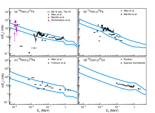
Figure 1: (Color online) Comparison of measured (n,$\gamma$) cross sections with the minimum and maximum TALYS predictions for (a) ⁵⁶Fe(n,$\gamma$), data from Refs. macklin1964 ; allen1976 ; shcherbakov1977 ; (b) ⁵⁷Fe(n,$\gamma$), data from Refs. macklin1964 ; allen1977 ; (c) ⁵⁸Fe(n,$\gamma$), data from Refs. trofimov1985 ; allen1980 , and (d) ⁵⁹Co(n,$\gamma$), data from Refs. trofimov1985 ; allen1980 .

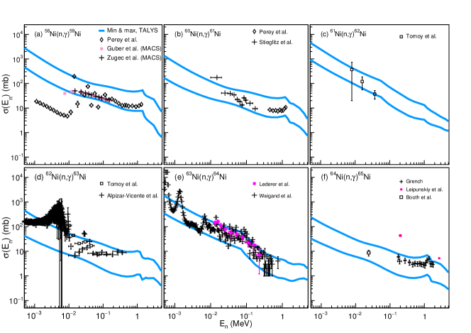
Figure 2: (Color online) Same as Fig. 1 for (a) ⁵⁸Ni(n,$\gamma$), data from Refs. zugec2014 ; perey1993 ; guber2010 ; (b) ⁶⁰Ni(n,$\gamma$), data from Refs. stieglitz1971 ; perey1982 ; (c) ⁶¹Ni(n,$\gamma$), data from Ref. tomyo2005 , (d) ⁶²Ni(n,$\gamma$), data from Refs. tomyo2005 ; alpizar2008 , (e) ⁶³Ni(n,$\gamma$), data from Refs. lederer2014 ; weigand2015 , and (f) ⁶⁴Ni(n,$\gamma$), data from Refs. grench1965 ; leipunskiy1958 ; booth1958 .

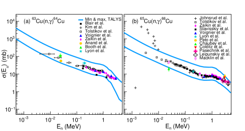
Figure 3: (Color online) Same as Fig. 1 for (a) ⁶³Cu(n,$\gamma$), data from Refs. blair1944 ; voignier1992 ; tolstikov1966 ; zaikin1968 ; kim2007 ; anand1979 ; booth1958 ; lyon1959 ; (b) ⁶⁵Cu(n,$\gamma$), data from Refs. johnsrud1959 ; voignier1992 ; zaikin1968 ; leipunskiy1958 ; pasechnik1958 ; stavisskiy1961 ; tolstikov1964 ; lyon1959 ; macklin1957 ; peto1967 ; chaubey1966 ; colditz1968 .

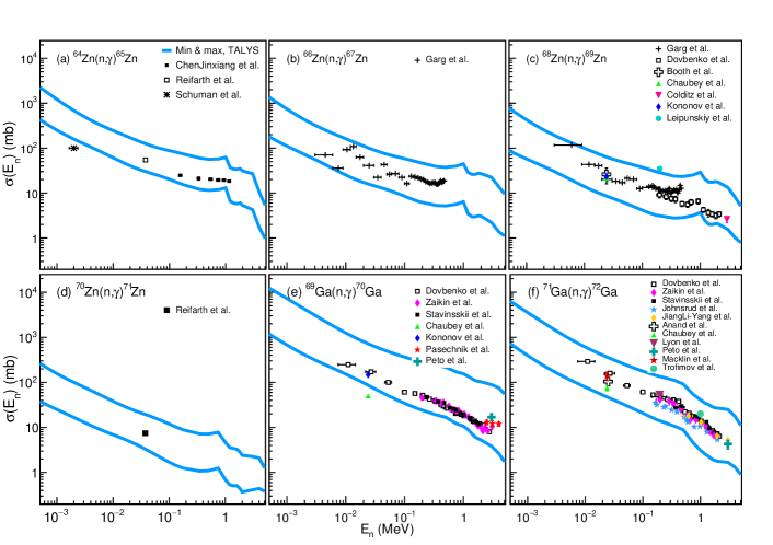
Figure 4: (Color online) Same as Fig. 1 for (a) ⁶⁴Zn(n,$\gamma$), data from Refs. jinxiang1995 ; reifarth2012 ; schuman1970 ; (b) ⁶⁶Zn(n,$\gamma$), data from Ref. garg1981 ; (c) ⁶⁸Zn(n,$\gamma$), data from Refs. leipunskiy1958 ; booth1958 ; chaubey1966 ; colditz1968 ; garg1982 ; dovbenko1973 ; kononov1958 ; (d) ⁷⁰Zn(n,$\gamma$), data from Ref. reifarth2012 ; (e) ⁶⁹Ga(n,$\gamma$), data from Refs. dovbenko1969 ; zaikin1971 ; stavisskii1959 ; chaubey1966 ; kononov1958 ; pasechnik1958 ; peto1967 ; (f) ⁷¹Ga(n,$\gamma$), data from Refs. johnsrud1959 ; dovbenko1969 ; zaikin1971 ; stavisskii1959 ; liyang2012 ; anand1979 ; chaubey1966 ; lyon1959 ; macklin1957 ; peto1967 ; trofimov1987 .

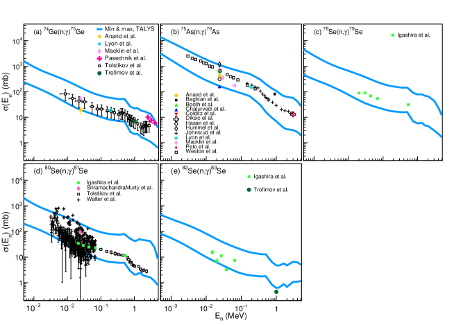
Figure 5: (Color online) Same as Fig. 1 for (a) ⁷⁴Ge(n,$\gamma$), data from Refs. tolstikov1967 ; pasechnik1958 ; anand1979 ; lyon1959 ; macklin1957 ; trofimov1987 ; (b) ⁷⁵As(n,$\gamma$), data from Refs. johnsrud1959 ; anand1979 ; booth1958 ; lyon1959 ; macklin1957 ; peto1967 ; colditz1968 ; beghian1949 ; chaturvedi1970 ; diksic1970 ; hasan1968 ; hummel1951 ; macklin1963 ; weston1960 ; (c) ⁷⁸Se(n,$\gamma$), data from Ref. igashira2011 ; (d) ⁸⁰Se(n,$\gamma$), data from Refs. tolstikov1967 ; igashira2011 ; sriramachandramurty1973 ; walter1984 ; (e) ⁸²Se(n,$\gamma$), data from Refs. trofimov1987 ; igashira2011 .

We have employed the nuclear-reaction code TALYS-1.8 TALYS_16 ; koning12 to calculate radiative neutron-capture cross sections of Fe, Co, Ni, Cu, Zn, Ga, Ge, As, and Se isotopes where direct measurements are available from the EXFOR database EXFOR . A list of considered nuclei is given in Tab. 1, with references to direct measurements for each case.

The TALYS code treats both direct, pre-equilibrium and compound reactions, where the compound part is often the most important one for radiative neutron capture Xu2014 , provided that the level density at the neutron binding energy of the compound nucleus is fairly high. Roughly, the compound-nucleus part of the reaction cross section for radiative neutron capture is given by

$$\sigma_{n\gamma}\propto\mathcal{T}_{n}(E_{n})\rho(E_{n}+S_{n})\mathcal{T}(E_{\gamma}),$$ (1)

where $\mathcal{T}_{n}$ is the neutron transmission coefficient for the target-plus-neutron system determined by the n-OMP, $\rho(E_{n}+S_{n})$ is the NLD in the compound system at the neutron separation energy $S_{n}$ plus the incoming neutron energy $E_{n}$, and $\mathcal{T}(E_{\gamma})$ is the $\gamma$-ray transmission coefficient directly proportional to the $\gamma$SF, $f(E_{\gamma})$, by

$$\mathcal{T}(E_{\gamma})=2\pi E_{\gamma}^{2L+1}f(E_{\gamma}).$$ (2)

Here, $L$ gives the multipolarity of the $\gamma$ transition, which is dominantly dipole ($L=1$) at excitation energies close to $S_{n}$.

For the NLD, TALYS-1.8 has six models implemented:

• The combined constant-temperature ericson1959 plus Fermi gas model bethe1936 as first presented in Ref. gilbert1965 , with parameters as given in the TALYS manual (input keyword ldmodel 1);

• The back-shifted Fermi gas (BSFG) model gilbert1965 with parameters as given in the TALYS manual ( keyword ldmodel 2);

• The generalized superfluid (GSF) model ignatyuk1979 ; ignatyuk1993 (keyword ldmodel 3);

• Calculations based on the Hartree-Fock-Bardeen-Cooper-Schrieffer (HF-BCS) approach demetriou2001 (keyword ldmodel 4);

• Calculations within the Hartree-Fock-Bogoliubov (HFB) plus combinatorial framework goriely2008 (keyword ldmodel 5);
  

• A temperature-dependent HFB plus combinatorial level density hilaire2012 (keyword ldmodel 6).

Note that some of these models have default parameters that are tuned to known data such as the discrete levels at low excitation energy and neutron-resonance spacings at the neutron binding energy. For example, the microscopic models 4–6 are adjusted to these data, if available, by a fit function including an excitation-energy shift and a slope correction. In all cases, we have used the default parameters as implemented in TALYS. Obviously, for very unstable nuclei such data are not available and so the original calculation is used. For more details, see the corresponding references and/or the TALYS-1.8 manual.

For the electric dipole ($E1$) component of the $\gamma$SF, eight models are available:

• The generalized Lorentzian model kopecky_uhl_1990 (keyword strength 1);

• The standard (Brink-Axel) Lorentzian model brink1955 ; axel1962 (keyword strength 2);

• Microscopic calculations within the quasi-particle random-phase approximation (QRPA) for excitations on top of HF-BCS calculations goriely2002 (keyword strength 3);

• QRPA calculations on top of HFB calculations goriely2004 (keyword strength 4);

• The hybrid model of Goriely goriely1998 (keyword strength 5);

• QRPA calculations as in Ref. goriely2004 , but on top of temperature-dependent HFB calculations as in Ref. hilaire2012 (keyword strength 6);

• QRPA calculations combined with temperature-dependent relativistic mean-field calculations daoutidis2010 (keyword strength 7);

• QRPA calculations on top of deformed-basis HFB calculations using the Gogny force martini2016 (keyword strength 8).

For the magnetic dipole ($M1$) strength, we use the default TALYS approach, which corresponds to an $M1$ spin-flip resonance with standard parameterization as of Ref. RIPL3 . Note that we specifically required that no normalization of the $\gamma$SF to known average, radiative widths $\left<\Gamma_{\gamma}\right>$ was done (keyword gnorm 1.). In this way we could assess the predictive power of the models and avoiding a phenomenological re-scaling to match data.

Finally, for the n-OMP, we have used the following two approaches:

• The phenomenological, global parameterization of Koning and Delarouche koning03 (keyword localomp n);

• The semi-microscopic optical potential of the Jeukenne-Lejeune-Mahaux (JLM) type bauge2001 (keyword jlmomp y).

In most cases, the JLM potential is within 20-30% of the Koning-Delarouche potential. We also note that the JLM potential is typically lower than the Koning-Delarouche one for $E_{n}\approx 1-100$ keV. However, for higher neutron energies, typically above 1 MeV, there is in some cases a cross-over and the JLM potential gives a higher ($n,\gamma$) cross section.

The resulting lower and upper TALYS-1.8 predictions, together with available $(n,\gamma)$ cross-section data, are shown in Figs. 1–5 for the Fe, Co, Ni, Cu, Zn, Ga, Ge, As, and Se isotopes. Overall, the TALYS lower and upper cross sections are of the order of a factor $\sim 5-10$. It is interesting to note that the spread in the measured cross sections are in some cases even larger than a factor of 10; more specifically, this is seen in the ⁷⁵As($n,\gamma$) cross section at $E_{n}\simeq 24$ keV in Fig. 5b. It is also obvious from Table 1 that in general, the standard Lorentzian model is always involved in the maximum TALYS prediction, while the generalized Lorentzian is often a component in the minimum one. On the level-density side the picture is not as clear, although the constant-temperature plus Fermi-gas model is most frequently giving the lowest cross section, while the BSFG and GSF models are often predicting the highest cross section. Regarding the n-OMP, the JLM potential gives typically a lower cross section than the Koning-Delarouche potential as mentioned above; however, there are cases where the opposite is true, in particular ⁷⁴Ge($n,\gamma$)⁷⁵Ge and ⁸⁰Se($n,\gamma$)⁸¹Se.

Further, we see that although the upper and lower limits typically wrap around the data, there are some notable exceptions, such as the ⁵⁸Ni($n,\gamma$) cross section for neutron energies below $\approx 10$ keV, and the resonance region in the ^62,63Ni($n,\gamma$) and ⁸⁰Se($n,\gamma$) cross sections below $\approx 10$ keV. It is maybe not so surprising that the resonance region is not well described, and the ”dip” in the ⁵⁸Ni($n,\gamma$) might indicate that the compound-nucleus part of the cross section is much smaller (about a factor of 10) than what TALYS predicts. This might hint to the necessity of an even more sophisticated treatment of the direct and pre-equilibrium components.

Moreover, we note that the minimum TALYS prediction is consistently lower than the majority of the data, while the maximum cross section is surprisingly close to the experimental data for the case ⁶³Ni($n,\gamma$). This underlines the fact that the phenomenological models are not able to properly catch the underlying nuclear structure explaining the measured cross section. Also, since the calculation basically involves a folding of the NLD, $\gamma$SF, and n-OMP (see Eq. (1), it is not straightforward to test these models based on a cross-section measurement alone; one would need data to probe the NLD, $\gamma$SF, and n-OMP separately to be able to identify the correct input for calculating the cross section.

From the comparison of the minimum and maximum TALYS calculations with data for nuclei in the valley of stability, it is quite striking that the predictive power of these frequently used models is not better than typically a factor $\sim 5-10$. It is in fact rather depressing, as the desired uncertainty for ($n,\gamma$) reaction rates involved in the $r$-process is less than a factor of 10 liddick2016 .

Now that the $r$-process is shown to take place in neutron star mergers, prompt ejecta from compact mergers (e.g., just15 ; foucart2014 ; Kasen2017 ) are believed to be rather cold and an ($n,\gamma$)–($\gamma,n$) equilibrium will never be reached arnould2007 . Hence, the ($n,\gamma$) rates play a crucial role. In addition, post-merger neutrino and viscously driven outflows just15 are believed to provide a hot, high-entropy environment, where ($n,\gamma$) reaction rates would mainly be important in the freeze-out phase of the ($n,\gamma$)–($\gamma,n$) equilibrium (e.g., Ref. mumpower2016 ). In either case, it is clear that there is an urgent need to pin down the underlying quantities and improve the model predictions. Considering also that the models should be able to handle exotic nuclei away from stability, the only viable solution seems to be microscopic approaches arnould2007 – both for the NLD, $\gamma$SF and n-OMP as well as for the description of the reaction mechanisms.

In the following, we examine the uncertainties in predicted ($n,\gamma$) reaction rates for neutron-rich nuclei of the elements Fe, Co, Ni, Cu, Zn, Ga, Ge, As, and Se. In particular, we focus on the cases with the highest sensitivity measures according to Ref. surman2014 .

III Reaction rate calculations for neutron-rich nuclei

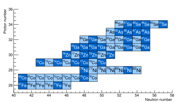
Figure 6: (Color online) Considered cases for investigating the variation in ($n,\gamma$) reaction rates. The cases with sensitivity measure higher than 10 according to Ref. surman2014 are marked in dark blue.

The authors of Ref. surman2014 , as shown in their Fig. 7 and Table II, have identified certain ($n,\gamma$) reaction rates to be of particular importance, even for a large variety of astrophysical conditions. In their study, the ($n,\gamma$) reaction rates were taken from the JINA REACLIB library JINA-REACLIB and scaled up and down with a factor of 10, spanning an uncertainty range of a factor of 100 relative to the JINA REACLIB recommended rates. Surman et al. surman2014 also define a sensitivity measure given by

$$F=100\times\sum_{A}\left|X(A)-X_{\mathrm{baseline}}(A)\right|,$$ (3)

where $X_{\mathrm{baseline}}(A)$ are the final mass fractions for the baseline nuclear-network calculations for a given set of astrophysical conditions (entropy per baryon, dynamic timescale, and the electron fraction). Correspondingly, $X(A)$ represent the final mass fractions for the simulation where the ($n,\gamma$) rates are changed up or down by a factor of 10. In this way, combining the results from 55 different astrophysical trajectories that showed significant sensitivity to neutron-capture rates, cases with particular importance for this range of trajectories (i.e. astrophysical conditions) were identified.

In this section, we investigate what uncertainties TALYS predicts using all possible combinations of level-density and $\gamma$SF models for the rates of the considered moderately neutron-rich nuclei shown in Fig 6. The ”target” nuclei marked in dark blue are the ones with sensitivity measure higher than 10 according to Ref. surman2014 . We also vary the n-OMP as well as the mass models available in TALYS, which are:

• The Duflo-Zuker mass formula duflo1995 (keyword massmodel 0);

• The Möller table moller1995 (keyword massmodel 1);

• The Skyrme-HFB calculations described in Ref. goriely2009 , where an unprecedented rms deviation with experimental masses for a mean-field approach of $<0.6$ MeV is achieved (keyword massmodel 2);

• The Gogny-D1M HFB calculations of Ref.[REF] (keyword massmodel 3).

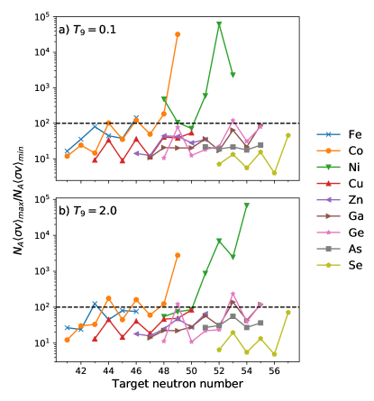
Figure 7: (Color online) Ratios of the maximum and minimum ($n,\gamma$) reaction rates calculated with TALYS. The ratios are taken at temperatures (a) $T=0.1$ GK and (b) $T=2$ GK in the astrophysical environment. The dashed line indicates the considered variation in Ref. surman2014 of a factor 100. In a) the data point of the ⁸²Ni($n,\gamma$) ratio is not included due to the TALYS minimum rate being zero.

In Fig. 7, the ratio of the maximum and minimum ($n,\gamma$) reaction rates calculated with TALYS is shown for the cases in Fig. 6. We see that the ratio is typically a factor $\sim 10-100$, but there are cases that are even more extreme with a factor of $\sim 10^{3}-10^{5}$ such as: a) ⁷⁶Co($n,\gamma$) and ^76,79,80,81Ni($n,\gamma$) for $T=0.1$ GK and b) ⁷⁶Co($n,\gamma$) and ^79,80,81,82Ni($n,\gamma$) for $T=2$ GK. This means that the actual variation in reaction rates could be even larger than the factor of 100 considered in Ref. surman2014 . For the particularly important cases with high sensitivity measure, we see that for $T_{9}=0.1$, ⁸¹Ni($n,\gamma$) varies with a factor of $\sim 2000$, ⁷⁶Ni($n,\gamma$) varies with a factor of $\sim 500$ and ⁷⁵Co($n,\gamma$) vary by approximately by a factor 200. For higher temperatures of $T_{9}=2.0$, ⁸¹Ni($n,\gamma$) varies by a factor $\sim 2000$ and ⁸⁵Ge($n,\gamma$) vary by $\sim 200$. The data point of the ⁸²Ni($n,\gamma$) rate at $T=0.1$ is not included in Fig. 7 due to the TALYS minimum rate being zero.

Further, we compare the TALYS results with the JINA REACLIB rates for the cases of interest (see Fig. 6). In Fig. 8, the ratio of the maximum TALYS rates over the JINA REACLIB rates multiplied with a factor 10 are shown, i.e. we are comparing with the upper limit used in Ref. surman2014 .

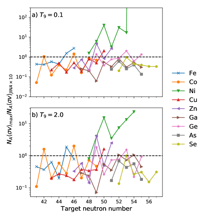
Figure 8: (Color online) Ratios of the maximum ($n,\gamma$) reaction rates calculated with TALYS versus the JINA REACLIB rates multiplied by a factor of 10 for the cases shown in Fig 6. The ratios are taken at temperatures (a) $T=0.1$ GK and (b) $T=2$ GK in the astrophysical environment.

In general, the maximum TALYS rates are smaller than or similar to the JINA REACLIB rates multiplied by 10. At $T_{9}=0.1$, for the cases ^78,80,81Ni($n,\gamma$) the TALYS maximum rates are a factor $\sim 400$, $\sim 300$ and $\sim 160$ respectively, bigger than the JINA REACLIB rates. However, of these three cases only ⁸¹Ni($n,\gamma$) is considered important for the final abundances according to surman2014 .

Another extreme case is the ⁸²Ni($n,\gamma$) reaction (off-scale in Fig. 8a), which for the default JINA REACLIB rate is practically zero ($\sim 10^{-35}$ cm³ $s^{-1}$ mol^-1). That said, the prediction of this rate is extremely sensitive to which mass model is used; the $Q$-value varies from $-0.58$ MeV (FRDM mass input) to $1.09$ MeV (ETSFIQ mass input) – for the latter the JINA REACLIB rate is $\approx 700$ cm³ $s^{-1}$ mol^-1.

For the most important cases (marked dark blue in Fig. 6), we see that the ⁶⁸Co($n,\gamma$) and ⁸⁰Ga($n,\gamma$) maximum TALYS rate is much smaller than the JINA REACLIB rate by about a factor of $\sim 15$ and $\sim 20$ respectively. On the other hand, the maximum TALYS rates for the sensitive cases of ⁷⁹Cu($n,\gamma$), ^79,81Zn($n,\gamma$), ⁸⁵Ge($n,\gamma$) are less than a factor $\sim 10$ larger than the corresponding JINA REACLIB rates, while the maximum TALYS rate of ⁸¹Ni($n,\gamma$) is a factor $\sim 20$ larger than the corresponding JINA REACLIB rates.

For a higher temperature of the astrophysical environment with $T_{9}=2.0$, most of the rates seem to less than 10 times smaller or larger than the maximum JINA rates used in Ref. surman2014 . The largest deviations of the sensitive rates are in the the maximum TALYS rates of ⁸¹Ni($n,\gamma$) that are around $\sim 15$ times larger than the JINA REACLIB rates and for ⁶⁸Co($n,\gamma$) and ⁸⁰Ga($n,\gamma$) that are 10 times smaller than the maximum JINA rate considered in Ref. surman2014 .

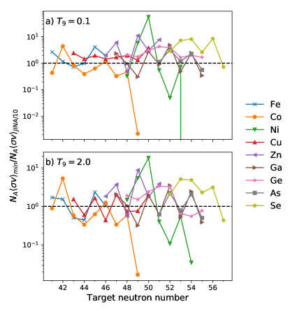
Figure 9: (Color online) Ratios of the minimum ($n,\gamma$) reaction rates calculated with TALYS versus the JINA REACLIB rates divided by a factor of 10 for the cases shown in Fig 6. The ratios are taken at temperatures (a) $T=0.1$ GK and (b) $T=2$ GK in the astrophysical environment.

Next, we compare the minimum TALYS rates with the JINA REACLIB rates divided by a factor of 10, i.e. the lower limit considered in surman2014 . This ratio is shown in Fig. 9 where we see a large variation in the estimated minimum rates. For $T_{9}=0.1$, the most extreme cases are ⁷⁶Co($n,\gamma$) and ⁸⁰Ni($n,\gamma$) where the lower rates from TALYS are a factor of $\sim 10$ and $\sim 1000$ smaller than the lower JINA REACLIB rates. In addition, the case ⁸²Ni($n,\gamma$) is completely off-scale in Fig. 9) because of the nearly zero minimum TALYS rate. On the other hand, the TALYS minimum rate for ⁷⁸Ni($n,\gamma$) is more than a factor of 10 larger than the JINA REACLIB lower rate.

At $T_{9}=2.0$, the overall trend is a spread around the ratio of 1, the TALYS minimum rates are about equal to the JINA REACLIB rates within a factor of $\approx 10$. In particular ⁷⁶Co($n,\gamma$) and ^80,82Ni($n,\gamma$) have a factor of $\sim 10-100$ lower rates while ⁷⁸Ni($n,\gamma$) have a factor of $\sim 200$ higher rate than the JINA REACLIB reaction rate. None of the rates with high sensitivity measure considered in Ref. surman2014 have a deviation of more than a factor of 10 up or down at this astrophysical temperature.

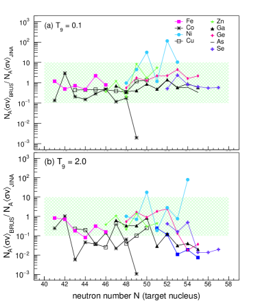
Figure 10: (Color online) Ratios of BRUSLIB ($n,\gamma$) reaction rates versus JINA REACLIB for the cases shown in Fig 6. The ratios are taken at temperatures (a) $T=0.1$ GK and (b) $T=2$ GK in the astrophysical environment. The shadowed band indicates a factor of 100 deviation (factor 10 up or down) as used in the sensitivity study by Ref. surman2014 . In a) the data point of the ⁸²Ni($n,\gamma$) ratio is not included due to the JINA REACLIB rate being extremely low.

Now, we would like to investigate the variation between the JINA REACLIB and BRUSLIB rates, since both these libraries are frequently used in $r$-process reaction network calculations. The result is shown in Fig. 10. We see that for $T_{9}=0.1$, most of the reaction rates are within a factor of 100, except for the cases ⁷⁶Co($n,\gamma$) and ^78,80Ni($n,\gamma$). In addition, the point of the ⁸²Ni($n,\gamma$) ratio is not included in Fig. 10 due to the JINA REACLIB rate being close to zero. For $T_{9}=2.0$ the situation is different, with many BRUSLIB rates being more than a factor 10 smaller than the JINA REACLIB ones. Again focusing on the cases with the highest sensitivity measure, the ⁷⁵Co, ^74,77Cu, ^84,86Ga($n,\gamma$), ⁸⁷Ge($n,\gamma$), ^86,87,88As($n,\gamma$) and ^89,91Se($n,\gamma$) BRUSLIB rates are up to a factor $\approx 10^{-2}$ smaller than the JINA REACLIB predictions.

Further, we consider the possible impact of an enhanced probability for emitting low-energy $\gamma$ rays. At present, there is not so much experimental information on this feature, and we have chosen to implement it as a magnetic-dipole component of the $\gamma$SF following several recent shell-model results schwengner2013 ; brown2014 ; schwengner2017 . Further, we make use of the phenomenological description of the ⁷⁰Ni low-energy $\gamma$SF liddick2016 ; larsen2017 parameterized as

$$f_{\mathrm{up}}(E_{\gamma})=C\exp\left[-\eta E_{\gamma}\right]$$ (4)

following e.g. Ref. renstrom2016 . We apply $C=1.\cdot 10^{-7}$ MeV^-3 and $\eta=1.4$ MeV^-1 in accordance with the ⁷⁰Ni data.

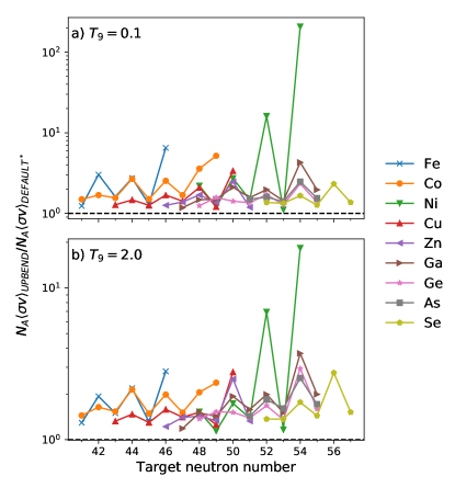
Figure 11: (Color online) Ratios of ($n,\gamma$) reaction rates with and without the low-energy enhancement (upbend) for the cases shown in Fig 6 with the BRUSLIB-like TALYS input (bruslib*). The ratios are taken at temperatures (a) $T=0.1$ GK and (b) $T=2$ GK in the astrophysical environment.

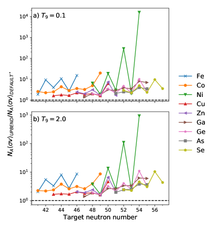
Figure 12: (Color online) Ratios of ($n,\gamma$) reaction rates with and without the low-energy enhancement for the cases shown in Fig 6 with the TALYS default input. The ratios are taken at temperatures (a) $T=0.1$ GK and (b) $T=2$ GK in the astrophysical environment.

To see the influence of this low-energy enhancement on the reaction rates, we have added the $M1$ component in Eq. (4) to the TALYS $\gamma$SF models. In particular, we have used input as close as possible to BRUSLIB BRUSLIB , i.e. the BSk17/HFB-17 mass model (massmodel 2 goriely2009 ) – BRUSLIB uses a similar Skyrme force, BSk24, with slightly better rms deviation for the masses of 0.55 MeV gorielymass2013 – the same NLD (ldmodel 5 goriely2008 ) and $E1$ $\gamma$SF (strength 4 goriely2004 ). In Fig. 11, the ratio of the reaction rates with (upbend) and without (bruselib*) the low-energy enhancement is shown for the cases under study. We see that the low-energy enhancement does lead to an increase in the reaction rates, but in general not more than a factor $\approx 2-20$ for the nuclei studied here. The most extreme point is ⁸²Ni($n,\gamma$) where the upbend rate is $\sim 200$ and $\sim 20$ times larger than the the rate without the enhancement for the astrophysical temperatures of $T=0.1$ and $T=2.0$ respectively. Hence, we see that the upbend always leads to an increase in the rates and represents another uncertainty combined with the uncertainties of varying the $\gamma$SF and NLD models.

We also compared the effect of including the low-energy enhancement in the $\gamma$SF using the default input parameters in TALYS: ldmodel 1, strength 1, localomp n, massmodel 2. The result is shown in Fig. 12 and follow a similar trend to the BRUSLIB-like factors shown in Fig. 11. Again, the enhancement is in general leading to higher rates, but the TALYS default input result in a larger upbend over no upbend ratio. Here, the ^80,82Ni the rates increase by a factor $\approx 300$ and $\approx 10^{4}$, respectively, for $T_{9}=0.1$, and $\approx 100$ and $\approx 1000$ for $T_{9}=2.0$. The main reason for this is that the default $\gamma$SF model, the generalized Lorentzian model kopecky_uhl_1990 is dependent on the nuclear temperature as $T_{f}\approx\sqrt{E_{f}/a}$, where $T_{f}$ is the temperature at final excitation energy $E_{f}=E_{i}-E_{\gamma}$ and $a$ is the level-density parameter. When the neutron separation energy goes down, so does $E_{f}$ and the temperature, and the $E1$ strength is reduced as well. Hence, including a low-energy enhancement as parameterized in Eq. (4) will strongly increase the $\gamma$SF and consequently the ($n,\gamma$) reaction rate. Also, we note that the effect is most significant for the Fe and Ni cases where the compound nucleus is odd, i.e. with a low neutron separation energy.

Now, we would like to highlight some special cases where the reaction rates from the libraries and the TALYS predictions deviate in a particular way.

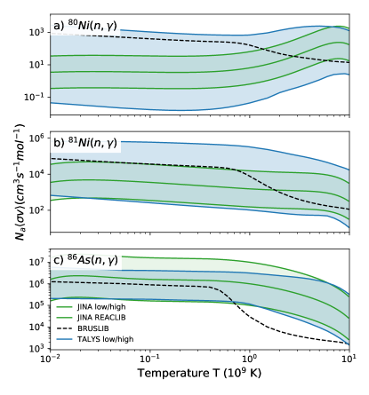
Figure 13: (Color online) Reaction rates for (a) ⁸⁰Ni($n,\gamma$), (b) ⁸¹Ni($n,\gamma$), and (c) ⁸⁶As($n,\gamma$) (see text). The shaded green band indicates the JINA REACLIB multiplied by a factor of 10 up and down and the shaded blue band indicates the TALYS minimum and maximum rates.

In Fig. 13, the reaction rates of ^80,81Ni($n,\gamma$) and ⁸⁶As($n,\gamma$) are shown. In all, we observe very different rates from JINA REACLIB and TALYS as compared to BRUSLIB at high temperatures. Except for a very few crossings, the JINA REACLIB rates scaled with a factor 10 up or down are contained within the TALYS maximum and minimum rates. In general, the BRUSLIB rates have a different shape than the JINA REACLIB and TALYS rates. For instance we see that for ⁸⁰Ni($n,\gamma$), the JINA REACLIB and TALYS rates increases significantly for $T_{9}>1$, with a peak around $T_{9}\approx 7-8$, while in contrast, the BRUSLIB rate decreases for $T_{9}>1$.

One should keep in mind that there is a reported error in the logarithmic energy grid in one of the TALYS subroutines, ’partfunc.f’, for TALYS versions 1.4–1.8 as described in the manual. This error is avoided in the current calculations by enforcing a linear energy grid for the astrophysical rate calculations (keyword equidistant y). However, this error is very likely present in the BRUSLIB calculations, and could be the reason behind the different shapes of the rates at higher temperatures.

IV Conclusions and outlook

In this work we have investigated theoretical predictions of astrophysical ($n,\gamma$) cross sections and reaction rates for Fe, Co, Ni, Cu, Zn, Ga, Ge, As, and Se isotopes, using the open-source reaction code TALYS. We have found that even for nuclei near the valley of stability, the spread in the predicted cross sections is of the order of $5-10$.

For neutron-rich nuclei, the variation between the lowest and highest ($n,\gamma$) reaction rates calculated with TALYS is typically a factor $10-100$, reaching several orders of magnitude for some cases. We have followed Ref. surman2014 and investigated some key reactions that may have a particularly large impact on the final abundances in the $A\sim 80$ region.

Comparing the TALYS ($n,\gamma$) rates with the much-used JINA REACLIB and BRUSLIB reaction rates, we have seen that there are several cases that display very large deviations, much more than the two orders of magnitude considered in Ref. surman2014 . Further, the low-energy upbend in the $\gamma$ strength function has a non-negligible effect on the rates, although we note that the uncertainties due to other factors such as mass models and level densities may have much bigger effects on the rates.

We conclude that there is a dire need for more data to constrain ($n,\gamma$) reaction rates in this mass region. New experimental techniques such as the surrogate method for neutron rich nuclei kozub2012 and the beta-Oslo method spyrou2014 may provide important pieces of information to verify or exclude certain model inputs.

All the calculated cross sections and reaction rates are available at http://ocl.uio.no/xfiles.

- (1) ”Connecting Quarks with the Cosmos: Eleven Science Questions for the New Century”, Board on Physics and Astronomy, The National Academic Press, 2003.
- (2) E. M. Burbidge, G. R. Burbidge, W. A. Fowler, and F. Hoyle, Rev. Mod. Phys. 29, 547 (1957).
- (3) A. G. W. Cameron, Pub. Astron. Soc. Pac. 69, 201 (1957).
- (4) B. S. Meyer, Annu. Rev. Astronn. Astrophys. 32, 153 (1994).
- (5) M. Arnould, S. Goriely, and K. Takahashi, Phys. Rep. 450, 97 (2007).
- (6) F.-K. Thielemann, A. Arcones, R. Käppeli, M. Liebendörfer, T. Rauscher, C. Winteler, C. Fröhlich, I. Dillmann, T. Fischer, G. Martinez-Pinedo, K. Langanke, K. Farouqi, K.-L. Kratz, I. Panove, and I. K. Korneev, Prog. Part Nucl. Phys. 66, 346 (2011).
- (7) W. Hillebrandt, K. Takahashi, and T. Kodama, Astron. & Astrophys. 52, 63 (1976).
- (8) S. E. Woosley, J. R. Wilson, G. J. Mathews, R. D. Hoffman, and B. S. Meyer, Astr. Phys. J 433, 229 (1994).
- (9) J. M. Lattimer and D. N. Schramm, Astrophys. J. 192, L145 (1974).
- (10) J. M. Lattimer, F. Mackie, D. G. Ravenhall, and D. N. Schramm, Astrophys. J. 213, 225 (1977).
- (11) C. Freiburghaus, S. Rosswog, and F.-K. Thielemann, Astrophys. J. Lett. 525, L121 (1999).
- (12) B. P. Abbott et al., Phys. Rev. Lett. 119, 161101 (2017).
- (13) A. Goldstein et al., Astrophys. J. 848, L14 (2017).
- (14) V. Savchenko et al., Astrophys. J. 848, L15 (2017).
- (15) D. A. Coulter et al., Science 10.1126/science.aap9811 (2017).
- (16) S. Valenti et al., Astrophys. J. 848, L24 (2017).
- (17) E. Pian et al., Nature 551, 67 (2017).
- (18) M. R. Drout et al., Science 358, 1570 (2017).
- (19) D. Kasen, B. D. Metzger, J. Barnes, E. Quataert, and E. Ramirez-Ruiz, Nature 551, 80 (2017).
- (20) H.-T. Janka, Annu. Rev. Nucl. Part. Sci. 62, 407 (2012).
- (21) G. Martínez-Pinedo, T. Fischer, A. Lohs, and L. Huther, Phys. Rev. Lett. 109, 251104 (2012).
- (22) S. Goriely, J.-L. Sida, J.-F. Lemaitre, S. Panebianco, N. Dubray, S. Hilaire, A. Bauswein, and H.-T. Janka, Phys. Rev. Lett. 111, 242502 (2013).
- (23) O. Just, A. Bauswein, R. Ardevol Pulpillo, S. Goriely, H.-T. Janka, Month. Not. Roy. Astron. Soc. 448, 541 (2015).
- (24) S. Goriely and H.-T. Janka, MNRAS 459, 4174 (2016).
- (25) Facility for Rare Isotope Beams at Michigan State University, FRIB.
- (26) Facility for Antiproton and Ion Research in Europe GmbH, FAIR.
- (27) High intensity and Energy-ISOLDE at CERN, HIE-ISOLDE.
- (28) C. Travaglio, F.K. Röpke, R. Gallino, W. Hillebrandt, Astrophys. J. 739, 93 (2011).
- (29) R. Surman, M. Mumpower, R. Sinclair, K. L. Jones, W. R. Hix, and G. C. McLaughlin, AIP Advances 4, 041008 (2014).
- (30) M. R. Mumpower, R. Surman, G. C. McLaughlin, and A. Aprahamian, Prog. Part. Nuc. Phys. 86, 86 (2016).
- (31) A. J. Koning, S. Hilaire and M. C. Duijvestijn, ”TALYS-1.8”, Proceedings of the International Conference on Nuclear Data for Science and Technology, April 22-27, 2007, Nice, France, editors O. Bersillon, F. Gunsing, E. Bauge, R. Jacqmin, and S. Leray, EDP Sciences, 2008, p. 211-214.
- (32) A. J. Koning and D. Rochman, Nuclear Data Sheets 113, 2841 (2012).
- (33) A. Voinov et al., Phys. Rev. Lett. 93, 142504 (2004).
- (34) M. Guttormsen et al., Phys. Rev. C 71, 044307 (2005).
- (35) A. C. Larsen, R. Chankova, M. Guttormsen, F. Ingebretsen, S. Messelt, J. Rekstad, S. Siem, N.U.H. Syed, and S.W. Ødegaard, Phys. Rev. C 76, 044303 (2007).
- (36) T. Renstrøm et al., Phys. Rev. C 93, 064302 (2016).
- (37) M. Wiedeking et al., Phys. Rev. Lett. 108, 162503 (2012).
- (38) A. C. Larsen and S. Goriely, Phys. Rev. C 82, 014318 (2010).
- (39) S. N. Liddick et al., Phys. Rev. Lett. 116, 242502 (2016).
- (40) A.C. Larsen et al., in preparation (2017).
- (41) A. C. Larsen et al., Phys. Rev. Lett. 111, 242504 (2013).
- (42) E. Litvinova and N. Belov, Phys. Rev. C 88, 031302(R) (2013).
- (43) R. Schwengner, S. Frauendorf, and A. C. Larsen, Phys. Rev. Lett. 111, 232504 (2013).
- (44) B. Alex Brown and A. C. Larsen, Phys. Rev. Lett. 113, 252502 (2014).
- (45) R. Schwengner, S. Frauendorf, and B. A. Brown, Phys. Rev. Lett. 118, 092502 (2017).
- (46) K. Sieja, Phys. Rev. Lett. 119, 052502 (2017).
- (47) R. H. Cyburt et al., Astrophys. J. Suppl. Ser. 189, 240 (2010); available at https://groups.nscl.msu.edu/jina/reaclib/db/.
- (48) M. Arnould, S. Goriely, Nucl. Phys. A777, 157 (2006). The Brussels Nuclear Library for Astrophysics Applications – BRUSLIB, maintained by Institut d’Astronomie et d’Astrophysique, Université Libre de Bruxelles; available at http://www.astro.ulb.ac.be/bruslib/.
- (49) N. Otuka et al., Nuclear Data Sheets 120, 272 (2014); Experimental Nuclear Reaction Data (EXFOR), database version of July 2015; https://www-nds.iaea.org/exfor/exfor.htm.
- (50) Y. Xu, S. Goriely, A. J. Koning and S. Hilaire, Phys. Rev. C 90, 024604 (2014).
- (51) R. L. Macklin et al., Phys. Rev. 136, 695 (1964).
- (52) B. J. Allen et al., Nucl. Phys. A 269, 408 (1976).
- (53) O. A. Shcherbakov et al., Prog. Yadernye Konstanty 25, 51 (1977).
- (54) B. J. Allen, A. R. De L. Musgrove, R. Taylor, and R. L. Macklin, Meeting on Neutr. Data of Struct. Mat., p.476, Geel 1977.
- (55) Yu. N. Trofimov, Atomnaya Energiya 58, 278 (1985).
- (56) B. J. Allen and R. L. Macklin, Jour. of Phys. G 6, 381 (1980).
- (57) A. Paulsen et al., Zeitschrift fuer Physik 205, 226 (1967).
- (58) R. R. Spencer and R. L. Macklin, Nuclear Science and Engineering 61, 346 (1976).
- (59) P. Zugec et al., Phys. Rev. C 89, 014605 (2014).
- (60) C. M. Perey, F. G. Perey, J. A. Harvey, N. W. Hill, N. M. Larson, R. L. Macklin, and D. C. Larson, Phys. Rev. C 47, 1143 (1993).
- (61) K. H. Guber, H. Derrien, C. L. Leal, G. Arbanas, D. Wiarda, P. E. Koehler, and J. A. Harvey, Phys. Rev. C 82, 057601 (2010).
- (62) R. G. Stieglitz, R. W. Hockenbury, and R .C. Block, Nucl. Phys. A163, 592 (1971).
- (63) C. M. Perey, J. A. Harvey, R. L. Macklin, R. R. Winters, and F. G. Perey, Oak Ridge National Lab. Reports No. 5893 (1982).
- (64) A. Tomyo et al., Astrophysical Journal Letters 623, L153 (2005).
- (65) Yu. P. Popov et al., Yad. Fiz. 63, 583 (2000).
- (66) A. M. Alpizar-Vicente et al., Phys. Rev. C 77, 015806 (2008).
- (67) C. Lederer et al., Phys. Rev. C 89, 025810 (2014); erratum Phys. Rev. C 92, 199903(E) (2015).
- (68) M. Weigand et al., Phys. Rev. C 92, 045810 (2015).
- (69) H. A. Grench, Phys. Rev. 140, 1277 (1965).
- (70) A. I. Leipunskiy et al., Second International At. En. Conf., 15, 50(2219), Geneva 1958.
- (71) R. Booth, W. P. Ball, and M. H. MacGregor, Phys. Rev. 112, 226 (1958).
- (72) J. M. Blair et al., Los Alamos Scientific Lab. Reports 95 (1944).
- (73) J. Voignier et al., Nuclear Science and Engineering 112, 87 (1992).
- (74) V. A. Tolstikov et al., Atomnaya Energiya 21, 45 (1966).
- (75) G. G. Zaikin et al., Atomnaya Energiya 25, 526 (1968).
- (76) G. D. Kim, H. J. Woo, H. W. Choi, N. B. Kim, T. K. Yang, J. H. Chang, K. S. Park, Journal of Radioanalytical and Nuclear Chemistry 271, 553 (2007).
- (77) R. P. Anand, M. L. Jhingan, D. Bhattacharya, E. Kondaiah, Nuovo Cimento A 50, 247 (1979).
- (78) W. S. Lyon, R. L. Macklin, Phys. Rev. 114, 1619 (1959).
- (79) R. L. Macklin, N. H. Lazar, W. S. Lyon, Phys. Rev. 107, 504 (1957).
- (80) G. Peto, Z. Milligy, I. Hunyadi, Journal of Nuclear Energy 21, 797 (1967).
- (81) A. K. Chaubey, M. L. Sehgal, Phys. Rev. 152, 1055 (1966).
- (82) J. Colditz, P. Hille, Oesterr. Akad. Wiss., Math-Naturw. Kl., Anzeiger 105, 236 (1968).
- (83) A. E. Johnsrud et al., Phys. Rev. 116, 927 (1959).
- (84) M. V. Pasechnik et al., Second International At. En. Conf., 15, 18(2030), Geneva 1958.
- (85) Ju. Ya. Stavisskiy et al., Atomnaya Energiya 10, 508 (1961).
- (86) V. A. Tolstikov et al., Atomnaya Energiya 17, 505 (1964).
- (87) Chen Jinxiang et al., Chinese Journ. of Nuclear Physics 17, 342 (1995).
- (88) R. Reifarth, S. Dababneh, M. Heil, F. Käppeler, R. Plag, K. Sonnabend, E. Uberseder, Phys. Rev. C 85, 035802 (2012).
- (89) R. P. Schuman, R. L. Tromp, Idaho Nuclear Corp. Reports No. 1317, 39 (1970).
- (90) J. B. Garg, V. K. Tikku, J. A. Harvey, R. L. Macklin, and J. Halperin, Phys. Rev. C 24, 1922 (1981).
- (91) J. B. Garg, V. K. Tikku, J. A. Harvey, J. Halperin, R. L. Macklin, Phys. Rev. C 25, 1808 (1982).
- (92) A. G. Dovbenko et al., 2. Conf. on Neutron Physics, Kiev 1973, 3, 138 (1974).
- (93) V. N. Kononov, Yu. Ya. Stavisskiy, V. A. Tolstikov, Atomnaya Energiya 5, 564 (1958).
- (94) A. G. Dovbenko et al., Soviet Atomic Energy 26, 82 (1969).
- (95) G. G. Zaikin et al., Ukrainskii Fizichnii Zhurnal 16, 1205 (1971).
- (96) Yu. Ya. Stavisskii et al., Atomnaya Energiya 7, 259 (1959).
- (97) Jiang Li-yang et al., Atomic Energy Science and Technology 46, 641 (2012).
- (98) Yu. N. Trofimov, 1. Int. Conf. on Neutron Physics, Kiev, 14-18 Sep 1987, Vol. 3, 331 (1987).
- (99) V. A. Tolstikov et al., Atomnaya Energiya 23, 566 (1967).
- (100) L. E. Beghian, H. H. Halban, Nature (London) 163, 366 (1949).
- (101) S. N. Chaturvedi, R. Prasad, Nucl. and Solid State Physics Symp., Madurai 1970 Vol. 2, 615 (1970).
- (102) M. Diksic, P. Strohal, G. Peto, P. Bornemisza-Pauspertl, I. Hunyadi, J. Karolyi, Acta Physica Hungarica 28, 257 (1970).
- (103) S. S. Hasan, A. K. Chaubey, M. L. Sehgal, Nuovo Cimento B 58, 402 (1968).
- (104) V. Hummel, B. Hamermesh, Phys. Rev. 82, 67 (1951).
- (105) R. L. Macklin, J. H. Gibbons, T. Inada, Phys. Rev. 129, 2695 (1963).
- (106) L. W. Weston et al., Annals of Physics (New York), Vol. 10, 477 (1960).
- (107) M. Igashira, S. Kamada, T. Katabuchi, M. Mizumoto, J. Nishiyama, M. Tajika, Journal of the Korean Physical Society 59, 1665 (2011).
- (108) M. Sriramachandra Murty, K. Siddappa, J. Rama Rao, Journal of the Physical Society of Japan 35, 8 (1973).
- (109) G. Walter, Kernforschungszentrum Karlsruhe Reports No. 3706 (1984).
- (110) T. Ericson, Nucl. Phys. 11, 481 (1959).
- (111) H. A. Bethe, Phys. Rev. 50, 332 (1936).
- (112) A. Gilbert and A. G. W. Cameron, Can. J. Phys. 43, 1446 (1965).
- (113) A. V. Ignatyuk, K. K. Istekov, and G. N. Smirenkin, Sov. J. Nucl. Phys. 29, 450 (1979).
- (114) A. V. Ignatyuk, J. L. Weil, S. Raman, and S. Kahane, Phys. Rev. C 47, 1504 (1993).
- (115) P. Demetriou and S. Goriely, Nucl. Phys. A 695, 95 (2001).
- (116) S. Goriely, S. Hilaire, and A. J. Koning, Phys. Rev. C 78, 064307 (2008).
- (117) S. Hilaire, M. Girod, S. Goriely, and A. J. Koning, Phys. Rev. C 86, 064317 (2012).
- (118) J. Kopecky and M. Uhl, Phys. Rev. C 41, 1941 (1990).
- (119) D. M. Brink, Ph.D. thesis, Oxford University, 1955.
- (120) P. Axel, Phys. Rev. 126, 671 (1962).
- (121) S. Goriely, E. Khan, Nucl. Phys. A 706, 217 (2002).
- (122) S. Goriely, E. Khan, and M. Samyn, Nucl. Phys. A739, 331 (2004).
- (123) S. Goriely, Phys. Lett. B 436, 10 (1998).
- (124) I. Daoutidis, and S. Goriely, Phys. Rev. C 86, 034328 (2012).
- (125) M. Martini, S. Péru, S. Hilaire, S. Goriely, F. Lechatfois, Physical Review C 94 (2016) 014304
- (126) R. Capote et al., Nucl. Data Sheets 110, 3107 (2009): Reference Input Parameter Library (RIPL-3), available at http://www-nds.iaea.org/RIPL-3/.
- (127) A. J. Koning and J.-P. Delaroche, Nucl. Phys. A713, 231 (2003).
- (128) E. Bauge et al., Phys. Rev. C 63, 024607 (2001).
- (129) Francois Foucart, M. Brett Deaton, Matthew D. Duez, Evan O’Connor, Christian D. Ott, Roland Haas, Lawrence E. Kidder, Harald P. Pfeiffer, Mark A. Scheel, and Bela Szilagyi, Phys. Rev. D 90, 024026 (2014).
- (130) J. Duflo and A.P. Zuker, Phys. Rev. C 52, R23 (1995).
- (131) P.Möller, J.R. Nix, W.D. Myers and W.J.Swiatecki, Atomic Data Nucl. Data Tab. textbf59, 185 (1995).
- (132) S. Goriely, N. Chamel, and J. M. Pearson, Phys. Rev. Lett. 102, 152503 (2009).
- (133) S. Goriely, N. Chamel, and J. M. Pearson, Phys. Rev. C 88, 024308 (2013).
- (134) Kozub et al., Phys. Rev. Lett. 109, 172501 (2012).
- (135) A. Spyrou et al., Phys. Rev. Lett. 113, 232502 (2014).