Why and How to Avoid the Flipped Quaternion Multiplication

Abstract

Over the last decades quaternions have become a crucial and very successful tool for attitude representation in robotics and aerospace. However, there is a major problem that is continuously causing trouble in practice when it comes to exchanging formulas or implementations: there are two quaternion multiplications in common use, Hamilton’s multiplication and its flipped version, which is often associated with NASA’s Jet Propulsion Laboratory. We believe that this particular issue is completely avoidable and only exists today due to a lack of understanding. This paper explains the underlying problem for the popular passive world to body usage of rotation quaternions, and derives an alternative solution compatible with Hamilton’s multiplication. Furthermore, it argues for entirely discontinuing the flipped multiplication. Additionally, it provides recipes for efficiently detecting relevant conventions and migrating formulas or algorithms between them.

Nomenclature

$\mbf x,\mbf M$	vectors and matrices in upper case bold letters. If not specified otherwise matrices are always assumed to be in $\mathbb{R}^{3\times 3}$.
$\mathbb{R}^{k\times 1}$	$\simeq\mathbb{R}^{k}$; implicitly identified $\forall k\in\mathbb{N}$
$\cdot\times\cdot$	cross product
${{\cdot}^{\times}}$	$:\mathbb{R}^{3}\to\mathbb{R}^{3\times 3},\forall\mbf x,\mbf y\in\mathbb{R}^{3}$ : $({{\mbf x}^{\times}})\mbf y={\mbf x}\times\mbf y$
$\mathbb{H}$	$:=(\mathbb{R}^{4},+,\odot)$, quaternions, $(\mbf 1,\mbf i,\mbf j,\mbf k):=(\mbf e_{i})_{i=1}^{4}$
$\mathcal{U}$	$:=\{\mbf q\in\mathbb{H}\,|\,\|\mbf q\|=1\}$, unit length quaternions
$\mbf p\mbf q,\cdot,\odot{}$	Hamilton’s multiplication, i.e. $\mbf i\mbf j=\mbf i\cdot\mbf j=\mbf i\odot\mbf j=\mbf k$
$\otimes$	flipped mult. [1]: $\forall\mbf p,\mbf q\in\mathbb{H}:\mbf q\otimes\mbf p=\mbf p\odot\mbf q$
$\overrightarrow{\mathbf{\mbf q}}\!,{\mathcal{I}(\mbf q)}$	$:\mathbb{H}\to\mathbb{R}^{3},\mbf q=(q_{1},q_{2},q_{3},q_{4})\mapsto(q_{2},q_{3},q_{4})$
${\mathcal{I}^{*}(\mbf x)}$	$:\mathbb{R}^{3}\to\mathbb{H},\mbf x\mapsto x_{1}\mbf i+x_{2}\mbf j+x_{3}\mbf k\Rightarrow\mathcal{I}\circ\mathcal{I}^{*}=\text{id}_{\mathbb{R}^{3}}$
$\mbf q\odot\mbf x,\newline \mbf q\otimes\mbf x$	both quaternion mult. are assumed overloaded for the pairs in $\mathbb{R}^{3}\times\mathbb{R}^{4}$ or $\mathbb{R}^{4}\times\mathbb{R}^{3}$, such that the $\mathbb{R}^{3}$ element is treated as purely imaginary quaternion: e.g. $\forall\mbf q\in\mathbb{R}^{4},\mbf x\in\mathbb{R}^{3}:\mbf x\otimes\mbf q:=\mbf q\odot\mbf x:=\mbf q\odot{\mathcal{I}^{*}(\mbf x)}$
$\bar{\mbf}q$	quaternion conjugation, $\bar{\mbf}q:=(q_{1},-q_{2},-q_{3},-q_{4})$
${\operatorname{SO}(3)}$	$:=(\{\mbf M\in\mathbb{R}^{3\times 3}\,|\,\mbf M^{-1}=\mbf M^{T}\wedge\det(\mbf M)=1\},\cdot)$

I Introduction

“The quaternion [1] is one of the most important representations of the attitude in spacecraft attitude estimation and control.” With these words Malcolm D. Shuster opened his introduction of [2], “The nature of the quaternion” (in 2008). It details on a conventional shift from Hamilton’s original quaternion multiplication, $\odot$, to its flipped version, $\otimes$, he had successfully advocated for in the 1990s - in particular with the very influential [1]. There, the flipped multiplication was called natural and the original was called traditional. Because we consider “natural” too tendentious and because both labels are generally rather unknown we will refer to the former with Shuster’s multiplication and to the latter with Hamilton’s multiplication. Back then, the goal of the introduction was to prevent confusion and mistakes when dealing with chains of rotations (compositions) motivated by the application of spacecraft attitude estimation and control [2]. However, the introduced conventional split with other fields (e.g. mathematics, physics, or computer graphics / visualization) caused a lot of confusion and was a source for potential mistakes in practice at least in other fields, such as robotics. Therefore, in this paper, we advocate to undo this split by only using Hamilton’s original multiplication. At the same time we show how an alternative solution can be used to solve the original problem addressed in [1].

I-A Original problem and Shuster’s solution

The historical problem with Hamilton’s multiplication appeared only together with an arguably arbitrary, specific convention on how to assign direction cosine matrices (DCM), $\mbf C_{S}:\mathcal{U}\to{\operatorname{SO}(3)}$ to unit length quaternions. When using this assignment, as in [1], the product of two quaternions, $\mbf p\odot\mbf q$, would correspond to the product of the two corresponding DCMs, but with reversed order:

$$\forall\mbf p,\mbf q\in\mathcal{U}:\mbf C_{S}(\mbf p\odot\mbf q)=\mbf C_{S}(\mbf q)\cdot\mbf C_{S}(\mbf p).$$ (1)

I.e. the mapping, $\mbf C_{S}$, was not a homomorphism $(\mathcal{U},\odot)\rightarrow({\operatorname{SO}(3)},\cdot)$ but an antihomomorphism, which is generally more surprising and therefore more error-prone and less convenient. Introducing the flipped $\otimes$ is Shuster’s solution to this problem [1]:

$$\mbf p\otimes\mbf q:=\mbf q\odot\mbf p\;\;\Rightarrow\;\;\mbf C_{S}(\mbf p\otimes\mbf q)=\mbf C_{S}(\mbf p)\cdot\mbf C_{S}(\mbf q).$$ (2)

I-B The problem today with Shuster’s solution

Since its introduction, a great fraction of spacecraft literature switched to $\otimes$ [2]. On the other hand virtually the entire rest of the scientific community dealing with quaternions is apparently not following, and partially not even aware of this transition in the spacecraft estimation and control community as we will show in III. Having two different quaternion multiplications in use comes at a significant and continuous cost: formulas and implementations from the two different conventions need translation or adaptation let alone one first must identify which multiplication is used in a given formula or algorithm. The latter can be particularly tedious if the authors are not aware of the two possibilities and hence do not mention which one they use. If a reader is unaware of the split, the discovery that two different quaternion multiplications are in use, and that in fact “the other” was employed, might be made only after several failures, during which the confusion may even have spread to third parties. This was already well observed in [3].

The troubles may be little per subject but they affected and will affect a significant number of scientist and engineers causing delays in the best case. This accumulated cost is particularly large for interdisciplinary domains such as robotics that lean on publications from both conventional worlds, for instance aerospace and computer vision. In fact, in robotics there are several recent publications for each of the two multiplications (see III). It is also a pressing matter because the effort to correct becomes larger with every new implementation or publication using a convention different from what the community agrees on eventually.

I-C Contribution

Given this current situation, it is an interesting question whether the proposed switch was necessary or at least the best of all available options. Or phrased differently, whether some benefit is actually worth this conventional split or whether there is an economical alternative even when considering the effort already invested in the partial transition. Addressing these questions this work provides the following contributions:

• identify the problem of two quaternion multiplications to improve awareness

• investigate the necessity of the flip (2) to solve (1)

• advertise and explain one alternative solution

• demonstrate that this alternative yields more formal similarity to corresponding formulas using matrices

• advocate to discontinue Shuster’s multiplication in favour of Hamilton’s original definition

• provide recipes to detect and migrate between quaternion multiplication conventions

To the best of our knowledge, this is the first work explicitly addressing the ambiguity of quaternion multiplication as a problem and proposing a potential solution. Our work allows for reducing the overall cost associated with having too many competing conventions about the same thing.

I-D Outline

We start with important background information in II. In III, we summarize relevant contributions on quaternion multiplication related conventions, and tabulate their popularity in recent or influential publications. Next, we propose an alternative solution in IV. Then we argue for discontinuing Shuster’s multiplication in V. Lastly, we provide recipes for detecting and migrating rotation quaternion related conventions in VI. Further supplemental information is provided in the appendix.

II Background: Duality of rotation representations

Physical rotations are conceptually rather unambiguous. However, when it comes to describing them, there are two popular ways to do so. The active way is to describe what happens to the rotated body’s points from a fixed world frame’s perspective. The passive way is to describe how coordinates of fixed world points change from the perspective of the rotated body frame. It comes in two flavours, world-to-body (PWTB) and body-to-world (PBTW). The first describes the change from before rotation to after and the second from after to before. We call these options the usage of the mathematical model to describe the physical rotation. Mathematically, the described actions on the observed points have identical properties in all three cases matching precisely the actions of the special orthogonal group (${\operatorname{SO}}$) on the underlying Euclidean space. But because given the same physical rotation, PWTB describes the inverse compared to PBTW, they yield mutually inverse group elements. Despite of being conceptually very different, the active usage yields always the same group element as PBTW. Consequentially we will often not distinguish these two. See App. C for an in-depth discussion of the various ways to use matrices to represent physical rotations.

The crucial consequence is that while every parametrization of the ${\operatorname{SO}}$ can be employed for all usages, switching usage from or to PWTB corresponds to an inversion. We believe that a lack of awareness for this fact ultimately led to the “problem” (1) (see V-E4). The main target audience of this paper are those who favour the PWTB usage because the problem (1) is exclusive for the PWTB usage.

III Literature review

Not many publications discuss the multitude of possible conventions or argue for a specific choice, instead the common way seems to either just assume a convention or define one more or less completely before using it.

III-A Literature on or introducing relevant conventions

III-A1 Aerospace

According to [4] Shuster’s multiplication, $\otimes$, was introduced in [5]. It was later proposed as a standard in [6] according to [7]. Unfortunately, the exact details are impossible for us to reconstruct as NASA is not publishing [6]. In [8] the authors derive a homomorphic composition rule for Euler (symmetric) parameter (ESP) (effectively $\otimes$) and infer a required conjugation from ESP to Hamilton’s quaternions. In IV we are proposing the same quaternion values as alternative solution but with different derivation. According to [1, p.473] (7 years later), the authors of [8] in fact preferred Shuster’s multiplication over Hamilton’s. This indicates that they considered Euler parameter together with Shuster’s multiplication a separate representation distinguished from Hamilton’s quaternions by a conjugation.

In [2] the author describes the transition from Hamilton’s $\odot$ to Shuster’s $\otimes$ for “spacecraft attitude estimation and control” literature : “Hamilton’s approach to quaternions …, seemingly in universal use until the publication of reference [9] and still in almost universal use until the publication of reference [1], which, probably, more than any other work, has been responsible for the change to the natural order of quaternion multiplication in spacecraft attitude estimation and control. This was, in fact, an avowed purpose of the author of reference [1]. But although nearly every writer on spacecraft attitude is aware now of reference [1], which is cited frequently, he or she may not be aware of the inconsistency of reference [1] with many other works on quaternions.”In [1] $\otimes$ is indeed derived as necessity given some requirements, of which one was the correspondence $\mbf C_{S}$. In order to demonstrate a clear trend towards generally adopting the new multiplication order [2] cites recent publications dealing with rotation quaternions: four using Shuster’s multiplication and one using Hamilton’s multiplication. The fact that the first were all aerospace paper and the last a book on applied mathematics might be related to Shuster’s observation in [1], when explaining why mathematicians might not have changed the quaternion multiplication order: “The concern of pure mathematics is not in representing physical reality efficiently but in exploring mathematical structures … As engineers, our interest is in “im-pure” mathematics, contaminated by the needs of practical application.” A major struggle with the quaternion conventions within NASA is reported in [10], including the discussion of a major conventional switch from the official Space Shuttle program to the (American) International Space Station software standard. The author compares these two conventions with a third convention that he calls Robotics. Neither [1] nor [2] are mentioned in [10] despite their apparent relevance. The only easily accessible reference in [10] for quaternions, [11], uses Hamilton’s multiplication and also does not mention Shuster’s work.

The Navigation and Ancillary Information Facility (NAIF), a sub organization of NASA’s Jet Propulsion Laboratory (JPL), uses Hamilton’s multiplication everywhere in their primary software suite called SPICE [12]. In that document, the authors introduce two conventions: SPICE Quaternions, using Hamilton’s multiplication, and Alternate Style Quaternions, using Shuster’s multiplication. They present important formulas in both “styles” and stress intensively how important it is to pay attention to the small difference in the details. The authors use the short terms SPICE quaternions and Engineering quaternions and describe the first with “Invented by Sir William Rowan Hamilton; Frequently used in mathematics and physics textbooks” and the second with “Widely used in aerospace engineering applications” (e.g. cspice/qxq_c).

III-A2 Robotics

In [3] the author proposes a classification of rotation quaternion related conventions based on four binary choices leading to “12 different combinations”. The choice between homomorphic and anti-homomorphic matrix to quaternion conversion (see V-C) is not among these choices. Instead homomorphy is implicitly assumed as a natural requirement. The author also points out two most commonly used conventions, one using Shuster’s and one using Hamilton’s multiplication. The author chooses to use Hamilton’s multiplication because it “… coincides with many software libraries of widespread use in robotics, such as Eigen, ROS, Google Ceres, and with a vast amount of literature on Kalman filtering for attitude estimation using IMUs ([13, 14, 15, 16, 17], and many others).” At the same time PBTW usage is chosen, circumventing the problem (1).

III-B Popularity in influential and recent literature

In Table I we group publications, which are recently dealing with rotation quaternions, by which quaternion multiplication is used, by the type of publication, and the scientific community for books and papers. Of course, this is merely a small selection of corresponding publications in the respective fields.

TABLE I: Popularity of the two multiplications

Type/Community	Hamilton	Shuster
Online encyclopedia	Encyclopedia of Math., Wolfram Mathworld, Planetmath, Britannica, Wikipedia
Mathematics	[14](B!), [18](Ba), [19](Ba), [20](Baw), [21](B-)
Aerospace	[8](B), [22](Bw), [14](B!), [11](B!), [23](w), [24](!)	[5, 1, 4, 25, 26, 27, 28, 29, 30]
Robotics	[31](a), [13](aw), [32](Bw), [16](w), [17](w),​ [3](w), [33](w)	[7], [34], [26], [35], [36]
Mechanics	[37](w), [38](w), [39](Baw), [40](Ba), [41](Ba) [42](Ba)
Control	[23](w), [43](!), [33](w), [44](!)
Computer vision	[31](a), [45](aw), [16](w)
Computer graphics / visualization	[46](!), [45](aw), [47](aw), [48](B!), [20](Baw), [49](-)
Applications and software libraries	Wolfram Mathematica, Matlab’s aerospace(!) and robotics toolbox, C++ library Eigen (see App. E), Google Ceres, Boost, GNU Octave, ROS, NASA’s SPICE (qxq_c, m2q_c)	Microsoft’s DirectXMath Library

Within these constraints the table shows: All relevant online general purpose or mathematical encyclopedias, which we could find, use Hamilton’s multiplication (without mentioning any alternatives). And so do all major software packages. Most of them also use precisely the quaternion to matrix mapping we suggest as part of an alternative solution to (1) in IV. The only scientific communities we could find using Shuster’s multiplication are aerospace and robotics. Both seem to be still divided. Even NASA itself and it’s substructure JPL seem to be divided to this day.

IV Proposed alternative solution

The alternative solution we suggest for the original problem (1) is to use a different correspondence rule, $\mbf C_{H}:\mathcal{U}\ni\mbf q\mapsto\mbf C_{S}(\bar{\mbf}q)$. Assuming we keep fixed how rotation matrices represent rotations, this new correspondence inverts the corresponding quaternion. It also yields the desired homomorphy from quaternions to rotation matrices together with $\odot$ and the usual matrix multiplication:

$$\forall\mbf p,\mbf q\in\mathcal{U}:\mbf C_{H}(\mbf p\odot\mbf q)=\mbf C_{H}(\mbf p)\cdot\mbf C_{H}(\mbf q).$$ (3)

This suggestion might give the wrong negative impression of an “additional” inversion. But it could equally well be that for $\mbf C_{S}$ the “wrong” (inverted) quaternions were chosen. In fact our observations in V-E4 support this interpretation and allow it to be explained as follows: the mistake to use active quaternions in a passive usage scenario led to $\mbf C_{S}$, which in turn led to flipping the multiplication, while choosing appropriate passive quaternions would have lead to $\mbf C_{H}$ and no need to flip the multiplication.

Please note that both solutions yield the usual way to apply the rotation represented by a quaternion (see VI-B2):

$$\forall{\mbf x\in\mathbb{R}^{3},\mbf q\in\mathcal{U}}:\begin{matrix}\mbf C_{H}(\mbf q)\mbf x={\mathcal{I}(\mbf q\odot{\mathcal{I}^{*}(\mbf x)}\odot\mbf q^{-1})}\\ \mbf C_{S}(\mbf q)\mbf x={\mathcal{I}(\mbf q\otimes{\mathcal{I}^{*}(\mbf x)}\otimes\mbf q^{-1})}\end{matrix}$$ (4)

We are going to refer to the $\mbf C_{H}$ rotation quaternions with Hamilton’s rotation quaternions because they yield homomorphy together with Hamilton’s quaternion multiplication (see V-C).

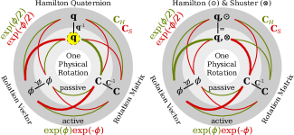
Figure 1: Active (or passive body-to-world; outer ring) and passive (world-to-body; inner ring) representatives of a single physical rotation and their mutual conversions: black lines convert only between active and passive, green convert between different parametrizations, and red additionally invert. The bold lines on the left (Hamilton multiplication only) constitute the homomorphic convention suggested in this paper. It is suitable for everybody preferring passive world-to-body for $\mbf q$ and $\mbf C$. The rare users of passive rotation vectors would entirely remain in the inner circle. Clinging to the green conversion from the common active ${{\boldsymbol{\phi}}}$ to $\mbf q$ even if the quaternion is intended to be employed passively, as done in [1] leads to the situation on the right (using Shuster’s multiplication when employing quaternions passively). This neglects the option of the highlighted passive $\mbf q$ (on the left) and thus requires the flipped multiplication, $\otimes$, and inevitably breaks the symmetry between $\mbf C$ and $\mbf q$ on the right compared to the left.

V Rationale against Shuster’s multiplication

V-A Overview

First of all, it is important to emphasize that the question which quaternion multiplication to use commonly, should be considered as a pragmatic question. Conceptually there is no problem with any of the two multiplications or with having two multiplications commonly used. Having said that, our main argument is as follows:

V-A1 Both multiplications are equally capable and interchangeable for every application

As we explain in V-B one multiplication is as good as the other in terms of applicability. For example to represent rotations. There is a difference for those rare people who use the components of a rotation quaternion intuitively. However, for these we suggest a better alternative in V-G. Having both “available” at the same time does not add extra expressiveness because one can always be substituted by the other with flipped arguments.

V-A2 One of the two multiplications should be discontinued

Having two quaternion multiplications in formulas and software comes at a significant and ongoing cost (see I-B, III), but does not provide benefits (see V-A1).

V-A3 Hamilton’s multiplication is preferable

Hamilton’s multiplication is predominant over all existing publications. This is because i) it is about 150 years older, and ii) Shuster’s multiplication did not spread to mathematics or theoretical physics and probably will never do. The latter arises from the fact that both disciplines have very different needs that typically do not even lead to the original problem (1) as already observed in [1]. To the best of our knowledge it only spread from aerospace to parts of robotics, which has similar needs and is strongly influenced (among others) by aerospace literature. Also, Hamilton’s multiplication is used by the vast majority of current software (libraries) (see Table I). Interestingly this includes the SPICE package developed at NAIF for and as part of the very same JPL at which Shuster’s multiplication was proposed as a standard [6]. These observations make it extremely difficult to discontinue Hamilton’s multiplication instead. Even more so, pure mathematics should be almost impossible to influence in that respect because it is against the very nature of mathematics to change such a definition without an inner-mathematical reason.

Additionally, as we show in V-E3, Hamilton’s multiplication has its benefits over Shuster’s from a formal point of view. These benefits make it less error prone if combined with the alternative quaternion to rotation matrix mapping, $\mbf C_{H}$, which is at least as old and well-known as $\mbf C_{S}$. It is typically used whenever rotations are represented actively or PBTW (see II). Because of that, $\mbf C_{H}$ is also already predominant among existing software implementations (see Table I).

Employing $\mbf C_{H}$ also for the very popular PWTB usage, as we suggest, has a consequence that one could consider its biggest drawback: It introduces the comparatively rarely seen passive quaternion (see Table II, Fig. 1), and thus induces an unusual conversion from an active rotation vector, ${{\boldsymbol{\phi}}}$: $\mbf q({{\boldsymbol{\phi}}})=\exp(-0.5{{\boldsymbol{\phi}}})$. Eventually, the original problem $\eqref{eq:problem}$ leaves two options: i) introducing an unusual quaternion multiplication (Shuster’s solution) or ii) introducing an unusual conversion from the active rotation vector to the (passive) rotation quaternion (used e.g. in [8]). Having only these two options is probably the very difficulty behind the overall struggle and what prevented a standardization so far (see III). Also, general purpose text books do not help resolving this issue as they typically do consider neither i) nor ii) by either accepting antihomomorphy or only consider active / PBTW usage (see III-B).

Our position, in favour of ii), emerges from rephrasing the question equivalently: What should be specific for the passive usage of quaternions when compared to the active usage, their multiplication or the conversion to the active rotation vector? It reveals an immediate argument for ii): the conversion from active rotation vector to passive quaternion should even be expected to be different from its conversion to an active quaternion (compare also II). An argument against i) is that the multiplication is used much more often, because conversions are merely interface operations and usually do not appear where the heavy lifting is done. Also, if we have to chose the multiplication depending on the usage of quaternions to represent rotations, which multiplication is right for other applications? Furthermore, it is very unusual and therefore unexpected that a fundamental algebraic operation such as a multiplication is a matter of dispute and convention, while it is quite common for representations. Finally, the very same question for rotation matrices was answered historically: there is no flipped matrix multiplication in regular use. Instead it is fully accepted that there is an active and a passive rotation matrix mutually inverse and related differently to an active rotation vector. Why not accept the exact same for rotation quaternions while employing them for exactly the same purpose?

V-B Equal capability argument

In this section we explain why both multiplications are equally capable to support V-A1). The migration recipes in VI-B show that any algorithm or formula can be migrated between the two multiplications with very simple steps: just introduce quaternion conjugation at some places and exchange all multiplications. This already shows that both multiplications can provide the same service to the user (writer, reader, programmer), as the migration concepts work in both directions.

The question remains whether one implementation could be computationally more efficient than the other. However, one should easily be convinced that the extra cost for some additional conjugations is negligible for most use cases since it only involves scalar negations. Furthermore, for very performance critical parts of an implementation, the negations can almost always be statically merged into other operations or simplified away mathematically (compare also V-F).

V-C Formal differences

One major problem when writing about representations for rotations is that there are many different representations and for most of them there are multiple conventions concerning their details and mutual relation (see e.g. [1], [3] or App. C). In fact there is not even a reliable agreement on what precisely proper rotations are (e.g. active vs. passive rotations) or — more generally — how to distinguish the different things to represent.

For this section we choose a different approach: we restrict ourselves to the relation between unit quaternions and special orthogonal matrices while leaving open how the latter are used to represent physical rotations or similar. This way the analysis stays general and less complex because most of the usual complexity comes from the how and what to represent. This strategy is possible because there is a common aspect considering all usual ways to model proper physical rotations with matrices: They formulate a one to one relationship with the special orthogonal $\mathbb{R}^{3\times 3}$ matrices, ${\operatorname{SO}(3)}:=\{\mbf C\in\mathbb{R}^{3\times 3}|\mbf C^{T}=\mbf C,\det(\mbf C)=1\}$ with their group operation (matrix multiplication) corresponding to some composition of rotations — just in different ways. The direction cosine matrix used in the introduction as an example is only one possible interpretation of ${\operatorname{SO}(3)}$. See App. C2 for a discussion of all the common interpretations.

This little common ground is already enough to formulate the original problem when restricting it to the relation between unit quaternions, $\mathcal{U}:=\{\mbf q\in\mathbb{H}=(\mathbb{R}^{4},+,\odot),\|\mbf q\|=1\}$, and ${\operatorname{SO}(3)}$ by entirely forgetting about their potential usage. This relation has different meaning depending on which meaning is assigned to $\mathcal{U}$ and ${\operatorname{SO}(3)}$ but all common formal possibilities how to map $\mathcal{U}$ to ${\operatorname{SO}(3)}$ can be analyzed entirely without referring to this meaning. This way a thorough formal comparison becomes more tractable.

Because of this possibility we will, after introducing some essential notions, adopt a purely formal perspective to compare the common different ways for how to map $\mathcal{U}$ to ${\operatorname{SO}(3)}$ and its relation to the quaternion multiplication and rephrase the original problem in that context. This will leave us with two optimal solutions: the one that was suggested in [1] and the one we are proposing to adopt instead. To compare them further we will investigate the relation to the cross product, the rotation vector and the angular velocity in V-E3 and additionally to the active usage in V-E4. These comparison will show significant differences in favour of the solution including Hamilton’s multiplication. After that we are going to verify that non of the other perspectives, numeric, algorithmic and intuition give strong reasons for one of the two option over the other. In particular, we will explain why non of them performs better from any of these other perspectives. This way, overall, our suggestion will remains as preferable.

V-D Essential notions

To support a concise communication in this V-C it is important to clarify some essential notions, namely rotation and convention of rotation representation.

V-D1 Rotation

For the sake of simplicity we refer to 3-dimensional proper rotations or attitude / orientation or coordinate transformations between orthonormal coordinate systems with just rotations. Despite the fact that these are quite different concepts this is possible because for this paper’s cause and arguments their distinction is irrelevant.

V-D2 Partial rotation convention

In order to allow reliable arguments for a claim like both multiplications are equally capable we need some rigorous notion to specify what precisely we compare. As tools for rotation representation the quaternion multiplications do not stand alone. Instead they need to be combined with rules such as how to use them to rotate a vector, which typically involve choosing one of multiple available options (see for example the binary choices of [3]). A set of such rules / determinations is often referred to as convention. What we actually want to compare are classes of such conventions. For instance the class of conventions using Hamilton’s multiplication with the class using Shuster’s multiplication.

One way to support this would be to define the convention notion in a rigorous way. But this is difficult mostly because it is not clear what specifications are necessary for a convention to be complete. In practice it is very different how much authors actually specify when they declare the convention they use in a text. Typically not more than needed for that text, which is highly dependent on the text. This problem we avoid by introducing the new concept of a partial rotation convention or shorter partial convention. They can play the role of convention classes without relying on a rigorous notion of a complete / full convention.

We refer to any set of arbitrary determinations concerning rotation representation, i.e. not necessary in that particular way, with partial rotation convention. These determinations can be explicit or implicit, i.e. logical / mathematical consequences from the explicit determinations. This is quite analogous to the notion of an axiom system for a given domain. Therefore we call the explicit determinations axioms. Examples of such determinations are conversion rules between rotation parametrizations, how a orthogonal matrix is interpreted as rotation, or how to multiply two rotation quaternions. Fortunately it is not necessary for our cause to specify all kind of determinations that can be made by a partial convention.

Consistency

A partial convention not contain contradicting axioms we call a consistent partial convention. One hypothetical non-consistent example could be when a convention includes all conversion rules in the triangle of unit quaternions, orthogonal matrices, and angle axis parameters but converting a quaternion first into angle axis and then into a matrix can yield a different result from when the same quaternion is directly converted to a matrix. We only care for consistent conventions.

Natural partial order

These partial conventions naturally posses a partial order, just like sets induced by their inclusion. We say a partial convention, $C$, is included in another convention, $D$, ($C\subseteq D$), iff the union of their determinations would yield a consistent partial convention and this union would not determine anything more than $D$. This fits well the intuitive expectation that when adding an axiom to a convention it becomes a larger convention. In practice it is sufficient and necessary for $C\subseteq D$ that all axioms of $C$ are also determined by $D$. This makes it particularly easy for a $C$ with only a few axioms.

QM-convention

We call a partial convention that determines a map from unit quaternions to orthogonal matrices and a particular quaternion multiplication a QM-convention. We call a partial convention, $C$ a minimal QM-convention iff it is a QM-convention and minimal with respect to their partial order, i.e. there is no partial convention $\hat{C}\subseteq C$ such that it isn’t also $C\subseteq\hat{C}$. Such a partial convention does not determine anything more than absolutely necessary for a QM-convention. One important fact about partial conventions is that everything that can be inferred from the axioms of a given convention applies to all larger partial conventions. This ultimately makes our investigation of minimal QM-conventions in V-E relevant for the partial conventions used in practice, which are typically (much) larger.

V-E Mathematical / formal perspective

Given a way to represent rotations with matrices there are different approaches to employ unit quaternions, $\mathcal{U}$, as representation for physical rotations. One approach, the matrix-induced method, is to parametrize these matrices with unit quaternions, by specifying a surjective mapping $\mathcal{U}\to{\operatorname{SO}(3)}$, and retrieve the induced rotation representation by the unit quaternions. Others approaches are to model rotations directly with unit quaternions or specify their relation to other available rotations representations. Once a unit quaternion representation is given the conversion to any other representation including any matrix representation can be formally retrieved. Any such conversion from unit quaternion representation to a matrix representation would yield a surjective mapping $\mathcal{U}\to{\operatorname{SO}(3)}$. It must be surjective because the matrices are one to one representations in all cases. I.e. leaving one out would mean missing a physical rotation. Therefore one can find the the same representation applying the matrix-induced approach.

For this section we are adopting the matrix-induced approach because it involves a minimal number of choices while being at least as powerful. We assume the choice for a specific matrix representation to be fixed but unknown to make sure the analysis does not depend on that choice. We are going to compare a set of two mappings only, $\mbf C_{H},\mbf C_{S}$, from $\mathcal{U}$ to ${\operatorname{SO}(3)}$, which can be uniquely defined by (4). To the best of our knowledge, these two mappings constitute effectively all mappings that were found and successfully used in the history of representing physical rotations.

V-E1 Problem formalization

By the means of both mappings the unit quaternions become singularity free parametrizations of ${\operatorname{SO}(3)}$, the Euler-Rodrigues parameters in case of $M_{1}$. The problem, (1), comes with the comparison of matrix and quaternion multiplication, each inducing a Lie-group structure on the respective sets, through $M_{1}$ and $M_{2}$. It turns out that the mappings $\mbf C_{H},\mbf C_{S}$ are - from this algebraic perspective - smooth and surjective group homomorphisms ($\mbf C_{H}$) and antihomomorphisms ($\mbf C_{S}$) respectively from $\mathcal{U}$ to ${\operatorname{SO}(3)}$:

$$\forall{\mbf p,\mbf q\in\mathcal{U}}:\mbf C_{H}(\mbf p\mbf q) =\mbf C_{H}(\mbf p)\mbf C_{H}(\mbf q)\wedge\mbf C_{S}(\mbf p\mbf q)$$ (5)

$$=\mbf C_{S}(\mbf q)\mbf C_{S}(\mbf p)$$

This property follows immediately from the defining property (4), because both multiplications (quaternion and matrix) are associative.

When switching from $(\mathcal{U},\odot)$ to its opposite group $\mathcal{U}^{\text{op}}=(\mathcal{U},\otimes)$ with the flipped multiplication, as suggested by [1], a very similar statement becomes true, with the only difference that — as in general when switching one group to its opposite group – homomorphisms and antihomomorphisms switch places when kept fixed as mappings between the two sets, because the identity mapping between the two is an antiisomorphism.

$$\forall{\mbf p,\mbf q\in\mathcal{U}}:\mbf C_{S}(\mbf p\otimes\mbf q) =\mbf C_{S}(\mbf p)\mbf C_{S}(\mbf q)\wedge\mbf C_{H}(\mbf p\otimes\mbf q)$$ (6)

$$=\mbf C_{H}(\mbf q)\mbf C_{H}(\mbf p)$$

Because $\mathcal{U}$ and $\mathcal{U}^{\text{op}}$ are isomorphic, by means of

$$\psi:\mbf q\mapsto\mbf q^{-1}$$ (7)

and because $\mbf C_{S}=\mbf C_{H}\circ\Psi\wedge\mbf C_{H}=\mbf C_{S}\circ\Psi$ they also switch places with respect to property (4):

$$\forall{\mbf x\in\mathbb{R}^{3}}:\mbf C_{S}(\mbf q)\mbf x=\mbf q\otimes\mbf x\otimes\mbf q^{-1}\wedge\mbf C_{H}(\mbf q)\mbf x=\mbf q^{-1}\otimes\mbf x\otimes\mbf q$$ (8)

The historic problem (1) and action consequently taken can now be phrased as follows: Experience in spacecraft attitude estimation and control showed that dealing with rotation quaternions that behaved antihomomorphic compared to the orthogonal matrices used for the same purpose was error prone and unaesthetic. It was antihomomorphic, because $\mbf C_{S}$ was the mapping used together with Hamilton’s quaternion multiplication, as in the second part of (5). For some reason it was out of question to change the mapping from quaternion to matrix from $\mbf C_{S}$ to $\mbf C_{H}$. And therefore, it was suggested to flip the quaternion multiplication order - the only alternative left besides flipping the matrix multiplication order - to fix the antihomomorphy of (1).

In this paper we are claiming that it would have been better to switch from $\mbf C_{S}$ to $\mbf C_{H}$ instead, see V-A3).

The four possible outcomes of the two binary choices, $(\mbf C,\star)\in\{\mbf C_{H},\mbf C_{S}\}\times\{\odot,\otimes\}$, yield all the minimal QM-conventions included in any of the usual convention used in practice. Hence all considerations concerning those four applies to all convention practically used, only depending on which of these four are included.

From the purely formal perspective it is well understandable that the two homomorphic QM-conventions (HQMC), $(\mbf C_{H},\odot)$ and $(\mbf C_{S},\otimes)$, are favourable over the antihomomorphic QM-conventions, $(\mbf C_{S},\odot)$ and $(\mbf C_{H},\otimes)$. In [3] partial conventions including the antihomomorphic pairs are not even considered possible conventions, because there the choice of the multiplication determines the mapping from quaternions to matrices by assuming the homomorphy through (9), as beyond dispute — and we can only agree with that.

It is also apparent that there is nothing to be gained by choosing one option over the other among the two homomorphic QM-conventions — from this formal perspective. Both fulfill the same and only relevant and desired properties for a homomorphic QM-convention, $(\mbf C,\star)\in\{(\mbf C_{H},\odot),(\mbf C_{S},\otimes)\}$

$$\mbf C(\mbf q)\mbf x ={\mathcal{I}(\mbf q\star\mbf x\star\mbf q^{-1})}$$ (9)

$$\Rightarrow\mbf C(\mbf p\star\mbf q) =\mbf C(\mbf p)\mbf C(\mbf q)$$ (10)

as observed in (4), (6) and (5), (8).

Extension to the entire quaternions algebra

Sometimes derivations or algorithms exploit the fact that the unit quaternions are embedded in the algebra and skew-field of quaternions, $\mathbb{H}$. But even together with this embedding the two options are isomorphic and therefore equally capable. This can be seen as follows. The mapping

$$\Psi:(\mathbb{H},\otimes)\to(\mathbb{H},\odot),\mbf q\mapsto\bar{\mbf}q,$$ (11)

where $\bar{\mbf}q$ denotes the quaternion conjugate of $\mbf q$, is a skew-field isomorphism $(\mathbb{H},\otimes)\to(\mathbb{H},\odot)$. This can be easily verified using the well-known antihomomorphy properties of quaternion conjugation. Furthermore, $\Psi$ is an extension of $\psi$ onto $\mathbb{H}$ in the sense that restriction of $\Psi$ onto $\mathcal{U}$ is $\psi$. Additionally the quaternion norm $\|\cdot\|$ defining $\mathcal{U}$ commutes with $\Psi$. This implies that the embedding relation between $\mathcal{U}$ and $\mathbb{H}$ fully compatible with $\Psi$. Please note that $\Psi$ does not keep the imaginary units $\mbf i,\mbf j,\mbf k$ invariant. Instead they get mapped to their negative.

V-E2 Seeking formal differences that allow for a preference

So far the formal comparison could not yield any preference for one of the two HQMCs. Therefore in this section we are going to discuss the effect of this choice on the relation to additional rotational concepts. Namely the rotation vector and the angular velocity. Including these concepts in the comparison (Table II) will finally reveal an important difference. Why these two extra concepts? First they suffice to formulate our argument and second the reasoning in [1] for flipping the quaternion multiplication was also only based on no further concepts.

First we briefly introduce the two additional concepts as far as needed for the comparison. While introducing them we will implicitly adopt conventions that not everybody would agree with as is true for all other possible decisions. This keeps the formulas more simple. And to compensate for the lack of conventional neutrality we demonstrate in App. B that the conclusions we draw from the comparison are in fact not depending on the these particular conventional choices.

Rotation vector parametrization

Considering a rotation vector, ${{\boldsymbol{\phi}}}\in\mathbb{R}^{3}$ (magnitude corresponds to magnitude of rotation (rad) and axis to the axis of rotation) gives rise to a conversion formulas from rotation vector to quaternion or matrix. Again we fix the formal functional relation instead of referring to any interpretation:

$$\mbf C({{\boldsymbol{\phi}}})=:\exp(-{{{{\boldsymbol{\phi}}}}^{\times}}).$$ (12)

In literature the name rotation vector isn’t consistently used. Other names are Euler vector or angle-axis vector.

One compatible and very common interpretation is for example the direction cosine matrix (DCM), $\mbf C({{\boldsymbol{\phi}}})$ from a coordinate frame $A$ to a frame $B$ and a rotation vector ${{\boldsymbol{\phi}}}$, expressed in $A$ and describing the rotation necessary to rotate the basis of $A$ to overlap with the basis of $B$ assuming a right hand rule interpretation of the axis direction. The rotation vector parametrization is in closely related to the angle-axis parametrization, $(\alpha,\mbf{u})\in\mathbb{R}\times\mathbb{R}^{3}$, with $\alpha>0\wedge\|\mbf{u}\|=1$ by ${{\boldsymbol{\phi}}}=\alpha\mbf{u}$ This is precisely the interpretation used in [1]. After fixing this relationship the choice between $(\mbf C_{H},\odot)$ and $(\mbf C_{S},\otimes)$ now defines different mappings from the rotation vector to the quaternion as expressed in Table II.

Angular velocity

As a physical concept it is one of the more complex to introduce. For the purpose of this paper it is enough to define it in coordinates through the following well-known kinematic equation, given some DCM-trajectory $\mbf C(t)$ transforming coordinates with respect to frame $A$ into $B$-coordinates, with the coordinate frames as subscripts:

$${{{\boldsymbol{\omega}}_{A}}^{\times}}:=-\mbf C^{-1}\dot{\mbf}C,\;{{{\boldsymbol{\omega}}_{B}}^{\times}}=-\dot{\mbf}C\mbf C^{-1}$$ (13)

The second equation is already a consequence of the first, by means of the assumed transformation property of $\mbf C$.

V-E3 Formal comparison independent of the usage

In Table II we compare the two homomorphic conventions based on important identities. The ${{\boldsymbol{\phi}}}$ denotes a rotation vector in $\mathbb{R}^{3}$. The symbol pair ($\mbf C,\star$) denotes either $(\mbf C_{H},\odot)$ or $(\mbf C_{S},\otimes)$ depending on the column of the right hand side of the formula. The convention-factors $\alpha_{\mbf C},\alpha_{{{\boldsymbol{\phi}}}}\in\{-1,1\}$ encode the usage of rotation matrices ($\alpha_{\mbf C}$) and rotation vectors ($\alpha_{{{\boldsymbol{\phi}}}}$). The usage of the quaternion follows from $\alpha_{\mbf C}$ given the chosen $(\mbf C,\star)$ and is identical to $\alpha_{\mbf C}$ for homomorphic QM-conventions. We’ll look deeper into their effect in V-E4. The indices $A$ and $B$ for the angular velocities, ${\boldsymbol{\omega}}$, indicate differences stemming from various usage choices regarding ${\boldsymbol{\omega}}$. Depending on these choices one of the two formulas is correct.

TABLE II: Comparing homomorphic QM-conventions

Expression	Equal expression given QM-Convention
	Hamilton, $\mbf C_{H}$	Shuster, $\mbf C_{S}$
$\mbf C,\star$	${\color[rgb]{0,0,1}{\mbf C_{H}}},{\color[rgb]{0,0,1}{\odot}}$	${\color[rgb]{0,0,1}{\mbf C_{S}}},{\color[rgb]{0,0,1}{\otimes}}$
$\!\mbf C(\mbf p)\mbf C(\mbf q)$	${\color[rgb]{0,0,1}{\mbf C_{H}}}(\mbf p{\color[rgb]{0,0,1}{\odot}}\mbf q)$	${\color[rgb]{0,0,1}{\mbf C_{S}}}(\mbf p{\color[rgb]{0,0,1}{\otimes}}\mbf q)$
$\mbf C(\mbf q)\mbf x$	${\mathcal{I}(\mbf q\star{\mathcal{I}^{*}(\mbf x)}\star\mbf q^{-1})}$
${\mathcal{I}(\mbf p\star\mbf q)}$	$p_{1}\overrightarrow{\mathbf{\mbf q}}+q_{1}\overrightarrow{\mathbf{\mbf p}}{\color[rgb]{0,0,1}{+}}\overrightarrow{\mathbf{\mbf p}}\times\overrightarrow{\mathbf{\mbf q}}$	$p_{1}\overrightarrow{\mathbf{\mbf q}}+q_{1}\overrightarrow{\mathbf{\mbf p}}{\color[rgb]{0,0,1}{-}}\overrightarrow{\mathbf{\mbf p}}\times\overrightarrow{\mathbf{\mbf q}}$
$\mbf i\star\mbf j$	${\color[rgb]{0,0,1}{+}}\mbf k$	${\color[rgb]{0,0,1}{-}}\mbf k$
$\mbf C(\mbf q)$	$q_{1}^{2}\mbf 1{\color[rgb]{0,0,1}{+}}2q_{1}{{\overrightarrow{\mathbf{\mbf q}}}^{\times}}+\mbf Q(\mbf q)\;{}$	$q_{1}^{2}\mbf 1{\color[rgb]{0,0,1}{-}}2q_{1}{{\overrightarrow{\mathbf{\mbf q}}}^{\times}}+\mbf Q(\mbf q)\;{}$
$\mbf C({{\boldsymbol{\phi}}})$	$\exp(+\alpha_{\mbf C}\alpha_{{{\boldsymbol{\phi}}}}{{{{\boldsymbol{\phi}}}}^{\times}})$
$\Rightarrow{}\mbf q({{\boldsymbol{\phi}}})$	$\pm\exp({\color[rgb]{0,1,0}{+}}\alpha_{\mbf C}\alpha_{{{\boldsymbol{\phi}}}}{{\boldsymbol{\phi}}}/2)$	$\pm\exp({\color[rgb]{1,0,0}{-}}\alpha_{\mbf C}\alpha_{{{\boldsymbol{\phi}}}}{{\boldsymbol{\phi}}}/2)$
$\alpha_{\mbf C}\dot{\mbf}C$	$+\mbf C{{{\boldsymbol{\omega}}_{A}}^{\times}}$
	$+{{{\boldsymbol{\omega}}_{B}}^{\times}}\mbf C$
$\Rightarrow{}\alpha_{\mbf C}\dot{\mbf}q$	${\color[rgb]{0,1,0}{+}}\frac{1}{2}\mbf q{\color[rgb]{0,0,1}{\odot}}{\mathcal{I}^{*}({\boldsymbol{\omega}}_{A})}$	${\color[rgb]{1,0,0}{-}}\frac{1}{2}\mbf q{\color[rgb]{0,0,1}{\otimes}}{\mathcal{I}^{*}({\boldsymbol{\omega}}_{A})}$
	${\color[rgb]{0,1,0}{+}}\frac{1}{2}{\mathcal{I}^{*}({\boldsymbol{\omega}}_{B})}{\color[rgb]{0,0,1}{\odot}}\mbf q$	${\color[rgb]{1,0,0}{-}}\frac{1}{2}{\mathcal{I}^{*}({\boldsymbol{\omega}}_{B})}{\color[rgb]{0,0,1}{\otimes}}\mbf q$

The neutral differences are highlighted in blue. Green vs. red highlights the benefits of $(\mbf C_{H},\odot)$ in terms of more similarity between corresponding rotation matrix and quaternion equations. The table clearly shows that $(\mbf C_{H},\odot)$ yields more formal similarity with the rotation matrices when related to rotation vectors or angular velocities: The alternative, $(\mbf C_{S},\otimes)$, does introduce a difference in sign for the expressions involving ${{\boldsymbol{\phi}}}$ or ${\boldsymbol{\omega}}$ (${\color[rgb]{1,0,0}{-}}$ instead of ${\color[rgb]{0,1,0}{+}}$) compared to the matrix cases. This difference in similarity with the corresponding rotation matrix formula does not depend on the interpretation/usage (encoded in $\alpha_{\mbf C}$, $\alpha_{{{\boldsymbol{\phi}}}}$, $A,B$) but only on the choice of the HQMC (see App. B).

Table II also indicates that additionally flipping the cross product (negating the ${{\cdot}^{\times}}$) would change the similarity argument in favour of $(\mbf C_{S},\otimes)$. In fact it seems probable that this lack of formal similarity was one reason to introduce the matrix valued operator $[[{{\boldsymbol{\phi}}}]]:=-{{{{\boldsymbol{\phi}}}}^{\times}}$ in [1, p. 445]. Unfortunately, this is hard to verify because it was introduced only because this “matrix turns out to be more convenient overall”. In [2] this matrix was abandoned again in favour of $[{{\boldsymbol{\phi}}}\times]:={{\boldsymbol{\phi}}}^{\times}$, which had already been mentioned in [1, p. 445] with the words “Some authors define instead $[{{\boldsymbol{\phi}}}\times]:=-[[{{\boldsymbol{\phi}}}]]$”.

V-E4 Formal comparison distinguishing active and passive usage

A further symmetry aspect in favor of Hamilton’s multiplication becomes apparent if we compare both active and passive usage of matrices and quaternions (see II and Fig. 1). This yields the Table III, again using the factor $\alpha_{{{\boldsymbol{\phi}}}}$ to encode the usage of the a given rotation vector ${{\boldsymbol{\phi}}}$. In contrast to Table II, which assumes an arbitrary but single usage for rotation matrices and quaternions, it compares both usages (corresponding values in column 2 and 3). Each row corresponds to a rotation representation: rotation matrix and three different flavours of rotation quaternions, each yielding homomorphic conversion to the rotation matrix in row III. The table shows that neither using Shuster’s multiplication for the passive and Hamilton’s for active usage (row III), nor a full switch to Shuster’s multiplication (row III) can yield the same level of form-similarity, when compared to the rotation matrices, as the proposed Hamilton only (row III) option (similarity flaws are marked in red vs. green).

TABLE III: Active vs. passive usage given a rotation vector ${{\boldsymbol{\phi}}}$.

Rot. rep.	Active	Passive	Composition
1)     $\mbf C({{\boldsymbol{\phi}}})$	$\exp(+\alpha_{{{\boldsymbol{\phi}}}}{{\boldsymbol{\phi}}}^{\times})$	$\exp(-\alpha_{{{\boldsymbol{\phi}}}}{{\boldsymbol{\phi}}}^{\times})$	$\cdot$
Homomorphic rotation quaternion options:
Hamilton only (proposed)
2)     $\mbf q({{\boldsymbol{\phi}}})$	$\exp({\color[rgb]{0,1,0}{+}}\alpha_{{{\boldsymbol{\phi}}}}{{\boldsymbol{\phi}}}/2)$	$\exp({\color[rgb]{0,1,0}{-}}\alpha_{{{\boldsymbol{\phi}}}}{{\boldsymbol{\phi}}}/2)$	${\color[rgb]{0,1,0}{\odot}}$
Hamilton (active) & Shuster (passive)
3)     $\mbf q({{\boldsymbol{\phi}}})$	$\exp({\color[rgb]{0,1,0}{+}}\alpha_{{{\boldsymbol{\phi}}}}{{\boldsymbol{\phi}}}/2)$	$\exp({\color[rgb]{1,0,0}{+}}\alpha_{{{\boldsymbol{\phi}}}}{{\boldsymbol{\phi}}}/2)$	$\odot$(act), $\otimes$(pass)
Shuster only
4)     $\mbf q({{\boldsymbol{\phi}}})$	$\exp({\color[rgb]{1,0,0}{-}}\alpha_{{{\boldsymbol{\phi}}}}{{\boldsymbol{\phi}}}/2)$	$\exp({\color[rgb]{1,0,0}{+}}\alpha_{{{\boldsymbol{\phi}}}}{{\boldsymbol{\phi}}}/2)$	${\color[rgb]{0,1,0}{\otimes}}$

We could not find a single reference from back then that distinguishes active and passive rotation quaternions despite the fact that this distinction was well-known at the time for rotation matrices. This seems odd today as rotation quaternions are applied to coordinates fully analogous to rotation matrices. Historically this could stem from the fact that quaternions were apparently misunderstood as consisting of “physical” vectors and scalars [1, 2]. Given this misunderstanding the two usages made no sense. One of the important contributions of [1] was in fact to free rotation quaternions from this misconception for the aerospace attitude estimation and control community [2]. Possibly this insight came to late to prevent the problematic abuse of active quaternions for the passive usage.

Another important reason could have been that the rotation vector to quaternion conversion was initially copied while overlooking that it was using active quaternions. This is strongly indicated by how [1] writes about [22] that clearly uses active quaternions (see also App. F).

V-E5 Why care about formal similarity between matrices and quaternions?

There is mostly one problem with little flaws in form similarities: they are error prone, as already found in [2] to justify the change proposed in [1]: “System development will be less prone to error if the multiplication rule for quaternions has the same order as that for the corresponding rotation matrices.”

This might seam like a weak argument and to many it probably seems that it isn’t enough to change an old convention for. But it was a lack of similarity that started the whole discussion in the first place. One could have just accepted that quaternions were multiplied “the other way”, (1). The first change of convention to $(\mbf C_{S},\otimes)$ was motivated and solely justified by a gain in similarity (same multiplication order). Switching to $(\mbf C_{H},\odot)$ instead would have yielded the same gain concerning multiplication order plus the additional similarity in sign highlighted in Table II.

However, the major and most important difference remains in with which convention the two alternatives break: The former with the quaternion multiplication order and the latter with the correspondence between rotation quaternions and rotation matrices. These conventions are very different. Most importantly in how close they are to application vs. pure math. In general it is much better to first question the convention closer to application because typically these convention have not settled over such a long time and it did not necessarily had to prove itself withing a bigger picture. Another important difference back then was that the quaternion multiplication was undoubted while the quaternion to matrix conversion was already defined in competing ways as M. D. Shuster observed himself in [1, p. 473] (see also App. F).

V-F Algorithmic and numeric perspective

From an algorithmic perspective sometimes even representations that are fully isomorphic are still not equally preferable for example because one might better fit the machine architecture. However, this particular choice between $(\mbf C_{H},\odot)$ and $(\mbf C_{S},\otimes)$ is very unlikely to have any impact on numeric efficiency or stability. This can be seen as follows: Any existing algorithm using one of the two HQMCs can be transformed into an algorithm using the other convention by applying $\Phi$ from (11) to all relevant quantities (see VI-B1). It is apparent that the effective numerical difference between versions of the algorithms is a sign flip on either the real or imaginary part for all quaternions involved.

The coordinate-vectors to be rotated do not need to be changed at all as shown in Example VI-B2. In summary the only difference remaining is the partial sign flips on the quaternions.

While tedious to proof formally, it seems intuitively convincing for this change not to be able to introduce numerical instability because it is only a partial mirroring of a parameter space. Concerning run-time efficiency it should not make any significant difference because almost for any usual operation the sign flip can be statically merged into other operations, such as scaling or addition without any extra cost.

V-G Intuitive perspective

One very special purpose of rotation representation is to allow an intuitive understanding of the space of spatial rotations. The axiomatic requirements, to preserve the origin, lengths and angles, is good to understand what a rotation does. But in order to imagine the full range of rotations parametrizations can be very useful tools. In this section, we will refer to this use case of a parametrizations as the “rotation range intuition” (=:RRI). The most useful for RRI is probably the angle axis concept and the closely related rotation vector since they immediately yield the very intuitive concepts of a rotation axis and a rotation magnitude and a rotation direction. One could see unit quaternions as almost as useful for that task because they are quite close to an angle axis: their imaginary part does indeed indicate the axis of rotation and both real and imaginary part the magnitude of rotation. And the direction can be retrieved similarly to angle axis. However, at least in order to retrieve the actual magnitude an application of the arc cosine is required.

For those who really use quaternions as an intuitive device the decision between $(\mbf C_{H},\odot)$ and $(\mbf C_{S},\otimes)$ has relevance for RRI because the rotation direction flips when inverting the quaternion. This might be a historical reason for why the relation $\mbf q=\exp(-{{\boldsymbol{\phi}}}/2)$ seemed wrong and was rejected as an alternative. Here a two arguments that counter this argument:

Use pain angle-axis instead

Since computers can easily translate any quaternion convention into an angle-axis pair there is no need for any human to work with quaternions intuitively. We propose to solely lean on angle-axis or rotation vectors for RRI and similar intuitive tasks and use algorithms to convert between them and other representations wherever necessary.

Consider the active usage

Many scientists, for example from other fields such as mathematics or physics, are used to think intuitively of rotations from the active perspective (see App. C3). For those it is natural to use quaternions actively, i.e. to rotate vectors by the means of their coordinates instead of translating coordinates between coordinate frames. Such an active quaternion must be inverted when compared to the passive quaternion often used in robotics or attitude estimation and control, assuming that everybody agrees on one multiplication. Therefore both equations, $\mbf q_{1}=\exp(-{{\boldsymbol{\phi}}}/2)$ and $\mbf q_{2}=\exp({{\boldsymbol{\phi}}}/2)$ will be inevitably used somewhere. The decision between $(\mbf C_{H},\odot)$ and $(\mbf C_{S},\otimes)$ can only decide which of the two perspectives has to live with the minus. Of course, one could argue here that this is the very reason to have two multiplications and only one formula, $\mbf q=\exp({{\boldsymbol{\phi}}}/2)$. But the fact that there are active and passive perspectives on rotations is unavoidable and useful as it allows a truly different perspective. Why should it not be reflected in conversion formulas? It is reflected in the corresponding to matrix formulas (see V-E4). In fact the minus in $\mbf q_{1}=\exp(-{{\boldsymbol{\phi}}}/2)$ can be interpreted as reminiscence to the transitions from an active, ${{\boldsymbol{\phi}}}$ to a passive $\mbf q_{1}$, given the $(\mbf C_{H},\odot)$ choice. The other formula, $\mbf q_{2}=\exp({{\boldsymbol{\phi}}}/2)$, would in that case describe the relation between an active quaternion, $\mbf q_{2}$, and an active ${{\boldsymbol{\phi}}}$. On the other side two multiplication are neither useful nor unavoidable both because they merely yield an (anti)isomorphic structure.

VI Recipes

In this section we give some practical advice to a) identify QM-conventions and b) migrate between them.

VI-A How to detect which QM-convention is used

Given some convention, $C$, it can be important to find out which QM-convention is actually included, i.e. which minimal QM-convention $D$ is included in $C$ ($D\subseteq C$). This could be for example in order to find out whether it is necessary to translate formulas (VI-B) or conjugate quaternion values to interface with a piece of software. As already mentioned in V-D2 it is sufficient to check whether the axioms of a candidate convention, $D$ are compatible with $C$ to conclude that $D\subseteq C$. All interesting minimal QM-conventions are determined by two binary choices, which quaternion to matrix map, $\mbf C$, and which quaternion multiplication, $\star$. Therefore, it is enough to determine these two choices, which can be done as follows (see App. D for further details):

VI-A1 For the quaternion multiplication

one of the easiest ways is to find out the result of the product $\mbf i\star\mbf j$. If the result is $\mbf k$ then $\star=\odot$ otherwise it is $-\mbf k$ and $\star=\otimes$ (see also Table II).

VI-A2 The quaternion to matrix conversion

can be identified by applying it to a suitable test quaternion, e.g. $\mbf q_{T}:=\sqrt{0.5}(1,0,0,1)^{T}$. It holds $\mbf C_{H}(\mbf q_{T})=\mbf C_{T}:=\left(\begin{smallmatrix}0&-1&0\\ 1&0&0\\ 0&0&1\end{smallmatrix}\right)$ and $\mbf C_{S}(\mbf q_{T})=\mbf C_{T}^{T}$ (see App. D2). This test can also be performed on a matrix to quaternion conversion. It maps $\mbf C_{T}$ to $\pm\mbf q_{T}$ if $\mbf C_{H}$ is used and to $\pm\overline{\mbf q_{T}}$ in case of $\mbf C_{S}$.

VI-B Migrating from one QM-convention to another

There are several efficient ways to migrate a tool (e.g. formulas, derivations, proofs, publications or algorithms and implementations) between QM-conventions, where migration shall refer to a transformation after which the tool does exactly the same job but with all quaternions going in or out being compatible with the target convention. We introduce here two powerful alternative procedures, translate and interface, that are applicable to all types of tools. Both procedures migrate between the two homomorphic QM-conventions. It can be very helpful to first decompose a tool into smaller sub-tools and migrate each with the most advantageous procedure. For this it is crucial that the boundaries of the components composing the tool are clear and yield a distinct and total decomposition. For an equation any directed acyclic graph (DAG) graph of logic, predicate and function evaluation expressions, including nullary expressions (i.e. constants or variables), resembling the same equation, would be a candidate decomposition, no matter how big the individual expressions are (highly ambiguous!). An algorithm is usually already decomposed into functions, but it might help considering a different decomposition.

VI-B1 The two migration procedures

See App. A for a sketch of a correctness proof. For both procedures a successive mathematical simplification step (mostly merging in quaternion conjugations) is recommended to avoid complexity inflation.

Translate

Replace all quaternion valued constants, $\mbf{c\in\mathbb{H}}$, within the tool with their conjugated value, $\bar{\mbf c}$, and all quat. multiplications with their flipped version ($\otimes\!\leftrightarrow\!\odot$).

Interface

Conjugate all quaternion valued in- and outputs of the tool. Components of a partial quaternion (i.e. not constituting a complete quaternion) going in or out should be treated as plain real numbers and not changed. For these components it is important to treat them consistently: it must not happen that e.g. a real number going out of one component is considered part of a full quaternion on a receiving component. If this seems to happen an additional sub tools needs to be defined doing the assembly from real number (components / coordinates) into a quaternion and that sub tools must be migrated as well. Please note that interfacing does not change the interior of the tool. While this can save effort it does not get rid of the other convention, it is just contained within the tool. For most tools this is therefore more a temporary solution.

VI-B2 Examples

Next, we provide some examples, mostly taken from Table II, while suggesting efficient ways to migrate them:

$\mbf i\otimes\mbf j=-\mbf k\,$

translates into $-\mbf i\odot-\mbf j=-(-\mbf k)$, which simplifies to $\mbf i\odot\mbf j=\mbf k$. Interfacing it would not change it since it has no inputs and only a logic output, which should and would remain true.

${\mathcal{I}(\mbf q)}$

interfaces into ${\mathcal{I}(\bar{\mbf}q)}=-{\mathcal{I}(\mbf q)}$. When translating it, its implicit dependence on constants must be respected. One way to define its returned triple $(\alpha)_{i=2}^{4}\in\mathbb{R}$ is as part of the unique solution to $\mbf q=\sum_{i=1}^{4}\alpha_{i}{\mbf e}_{i}$, with $\alpha_{1}\in\mathbb{R}$. The equation translates into $\mbf q=\sum_{i=1}^{4}\alpha_{i}\overline{{\mbf e}_{i}}$, which has the solution $\bar{{\boldsymbol{\alpha}}}$. Hence, translation also yields $-{\mathcal{I}(\mbf q)}$.

$\dot{\mbf}q=-\frac{1}{2}\mbf q\otimes{\mathcal{I}^{*}({\boldsymbol{\omega}})}$

could be first decomposed in $\dot{\mbf}q=-\frac{1}{2}\mbf q\otimes\,\cdot$ and ${\mathcal{I}^{*}({\boldsymbol{\omega}})}$. The first translates into $\dot{\mbf}q=-\frac{1}{2}\mbf q{\odot}\,\cdot\,$. Interfacing it would instead yield: $\dot{\bar{\mbf}q}=\frac{1}{2}\bar{\mbf}q{\otimes}\,\bar{\cdot}\Leftrightarrow\dot{\mbf q}=-\frac{1}{2}\cdot\,{\otimes}\mbf q$, where the right side is different but equivalent to $\frac{1}{2}\mbf q{\odot}\,\cdot\,$. The second interfaces into $\overline{{\mathcal{I}^{*}({\boldsymbol{\omega}})}}=-{\mathcal{I}^{*}({\boldsymbol{\omega}})}$ or translated into $\omega_{1}(-\mbf i)+\omega_{2}(-\mbf j)+\omega_{3}(-\mbf k)=-{\mathcal{I}^{*}({\boldsymbol{\omega}})}$. Putting together yields the expected $\dot{\mbf}q=\frac{1}{2}\mbf q\odot{\mathcal{I}^{*}({\boldsymbol{\omega}})}$.

$\mbf C_{S}(\mbf q)$

Interfaces into $\mbf C_{S}(\bar{\mbf}q)=\mbf C_{H}(\mbf q)$. It translates into the same, because $\mbf C_{S}$ must use coordinates with respect to a basis $(\mbf q_{i})_{1}^{4}$ (constants) for its input and $\sum\alpha_{i}\bar{\mbf q_{i}}=\mbf q\Leftrightarrow\sum\alpha_{i}\mbf q_{i}=\bar{\mbf}q$, because $\alpha_{i}\in\mathbb{R}$ (compare VI-B2).

${\mathcal{I}(\mbf q\otimes{\mathcal{I}^{*}(\mbf x)}\otimes\mbf q^{-1})}$

could be first decomposed in ${\mathcal{I}(\cdot)}$, interfacing into ${\mathcal{I}(\bar{\cdot})}=-{\mathcal{I}(\cdot)}$, and $\mbf q\otimes{\mathcal{I}^{*}(\mbf x)}\otimes\mbf q^{-1}$, translating into $\mbf q\odot(-{\mathcal{I}^{*}(\mbf x)})\odot\mbf q^{-1}$. Putting together yields the expected result, ${\mathcal{I}(\mbf q\odot{\mathcal{I}^{*}(\mbf x)}\odot\mbf q^{-1})}$.

VII Conclusion

In this paper, we suggested an alternative solution to the antihomomorphy problem that lead to the introduction of the flipped quaternion multiplication. We further proposed to discontinue its use in favour of Hamilton’s original definition combined with the suggested alternative solution. To argue for this we gave evidence of the cost of maintaining two multiplications and showed that for principal reasons there cannot be any significant capability benefit in using the flipped multiplication for theory or algorithms. Only those few who might (still) use quaternions to support their rotation intuition and use the passive world to body perspective have objective reason to prefer the flipped multiplication. To those we can only recommend to use angle axis parameters since they are even better suited for intuition. Additionally, we demonstrated that the formal similarity between matrices and quaternions, when related to angular velocity or rotation vectors, is in favour of the Hamiltonian multiplication independently of any other conventional decision as long as the definition of the cross product is not additionally questioned. Furthermore, we provided recipes for how to migrate formulas and algorithms from one quaternion multiplication to the other as well as how to detect which convention is used in a given context.

References

- [1] M. D. Shuster, “Survey of attitude representations,” Journal of the Astronautical Sciences, vol. 41, pp. 439–517, Oct. 1993.
- [2] M. D. Shuster, “The nature of the quaternion,” The Journal of the Astronautical Sciences, vol. 56, no. 3, pp. 359–373, 2008.
- [3] J. Sola, “Quaternion kinematics for the error-state kf,” LAAS-CNRS, Toulouse, France, Tech. Rep, 2012.
- [4] J. L. Crassidis, “Sigma-point kalman filtering for integrated gps and inertial navigation,” IEEE Transactions on Aerospace and Electronic Systems, vol. 42, no. 2, pp. 750–756, 2006.
- [5] E. J. Lefferts, F. L. Markley, and M. D. Shuster, “Kalman filtering for spacecraft attitude estimation,” JGCD, vol. 5, no. 5, pp. 417–429, 1982.
- [6] W. G. Breckenridge, “Quaternions - proposed standard conventions,” NASA, Tech. Rep. JPL-IOM-343-79-1199, 1999.
- [7] N. Trawny and S. I. Roumeliotis, “Indirect Kalman filter for 3D attitude estimation,” University of Minnesota, Dept. of Comp. Sci. & Eng., Tech. Rep. 2005-002, Mar. 2005.
- [8] J. L. Junkins and J. D. Turner, Optimal spacecraft rotational maneuvers. Elsevier, 1986, vol. 3.
- [9] F. L. Markley, “Parameterization of the attitude,” in Spacecraft Attitude Determination and Control, J. R. Wertz, Ed. D. Reidel, 1978, p. 410–420.
- [10] D. Yazell, “Origins of the unusual space shuttle quaternion definition,” in Aerospace Sciences Meetings, pages–. American Institute of Aeronautics and Astronautics, vol. 66, 2009.
- [11] B. Stevens and F. Lewis, Aircraft Control and Simulation. Wiley, 2003.
- [12] N. NAIF, “Quaternions white paper,” 2003. [Online]. Available: ftp://naif.jpl.nasa.gov/pub/naif/misc/Quaternion˙White˙Paper/Quaternions˙White˙Paper.pdf
- [13] J. C. K. Chou, “Quaternion kinematic and dynamic differential equations,” IEEE TRA, vol. 8, no. 1, pp. 53–64, Feb 1992.
- [14] J. Kuipers, Quaternions and Rotation Sequences: A Primer with Applications to Orbits, Aerospace, and Virtual Reality, ser. Mathematical Sciences Series. Princeton University Press, 1999.
- [15] P. Piniés, T. Lupton, S. Sukkarieh, and J. D. Tardós, “Inertial aiding of inverse depth slam using a monocular camera,” in ICRA 2007. IEEE, 2007, pp. 2797–2802.
- [16] C. Roussillon, A. Gonzalez, J. Solà, et al., “Rt-slam: A generic and real-time visual slam implementation.” in ICVS. Springer, 2011, pp. 31–40.
- [17] A. Martinelli, “Vision and imu data fusion: Closed-form solutions for attitude, speed, absolute scale, and bias determination,” IEEE Transactions on Robotics, vol. 28, no. 1, pp. 44–60, 2012.
- [18] M. Hazewinkel, Encyclopaedia of Mathematics: Volume 6: Subject Index—Author Index. Springer Science & Business Media, 2013.
- [19] T. Gowers, J. Barrow-Green, and I. Leader, The Princeton companion to mathematics. Princeton University Press, 2010.
- [20] E. Lengyel, Mathematics for 3D game programming and computer graphics. Cengage Learning, 2012.
- [21] L. Rodman, Topics in quaternion linear algebra. Princeton University Press, 2014.
- [22] R. Battin, An introduction to the mathematics and methods of astrodynamics, ser. AIAA education series. American Institute of Aeronautics and Astronautics, 1987.
- [23] R. Shivarama and E. P. Fahrenthold, “Hamilton’s equations with euler parameters for rigid body dynamics modeling,” JDSMC, vol. 126, no. 1, pp. 124–130, 2004.
- [24] B. J. Bacon, “Quaternion-based control architecture for determining controllability/maneuverability limits,” in AIAA Guidance, Navigation, and Control Conference, 2012.
- [25] J. L. Crassidis, F. L. Markley, and Y. Cheng, “Survey of nonlinear attitude estimation methods,” JGCD, vol. 30, no. 1, pp. 12–28, 2007.
- [26] T. D. Barfoot, J. R. Forbes, and P. T. Furgale, “Pose estimation using linearized rotations and quaternion algebra,” Acta Astronautica, vol. 68, no. 1-2, pp. 101–112, 2011.
- [27] T. Ainscough, R. Zanetti, J. Christian, and P. D. Spanos, “Q-method extended kalman filter,” JGCD, 2014.
- [28] S. Z. Queen, “A kalman filter for mass property and thrust identification of the spin-stabilized magnetospheric multiscale formation,” NTRS, 2015.
- [29] J. M. Galante, J. Van Eepoel, C. D’Souza, and B. Patrick, “Fast kalman filtering for relative spacecraft position and attitude estimation for the raven iss hosted payload,” NTRS, 2016.
- [30] J. S. McCabe, A. J. Brown, K. J. DeMars, and J. M. Carson III, “Comparison of factorization-based filtering for landing navigation,” NTRS, 2017.
- [31] E. Pervin and J. A. Webb, “Quaternions in computer vision and robotics,” Carnegie Mellon University, Tech. Rep., 1982.
- [32] R. M. Murray, Z. Li, S. S. Sastry, and S. S. Sastry, A mathematical introduction to robotic manipulation. CRC press, 1994.
- [33] E. Fresk and G. Nikolakopoulos, “Full quaternion based attitude control for a quadrotor,” in 2013 ECC, July, 2013, pp. 17–19.
- [34] J. Diebel, “Representing attitude: Euler angles, unit quaternions, and rotation vectors,” Matrix, vol. 58, no. 15-16, pp. 1–35, 2006.
- [35] M. Li and A. I. Mourikis, “Improving the accuracy of ekf-based visual-inertial odometry,” in ICRA 2012. IEEE, 2012, pp. 828–835.
- [36] M. Li, H. Yu, X. Zheng, and A. I. Mourikis, “High-fidelity sensor modeling and self-calibration in vision-aided inertial navigation,” in ICRA 2014. IEEE, 2014, pp. 409–416.
- [37] A. L. Schwab, “Quaternions, finite rotation and euler parameters,” Delft University of Technology, Tech. Rep., 2002.
- [38] A. L. Schwab and J. Meijaard, “How to draw euler angles and utilize euler parameters,” in IDETC/CIE, 2006, pp. 10–13.
- [39] D. Holm, Geometric Mechanics: Part II: Rotating, Translating and Rolling. Imperial College Press, 2008.
- [40] W. Heard, Rigid Body Mechanics: Mathematics, Physics and Applications, ser. Physics textbook. Wiley, 2008.
- [41] S. Flügge, Principles of Classical Mechanics and Field Theory / Prinzipien der Klassischen Mechanik und Feldtheorie, ser. Encyclopedia of Physics. Springer Berlin Heidelberg, 2013.
- [42] M. T. Mason, Mechanics of Robotic Manipulation. MIT Press, 2016.
- [43] S. Bonnable, P. Martin, and E. Salaün, “Invariant extended kalman filter: theory and application to a velocity-aided attitude estimation problem,” in CDC/CCC 2009. IEEE, 2009, pp. 1297–1304.
- [44] H. Gui and G. Vukovich, “Finite-time angular velocity observers for rigid-body attitude tracking with bounded inputs,” International Journal of Robust and Nonlinear Control, pp. n/a–n/a, 2016.
- [45] R. Mukundan, “Quaternions: From classical mechanics to computer graphics, and beyond,” in 7th ATCM, 2002, pp. 97–105.
- [46] K. Shoemake, “Quaternion calculus and fast animation, computer animation: 3-d motion specification and control,” in Proc. SIGGRAPH’87, 1987.
- [47] A. J. Hanson, “Visualizing quaternions,” in ACM SIGGRAPH 2005 Courses. ACM, 2005, p. 1.
- [48] J. Vince, Quaternions for Computer Graphics, ser. SpringerLink : Bücher. Springer London, 2011.
- [49] A. Kolaman and O. Yadid-Pecht, “Quaternion structural similarity: A new quality index for color images,” IEEE Transactions on Image Processing, vol. 21, no. 4, pp. 1526–1536, April 2012.
- [50] P. C. Hughes, Spacecraft Attitude Dynamics. New York: John Wiley & Sons, 1986.
- [51] F. L. Markley and D. Mortari, “Quaternion attitude estimation using vector observations.” Journal of the Astronautical Sciences, vol. 48, no. 2, pp. 359–380, 2000.
- [52] F. L. Markley, “Attitude error representations for kalman filtering,” JGCD, vol. 26, no. 2, pp. 311–317, 2003.
- [53] E. T. Whittaker, A Treatise on the Analytical Dynamics of Particles and Rigid Bodies. Cambridge University Press, 1988, cambridge Books Online. [Online]. Available: http://dx.doi.org/10.1017/CBO9780511608797