Mechanical stress as a regulator of cell motility

Abstract

The motility of a cell can be triggered or inhibited not only by an applied force but also by a mechanically neutral force couple. This type of loading, represented by an applied stress and commonly interpreted as either squeezing or stretching, can originate from extrinsic interaction of a cell with its neighbors. To quantify the effect of applied stresses on cell motility we use an analytically transparent one-dimensional model accounting for active myosin contraction and induced actin turnover. We show that stretching can polarize static cells and initiate cell motility while squeezing can symmetrize and arrest moving cells. We show further that sufficiently strong squeezing can lead to the loss of cell integrity. The overall behavior of the system depends on the two dimensionless parameters characterizing internal driving (chemical activity) and external loading (applied stress). We construct a phase diagram in this parameter space distinguishing between, static, motile and collapsed states. The obtained results are relevant for the mechanical understanding of contact inhibition and the epithelial-to-mesenchymal transition.

I Introduction

Cell migration plays a key role in ensuring the development, integrity and regeneration of living organisms Alberts et al. (2014). Fueled by ATP hydrolysis, cells can self-propel in specific directions due to intricate biochemical and genetic regulation. Cell motility can also be controlled by resultant mechanical forces as it was established in experiments addressing motility initiation and motility arrest Verkhovsky et al. (1999); Anderson et al. (1996); Heinemann et al. (2011); Schreiber et al. (2010) and is exemplified by force-velocity relations Recho and Truskinovsky (2013).

In this paper we study another mechanical regulation mechanism through balanced force couples that can either squeeze or stretch a cell. The importance of such loading conditions, represented by an applied stress, is corroborated by the fact that cells mostly exist in crowded and therefore mechanically constrained environments and, that essential physiological functions, such as wound healing and tissue regeneration, take place due to collective cell migration Friedl and Gilmour (2009); Hakim and Silberzan (2017); Camley and Rappel (2017).

There exists considerable experimental evidence from guided migration of cell monolayers on a substrate Friedl and Gilmour (2009); Trepat and Fredberg (2011); Gov (2011) indicating the presence of a mechanical feedback mediated not only by the pulling forces exerted by leader cells, and traction forces from the substrates, but also by the transmission of mechanical stress through intercellular junctions Trepat et al. (2009); Gov (2009); Kabla (2012); Tambe et al. (2011); Deforet et al. (2014); Garcia et al. (2015). For instance, stresses appear to be responsible for the fact that cells in confined proliferating monolayers cease their motility when they reach confluence Garcia et al. (2015), a phenomenon known as contact inhibition (CI) Stramer and Mayor (2016). Stresses are also involved in the epithelial-to-mesenchymal transition (EMT) when destabilization of epithelial layers through the loosening of cell-cell contacts results in an increased cell mobility and ultimately leads to invasive and metastatic behavior Gjorevski et al. (2012).

Several experimental protocols, allowing one to stretch or squeeze a cell by externally applied force couples, are currently available, including optical tweezers Zhang and Liu (2008), microfluidic devices Gossett et al. (2012), atomic force microscopy Watanabe-Nakayama et al. (2011) and photothermally activated micropillars Sutton et al. (2017). Experiments involving these techniques confirm that stretching is not only an important determinant of the motility status but also a potential regulator of cell differentiation or death Lee et al. (1999); Vogel and Sheetz (2006); Ao et al. (2015); Gudipaty et al. (2017). A typical explanation of such observations relies on mechanics only indirectly. For instance, the mechanosensitive nature of ion channels Lee et al. (1999); Tao and Sun (2015); Taloni et al. (2015) is used as a justification that stretching affects fluxes across the cell membrane. The latter can be responsible for an increased expression of small RhoGTPase (Rho, Rac, Cdc42) regulating the behavior of the cytoskeleton Goldyn et al. (2009); Franze et al. (2009). In the case of EMT, activation of Rho is expected to provoke the nuclear translocation of transcription factors, which promote the expression of EMT-regulating genes controlling the disassembly of cell-cell contacts Morita et al. (2007).

In this paper we show that a more direct mechanical interpretation of some of these experimental observations can be obtained from the study of a one-dimensional model of an externally stressed cell crawling on a rigid substrate. A prototypical example of this motility mechanism is provided by cells self-propelling inside rigid channels Doyle et al. (2009); Maiuri et al. (2012). The functioning of the mechanical machinery involved in cells crawling is rather well understood Jülicher et al. (2007); Rubinstein et al. (2009); Mogilner (2009); Shao et al. (2010); Doubrovinski and Kruse (2011); Ziebert et al. (2012); Recho et al. (2013); Giomi and DeSimone (2014); Tjhung et al. (2015). In particular the question of how such cells sense gradients and direct their motion over large distances has also been thoroughly studied Banerjee and Marchetti (2011); Le Berre et al. (2013); Comelles et al. (2014); Prentice-Mott et al. (2016). However, the role of an applied stress still needs to be elucidated.

To highlight the role of stresses in an analytically transparent setting, we represent the cell as an active segment limited by elastically interacting moving boundaries Jülicher et al. (2007); Rubinstein et al. (2009); Barnhart et al. (2010); Recho et al. (2013). We develop a version of the active gel theory where actin density is controlled homeostatically and assume that the internal flow generation, implying actin turnover, is driven exclusively by myosin contraction Heisenberg and Bellaïche (2013); Recho et al. (2015); this description is particularly relevant for bulk cells in a tissue which can only produce limited protrusions Hakim and Silberzan (2017). We study in this setting the effect on motility of an externally applied mechanical couple with zero resultant. The analysis of the role of the resultant can be found in a companion paper Recho et al. (2017).

Our main finding is that mechanical stretching can polarize static cells and initiate their motility while squeezing can symmetrize and arrest moving cells. Depending on the amount of the applied stress, the system exhibits three states: collapsed (cell death or division), static (symmetric and passive) and motile (polarized and active). The peculiar feature of the ensuing phase diagram, with one axis representing contraction and another, characterizing applied stress, is the fact that the transition between static and collapsed states is discontinuous while the transition between static and motile states is continuous. Interestingly, the critical end point separating the first order transitions from the second order transitions is located in a physiologically relevant part of the diagram.

Our general conclusion is that motility is favored by strong contraction and weak squeezing while sufficiently strong squeezing leads to collapse independently of the strength of the contraction. In the competition between passive tension and active contraction, symmetric immobile configurations represent a delicate balance. Another conceptual result is that the effect of the homeostatic regulation of actin density on motility initiation and cell collapse is rather similar to the effect of the applied stress. The obtained quantitative relations between dimensionless parameters, characterizing various stability thresholds in this problem, may be relevant for a broad range of biological phenomena including EMT and CI.

The paper is organized as follows. In Sec. II we formulate the model and identify three nondimensional parameters, which fully determine the behavior of the system. In Sec. III we characterize the three distinct steady regimes describing static, collapsed and motile configurations. In Sec. IV we present the phase or regime diagram in the space of dimensionless parameters and delineate the thresholds between different types of behavior. The nature of the implied transitions is elucidated in Sec. V where we also discuss the relevance of the obtained results for biological systems. Section VI summarizes our findings and addresses some open problems. In Appendix A we introduce a natural extension of the model which regularizes the phenomenon of contractility-induced collapse. In Appendix B we develop analytical asymptotics for myosin distribution.

II The model

Consider a prototypical one-dimensional model of a cell fragment confined to a thin channel or a track (see Fig. 1). It can be represented as a continuum segment $x\in[l_{-}(t),l_{+}(t)]$ with two moving boundaries $l_{-}(t)$ and $l_{+}(t)$.

Figure 1: Schematic representation of a segment of active gel moving on a track.

Actin dynamics. Slow, overdamped motion of the continuously repolymerizing actin is described by the mass and momentum balance equations

$$\rho\,\partial_{x}v =(\rho_{0}-\rho)/\tau,$$ (1a)

$$\partial_{x}\sigma =\xi v,$$ (1b)

where $v(x,t)$ is the velocity, $\sigma(x,t)$ is the stress and $\rho(x,t)$ is the density of the filamentous F-actin meshwork. We denoted by $\xi$ the coefficient of viscous friction with the rigid environment and by $\tau$ the turnover time of F-actin. The homeostatic density at which the polymerization and depolymerization of F-actin are balanced is denoted $\rho_{0}$ Recho et al. (2016). We implicitly assumed that inertia is negligible compared with viscous friction ($\rho v^{-1}dv/dt\ll\xi$) and that the density variation of F-actin in a material particle is small compared to the rate of its chemical turnover ($\rho^{-1}d\rho/dt\ll\tau^{-1}$). A different model was considered in (Recho et al., 2013, 2015) where the total mass of F-actin was controlled instead of the target density. In the typical case when actin turnover is distributed inside the cell, rather than being narrowly localized on the boundaries, the present model appears to be more realistic.

Assume next that the internal stress can be represented as a sum of two terms

$$\sigma(\rho,c)=\sigma_{a}(\rho)+\sigma_{m}(c),$$ (2)

where $\sigma_{a}$ is a contribution due to the compressibility of F-actin meshwork and $\sigma_{m}$ is a contractile stress due to the presence of myosin II. The myosin motors with concentration $c(x,t)$ actively cross-link F-actin filaments and follow their own dynamics which is detailed below.

To define $\sigma_{a}$, we further suppose that the actin density is close to its homeostatic value $\rho\sim\rho_{0}$ and therefore we can use the linear approximation $\sigma_{a}(\rho)\sim-p(\rho_{0})-\partial_{\rho}p(\rho_{0})(\rho-\rho_{0})$, where $p(\rho_{0})$ is the pressure in the homeostatic F-actin meshwork. At the same level of approximation, the mass balance equation (1a) reads $\tau\rho_{0}\partial_{x}v\sim\rho-\rho_{0}$. Combining these two results we obtain the approximate constitutive relation

$$\sigma_{a}=-p_{h}+\eta\partial_{x}v,$$ (3)

where $p_{h}=p(\rho_{0})$ is the homeostatic pressure and $\eta=\tau\rho_{0}\partial_{\rho}p(\rho_{0})$ is the effective bulk viscosity Ranft et al. (2010). Note that the viscosity may also have a different origin Jülicher et al. (2007); Recho and Truskinovsky (2013).

Myosin dynamics. For the stress generated by myosin contraction we assume that $\sigma_{m}=\chi c$, where $\chi>0$ is the constant contractility coefficient (see (Recho et al., 2015) for a nonlinear extension with contractility saturation). To specify the dynamics of myosin we assume that the motors may be either unbound with concentration $n(x,t)$ or bound (in a stall state) to F-actin filaments with concentration $c(x,t)$. Suppose for simplicity, that the myosin-actin attachment-detachment dynamics is modeled as a linear reaction with an attachment rate $k_{b}$ and a detachment rate $k_{u}$:

$$\partial_{t}c+\partial_{x}(cv-D_{c}\partial_{x}c) =k_{b}n-k_{u}c,$$ (4a)

$$\partial_{t}n+\partial_{x}(nv-D_{n}\partial_{x}n) =k_{u}c-k_{b}n.$$ (4b)

Here, we assumed that in addition to being advected by the flow of F-actin, the bound and unbound myosin motors may diffuse with diffusivities $D_{c}$ and $D_{n}$ respectively. Suppose that the attachment-detachment reaction is close to equilibrium such that $n/c\sim K_{bu}$ while $K_{bu}=k_{u}/k_{b}\ll 1$. Then, we can define $D:=K_{bu}D_{n}+D_{c}$ and combine Eqs. (4) to obtain the effective advection-diffusion equation of the bound myosin motors

$$\partial_{t}c+\partial_{x}(cv)=D\partial_{x}^{2}c.$$ (5)

Equations (1b) and (5), supplemented by the active gel constitutive relation $\sigma=-p_{h}+\eta\partial_{x}v+\chi c$, form the closed system for the three unknown fields $v$, $\sigma$ and $c$.

Boundary conditions. As long as there is no F-actin flow through the cell boundaries, the protrusive activity of myosin is neglected, and the two kinematic conditions,

$$\dot{l}_{\pm}=v(l_{\pm}(t),t),$$ (6)

determine the dynamics of the cell fronts; the dot denotes time derivative. Note that conditions (6) do not guarantee conservation of the total mass of actin because of the presence of a bulk exchange with the homeostatic reservoir. In contrast, similar no-flux conditions for myosin motors,

$$\partial_{x}c(l_{\pm}(t),t)=0,$$ (7)

ensure that the total amount of motors $M=\int_{l_{-}(t)}^{l_{+}(t)}c(x,t)dx$ is conserved.

The regulation of cell motility by mechanical stress, which is the main subject of this paper, is implemented through the boundary conditions

$$\sigma(l_{\pm}(t),t)=\tau_{\text{i}}+\tau_{\text{e}},$$ (8)

where we separate internally and externally generated tractions.

The first term $\tau_{\text{i}}$ describes the mechanism controlling the cell length through the membrane-cortex tension Ambrosi and Zanzottera (2016); Kinneret (2011). We assume for simplicity that $\tau_{\text{i}}(t)=-kL(t)$ where $L(t)=l_{+}(t)-l_{-}(t)$ is the cell length and $k$ is the stiffness Diz-Muñoz et al. (2013). In our one-dimensional description, cell length variations can be related to mechanically induced cell volume variations or changes of the cell shape. Both happen, for instance, during cell spreading Guo et al. (2017). The associated timescale is comparable to the one involved in cell motility (minutes to hours) Jilkine and Edelstein-Keshet (2011).

The second term $\tau_{\text{e}}$ has its origin outside the cell and is interpreted as stretching if $\tau_{\text{e}}>0$ and as squeezing if $\tau_{\text{e}}<0$. It can describe, for instance, the cadherin-mediated interactions of the cell either with its neighbors or with the extracellular environment Recho and Truskinovsky (2013) and is one of the two main parameters of the problem.

Using Eq. (8) and the cell constitutive law [Eqs. (2) and (3)], we can rewrite the mechanical boundary conditions in the form

$$\eta\partial_{x}v(l_{\pm}(t),t)+\chi c(l_{\pm}(t),t)=-k(L(t)-L_{0}).$$ (9)

Relations similar to Eq. (9) have been previously introduced on phenomenological grounds in Shao et al. (2010); Barnhart et al. (2010); Du et al. (2012); Loosley and Tang (2012); Recho and Truskinovsky (2013); Löber et al. (2015). Here we move a bit further and specify the expression for the homeostatic length

$$L_{0}=p_{h}/k+\tau_{\text{e}}/k,$$ (10)

separating contributions due to internal and external regulation. More specifically, the first term on the right-hand side of Eq. (10) represents the internal regulation of the cell length through passive turnover of actin. The second term accounts for external mechanical squeezing or stretching: through this term the environment can also affect the conditions of homeostasis.

Nondimensionalisation. Choosing $l_{0}:=\sqrt{\eta/\xi}$ as the characteristic scale of length, $t_{0}:=\eta/(\xi D)$ as the scale of time, $\sigma_{0}:=\xi D$ as the scale of stress and $c_{0}:=M/(\sqrt{\eta/\xi})$ as the scale of motor concentration, we can reformulate the system of governing equations and the boundary conditions in a nondimensional form. The dimensionless problem depends only on three parameters:

$$\mathcal{P}=\chi c_{0}/\sigma_{0},$$ (11)

characterizing the strength of myosin contractility,

$$\mathcal{K}=k/(\sigma_{0}l_{0}),$$ (12)

representing the stiffness of the cell’s boundary and

$$\mathcal{L}=L_{0}/l_{0},$$ (13)

the ratio of the homeostatic length $L_{0}$ to the hydrodynamic length  $l_{0}$. Typical physiological values for the material and dimensionless parameters in this model are collected in Table 1.

In this paper, our main focus is on the parameter $\mathcal{L}$, defined in Eq. (13), which contains two contributions, one due to internal remodeling of the cytoskeleton, $p_{h}/(kl_{0})$, and another due to the external mechanical action of the cell environment, $\tau_{\text{e}}/(kl_{0})$. Our goal is to show that the parameter $\mathcal{L}$, corresponding to a scaled stress actually, plays a crucial role in regulating both the initiation and the inhibition of cell motility.

Name	Symbol	Typical value
Viscosity	$\eta$	$10^{5}$ Pa s Jülicher et al. (2007); Rubinstein et al. (2009)
Contractility	$\chi c_{0}$	$10^{3}$ Pa Jülicher et al. (2007); Rubinstein et al. (2009)
Stiffness	$k$	$5\times 10^{8}$ $\text{Pa\,m}^{-1}$ Recho and Truskinovsky (2013)
Motors diffusion coefficient	$D$	$10^{-13}$ $\text{m}^{2}\text{s}^{-1}$ Recho et al. (2015)
Viscous friction coefficient	$\xi$	$10^{15}$ Pa s $\text{m}^{-2}$ [Toobtainthisvalueoffrictioncoefficient; thenumberrecommendedin~\cite[cite]{\@@bibref{AuthorsPhrase1YearPhrase2}{JulKruProJoa_pr07}{\@@citephrase{(}}{\@@citephrase{)}}}wasdividedbythethicknessofthelamellipode$h∼1μ$m.In~\cite[cite]{\@@bibref{AuthorsPhrase1YearPhrase2}{Barnhart2011}{\@@citephrase{(}}{\@@citephrase{)}}}; thecoefficient$ξ$isdefinedinthesamewayasinthepresentpaper;however; frictionisassumedtobestronglydependentonthephysicalpropertiesofthesubstrate; andourchoicecorrespondstotheupperlimitoftheintervalrecommendedin~\cite[cite]{\@@bibref{AuthorsPhrase1YearPhrase2}{Barnhart2011}{\@@citephrase{(}}{\@@citephrase{)}}}]ref_fric_coeff
Homeostatic length	$L_{0}$	$2\times 10^{-5}$ m Rubinstein et al. (2009); Barnhart et al. (2010)
Characteristic length	$l_{0}=\sqrt{\eta/\xi}$	$10^{-5}$ m
Characteristic time	$t_{0}=\eta/(\xi D)$	$10^{3}$ s
Characteristic velocity	$v_{0}=L_{0}/t_{0}$	$72$ $\mu\text{m}\,\text{h}^{-1}$
Characteristic stress	$\sigma_{0}=\xi D$	$10^{2}$ Pa
Contractility parameter	$\mathcal{P}=\chi c_{0}/\sigma_{0}$	$10$
Stiffness parameter	$\mathcal{K}=kl_{0}/\sigma_{0}$	$100$
Cell length parameter	$\mathcal{L}=L_{0}/l_{0}$	$2$

Table 1: Estimates of material coefficients and nondimensional parameter definitions.

Dimensionless system. For simplicity, we do not relabel the dimensionless variables and we map the free boundary problem into a time-independent domain by introducing the comoving coordinate $y=[x-l_{-}(t)]/L(t)$. The main system of equations takes the form

$$-L^{-2}\partial_{y}^{2}\sigma+\sigma =\mathcal{P}c,$$ (14a)

$$\partial_{t}\left(Lc\right)+\partial_{y}\left(wc\right) =L^{-1}\partial_{y}^{2}c,$$ (14b)

where Eq. (14a) is just the dimensionless constitutive relation of the active gel combined with Eq. (1b), while Eq. (14b) is the result of the application of the chain rule to the dimensionless form of Eq. (5). Here $w=v-\dot{G}-(y-1/2)\dot{L}$ is the relative velocity, $G(t)=[l_{-}(t)+l_{+}(t)]/2$ is the position of the geometric center of the cell, $v=L^{-1}\partial_{y}\sigma$ is the velocity of the F-actin in the laboratory frame of reference, and the dimensionless parameter $\mathcal{P}$ is defined in Eq. (11). Note that now the stress $\sigma=\mathcal{P}c+L^{-1}\partial_{y}v$ does not contain the term $p_{h}$ which has been adsorbed into the homeostatic length $L_{0}$ defined in Eq. (10). The boundary conditions at $y=\left\{0,1\right\}$ read

$$\sigma =-\mathcal{K}(L-\mathcal{L}),$$ (15a)

$$w =0,$$ (15b)

$$\partial_{y}c =0,$$ (15c)

where the dimensionless parameters $\mathcal{K}$ and $\mathcal{L}$ are defined in Eqs. (12) and (13), respectively. The initial conditions can be chosen in the form $c(y,0)=c_{i}(y)$, $l_{-}(0)=l_{-}^{i}$, and $L(0)=L_{i}$.

From Eqs. (14a), (15a), and (15b) we can obtain the expressions for the cell speed Carlsson (2011); Recho et al. (2013),

$$\dot{G}=\frac{\mathcal{P}L}{2}\int_{0}^{1}\frac{\sinh[L(1/2-y)]}{\sinh(L/2)}\,c(y,t)\,dy,$$ (16)

and for the rate of change of the cell length,

$$\dot{L} =-2\mathcal{K}\left(L-\mathcal{L}\right)\tanh\left(L/2\right)$$

$$\hskip 43.05542pt-\mathcal{P}L\int_{0}^{1}\frac{\cosh[L(1/2-y)]}{\cosh(L/2)}\,c(y,t)\,dy.$$ (17)

From Eq. (16), we see that motility is associated with the emergence of an uneven motor distribution and that symmetrization of the motor distribution can lead to the cell arrest. In addition Eq. (II) shows that the steady-state length results from an interplay between the quasielastic, homeostatic resistance and the active shortening due to contractility.

To summarize, the mechanism ensuring cell polarization in this model is based on the positive feedback exhibited by the Keller-Segel system (14): motor inhomogeneity generates gradients of contractile stress which in turn generate mass transport amplifying motor inhomogeneity. As a result motors localize on one side of the cell. When the corresponding cell boundary is not anchored, the whole system starts to move given that the symmetry of traction forces is broken. Diffusion can prevent such motors localization and therefore inhibit motility. However, as contraction builds up, the symmetric nonmotile state eventually loses stability. The externally applied mechanical stress, setting the homeostatic length $\mathcal{L}$, controls the length of the cell, and hence, the ability of diffusion to suppress polarization. The next sections are devoted to quantifying the implied stress induced stabilization.

III Steady-state regimes

Steady-state solutions of the system of Eqs. (14) and (15) are traveling waves with both fronts moving at the same constant velocity, i.e., $V=\dot{G}$. In such states, the length of the cell is fixed as $\dot{L}=0$ and $\partial_{t}c=0$. The system (14) reduces to

$$v^{\prime} =(\sigma-\mathcal{P}c)L,$$ (18a)

$$\sigma^{\prime} =vL,$$ (18b)

$$c^{\prime} =(v-V)cL,$$ (18c)

where prime denotes the derivative with respect to $y$. The boundary conditions (15) at $y=\{0,1\}$ now read

$$\sigma=-\mathcal{K}(L-\mathcal{L}),\,v=V.$$ (19)

Since the velocity $V$ and the length $L$ are to be determined self-consistently and that we are left with five unknown constants, the four algebraic conditions (19) must be supplemented by the constraint on the total mass of motors $L\int_{0}^{1}c(y)dy=1$.

Homogeneous states. The homogeneous solutions of Eqs. (18) satisfy $v=0$, $c=1/L$, and $\sigma=-\mathcal{K}(L-\mathcal{L})$. This class of solutions corresponds to stationary states with $V=0$. The length of the cell, $L$, is determined by the quadratic equation $L^{2}-\mathcal{L}L+\mathcal{P}/\mathcal{K}=0$, which follows from the condition $\sigma=\mathcal{P}c$. Provided that $\mathcal{P}\leq\mathcal{K}\mathcal{L}^{2}/4,$ the cell has two trivial configurations,

$$\hat{L}_{\pm}\big{(}\mathcal{L},\mathcal{P}/\mathcal{K}\big{)}=\big{(}\mathcal{L}\pm\sqrt{\mathcal{L}^{2}-4\mathcal{P}/\mathcal{K}}\big{)}/2,$$ (20)

merging at

$$\mathcal{L}_{c}=2\sqrt{\mathcal{P}/\mathcal{K}},L_{c}=\sqrt{\mathcal{P}/\mathcal{K}}.$$ (21)

Collapsed states. At $\mathcal{P}>\mathcal{K}\mathcal{L}^{2}/4$ the homogeneous solutions do not exist because the quasielastic resistance is not buttressed sufficiently by the external stretching to resist the contraction. The possibility of contraction-induced cell collapse can also be seen in the vertex model setting Lin et al. (2017).

To understand more clearly the ensuing singular behavior we need to look at the transient dynamics leading to the cell collapse. The asymptotic behavior of the solution of Eqs. (14) and (15) when the length of the cell, $L$, is vanishingly small can be represented in the form

$$c(y,t) =c_{-1}(y)L^{-1}(t)+c_{0}(y)L^{0}(t)+\ldots$$

$$v(y,t) =v_{-1}(y)L^{-1}(t)+v_{0}(y)L^{0}(t)+\ldots$$

$$\sigma(y,t) =\sigma_{-1}(y)L^{-1}(t)+\sigma_{0}(y)L^{0}(t)+\ldots$$

The substitution of these expansions into the equations gives

$$c_{-1}(y) =1,$$

$$v_{-1}(y) =0,\;v_{0}(y)=\mathcal{P}(1/2-y),$$

$$\sigma_{-1}(y) =0,\;\sigma_{0}(y)=\mathcal{K}\mathcal{L}.$$

In addition we obtain $\dot{L}(t)=-\mathcal{P}$ and $\dot{G}(t)=0$, which means that a static cell segment collapses in finite time $O(\mathcal{P}^{-1})$. In the process, the motor concentration diverges while remaining spatially homogeneous.

The singular behavior of the solution signifies the failure of some of the model assumptions and it is necessary to find a physically informed regularization of the model which removes the singularity. The two natural paths are to reinforce the length-regulating mechanism and/or to saturate the activity of motors at large concentrations.

Focusing first on the length-regulating mechanism we may assume that the effective spring accounting for the global homeostatic feedback, is nonlinear. Then Eq. (9) can be rewritten in the form

$$\eta\partial_{x}v(l_{\pm}(t),t)+\chi c(l_{\pm}(t),t)=-k\big{[}L-L_{0}f(L)\big{]},$$ (22)

where $f(L)$ is a function approaching $1$ as $L\to\infty$ and diverging as $L\to 0$. A simple choice ensuring the desired behavior is $f(L)=1+(L_{f}/L)^{\alpha}$, where $L_{f}$ is a new characteristic length and $\alpha$ is a phenomenological exponent. A physical motivation for the choice of $\alpha=2$ is presented in Appendix A.

We can also account for a size-dependent motor contractility which mimics the effects of crowding-related frustration at small cell lengths. To this end we can replace $\chi$ by $\chi g(L)$, where, for instance, $1/g(L)=1+(L_{g}/L)^{\beta}$ with $L_{g}$ being another characteristic length and $\beta$ another phenomenological exponent. We may also assume that the total number of attached motors is biochemically regulated at the global level Noll et al. (2017) so that it decreases with the cell length. In this case, we should replace $M$ by $Mh(L)$, where, for instance, $1/h(L)=1+(L_{h}/L)^{\gamma}$ with $L_{h}$, yet another characteristic length, and $\gamma$, another phenomenological exponent.

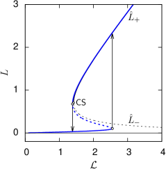
Figure 2: Length of the homogeneous cell as a function of $\mathcal{L}$ in the nonregularized case (thin black line) and in the regularized case (thick blue line). The horizontal solid black line shows collapsed solutions in the nonregularized model. The chosen regularization corresponds to $g=h=1$, $L_{f}=0.1$, and $\alpha=2$. Parameter: $\mathcal{P}/\mathcal{K}=0.5$.

Note that all these sigmoidal dependencies belong to the class of Hill-Langmuir equations with the coefficients $\alpha$, $\beta$, and $\gamma$ usually quantifying the degree of cooperativity. They must be non-negative and sufficiently large to prevent the collapse of a cell. More precisely, since the cell length can be found from the dimensionless algebraic equation $\mathcal{P}h(L)g(L)=-L\mathcal{K}[L-\mathcal{L}f(L)]$, we can conclude that for $L$ much larger than any of the regularizing lengths, the solution coincides with Eq. (20), but for sufficiently small $L$ and $\alpha+\beta+\gamma>1$ there will be another branch $\hat{L}=(\mathcal{K}\mathcal{L}/\mathcal{P})(L_{f}^{\alpha}L_{g}^{\beta}L_{h}^{\gamma})^{1/\nu}$, where $\nu=\alpha+\beta+\gamma-1$. The associated velocity, stress, and motor concentration can then be found from the relations $\hat{\sigma}=\mathcal{K}L\left(L_{f}/L_{r}\right)^{\alpha}$, $\hat{v}=0$ and $\hat{c}=L_{r}^{\gamma-1}/L_{h}^{\gamma}$.

An example of the coexistence of the two branches is presented in Fig. 2 (thick blue line). As we see, the collapse of the cell induced by squeezing takes place discontinuously near the critical value of $\mathcal{L}$ given by Eq. (21). Interestingly, the regularized theory also predicts an inverse transition from collapsed to noncollapsed state when $\mathcal{L}$ increases. The ensuing hysteresis is reminiscent of what happens in the three-dimensional theory of cytokinesis Turlier et al. (2014), which suggests that a possible interpretation of the collapsed states could be associated with cell division. The ambiguity, however, remains since our prototypical model cannot really distinguish between various modalities of the abrupt loss of cell integrity; in particular, it can confuse cell death with cell division. Moreover, the one-dimensional model cannot really differentiate a change of cell volume from a change of cell shape. So, it is not clear that collapsed solutions should be interpreted as cells which fully lose their volume. They rather indicate that the cell cortex undergoes a drastic singularity involved, for instance, in a transition from a squamous to columnar state Hannezo et al. (2014).

Inhomogeneous steady states. Nonsingular solutions of Eqs. (18) can be of motile or static type depending on the symmetry of the motor distribution [see Eq. (16)]. The stability analysis presented in Sec. IV suggests that the only stable inhomogeneous solutions are nonsymmetric motile states with myosin motors localized at the trailing edge; in view of the reflectional symmetry of the problem such solutions appear in pairs. Below we show that an asymptotic representation of such motile solutions can be computed analytically in the double limit $\mathcal{P}\rightarrow\infty$ and $\mathcal{K}\rightarrow\infty$ with the ratio $r=\mathcal{P}/\mathcal{K}$ remaining finite.

Suppose that one of the twin configurations $c(y)$, solving Eqs. (18), has a maximum at $y=0$ and decays to zero away from this point. Then the asymptotic representation of the solution can be written in the form (see Appendix B)

$$c(y)=\frac{\mathcal{P}}{2\cosh^{2}(\mathcal{P}Ly/2)},$$ (23)

where $L$ solves the algebraic equation

$$(\mathcal{P}/2)\coth(L/2)=-\mathcal{K}(L-\mathcal{L}).$$ (24)

The obtained result shows that the motors distribution becomes infinitely localized in the limit $\mathcal{P}\rightarrow\infty$. If we also assume that $\mathcal{P}\sim r\mathcal{K}$ where $r$ is finite we obtain that Eq. (24) has solutions if and only if

$$(r/2)\sqrt{4/r+1}\leq\mathcal{L}-2\sinh^{-1}(\sqrt{r}/2).$$ (25)

Inequality (25) represents the collapse condition and, from Eq. (24), we see that the collapse of a motile cell takes place at finite length $L=2\sinh^{-1}(\sqrt{r}/2)$. In the limit $\mathcal{L}r\ll 1$, condition (25) takes a particularly simple form

$$\mathcal{P}\leq\mathcal{K}\mathcal{L}^{2}/4.$$ (26)

Observe that Eq. (26) coincides with Eq. (21), which suggests that the inhomogeneity of motor concentration affects only weakly the onset of the transition from regular to singular regimes.

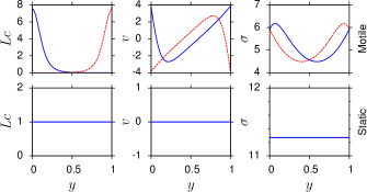
Figure 3: Solution profiles for $\mathcal{P}=10$ and two values of $\mathcal{L}$. The motile solutions correspond to $\mathcal{L}=2$ and the homogeneous stable static state to $\mathcal{L}=1$. For the motile solutions, whether the cell velocity is positive (motors are localized near the boundary $y=0$, solid blue curve) or negative (motors are localized near the boundary $y=1$, dashed red curve) depends on the initial noise $\zeta$; however, both configurations are equiprobable; $V\approx\pm 3.86$, $L\approx 1.94$. Parameter: $\mathcal{K}=100$.

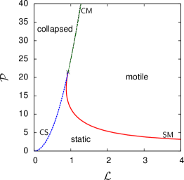
Figure 4: Typical phase diagram in the parameter plane $(\mathcal{L},\mathcal{P})$, where $\mathcal{L}$ is the homeostatic length, which can be interpreted as a scaled stress, and $\mathcal{P}$ is the dimensionless measure of the myosin contractility. The three reachable configurations are motile (M), static (S), and collapsed (C), given the initial data indicated in the text. The dashed blue and solid red lines correspond to CS and SM thresholds, respectively. The black dashed line, essentially overlapping with the green dash-dotted line, indicates the approximation of the CM threshold given by Eq. (26). Parameter: $\mathcal{K}=100$.

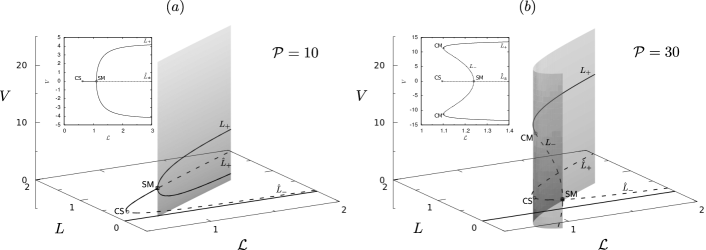
Figure 5: Typical bifurcation diagrams with the homeostatic length $\mathcal{L}$ chosen as a parameter: (a) below the critical end point $\mathcal{P}=10<\mathcal{P}_{*}$ and (b) above the critical end point $\mathcal{P}=30>\mathcal{P}_{*}$. Solution branches representing stable attractors in the initial value problem [Eqs. (14) and (15)] are shown by solid lines; locally unstable solutions are presented by dotted lines. Insets represent projections of the three-dimensional diagram on the $(\mathcal{L},V)$ parameter plane. Parameter: $\mathcal{K}=100$.

IV Phase diagram

To identify stable traveling wave solutions we solved numerically a set of initial value problems for the original nonsteady system of Eqs. (14) and (15). We fixed parameter $\mathcal{K}$, whose effect on the behavior of the system has been studied earlier Recho et al. (2015), and focused on the parameter space $(\mathcal{L},\mathcal{P})$. As initial data we used $L_{i}=\mathcal{L}$ and $c_{i}(y)=1/\mathcal{L}+\zeta(y)$ where $\zeta$ is a random perturbation with zero average. We integrated Eqs. (14) and (15) numerically, analysing transients as the system approached one of the steady states (see Recho et al. (2015) for the method).

The outcomes of our numerical experiments fell into three categories: (i) convergence to a motile solution with motors localized at the trailing edge (M, top row in Fig. 3); (ii) convergence to a homogeneous static solution of the $\hat{L}_{+}$ type (S, bottom row in Fig. 3); and (iii) collapsing solution approaching a singular state C in a finite time. The stability domains of these three “phases” within the $(\mathcal{L},\mathcal{P})$-plane are shown in Fig. 4.

Stability thresholds. The motile (M), static (S), and collapsed (C) regimes are separated by three boundaries which meet at a triple point (symbol $*$ in Fig. 4): the line CS separates collapsed and static ($\hat{L}_{+}$) solutions, the line SM separates static and motile solutions, and the line CM separates collapsed and motile solutions.

The CS line is captured by condition (21) because beyond this line static homogeneous solutions cease to exist. The change of the regime here is abrupt and can be interpreted as a first order transition.

The SM line can be also described analytically if we linearize Eqs. (14) and (15) around the homogeneous solution $\hat{L}_{+}$ and study the limits of linear stability of the homogeneous solution. A standard analysis (Recho et al., 2013, 2015) gives the instability condition $\tanh\left(\omega/2\right)\hat{L}_{+}=\mathcal{P}\omega/2$, where $\omega=(\hat{L}_{+}^{2}-\mathcal{P}\hat{L}_{+})^{1/2}$. The bifurcation is of pitchfork type and can be interpreted as a second order phase transition. Note that a mild generalization of the model accounting for the saturation of contractility as a function of the motor concentration turns the supercritical bifurcation into a subcritical bifurcation Recho et al. (2015).

The CM line, separating motile and collapsed states and corresponding to another first order transition, cannot be expressed analytically. However, at large values of $\mathcal{P}$ and $\mathcal{K}$ such that $\mathcal{K}\mathcal{L}/\mathcal{P}\ll 1$, this transition is asymptotically captured by condition (25). For the realistic parameters used in Fig. 4, expression (25) provides a remarkably good approximation for the CM line starting already at the triple point.

The coordinates of the triple point $(\mathcal{L}_{*},\mathcal{P}_{*})$, which in view of the nature of the SM, CM, and CS transitions should be rather called the “critical end point,” can be found as the intersection of the CS and SM lines. Therefore, $\mathcal{P}_{*}=\mathcal{K}\mathcal{L}_{*}^{2}/4,$ where $\mathcal{L}^{*}$ satisfies the equation $2\tanh(\omega_{*}/2)=\mathcal{K}\omega_{*}\mathcal{L}_{*}^{2}/4$ with $\omega_{*}^{2}=\mathcal{L}_{*}^{2}(\mathcal{K}\mathcal{L}_{*}^{2}-2)/8$.

Bifurcation patterns. To understand better the relation between different types of traveling wave solutions in this problem, we used a numerical continuation method Doedel et al. (1991) with parameter $\mathcal{L}$ varying around the critical end point. We found that, in full agreement with the analysis above, the bifurcation diagrams can be of two types depending on the value of the parameter $\mathcal{P}$ (see Fig. 5).

At $\mathcal{P}<\mathcal{P}_{*}$ the motile solution bifurcates from the homogeneous solution $\hat{L}_{+}$ through a supercritical pitchfork, which we interpret as a continuous phase transition at a critical value of the parameter $\mathcal{L}$ given by the instability condition. We recall that the locus of these points in the parameter space $(\mathcal{L},\mathcal{P})$ is represented in Fig. 4 by the solid red line, SM.

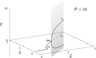
Figure 6: An example of a bifurcation diagram for the regularized model with $g=h=1$, $L_{f}=0.1$, and $\alpha=2$. Parameters: $\mathcal{P}=10$ and $\mathcal{K}=100$.

While the degenerate collapsed solutions are not reachable by the continuation method, we also show in Fig. 5 the collapsed solutions with zero length. Observe that those are the only possible solutions if the parameter $\mathcal{L}$ is below the turning point CS. The locus of the turning points CS is shown in Fig. 4 by a dashed blue line given by Eq. (21).

The collapsed solutions are more adequately represented by the regularized models discussed in Sec. III. In Fig.  6 we show a regularization-induced modification of the bifurcation diagram presented in Fig. 5(a) for the system (14) with $g(L)=h(L)=1$ and $f(L)\neq 1$. A comparison of Figs. 6 and 5(a) shows that regularization did not affect significantly the bifurcation from static to motile solutions even though now there is a finite coexistence domain between collapsed and noncollapsed static solutions (illustrated in more detail in Fig.  2).

Returning to the original, nonregularized setting, we now consider the second type of behavior of the system corresponding to the range $\mathcal{P}>\mathcal{P}_{*}$, where the motile solutions bifurcate from the unstable branch of the homogeneous static solutions $\hat{L}_{-}$. Along the bifurcated motile branch, there is now a turning point CM where the stability of the motile regimes in the full time-dependent problem, Eqs. (14) and (15), is lost. If $\mathcal{L}$ is decreased beyond this turning point, there are no more nondegenerate stable static solutions and, this is the reason why our numerical experiments showed in this range a discontinuous transition to the collapsed state [see Fig. 5(b)]. The locus of the CM turning points in the parameter space $(\mathcal{L},\mathcal{P})$ is shown in Fig. 4 by a dashed green line.

Sensitivity to initial data. Since our numerical study of the time-dependent problem [Eqs. (14) and (15)] was necessarily limited in scope, the actual basin of attraction of each of our three main regimes (static, motile, and collapsed) was not fully mapped in the space of parameters describing the initial data. We have found, however, that the phase diagram in Fig. 4 is robust with respect to rather general perturbations of the initial concentration field.

The dependence of the results on the choice of the initial length is more sensitive. For instance, choosing the initial length in the range $L_{i}\leq\hat{L}_{-}$ leads to a collapse independently of the value of $\mathcal{P}$ and $\mathcal{L}$. This empirical result can be supported by the observation, that for configurations with homogeneous distribution of myosin, Eq. II, reduces to

$$\dot{L}=-2\mathcal{K}\tanh(L/2)(L-\hat{L}_{-})(L-\hat{L}_{+})/L.$$ (27)

This equation reaffirms that the homogeneous state $\hat{L}_{+}$ is stable with the basin $]\hat{L}_{-},\infty[$, while the state $\hat{L}_{-}$ is unstable and any initial state with $[0,\hat{L}_{-}[$ should unconditionally collapse.

V Discussion

Observe that the active mechanism in our model, whose strength scales with parameter $\mathcal{P}$ defined by Eq. (11), is responsible for two different physical effects.

On the one hand, an increase of $\mathcal{P}$ can lead to a collapse of a homogeneous configuration of a cell. This implies breaking the balance between motor contractility and the effective quasielastic resistance. The transition is discontinuous (first order) even though appropriate regularization of the problem can prevent the formation of a singularity.

On the other hand, an increase of $\mathcal{P}$ can be also responsible for the loss of homogeneity and the emergence of polarity. If the incipient concentration gradients are not suppressed by diffusion, motors localize and the cell starts to move. The threshold of such instability is sensitive to the homeostatic length $\mathcal{L}$, defined by Eq. (13), because the homogenizing effect of diffusion is more potent in a small domain than in a large domain. In contrast to the collapse transition, the motility transition is continuous (second order).

In view of the above, the emergence of the three main configurations—motile, static, and collapsed—becomes natural. At $\mathcal{P}<\mathcal{P}_{*}$ the homogeneous solution $\hat{L}_{+}$ is replaced by a motile solution at sufficiently large value of $\mathcal{L}$ when the diffusion is no longer sufficient to prevent the contraction-induced drift. On the contrary, when $\mathcal{L}$ decreases below sufficiently small value, the homogeneous contraction overcomes the cell elastic resistance which triggers the collapse. In between, there is a finite interval of sufficiently small values of $\mathcal{L}$, where stable static solutions exist. In the $\mathcal{P}>\mathcal{P}_{*}$ range, both the symmetrization and the collapse take place simultaneously at a single threshold. The main conclusion is that stable nontrivial static configurations are delicate and may be achievable only in the presence of stretching force dipoles applied to the cell from the environment.

We now interpret these findings in the context of tissue homeostasis. Cells in tissues are typically subjected to stresses exerted by their neighbors and mediated by adherens junctions Guillot and Lecuit (2013). For instance, when epithelial cells reach confluence, they become caged by their neighbors and the formation of adherens junctions effectively jams the cell monolayer through a process known as contact inhibition Garcia et al. (2015). The tension in such monolayers has been monitored using atomic force microscopy indentation Harris et al. (2014) and, during the initial formation of the monolayer when E-cadherin clusters are formed between the cells that are still polarized, the tension and the surface area of the cells increase indicating a rise of the homeostatic length. After this initial stage, the monolayer tension significantly drops. If we interpret this drop as a decrease of $\mathcal{L}$, the observed cell symmetrization within a monolayer becomes natural. Interestingly, the predicted transition from symmetric to collapsed state at even smaller values of $\mathcal{L}$ has been also observed in monolayers. As explained in Wyatt et al. (2016), local decrease of the tensile stress in a tissue can lead to the increase of tissue density (i.e., smaller homeostatic length), which triggers cell extrusion events. The latter may be associated with our cell collapse (see also Marinari et al. (2012); Eisenhoffer et al. (2012); Gudipaty et al. (2017)).

It is also known that scratch-wound assays and laser ablations Tambe et al. (2011); Weber et al. (2012); Vedula et al. (2013) reduce the compressive stresses by creating an available free space. Our model shows that such a reduction could be sufficient for the spontaneous initiation of motility of the leader cells at the margin of the tissue. This puts the tissue under tension Vincent et al. (2015); Blanch-Mercader et al. (2017) and further increases bulk motility needed to heal the wound. Chemotactic signaling is clearly also necessary for normal wound closure. However, the importance of mechanics is corroborated by the observation that a moderate external cell stretching accelerates wound closure Toume et al. (2017).

The closely related phenomenon of the EMT is of significant interest because of its central role in diseases such as fibrosis and cancer Thiery et al. (2009). It is known that the mechanosensitive activation pathways of EMT involve both exogenous and endogenous stresses supported by the cytoskeleton (see Gjorevski et al. (2012) and references therein). If an external stress is applied to a cell in a tissue, the parameter $\mathcal{L}$ will increase, leading to the mechanical loss of stability of a static configuration. The ensuing F-actin flow is characterized by a polymerization of the F-actin meshwork at the cell front. Such a polymerization reduces the pool of G-actin with which a transcription factor MRTF-A is normally associated. This transcription factor then becomes free to accumulate in the cell nucleus, where it promotes the expression of the genes regulating the disassembly of cell-cell contacts, which ultimately liberates the cell from the entanglement with its neighbors.

While a direct pharmaceutical activation of the Rho pathway, which is known to affect the remodeling of the cytoskeleton, can also trigger the nuclear translocation of MRTF-A, our model suggests that both, internal and external stress creation, can generate alternative mechanical pathways regulating the polarization of cells and controlling in this way the emergence of EMT.

VI Conclusions

Cell motility is affected by externally applied forces. Here we argue that not only the resultant, but also the distribution of applied forces matters, in particular, that cell migration may be sensitive to mechanically balanced force couples with zero resultant. This may sound surprising since such couples can squeeze or stretch the cell but do not impose explicit directionality.

To study the effect of the applied force couples, we employed a one-dimensional model incorporating active myosin contraction and accounting for the induced actin turnover. We showed that a symmetrization and a spontaneous motility arrest of a polarized cell can result from squeezing of a steadily moving cell. Conversely, we showed that, if squeezing is relaxed, a static symmetric cell may get again polarized and start to move. An analytical study of the model revealed the exact amount of mechanical stress needed to polarize a static cell and arrest a moving cell.

The proposed model predicts further that sufficiently strong squeezing can lead to the loss of cell integrity and discontinuous collapse of the cell to (almost) zero length. We argued that possible interpretations of the collapsed states could be associated with cell division or death.

The obtained phase diagram in the space of nondimensional parameters distinguishes between motile, static, and collapsed configurations of the cell. It can be relevant for the study of the EMT and may help to understand the mechanical aspects of CI. For instance, the model suggests that an increased cell tension may lead to cell polarization emulating EMT. Instead, squeezing can be the origin of polarity loss, which is a characteristic feature of the CI phenomenon.

Interestingly, our model reveals that self-induced squeezing associated with the active cortical contraction can lead to symmetrization and cell arrest even in the absence of the confining environment. Another insight is that internal homeostatic pressure, originating from actin turnover, may act quantitatively similar to the externally applied stress as a factor promoting cell polarization and motility.

A shortcoming of our analytically tractable model is that neither static solutions nor regularized collapsed solutions carry a nontrivial F-actin flow. Such flows, however, can be recovered in this framework if we assume that contractility is space dependent and controlled by independent biochemical pathways Turlier et al. (2014). Another weakness of the model is the neglect of protrusive stresses at the leading edge associated with actin polymerization. We also left aside the important question of the interplay between the resultant force and the applied force couple, which will manifest itself in a stress dependence of the force-velocity relations. All these issues require further research.

Despite these limitations, we expect that the transparency of the proposed model will motivate focused experimental investigations of the predicted transitions between different regimes and inspire the development of biomimetic devices imitating the rich mechanical behavior of crawling cells. Indeed, by accounting for the whole spectrum of external loadings, the model bridges cellular and tissue scales, and opens new perspectives in the design of the artificial analogs of collective cellular motility.

Appendix A

We represent a cell by a slab of height $H$ and length $L$, confined to a track of constant width $W$. The slab is modeled as a solution of biopolymers enclosed in a plasmic membrane which adheres to the track.

The free energy of the system, $\mathcal{F}$, is the sum of the surface energy $\mathcal{F}_{s}$ and a confinement energy $\mathcal{F}_{c}$ (see Hannezo et al. (2014)). The surface energy can be written in the form $\mathcal{F}_{s}=2\gamma_{m}(LW+LH+WH)-\gamma_{s}LW$, where $-\gamma_{s}<0$ is the cell-substrate surface tension showing that spreading is energetically favored and $\gamma_{m}>0$ is the conventional surface tension of the free membrane. The confinement energy is assumed to be of entropic nature, accounting for the presence of Gaussian polymers inside the slab. The simplest expression then is $\mathcal{F}_{c}=A(1/H^{2}+1/W^{2}+1/L^{2})$, where $A$ is a rheological coefficient whose value depends on the nature of the polymers de Gennes (1979).

Suppose next that, while the surface area of the cell can change through the addition of lipids to the membrane Kinneret (2011), the cell volume $\Omega$ remains constant, tightly regulated by an active osmotic balance between the cell interior and exterior Jiang and Sun (2013); Hui et al. (2014); McGrail et al. (2015). Using the geometrical constraint $\Omega=LHW$, we then eliminate height $H$ from the expression of the free energy to obtain $\mathcal{F}=-\gamma_{s}LW+2\gamma_{m}(LW+\Omega/W+\Omega/L)+A[(LW/\Omega)^{2}+1/W^{2}+1/L^{2}].$

The internal traction $\tau=-(HW)^{-1}\partial_{L}\mathcal{F}$ takes the form

$$\small\tau=-\frac{\gamma L}{\tilde{L}_{f}^{2}\tilde{L}_{0}}\left\{L\left[1-\left(\frac{\tilde{L}_{f}}{L}\right)^{4}\right]-\tilde{L}_{0}\left[1+\frac{\gamma_{m}}{\gamma}\left(\frac{\tilde{L}_{f}}{L}\right)^{2}\right]\right\},$$ (28)

where $\tilde{L}_{f}=\sqrt{\Omega/W}$, $\tilde{L}_{0}=\gamma\Omega^{2}/(2AW)$, and $\gamma=\gamma_{s}-2\gamma_{m}>0$. In the regime $L\gg H$, describing cell spreading, we can drop the fourth power term in Eq. (28). If we further assume that $L\sim\tilde{L}_{0}$, we obtain Eq. (22) with $\alpha=2$; however, our main conclusions about the effect of regularization will survive even without this assumption.

Appendix B

To obtain the desired asymptotic representations of inhomogeneous solutions of Eqs. (18), it will be convenient to reformulate Eqs. (18) as a nonlinear integral equation. First, by combining Eqs. (18b) and (18c), the motor concentration is expressed in the form

$$c(y)=\frac{1}{L}\frac{e^{\Psi(y)}}{\int_{0}^{1}e^{\Psi(y)}dy},$$ (29)

where $\Psi(y)=\sigma(y)-VLy$. In turn, the stress field is written as

$$\sigma(y)=\mathcal{P}L\int_{0}^{1}\phi(y,z)c(z)dz+\bar{\sigma}\theta(y),$$ (30)

where the stress on the boundary is $\bar{\sigma}=-\mathcal{K}(L-\mathcal{L})$. Introducing the Heaviside function $H(x)$, we express the auxiliary functions in Eq. (30) as

$$\phi(y,z)= \frac{\sinh[L(1-z)]\sinh(Ly)}{\sinh(L)}$$

$$-H(y-z)\sinh[L(y-z)],$$

$$\theta(y)= \frac{\cosh(Ly)[1-\cosh(L)+\sinh(L)]}{\sinh(L)}.$$

Using the boundary conditions, we can now link the cell velocity $V$ and its length $L$ to the concentration field with

$$V =\mathcal{P}L\int_{0}^{1}\alpha(y)c(y)dy,$$ (31a)

$$\bar{\sigma} =\mathcal{P}L\int_{0}^{1}\beta(y)c(y)dy,$$ (31b)

where

$$\alpha(y)=\frac{\sinh[L(1/2-y)]}{2\sinh(L/2)},\;\beta(y)=\frac{\cosh[L(1/2-y)]}{2\sinh(L/2)}.$$

Finally, collecting all these expressions together, we obtain an integral representation for $\Psi(y)$:

$$\Psi(y)=\mathcal{P}L\int_{0}^{1}\left[\phi(y,z)+\theta(z)\beta(z)-Ly\alpha(z)\right]c(z)dz.$$ (32)

Substituting Eq. (32) into Eq. (29) we obtain the desired integral equation for $c(y)$

$$c(y)=\frac{1}{L}\frac{e^{\mathcal{P}L\int_{0}^{1}\left[\phi(y,z)+\theta(z)\beta(z)-Ly\alpha(z)\right]c(z)dz}}{\int_{0}^{1}e^{\mathcal{P}L\int_{0}^{1}\left[\phi(s,z)+\theta(z)\beta(z)-Ls\alpha(z)\right]c(z)dz}ds}.$$

Next, as the main contribution to the integral in Eq. (32) arises from the fast decay of the concentration field in the boundary layer at the rear front, we can use the method of matched asymptotic expansions, e.g., Hinch (1991); Verhulst (2005), to obtain the asymptotic analog of Eq. (32) for $\mathcal{P}\gg 1$. After rescaling the concentration field and writing it as $\tilde{c}(u)=\mathcal{P}^{-1}c(u/\mathcal{P})$, where we introduced the blow-up spatial coordinate $u\in[0,\mathcal{P}]$, we obtain

$$\Psi(u)\simeq L\int_{0}^{\infty}R(u,v)\tilde{c}(v)dv+\text{const},$$ (33)

with the kernel

$$R(u,v)=\left\{\begin{array}[]{lc}\frac{L}{2}(v-2u)&\text{if}\;u\leq v,\\ -\frac{L}{2}v&\text{if}\;u>v.\end{array}\right.$$

Note that the constant in Eq. (33) is irrelevant because it does not affect Eq. (29).

We now reformulate the integral equation (29) in a simpler form

$$\tilde{c}(u)=\frac{e^{L^{2}\Phi(u)}}{L\int_{0}^{\infty}e^{L^{2}\Phi(v)}dv},\;\Phi(u)=\int_{0}^{u}(v-u)\tilde{c}(v)dv.$$ (34)

The remaining parameter $r=\mathcal{P}/\mathcal{K}$ enters these relations indirectly through the cell length $L$ which is still unknown.

Given that $\Phi^{\prime}(u)=-\int_{0}^{u}\tilde{c}(v)dv$ and $\Phi^{\prime\prime}(u)=-\tilde{c}(u)$, we then rewrite Eq. (34) in the form

$$L\Phi^{\prime\prime}(u)\int_{0}^{\infty}e^{L^{2}\Phi(v)}dv+e^{L^{2}\Phi(u)}=0.$$ (35)

Using the boundary conditions $\Phi(0)=\Phi^{\prime}(0)=0$, we integrate Eq. (35) explicitly:

$$-\frac{L^{2}}{2}\left(\Phi^{\prime}(u)\right)^{2}=\frac{e^{L^{2}\Phi(u)}-1}{L\int_{0}^{\infty}e^{L^{2}\Phi(v)}dv}.$$ (36)

Since $\Phi(\infty)=-\infty$ and $\Phi^{\prime}(\infty)=-1/L$, we conclude that $L\int_{0}^{\infty}e^{L^{2}\Phi(v)}dv=2$ and then explicit integration of Eq. (36) gives $\Phi(u)=L^{-2}\cosh^{-2}(Lu/2)$ and

$$c(y)=\frac{\mathcal{P}}{2\cosh^{2}(\mathcal{P}Ly/2)}.$$ (37)

The corresponding velocity and stress distributions can be also written explicitly. If we now combine Eq. (37) with Eq. (31a) we find a simple asymptotic expression for the cell velocity $V=\mathcal{P}/2$. Further substitution of Eq. (37) into Eq. (31b) produces the algebraic equation for the cell length $L$,

$$(\mathcal{P}/2)\coth(L/2)=-\mathcal{K}(L-\mathcal{L}),$$

which was quoted in the main text [see Eq. (24)].

References

- Alberts et al. (2014) B. Alberts, A. Johnson, J. Lewis, D. Morgan, M. Raff, K. Roberts, and P. Walter, Molecular Biology of the Cell, 6th ed. (Taylor & Francis Group, 2014).
- Verkhovsky et al. (1999) A. Verkhovsky, T. Svitkina, and G. Borisy, Curr. Biol. 9, 11 (1999).
- Anderson et al. (1996) K. Anderson, Y.-L. Wang, and J. Small, J. Cell Biol. 134, 1209 (1996).
- Heinemann et al. (2011) F. Heinemann, H. Doschke, and M. Radmacher, Biophys. J. 100, 1420 (2011).
- Schreiber et al. (2010) C. H. Schreiber, M. Stewart, and T. Duke, Proc. Natl Acad. Sci. 107, 9141 (2010).
- Recho and Truskinovsky (2013) P. Recho and L. Truskinovsky, Phys. Rev. E 87, 022720 (2013).
- Friedl and Gilmour (2009) P. Friedl and D. Gilmour, Nat. Rev. Mol. Cell Biol. 10, 445 (2009).
- Hakim and Silberzan (2017) V. Hakim and P. Silberzan, Rep. Prog. Phys. 80, 076601 (2017).
- Camley and Rappel (2017) B. A. Camley and W.-J. Rappel, J. Phys. D: Appl. Phys. 50, 113002 (2017).
- Trepat and Fredberg (2011) X. Trepat and J. Fredberg, Trends Cell Biol. 21, 638 (2011).
- Gov (2011) N. Gov, Nature Mater. 10, 412 (2011).
- Trepat et al. (2009) X. Trepat, M. Wasserman, T. Angelini, E. Millet, D. Weitz, J. Butler, and J. Fredberg, Nature Phys. 5, 426 (2009).
- Gov (2009) N. Gov, HFSP J. 3, 223 (2009).
- Kabla (2012) A. Kabla, J. R. Soc. Interface 9, 3268 (2012).
- Tambe et al. (2011) D. Tambe, C. Corey Hardin, T. Angelini, K. Rajendran, C. Park, X. Serra-Picamal, E. Zhou, M. Zaman, J. Butler, D. Weitz, J. Fredberg, and X. Trepat, Nature Mater. 10, 469 (2011).
- Deforet et al. (2014) M. Deforet, V. Hakim, H. Yevick, G. Duclos, and P. Silberzan, Nat. Commun. 5 (2014).
- Garcia et al. (2015) S. Garcia, E. Hannezo, J. Elgeti, J.-F. Joanny, P. Silberzan, and N. S. Gov, Proc. Natl Acad. Sci. 112, 15314 (2015).
- Stramer and Mayor (2016) B. Stramer and R. Mayor, Nat. Rev. Mol. Cell Biol. 18, 43 (2016).
- Gjorevski et al. (2012) N. Gjorevski, E. Boghaert, and C. M. Nelson, Cancer Microenviron. 5, 29 (2012).
- Zhang and Liu (2008) H. Zhang and K.-K. Liu, J. R. Soc. Interface 5, 671 (2008).
- Gossett et al. (2012) D. R. Gossett, T. Henry, S. A. Lee, Y. Ying, A. G. Lindgren, O. O. Yang, J. Rao, A. T. Clark, and D. Di Carlo, Proc. Natl Acad. Sci. 109, 7630 (2012).
- Watanabe-Nakayama et al. (2011) T. Watanabe-Nakayama, S.-i. Machida, I. Harada, H. Sekiguchi, R. Afrin, and A. Ikai, Biophys. J. 100, 564 (2011).
- Sutton et al. (2017) A. Sutton, T. Shirman, J. V. Timonen, G. T. England, P. Kim, M. Kolle, T. Ferrante, L. D. Zarzar, E. Strong, and J. Aizenberg, Nat. Commun. 8, 14700 (2017).
- Lee et al. (1999) J. Lee, A. Ishihara, G. Oxford, B. Johnson, and K. Jacobson, Nature 400, 382 (1999).
- Vogel and Sheetz (2006) V. Vogel and M. Sheetz, Nat. Rev. Mol. Cell Biol 7, 265 (2006).
- Ao et al. (2015) M. Ao, B. M. Brewer, L. Yang, O. E. F. Coronel, S. W. Hayward, D. J. Webb, and D. Li, Sci. Rep. 5, 8334 (2015).
- Gudipaty et al. (2017) S. Gudipaty, J. Lindblom, P. Loftus, M. Redd, K. Edes, C. Davey, V. Krishnegowda, J. Rosenblatt, et al., Nature 543, 118 (2017).
- Tao and Sun (2015) J. Tao and S. X. Sun, Biophys. J. 109, 1541 (2015).
- Taloni et al. (2015) A. Taloni, E. Kardash, O. U. Salman, L. Truskinovsky, S. Zapperi, and C. A. La Porta, Phys. Rev. Lett. 114, 208101 (2015).
- Goldyn et al. (2009) A. M. Goldyn, B. A. Rioja, J. P. Spatz, C. Ballestrem, and R. Kemkemer, J. Cell Sci. 122, 3644 (2009).
- Franze et al. (2009) K. Franze, J. Gerdelmann, M. Weick, T. Betz, S. Pawlizak, M. Lakadamyali, J. Bayer, K. Rillich, M. Gögler, Y.-B. Lu, et al., Biophys. J. 97, 1883 (2009).
- Morita et al. (2007) T. Morita, T. Mayanagi, and K. Sobue, J. Cell Biol. 179, 1027 (2007).
- Doyle et al. (2009) A. D. Doyle, F. W. Wang, K. Matsumoto, and K. M. Yamada, J. Cell Biol. 184, 481 (2009).
- Maiuri et al. (2012) P. Maiuri, E. Terriac, P. Paul-Gilloteaux, T. Vignaud, K. McNally, J. Onuffer, K. Thorn, P. A. Nguyen, N. Georgoulia, D. Soong, et al., Curr. Biol. 22, R673 (2012).
- Jülicher et al. (2007) F. Jülicher, K. Kruse, J. Prost, and J.-F. Joanny, Phys. Rep. 449, 3 (2007).
- Rubinstein et al. (2009) B. Rubinstein, M. F. Fournier, K. Jacobson, A. B. Verkhovsky, and A. Mogilner, Biophys. J. 97, 1853 (2009).
- Mogilner (2009) A. Mogilner, J. Math. Biol. 58, 105 (2009).
- Shao et al. (2010) D. Shao, W.-J. Rappel, and H. Levine, Phys. Rev. Lett. 105, 108104 (2010).
- Doubrovinski and Kruse (2011) K. Doubrovinski and K. Kruse, Phys. Rev. Lett. 107, 258103 (2011).
- Ziebert et al. (2012) F. Ziebert, S. Swaminathan, and I. S. Aranson, J. R. Soc. Interface 9, 1084 (2012).
- Recho et al. (2013) P. Recho, T. Putelat, and L. Truskinovsky, Phys. Rev. Lett. 111, 108102 (2013).
- Giomi and DeSimone (2014) L. Giomi and A. DeSimone, Phys. Rev. Lett. 112, 147802 (2014).
- Tjhung et al. (2015) E. Tjhung, A. Tiribocchi, D. Marenduzzo, and M. Cates, Nat. Commun. 6, 5420 (2015).
- Banerjee and Marchetti (2011) S. Banerjee and M. Marchetti, EPL (Europhysics Letters) 96, 28003 (2011).
- Le Berre et al. (2013) M. Le Berre, Y.-J. Liu, J. Hu, P. Maiuri, O. Bénichou, R. Voituriez, Y. Chen, and M. Piel, Phys. Rev. Lett. 111, 198101 (2013).
- Comelles et al. (2014) J. Comelles, D. Caballero, R. Voituriez, V. Hortigüela, V. Wollrab, A. L. Godeau, J. Samitier, E. Martínez, and D. Riveline, Biophys. J. 107, 1513 (2014).
- Prentice-Mott et al. (2016) H. V. Prentice-Mott, Y. Meroz, A. Carlson, M. A. Levine, M. W. Davidson, D. Irimia, G. T. Charras, L. Mahadevan, and J. V. Shah, Proc. Natl Acad. Sci. 113, 1267 (2016).
- Barnhart et al. (2010) E. L. Barnhart, G. M. Allen, F. Julicher, and J. A. Theriot, Biophys. J. 98, 933 (2010).
- Heisenberg and Bellaïche (2013) C.-P. Heisenberg and Y. Bellaïche, Cell 153, 948 (2013).
- Recho et al. (2015) P. Recho, T. Putelat, and L. Truskinovsky, J. Mech. Phys. Solids 84, 469 (2015).
- Recho et al. (2017) P. Recho, T. Putelat, and L. Truskinovsky, To be submitted (2017).
- Recho et al. (2016) P. Recho, A. Jerusalem, and A. Goriely, Phys. Rev. E 93, 032410 (2016).
- Ranft et al. (2010) J. Ranft, M. Basan, J. Elgeti, J.-F. Joanny, J. Prost, and F. Jülicher, Proc. Natl Acad. Sci. 107, 20863 (2010).
- Ambrosi and Zanzottera (2016) D. Ambrosi and A. Zanzottera, Physica D 330, 58 (2016).
- Kinneret (2011) K. Kinneret, Eur. Biophys. J 40, 1013 (2011).
- Diz-Muñoz et al. (2013) A. Diz-Muñoz, D. A. Fletcher, and O. D. Weiner, Trends Cell Biol. 23, 47 (2013).
- Guo et al. (2017) M. Guo, A. F. Pegoraro, A. Mao, E. H. Zhou, P. R. Arany, Y. Han, D. T. Burnette, M. H. Jensen, K. E. Kasza, J. R. Moore, F. C. Mackintosh, J. J. Fredberg, D. J. Mooney, J. Lippincott-Schwartz, and D. A. Weitz, Proc. Natl Acad. Sci. 114, E8618 (2017).
- Jilkine and Edelstein-Keshet (2011) A. Jilkine and L. Edelstein-Keshet, PLOS Comp. Bio. 7, 1 (2011).
- Du et al. (2012) X. Du, K. Doubrovinski, and M. Osterfield, Biophys. J. 102, 1738 (2012).
- Loosley and Tang (2012) A. J. Loosley and J. X. Tang, Phys. Rev. E 86 (2012), 10.1103/PhysRevE.86.031908.
- Löber et al. (2015) J. Löber, F. Ziebert, and I. S. Aranson, Sci. Rep. 5, 9172 (2015).
- (62) .
- Carlsson (2011) A. Carlsson, New J. Phys. 13, 073009 (2011).
- Lin et al. (2017) S.-Z. Lin, B. Li, G. Lan, and X.-Q. Feng, Proc. Natl Acad. Sci. 114, 8157 (2017).
- Noll et al. (2017) N. Noll, M. Mani, I. Heemskerk, S. J. Streichan, and B. I. Shraiman, Nat. Phys. 13, 1221 (2017).
- Turlier et al. (2014) H. Turlier, B. Audoly, J. Prost, and J.-F. Joanny, Biophys. J. 106, 114 (2014).
- Hannezo et al. (2014) E. Hannezo, J. Prost, and J.-F. Joanny, Proc. Natl Acad. Sci. 111, 27 (2014).
- Doedel et al. (1991) E. J. Doedel, H. B. Keller, and J. P. Kernevez, Int. J. Bifurcation and Chaos 1, 493 (1991), AUTO 07P available via Internet from http://indy.cs.concordia.ca/auto/.
- Guillot and Lecuit (2013) C. Guillot and T. Lecuit, Science 340, 1185 (2013).
- Harris et al. (2014) A. R. Harris, A. Daeden, and G. T. Charras, J. Cell Sci. 127, 2507 (2014).
- Wyatt et al. (2016) T. Wyatt, B. Baum, and G. Charras, Curr. Opin. Cell Biol. 38, 68 (2016).
- Marinari et al. (2012) E. Marinari, A. Mehonic, S. Curran, J. Gale, T. Duke, and B. Baum, Nature 484, 542 (2012).
- Eisenhoffer et al. (2012) G. T. Eisenhoffer, P. D. Loftus, M. Yoshigi, H. Otsuna, C.-B. Chien, P. A. Morcos, and J. Rosenblatt, Nature 484, 546 (2012).
- Weber et al. (2012) G. F. Weber, M. A. Bjerke, and D. W. DeSimone, Dev. Cell 22, 104 (2012).
- Vedula et al. (2013) S. R. K. Vedula, A. Ravasio, C. T. Lim, and B. Ladoux, Physiology 28, 370 (2013).
- Vincent et al. (2015) R. Vincent, E. Bazellières, C. Pérez-González, M. Uroz, X. Serra-Picamal, and X. Trepat, Phys. Rev. Lett. 115, 248103 (2015).
- Blanch-Mercader et al. (2017) C. Blanch-Mercader, R. Vincent, E. Bazellières, X. Serra-Picamal, X. Trepat, and J. Casademunt, Soft Matter 13, 1235 (2017).
- Toume et al. (2017) S. Toume, A. Gefen, and D. Weihs, Int. Wound J. 14, 698 (2017).
- Thiery et al. (2009) J.-P. Thiery, H. Acloque, R. Y. Huang, and M. A. Nieto, Cell 139, 871 (2009).
- de Gennes (1979) P.-G. de Gennes, “Scaling concepts in polymer physics,” (Cornell University Press, 1979) Chap. 9.
- Jiang and Sun (2013) H. Jiang and S. X. Sun, Biophys. J. 105, 609 (2013).
- Hui et al. (2014) T. Hui, Z. Zhou, J. Qian, Y. Lin, A. Ngan, and H. Gao, Phys. Rev. Lett. 113, 118101 (2014).
- McGrail et al. (2015) D. J. McGrail, K. M. McAndrews, C. P. Brandenburg, N. Ravikumar, Q. M. N. Kieu, and M. R. Dawson, Biophys. J. 109, 1334 (2015).
- Hinch (1991) E. Hinch, Perturbation Methods, Cambridge Texts in Applied Mathematics (Cambridge University Press, 1991).
- Verhulst (2005) F. Verhulst, Methods and Applications of Singular Perturbations: Boundary Layers and Multiple Timescale Dynamics, Texts in Applied Mathematics, Vol. 50 (Springer, New York, 2005).
- Barnhart et al. (2011) E. L. Barnhart, K.-C. Lee, K. Keren, A. Mogilner, and J. A. Theriot, PLoS Biol. 9, e1001059 (2011).