A STATISTICAL COMPARISON BETWEEN PHOTOSPHERIC VECTOR MAGNETOGRAMS
OBTAINED BY SDO/HMI and Hinode/SP

Abstract

Since May 1, 2010, we have been able to study (almost) continuously the vector magnetic field in the Sun, thanks to two space-based observatories: the Solar Dynamics Observatory (SDO) and Hinode. Both are equipped with instruments able to measure the Stokes parameters of Zeeman-induced polarization of photospheric line radiation. But the observation modes, the spectral lines, the spatial, spectral and temporal sampling, and even the inversion codes used to recover magnetic and thermodynamic information from the Stokes profiles are different. We compare the vector magnetic fields derived from observations with the HMI instrument on board SDO, with those observed by the SP instrument on Hinode. We have obtained relationships between components of magnetic vectors in the umbra, penumbra and plage observed in 14 maps of NOAA AR 11084. Importantly, we have transformed SP data into observables comparable to those of HMI, to explore possible influences of the different modes of operation of the two instruments, and the inversion schemes used to infer the magnetic fields. The assumed filling factor (fraction of each pixel containing a Zeeman signature) produces the most significant differences in derived magnetic properties, especially in the plage. The spectral and angular samplings have the next largest effects. We suggest to treat the disambiguation in the same way in the data provided by HMI and SP. That would make the relationship between the vector magnetic field recovered from these data stronger, what would favor the simultaneous or complementary use of both instruments.

1. Introduction

The goal of this paper is to compare statistically the vector magnetic fields retrieved from SDO/HMI (Scherrer et al., 2012; Schou et al., 2012) with those from Hinode-SOT/SP (Tsuneta et al., 2008; Lites et al., 2013). We are not interested in the absolute calibration of the magnetograms, but in the comparison between them. We shall provide a way, based on a statistical analysis, to go from the magnetic field measured by one instrument to the other in a similar way as Berger & Lites (2003) did for the imaging polarimeter on SoHO (MDI, Scherrer et al., 1995) and the slit ground-based Advanced Spectro Polarimeter (Elmore et al., 1992). The present comparison is motivated by and follows a similar methodology of Berger & Lites (2003). We also analyze the influence of the various observing configurations and inversion codes (ICs), henceforth called actors, in the derivation of vector magnetic fields.

In addition to the original data provided by HMI and SP, we have created pseudo-SP (SP data spectrally sampled as HMI does) maps to simulate the actors present in HMI. Our rationale is that SP is an instrument with detailed spectral data and a higher angular resolution, which, being optically stable over the period of an observing run, and being free of significant seeing-induced crosstalk, should yield magnetic fields of a higher quality, serving as a kind of “ground truth” measurement for HMI. In Section 2 we describe the instruments and data we are comparing, how we create the pseudo-SP maps, the methodology used to prepare and compare the data, and the comparisons we have carried on. We also remind the reader of the meaning of the statistical parameters used to support our conclusions.

In Section 3, we discuss the vector magnetic field comparisons. We also explore how that comparison might be affected when the spectral sampling, the spatial sampling, the spectral line, the inversion code and the disambiguation code are different. All our results are based on an statistical analysis made over 14 maps of an active region observed simultaneously by HMI and SP. Finally, in Section 4, we summarize our findings and suggest several improvements that might benefit the simultaneous or complementary use of HMI and SP data. In the Appendix, the interested reader may find detailed statistical tables. Although those tables make the length of this paper longer than expected, we believe they are necessary to support our results.

The main goal of this paper is to encourage the solar community to use HMI and SP data either simultaneously or alternatively if one data set is available in one instrument but not in the other. Nowadays, the synergy between the numerical experiments –including simulations and extrapolations– and the observational data is critical for the advance of our knowledge of the Sun. In that sense, to speak the same language makes the communication between those data products easier. Apparently, the majority of the solar community uses the Cartesian system instead of the Spherical coordinate to express the vector magnetic field, and for that reason we decided to offer our results primarily in the Cartesian coordinates system. Therefore, we have conducted our investigation in the Cartesian on-CCD coordinates system, i.e. $\mathbf{B}=\{B_{x},B_{y},B_{z}\}$, although the most important comparisons have been also made for the spherical on-CCD coordinates system, i.e. $\mathbf{B}=\{|B|,\theta_{B},\phi_{B}\}$. As we will see, using the spherical on-CCD coordinates system has a great advantage to decouple the effect of the field strength and the disambiguation in the computation of the horizontal components of the vector magnetic field.

2. Data analysis

HMI and SP instruments make full-polarimetric observations (i.e., the four Stokes parameters I, Q, U and V) of the solar disk and selected areas in the Sun respectively. Both instruments observe spectral lines formed in the photosphere. The polarization induced by the Zeeman effect (e.g., Jefferies, Lites & Skumanich 1989) allows us to infer the photospheric vector magnetic field, given a suitable model for the radiating layers. These models work with the data in what is collectively called an inversion scheme, or simply an “inversion”.

2.1. Data Selection

HMI provides full polarimetric filtergrams of the full solar disk taken in just six carefully selected spectral positions around the Fe I 6173 Å line. Every $\approx~{}69m\AA$, the line is sampled with spectral filtergram with a bandpass of roughly $70m\AA$ (spectral bandpass tunable over $680m\AA$), and the spatial sampling is $0.5\arcsec\times 0.5\arcsec$. The field of view is the whole Sun. While the total polarimetric cycle takes 135 $s$, the vector magnetograms provided by the official web page have a cadence of 12 minutes, as many images are needed to build up an average to improve the signal-to-noise ratio.

The SP data are full slit spectro-polarimetric data in the Fe I 6301 & 6302 Å lines. The data used here have a spatial sampling of $0.30\arcsec\times 0.32\arcsec$, and the spectral sampling is $21m\AA/px$.

There are several data products available for both instruments. In this investigation, the main comparison is between the vector magnetic field recorded in the HMI hmi.B_720s data and the one saved in the SP Level2 data. Albeit, the main goal of this investigation is to provided to the solar community a comparison between these easy-access data as they are.

The hmi.B_720s data are full-disk Milne-Eddigton inversion results with the magnetic field azimuthal ambiguity resolution applied (Hoeksema et al., 2014). The _720s in the name of the data product refers to the post-observation integration in time of the data to improve the S/N ratio, as we mentioned above.

The Level2 data are selected-area Milne-Eddigton inversion results with the magnetic field azimuthal ambiguity resolution not applied.

In addition to the SP Level2 data, we have also used the Stokes profiles originally observed by SP (Level1). The SP Level2 data provide maps of physical variables – such as the field strength, the inclination and the azimuth of vector magnetic field, line-of-sight velocity, and so on– after the inversion of the Stokes profiles recorded in the SP Level1 data.

We have inverted the original Stokes profiles observed by SP considering a filling factor (FF) equal to 1. Since the data used to obtain the vector magnetic field are the original SP Level1 data, i.e. Fe I 6301 & 6302 Å lines., and we use the inversion code used for the official SP inversions, we refer to this data as SP data inverted with FF equal to 1, or SPFF1.

We have created a new data set from the original SP Level1 data. We have convolved the Stokes profiles observed by SP (Level1) corresponding to Fe I 6302Å with the HMI transmission profiles calculated for that line. The HMI pipeline calculates these instrumental profiles for any pixel in the solar disk, so it takes into account the Doppler shift due to the differential rotation in the solar surface. For each SP map, we have calculated the instrumental profiles for the pixel located at the center of the FoV, and applied them to all pixels in that SP map. We refer to the SP data sampled and filtered as HMI filtergrams are made as S2H (after SP to HMI). The S2H data have the same spatial sampling as the original SP data. They are inverted with the same inversion code as HMI, i.e., VFISV with FF equal to 1. Notice for creating the S2H data we only use 1 of the 2 lines observed by SP, since we use the same instrumental profiles used by HMI, which cover a spectral range equivalent to one spectral line in the SP spectropolarimetric data. We have chosen the line Fe I 6302 Å because its effective Landé factor, $g_{eff}$, is the same as the one of the line used by HMI, being $g_{eff}=2.5$ for these two spectral lines. The code that calculates the instrumental transmission profiles for any spectral line at a point of the solar disk is the same used in the HMI pipeline at JSOC. This code was kindly provided in the IDL version by Dr. S. Couvidat from Stanford University.

The SP slit does not always scan the solar surface with a constant step in the perpendicular direction to the slit (Centeno et al., 2009). In some cases, an interpolation may be necessary to have an equally-spaced scan. However, since the ultimate goal in this paper is the comparison between SP maps (and S2H maps) and HMI maps, the interpolation of SP data to an equally-spaced grid as initial step is unnecessary, since the interpolation what matters is the one that matches the SP maps with HMI maps. Therefore, in this paper we have skipped the interpolation of the SP data to equally-spaced grid, and we have directly interpolated the SP magnetic field maps to the HMI ones. Same strategy has been applied to match the S2H maps with HMI maps. More details about the co-alignment procedure are given in Section 2.2.

Although the databases of HMI and SP offer different data products, we have selected the data detailed above since they are the ones that are more directly comparable. Recently, HMI has started to provide similar full-disk vector magnetic field similar to the ones analyzed in this paper, but with a post-observation integration time of the data of 135 and 90 $s$. A comparison between these new HMI data products and SP data would be interesting. That new comparison with the one presented in this paper would allow us to better understand the role played by the S/N. Doubtless, the influence of this factor in the comparison between different instruments is important. Nevertheless, it currently falls out of the scope of this paper.

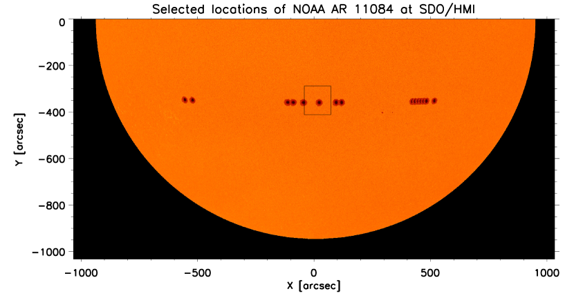
Figure 1.— Locations where NOAA AR 11084 were simultaneously observed by Hinode-SOT/SP and SDO/HMI. The square delimits the size area usually scanned by Hinode-SOT/SP over this AR.

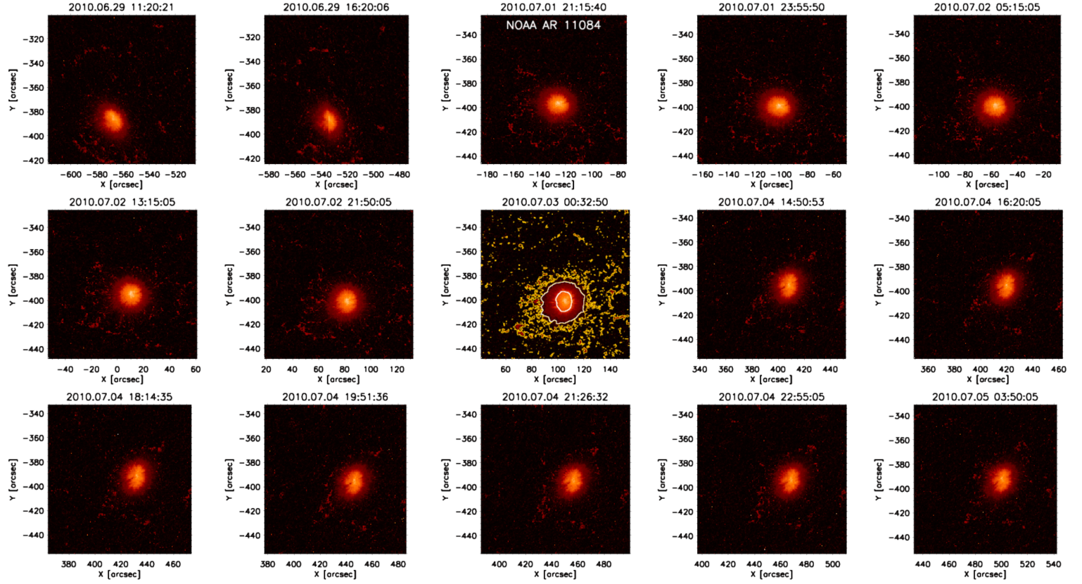
Figure 2.— Magnetic field strength provided by MERLIN IC on NOAA AR 11084 by Hinode-SOT/SP. Contours overplotted on the intensity map observed at 2010.07.03 00:32:50 delimit the umbra-penumbra and the penumbra-moat edges (both in white contours), and the plage (yellow contours). Date and time are relative to the starting time of the scan. Axes are given in heliocentric coordinates.

The SP scans required approximately 30 minutes for this medium size sunspot. In that time, any sunspot may have significantly evolved if undergoing significant activity, e.g., those hosting flare activity or during the initial (non-stationary) emergence phase. Therefore we deliberately selected a mature active region (NOAA AR 11084) with a well-developed sunspot, which is located in a relatively isolated and quiet region. For the comparisons, we selected the HMI data product which was closest in time to the time when the slit of SP was in the middle of its raster. Figure 1 shows the location of NOAA AR 11084 and Fig. 2 shows the magnetic field strength maps provided by the SP Level 2 data as resulting from the Milne-Eddington gRid Linear Inversion Netwrok (hereafter MERLIN) IC on the Level 1 data. Except for the second map in the first row, during which the SP slit jumped, all maps were used. Table 7 in Section 2.1 of the Appendix shows a list with the observational details of the selected data.

In addition to the difference between the instruments used – therefore between the type of data – we have to take into account differences between the ICs used to retrieve the physical information from the data. HMI B_720s series data result from the systematic inversion of observed Stokes filtergrams by the code Very Fast Inversion of Stokes Vector (hereafter VFISV, Borrero & Kobel 2011; Centeno et al. 2014). SP data were inverted by MERLIN. As mentioned above, S2H data were inverted using VFISV as well. Both VFISV and MERLIN are based on the nonlinear least-squares fitting between the synthetic and the observed profiles using the Levenberg-Marquardt algorithm. Both ICs calculate the synthetic Stokes profiles after solving the radiative transfer equation for polarized light under under the Milne-Eddington approximation. Thus, the source function varies linearly with the optical depth, while the other physical parameters are constant through the atmosphere (non-dependence with the optical depth). These codes provide the vector magnetic field, magnetic filling factor, source function and source function gradient, Doppler width, Doppler velocity, damping parameter, and line-to-continuum absorption coefficient.

2.2. Data preparation

In this section, we explain the steps we have applied to the data to make the comparison between them possible. We have applied a semi-automatic alignment method using the routine auto_align_images developed by T. Metcalf, and poly_2d. Both routines and dependent ones are available in the SolarSoftware package. The first step is to identify manually several common structures in both maps. We selected 10 of them. Then, the code matches the maps maximizing the correlation between them applying automatically corrections in shifts in vertical and horizontal direction, rotation and expansion or contraction. We use the output of the first routine as input of poly_2d on the HMI data. All the comparisons between HMI and SP, and HMI and S2H have been made considering the corrections provided by this method.

Even when we have done our best in the alignment between the maps, some misalignment may be present in some cases. Several reasons may cause this misalignment. The hardest one to treat is the a non-constant spatial interpolation between the FoV observed by HMI and SP. That may be produced by a non-constant spatial sampling in the direction perpendicular to the slit, i.e. the size step of the raster changed during the scan, as it has been reported by Centeno et al. (2009). Of course, other reason is the natural evolution of the solar features while the data were taken. As a visual effect, we are able to align very good one side of the FoV, but not so good the other side, where a “stretching” effect may be observed. In the first case, a constant spatial interpolation in the SP data would help to have these data in a more appropriate spatial grid. However, we will need another interpolation to match the HMI spatial scale. We have skipped the first step, and we have to interpolate the SP data directly to HMI. For that reason, we selected 10 points homogeneously distributed in the FoV to warranty the best possible match between the maps. The best alignment achieved is under pixel sampling, i.e., under HMI spatial scale or $\sim 0\arcsec.5$.” During the remapping process the data are interpolated using several procedures.

For SP data, the disambiguation of the azimuth was made using AZAM code. This code was developed by Dr. P. Seagraves and Dr. B. Lites, and it is available in the SolarSoftware distribution. For HMI and S2H data we have used the disambiguation solution map provided with the original HMI data (Hoeksema et al., 2014). While the main results presented in this paper are using AZAM, we have done a detailed studied of the effect introduced by the disambiguation. Thus, we have used three disambiguation solutions. Two are as a result of applying AZAM in slightly different ways. The third is AMBIG, an automatic disambiguation code developed by (Leka et al., 2009a). The core of this code is similar to the one used by HMI, although the setup parameters are slightly different. All in all, there is no significant difference between the three disambiguation results yielded in the comparison HMI $vs$ SP and the ones obtained in the comparison HMI $vs$ S2H (see Table 17 and discussion in Section D). However, if we do not consider those solar features showing opposite sign in the horizontal components – mainly located in the plage –, then the correlation between these data is better. A detailed discussion is presented in section D of the Appendix.

After the co-aligment and the the disambiguation of the azimuth, we calculate the three components of the vector magnetic field in the observer frame, i.e., as it is observed from the Earth.

In our study, we have selected 4 different regions of interest (RoI): umbra, penumbra, strong plage, and weak plage. The umbra and penumbra are calculated taking into account photometric thresholds with respect to the mean value of the continuum Intensity in the local quiet sun ($\tilde{I}_{c,lqs}$). Thus, the umbra is defined as the region where the $I_{c,lqs}<\tilde{I}_{c,lqs}\times 0.55$, while the penumbra is where $\tilde{I}_{c,lqs}\times 0.55<I_{c,lqs}<\tilde{I}_{c,lqs}\times 0.95$. For the plage we have used total polarization slit-reconstructed map from the SP data. We have considered as plage as those locations outside of the umbra and penumbra where the total polarization signal is larger than 0.005. We have split the plage region into strong plage and weak plage considering the values of the components of the vector magnetic field (in Cartesian coordinates, see Section 3.1) or the field strength (in spherical coordinates. The contours of the umbra, penumbra and plage are showed in the central image of fig. 2. Table 1 shows the averaged (in time) values of the minimum, maximum and mean of the magnetic field strength in the RoIs considered in the comparison between $\mathbf{B^{\mathbf{HMI}}_{\mathbf{}}}$  and $\mathbf{B^{\mathbf{SP}}_{\mathbf{}}}$  in spherical coordinates.

Table 1Averaged (in time) values of the minimum, the spatial mean, and the maximum of the magetic field strength in the RoIs of NOAA AR 11084 observed by HMI and SP. Values are given in $G$.

$\mathbf{SolarFeature}$		$\mathbf{<|B|^{HMI}_{min}>}$	$\mathbf{<|B|^{SP}_{min}>}$		$\mathbf{<|B|^{HMI}_{mean}>}$	$\mathbf{<|B|^{SP}_{mean}>}$		$\mathbf{<|B|^{HMI}_{max}>}$	$\mathbf{<|B|^{SP}_{max}>}$
Umbra		$1723\pm 234$	$1881\pm 155$		$2384\pm 75$	$2528\pm 63$		$3006\pm 141$	$3225\pm 123$
Penumbra		$162\pm 90$	$151\pm 81$		$1106\pm 34$	$1177\pm 24$		$2391\pm 61$	$2484\pm 45$
Strong B Plage		$33\pm 8$	$47\pm 19$		$225\pm 14$	$534\pm 22$		$864\pm 67$	$1773\pm 60$
Weak B Plage		$31\pm 8$	$21\pm 9$		$133\pm 6$	$423\pm 46$		$433\pm 80$	$2208\pm 854$

2.3. Data treatement and Inversions Setup

As well as re-binning and filtering SP data to match those of HMI, we must perform what we call cross inversions using the same IC with the different kinds of data or different IC with different data. Table 2 lists the various combinations we have examined. In the following description of the comparison we have made, the expression ‘Original Inverted Data’ refers to use the original inversion results provided by the HMI and SP project official web pages. We have re-binned and interpolated the ‘Original inverted data’ to make possible the spatial matching between them. The comparisons made include:

• Case A: Comparison between Original Inverted Data (HMI $vs$ SP). The straightforward comparison between HMI ( hmi.B_720s) and SP (Level2) is done from the data accessible at the corresponding data base. In this case, we are comparing different data inverted with different inversion code in the two different spectral ranges ( Fe I 6173 Å for HMI, and Fe I 6301 and 6302 Å for SP), and with different filling-factor conditions (FF = 1 for HMI, FF variable for SP). This is the comparison of the data as they are publicly available.

• Case B: Comparison between Original data with different FF (HMI $vs$ SPFF1). In this case, we have modified MERLIN code to use FF=1 on SP data (SPFF1), instead of the data publicly offered, which have FF variable (SP). Both inversions are mode on Fe I 6301 and 6302 ÅṪhis modification of MERLIN was kindly made by Dr. A. de Wijn in CSAC at HAO.

• Case C: Comparison between data equally sampled spectrally (HMI $vs$ S2H). We use VFISV code with FF variable to invert the S2H data. The stray light profile is calculated using the same methodology used by the SP data pipeline. Then, it is convolved with the same HMI instrumental profiles we applied to the corresponding data. From this comparison we infer the influence of the different spectral sampling between the original SP and HMI data.

• Case D: Comparison between data equally sampled with FF fixed to 1 (HMI $vs$ S2HFF1). In this case, we use VFISV code with FF=1 to invert the S2H data (S2HFF1). (By default original HMI data are inverted with the fixed FF to 1.)

• Case E: Comparison between SP data using different FF ( (SPFF1 $vs$ SP).). We use the original SP Stokes profiles data (Level1), and we invert them with MERLIN using different FF, i.e. either with FF variable (SP) or with fixed to 1 (SPFF1). Therefore, we see the influence of the FF during the inversion on the original SP data. In this comparison, we invert both lines Fe I 6301 Åand 6302 Å, as MERLIN does for the original SP data.

• Case F: Comparison between S2H data inverted with FF fixed to 1 and the same data inverted with FF variable (S2HFF1 $vs$ SH2). In this case, we investigate the effect of different FF during the inversion on the S2H data. The data have the same spatial resolution, the observed line is the same (Fe I 6302Å), and the IC used is the same (VFISV).

• Case G: Comparison between S2H and SP data using FF variable (S2H $vs$ SP). In this case, the data have the same spatial and temporal resolution, and are perfectly co-aligned. SP observes Fe I 6301 & 6302 Å spectral lines, while S2H data only considers Fe I 6302 Å. We use different spectral sampling and different ICs.

• Case H: Comparison between S2H and SP data using FF fixed to 1 (SH2FF1 $vs$ SPFF1). Same than case G but using FF fixed to 1,

Table 2Cross inversions setups. The checkmark means coincidence in the value used for both data set. The cross indicates different value used between both instruments. We use ‘$1/2$’ to explicitly mean the number spectral lines used by the inversion code for S2H (Fe I 6302Å) and SP (Fe I 6301 & 6302Å) data. The bullet ($\bullet$) means a filling factor fixed to 1 used during the inversion of data A ($1^{st}$ symbol) or B ($2^{nd}$ symbol) - while the dot inside circle ($\odot$) means a filling factor variable. See section 2.3 for a detailed description.

Case	Data A vs Data B	Spectral Sampling	Spatial Sampling	Spectral Line	Inversion Code	Disambiguation Code	Filling Factor
A	HMI/SP	$\times$	$\times$	$\times$	$\times$	$\times$	$\bullet\odot$
B	HMI/SP	$\times$	$\times$	$\times$	$\times$	$\times$	$\bullet\bullet$
C	HMI/S2H	$\checkmark$	$\times$	$\times$	$\checkmark$	$\checkmark$	$\bullet\odot$
D	HMI/S2H	$\checkmark$	$\times$	$\times$	$\checkmark$	$\checkmark$	$\bullet\bullet$
E	SP/SP	$\checkmark$	$\checkmark$	$\checkmark$	$\checkmark$	$\checkmark$	$\bullet\odot$
F	S2H/S2H	$\checkmark$	$\checkmark$	$\checkmark$	$\checkmark$	$\checkmark$	$\bullet\odot$
G	S2H/SP	$\times$	$\checkmark$	$1/2$	$\times$	$\times$	$\bullet\odot$
H	S2H/SP	$\times$	$\checkmark$	$1/2$	$\times$	$\times$	$\bullet\bullet$

We have intentionally left the impact introduced by the disambiguation solution as the last step of our comparisons. While all the others actors play a significant role in the process of calculation of the field strength, inclination and azimuth of the vector magnetic field, the disambiguation solution will play a different role in the composition of that vector. This is the only case where the information is not contained in the data themselves, we must add information to obtain an “optimal” disambiguated solution (Hoeksema et al., 2014). As we shall show, the chosen solution to the disambiguation problem may have a relevant impact in the correlation between the magnetic field observed by the two instruments. That relationship might be easily improved if both data set solved the disambiguation problem with the same code. A detailed discussion on this topic is given in Section D of the Appendix.

2.4. Comparison of the Data: Statistical Analysis

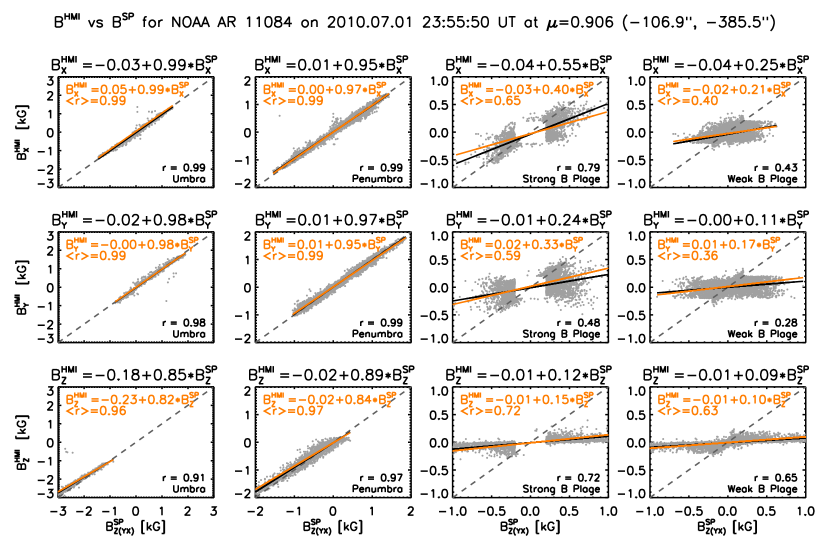
Figure 3.— Scatter plot between the Cartesian components of the vector magnetic field of $\mathbf{B^{\mathbf{HMI}}_{\mathbf{}}}$  and $\mathbf{B^{\mathbf{SP}}_{\mathbf{}}}$ . The linear regression fits and the correlation coefficients for the scatter plots of this particular map are indicated in black. The averaged linear regression fits and correlation coefficients for all the maps are given in orange.

Figure 3 shows the scatter plots for the components of the vector magnetic field $\mathbf{B^{\mathbf{HMI}}_{\mathbf{}}}$  versus $\mathbf{B^{\mathbf{SP}}_{\mathbf{}}}$  at the RoIs, i.e. the comparison between the HMI and SP data as they are provided by the respective official data centers (case A). They show a linear dependency. Hence, we have evaluated a linear regression fit between the components of the vectors $\mathbf{B^{\mathbf{HMI}}_{\mathbf{}}}$  and $\mathbf{B^{\mathbf{SP}}_{\mathbf{}}}$  for the RoIs at each of the 14 selected maps. Tables 8 and 9 in Section B of the Appendix list all the parameters calculated for the comparison between $\mathbf{B^{\mathbf{HMI}}_{\mathbf{}}}$  and $\mathbf{B^{\mathbf{SP}}_{\mathbf{}}}$ . For these linear regression fits we obtain the following parameters: intercept $a$, slope $b$, (estimated) standard deviation of the residuals $s_{e}$, correlation coefficient $r$, and coefficient of determination $r^{2}$. The interpretation of these parameters in this paper is strictly referred to a simple linear regression calculated using the least squares method. Finally, we have calculated averages of intercepts and slopes, averages of the estimated standard deviation ${<}s_{e}{>}\$, correlation coefficients ${<}r{>}\$, and coefficients r-squared ${<}r^{2}{>}\$over the linear regression fits of the all 14 maps analyzed in this paper. The errors of these averages are the standard deviation to their means.

$s_{e}$, is a measure of the typical residual from the least squares line. It is given in the same units of the dependent variable of the linear regression (kG). The correlation coefficients $r$ tell us how well the data fit into a linear regression, i.e. $r$ is a measure of the extent to which the independent and the dependent variable are linearly related. A linear regression is considered showing a strong linear relationship when $1{<}|r|{<}0.8$, a moderate linear relationship when $0.8{<}|r|{<}0.5$, and a weak or negligble relationship when $0.5{<}|r|{\leq}0$. $r^{2}$ may be interpreted as how much the data are spread with respect to the linear fit: High $r^{2}$ represents a small spread, and vice versa. A linear regression fit with a low $r^{2}$ implies a large range of values of one variable (e.g. $B^{HMI}_{Y}$) for a given value of the other variable (e.g. $B^{SP}_{X}$). $r^{2}$ also tells us how much of the variability of one variable can be explained by its (linear) relationship with the other. Therefore, $r^{2}$ is also the fraction of variation that is shared between these variable. For instance, if $r^{2}$ = 0.75, it is said that a 75% of the total variance of the Y variable ($B^{HMI}_{X}$ in our example) is explained by the independent variable ($B^{SP}_{X}$) with the corresponding linear regression fit.

In summary, the average values of $s_{e}$, $r$ and $r^{2}$ analyzed in this article tell us, in a statistical sense, about the error of the estimate, the goodness of the linear relationship, and the percentage of the variation explained of the compared, fitted data using a linear regression fit.

3. Results

In section 3.1, we give the averaged values of the linear regression fit between the components of $\mathbf{B^{\mathbf{HMI}}_{\mathbf{}}}$  and $\mathbf{B^{\mathbf{SP}}_{\mathbf{}}}$  as they are (case A). That section is based on the data released by the respective projects to the public. We investigate the impact of different actors playing a role in the process of recovering the vector magnetic field from the Stokes parameters. We address that investigation through the comparison between the HMI data and the pseudo-SP data (cases B to D), and between SP data and pseudo-SP data (cases F to H) in sections 3.2 and 3.3 respectively. Separately, in section 3.5, we study the relationship between the apparent magnetic flux density and the total flux between for the cases A to D.

In the main body text, we show and explain the statistical values that support our results. Figures and tables showed in the main body text are focused in the comparison between HMI and SP. In the Appendix, we include the statistical tables and other figures related with all the comparisons made in our study.

3.1. Comparison between $\mathbf{B^{\mathbf{HMI}}_{\mathbf{}}}$  and $\mathbf{B^{\mathbf{SP}}_{\mathbf{}}}$ 

We have compared the inversion results available at HMI and SP databases. As we have mentioned before, the disambiguation is the only step not automatically provided with the SP data. For HMI data, this step is easily implemented, since JSOC provides automatically disambiguated inversions. The assumptions behind the algorithm used are summarized in Hoeksema et al. (2014). For the SP maps, we used AZAM code to solve the disambiguation problem (see section D in the Appendix for more details.

Figure 3 shows the linear regression fits between the components of the vector magnetic field of HMI and SP for one individual map (lines and fonts in black). We have over-plotted the averaged linear regression fit over the 14 selected maps (line and fonts in orange). The averaged linear regression fits between the components of $\mathbf{B^{\mathbf{HMI}}_{\mathbf{}}}$  and $\mathbf{B^{\mathbf{SP}}_{\mathbf{}}}$  in each of the RoIs, and the averaged parameters described in the previous section are given in detail in Table 3. They can be interpreted as a translator between the vector magnetic field observed by one instrument to the other. Such data are listed for the RoIs of every map of our data set (see section A).

Table 3Comparison between the Cartesian components of the vector magnetic field observed by HMI and SP. The meaning of the columns is as follows: 1) solar feature or region of interest (RoI); 2) averaged linear regression fit between the variables compared; 3) averaged estimated standard error about the least squares line, ${<}s_{e}{>}$; 4) averaged correlation coefficient, ${<}r{>}$; 5) averaged coefficient of determination, ${<}r^{2}{>}$. The errors in the averaged variables are the standard deviation of the corresponding mean. Values for the magnetic field components are given in $kG$.

$\mathbf{Solar\ Feature}$	$\mathbf{B^{\mathbf{HMI}}_{\mathbf{}}}$  vs $\mathbf{B^{\mathbf{SP}}_{\mathbf{}}}$	$\mathbf{<s_{e}>}$	$\mathbf{<r>}$	$\mathbf{<r^{2}>}$
Umbra	$B^{HMI}_{X}=(+0.05\pm 0.10)+(+0.99\pm 0.02)\times B^{SP}_{X}$	$0.09\pm 0.02$	$0.99\pm 0.00$	$0.99\pm 0.01$
	$B^{HMI}_{Y}=(-0.00\pm 0.04)+(+0.98\pm 0.02)\times B^{SP}_{Y}$	$0.09\pm 0.02$	$0.99\pm 0.00$	$0.98\pm 0.01$
	$B^{HMI}_{Z}=(-0.23\pm 0.10)+(+0.82\pm 0.06)\times B^{SP}_{Z}$	$0.10\pm 0.03$	$0.96\pm 0.02$	$0.93\pm 0.04$
Penumbra	$B^{HMI}_{X}=(+0.00\pm 0.01)+(+0.97\pm 0.02)\times B^{SP}_{X}$	$0.10\pm 0.01$	$0.99\pm 0.00$	$0.98\pm 0.01$
	$B^{HMI}_{Y}=(+0.01\pm 0.01)+(+0.95\pm 0.02)\times B^{SP}_{Y}$	$0.11\pm 0.02$	$0.99\pm 0.00$	$0.97\pm 0.01$
	$B^{HMI}_{Z}=(-0.02\pm 0.01)+(+0.84\pm 0.05)\times B^{SP}_{Z}$	$0.11\pm 0.01$	$0.97\pm 0.01$	$0.94\pm 0.01$
Strong B Plage	$B^{HMI}_{X}=(-0.03\pm 0.01)+(+0.40\pm 0.11)\times B^{SP}_{X}$	$0.16\pm 0.02$	$0.65\pm 0.12$	$0.44\pm 0.14$
	$B^{HMI}_{Y}=(+0.02\pm 0.01)+(+0.33\pm 0.08)\times B^{SP}_{Y}$	$0.16\pm 0.01$	$0.59\pm 0.10$	$0.35\pm 0.12$
	$B^{HMI}_{Z}=(-0.01\pm 0.01)+(+0.15\pm 0.01)\times B^{SP}_{Z}$	$0.07\pm 0.01$	$0.72\pm 0.02$	$0.52\pm 0.04$
Weak B Plage	$B^{HMI}_{X}=(-0.02\pm 0.01)+(+0.21\pm 0.04)\times B^{SP}_{X}$	$0.10\pm 0.01$	$0.40\pm 0.05$	$0.17\pm 0.04$
	$B^{HMI}_{Y}=(+0.01\pm 0.01)+(+0.17\pm 0.04)\times B^{SP}_{Y}$	$0.10\pm 0.00$	$0.36\pm 0.05$	$0.14\pm 0.04$
	$B^{HMI}_{Z}=(-0.01\pm 0.00)+(+0.10\pm 0.02)\times B^{SP}_{Z}$	$0.05\pm 0.00$	$0.63\pm 0.03$	$0.40\pm 0.04$

Table 4Comparison between the spherical components of the vector magnetic field observed by HMI and SP. Magnetic field strength ($|B|$) is given in $kG$. Inclination ($\theta_{B}$) and the azimuth ($\phi_{B}$) of the magnetic field are given in $degree$.

$\mathbf{SolarFeature}$	$\mathbf{B^{\mathbf{HMI}}_{\mathbf{}}}$  vs $\mathbf{B^{\mathbf{SP}}_{\mathbf{}}}$	$\mathbf{<s_{e}>}$	$\mathbf{<r>}$	$\mathbf{<r^{2}>}$
Umbra	$|B|^{HMI}=(-0.11\pm 0.31)+(0.99\pm 0.12)\times|B|^{SP}$	$0.10\pm 0.03$	$0.92\pm 0.05$	$0.84\pm 0.09$
	$\theta_{B}^{HMI}=(12.60\pm 1.89)+(0.91\pm 0.01)\times\theta_{B}^{SP}$	$1.89\pm 0.57$	$0.99\pm 0.01$	$0.98\pm 0.02$
	$\phi_{B}^{HMI}=(14.77\pm 6.60)+(0.82\pm 0.08)\times\phi_{B}^{SP}$	$29.04\pm 5.67$	$0.77\pm 0.12$	$0.61\pm 0.18$
	$\phi_{B}^{HMI\ DIS}=(5.48\pm 10.49)+(0.97\pm 0.05)\times\phi_{B}^{SP\ AZAM}$	$19.11\pm 3.85$	$0.91\pm 0.04$	$0.83\pm 0.08$
Penumbra	$|B|^{HMI}=(0.01\pm 0.01)+(0.93\pm 0.02)\times|B|^{SP}$	$0.13\pm 0.02$	$0.96\pm 0.01$	$0.91\pm 0.02$
	$\theta_{B}^{HMI}=(14.37\pm 2.01)+(0.86\pm 0.02)\times\theta_{B}^{SP}$	$4.98\pm 0.40$	$0.97\pm 0.02$	$0.94\pm 0.03$
	$\phi_{B}^{HMI}=(13.00\pm 4.82)+(0.85\pm 0.04)\times\phi_{B}^{SP}$	$24.95\pm 2.49$	$0.87\pm 0.03$	$0.75\pm 0.05$
	$\phi_{B}^{HMI\ DIS}=(13.11\pm 6.93)+(0.92\pm 0.03)\times\phi_{B}^{SP\ AZAM}$	$36.28\pm 6.33$	$0.92\pm 0.03$	$0.85\pm 0.05$
Strong B Plage	$|B|^{HMI}=(0.19\pm 0.01)+(0.07\pm 0.03)\times|B|^{SP}$	$0.12\pm 0.01$	$0.16\pm 0.08$	$0.03\pm 0.03$
	$\theta_{B}^{HMI}=(56.19\pm 1.83)+(0.39\pm 0.02)\times\theta_{B}^{SP}$	$11.06\pm 0.77$	$0.83\pm 0.01$	$0.68\pm 0.02$
	$\phi_{B}^{HMI}=(52.10\pm 7.52)+(0.43\pm 0.09)\times\phi_{B}^{SP}$	$42.11\pm 2.15$	$0.46\pm 0.06$	$0.21\pm 0.06$
	$\phi_{B}^{HMI\ DIS}=(122.92\pm 7.75)+(0.45\pm 0.03)\times\phi_{B}^{SP\ AZAM}$	$82.86\pm 5.05$	$0.47\pm 0.04$	$0.22\pm 0.04$
Weak B Plage	$|B|^{HMI}=(0.13\pm 0.01)+(0.00\pm 0.01)\times|B|^{SP}$	$0.04\pm 0.00$	$0.01\pm 0.04$	$0.00\pm 0.00$
	$\theta_{B}^{HMI}=(62.72\pm 2.41)+(0.30\pm 0.02)\times\theta_{B}^{SP}$	$11.17\pm 0.97$	$0.78\pm 0.02$	$0.61\pm 0.03$
	$\phi_{B}^{HMI}=(72.95\pm 4.70)+(0.19\pm 0.03)\times\phi_{B}^{SP}$	$44.44\pm 0.88$	$0.20\pm 0.02$	$0.04\pm 0.01$
	$\phi_{B}^{HMI\ DIS}=(174.89\pm 9.38)+(0.23\pm 0.02)\times\phi_{B}^{SP\ AZAM}$	$85.83\pm 2.88$	$0.26\pm 0.02$	$0.07\pm 0.01$

On average, both in the umbra and penumbra the horizontal components of the vector magnetic field ($B_{X}$ and $B_{Y}$, all values are given in kG units) show a slope very close to 1 (${<}b{>}\$$\geq 0.95$), while for the longitudinal component ($B_{Z}$) is smaller ($\sim 0.83\pm 0.05$). In the next sections we will explore this significant discrepancy. The errors in the intercept for the umbra are larger than for the penumbra, especially if we compare them with the errors at the other RoIs ($\leq 0.01$). The ${<}r{>}\$and ${<}r^{2}{>}\$for these RoIs are very close to 1 for the horizontal components and slightly smaller for the vertical component. Therefore, we can say that the values of the components of vector magnetic field $\mathbf{B^{\mathbf{HMI}}_{\mathbf{}}}$  at the umbra and penumbra can be accurately predicted by $\mathbf{B^{\mathbf{SP}}_{\mathbf{}}}$  from the linear relationship showed in the first six rows of Table 3.

In the strong plage, i.e. where 200 G $<(\mid$ $\mathbf{B^{\mathbf{HMI}}_{\mathbf{XYZ}}}$ $\mid$ or $\mid$ $\mathbf{B^{\mathbf{SP}}_{\mathbf{XYZ}}}$ $\mid)<$ 1000 G, the ${<}s_{e}{>}\$is $160$G for the horizontal components and 70 G for the vertical component with correlations ${<}r{>}\$$\sim 0.60$, and $0.72$ respectively. Although the errors of ${<}r{>}\$for the horizontal components are larger, what indicates a large scattering of the $r$ value of the individual comparisons of the horizontal components. The percentage of variation shared by the variables is ${<}r^{2}{>}\$$\sim 50\%$ for the vertical component. For the horizontal components, ${<}r^{2}{>}\$slightly smaller, being $44\%$ and $35\%$ for the X and Y component respectively. The averaged slope ${<}b{>}\$for the horizontal components are between $2$ and $3$ times larger than for the vertical component. Therefore, the components of the vector magnetic field at HMI can be predicted from those at SP and vice versa, with a moderate confidence.

Finally, in the weak plage, i.e. where $(\mid$ $\mathbf{B^{\mathbf{HMI}}_{\mathbf{XYZ}}}$ $\mid$ or $\mid$ $\mathbf{B^{\mathbf{SP}}_{\mathbf{XZY}}}$ $\mid)<200G$, ${<}s_{e}{>}\$for the horizontal components is $\sim 100$G and $\sim 50G$ for the vertical. The ${<}r{>}\$for the horizontal components shows only a weak linear relationship, while for the vertical component the linear relationship is moderate. Only around $15\%$ of the variation of $\mathbf{B^{\mathbf{HMI}}_{\mathbf{XY}}}$  may be explained from $\mathbf{B^{\mathbf{SP}}_{\mathbf{XY}}}$ , and $40\%$ for the vertical component. The errors in all the averaged statistical variables for the weak plage are small. That means, the scattering of the individual statistical variables is small: there is a trend in these variables. On average, the behavior in the weak plage, having a weak linear correlation, is similar in all the individual maps. We have to be careful with the interpretation of the small values of the errors for the plage. The errors for the weak plage are smaller than for the strong plage. However, the normalized variance, i.e. the standard deviation divided by the average of the field values, is higher in the weak plage than in the strong plage, as one may expect from a poorer S/N in the weak plage –because of the low signal there–, with respect to the S/N in the strong plage –where the signal is higher.

Table 4 compares the components of the vector magnetic field in spherical coordinates. In this case, the weak and strong plage are defined as those pixels of the plage region (pixels outside of the sunspot with $P_{tot}>0.005$) where $(|B|^{HMI}$ or $|B|^{SP})<200G$ and $200<(|B|^{HMI}$ or $|B|^{SP})<1500G$ respectively.

Fig. 4 shows, in the $1^{st}\$and the $2^{nd}\$column respectively, the components of the magnetic field of $\mathbf{B^{\mathbf{HMI}}_{\mathbf{}}}$  and $\mathbf{B^{\mathbf{SP}}_{\mathbf{}}}$  of the maps compared through the scatter plots in Fig. 3. In the top panels, from top to bottom, we show $B_{X},B_{X},B_{Z}$ for the sunspot zoomed in. Similarly, in the bottom panels we show the plage. We have masked the sunspot to emphasize its values. A visual inspection of the maps qualitatively shows the same quantitative results as in Table 3 does. The values in the umbra and penumbra are very similar in the $1^{st}\$and $2^{nd}\$columns. All the components of the vector magnetic field (especially in X and Y) in the region of the plage closer to the sunspot are rather similar between them, but in the outer part they are very different. There is a region, between $30<X(\arcsec)<85$ and $0<Y(\arcsec)<30$, where there are several solar features hosting different sign between the values observed by $\mathbf{B^{\mathbf{HMI}}_{\mathbf{Y}}}$  and $\mathbf{B^{\mathbf{SP}}_{\mathbf{Y}}}$  – two circles point some of them out in the $5^{th}$ row of the figure. These differences are due to the manner in which the disambiguation algorithms work on the diverse kinds of data explored here. In the SP maps, the disambiguation results arise from the noisy Q and U signals which in turn result from low values of the horizontal field components in the plage. This divides those maps in two regions each with a dominant sign. Section D of the Appendix proves that different solutions provided by different disambiguation methods produce statistically similar results to the ones showed in Table 3, that is, in the comparison between the magnetic field for HMI and SP. However, if we would consider those pixels sharing the same sign – that means, there where both disambiguation code yield the same solution–, then the improvement of the correlation between the horizontal components is important (e.g. the variation of $\mathbf{B^{\mathbf{HMI}}_{\mathbf{XY}}}$  explained by $\mathbf{B^{\mathbf{SP}}_{\mathbf{XY}}}$  would increase in about $\sim 35\%$ in the strong plage and $\sim 40\%$ in the weak plage, see Table 18).

Figures 5 and 6 show a comparison of the components of the $\mathbf{B^{\mathbf{HMI}}_{\mathbf{}}}$  and $\mathbf{B^{\mathbf{SP}}_{\mathbf{}}}$  in spherical coordinates for the sunspot and plage respectively. The last row of these figures show the disambiguated azimuth obtained from different methods. A detailed comparison of the solutions for the disambiguation is given in the Appendix. However, at a glance, it is easy to see an important result: the disambiguation method used has an strong effect to determine the vector magnetic field, especially in the plage. Thus, the values of field strength ($|B|$), inclination ($\theta_{B}$), and azimuth ($\phi_{B}$) of the vector magnetic field derived from the data observed by HMI and SP are very similar in the sunspot ($1^{st}\$and $2^{nd}\$column of Fig. 5). However, those values are quite different in the plage. Notice $\mathbf{B^{\mathbf{SP}}_{\mathbf{}}}$  is computed considering FF variable, while $\mathbf{B^{\mathbf{HMI}}_{\mathbf{}}}$  is done with FF equals to 1. Therefore, the components of the vector magnetic field in SP data may show values rather different than the corresponding in HMI data. As we mentioned above, this effect is more notorious in the plage than in the umbra and penumbra, where the FF is close to 1. Thus, in the plage, there are regions where $|B|$ reaches values above 1 $kG$ in the SP data (in light green in the images of the $1^{st}\$row of Fig. 5, and in white in the images of the $1^{st}\$row of Fig. 6). While for those location the values are a few tens in HMI data (in dark violet in those images). For that reason, in the Table 1, the values of $|B|$ in the weak and strong plage in the analyzed SP data are showing a large range and a large dispersion, while the analyzed HMI data show a tighter range and a smaller dispersion. As a consequence of the large difference in these values, the linear relationship between $|B|^{HMI}$ and $|B|^{SP}$ in the plage is close to 0 (see Table 4), and the linear correlation between these values is very weak. However, when we consider $|B|$ with the inclination and azimuth, as we compose the vector magnetic field in the Cartesian coordinates, the relationships between the components in that reference system (see Table 3) show a low relationship but different than 0, and a moderate and a weak linear correlation for the strong and weak plage respectively.

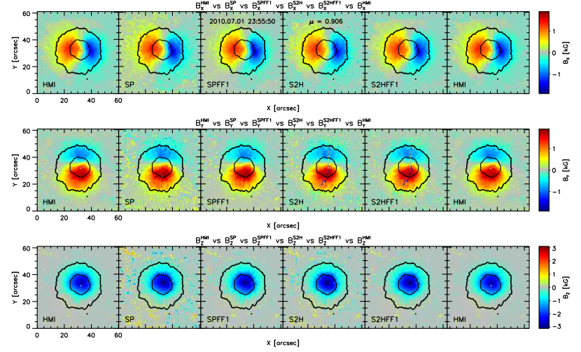
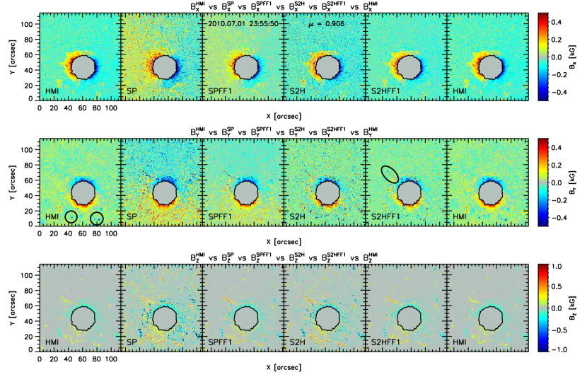
Figure 4.— Components of the vector magnetic field in Cartesian coordinates observed by HMI ($1^{st}\$column), SP ($2^{nd}\$column), SP with FF=1 ($3^{rd}\$column), S2H ($4^{th}$ column), S2H with FF=1 ($5^{th}$ column), and, for making the visual comparison easier to the reader, again HMI ($6^{th}$ column) in the sunspot ($1^{st}\$to $3^{rd}\$row) and the plage ($4^{th}$ to $6^{th}$).

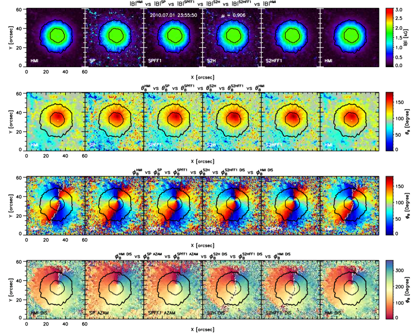
Figure 5.— Components of the vector magnetic field in spherical coordinates observed by HMI ($1^{st}\$column), SP ($2^{nd}\$column), SP with FF=1 ($3^{rd}\$column), S2H ($4^{th}$ column), S2H with FF=1 ($5^{th}$ column), and, for making the visual comparison easier to the reader, again HMI ($6^{th}$ column) in the sunspot ($1^{st}\$to $3^{rd}\$row) and the plage ($4^{th}$ to $6^{th}$).

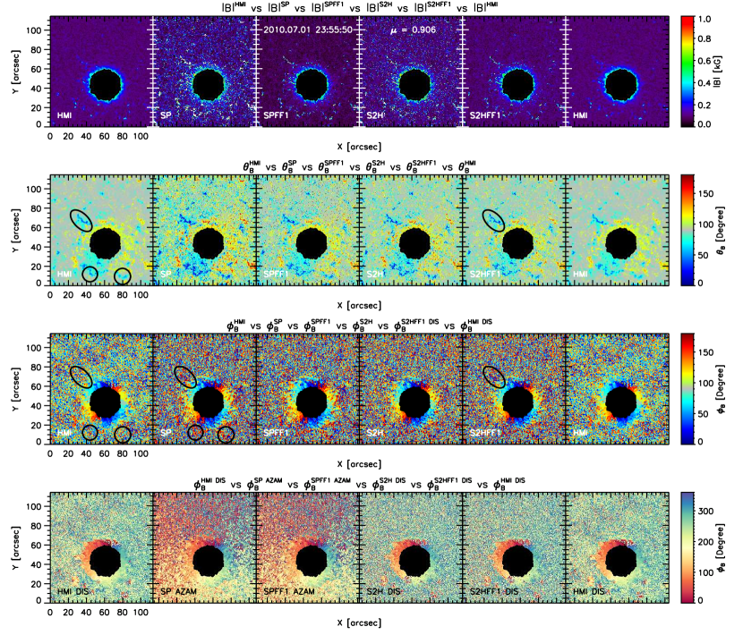
Figure 6.— Components of the vector magnetic field in spsherical coordinates observed by HMI ($1^{st}\$column), SP ($2^{nd}\$column), SP with FF=1 ($3^{rd}\$column), S2H ($4^{th}$ column), S2H with FF=1 ($5^{th}$ column), and, for making the visual comparison easier to the reader, again HMI ($6^{th}$ column) in the sunspot ($1^{st}\$to $3^{rd}\$row) and the plage ($4^{th}$ to $6^{th}$).

3.2. Comparison between HMI and pseudo-SP maps

This section is devoted to understand the role played for those actors which differ between HMI and SP data. They are: the spectral sampling, the spatial sampling, the spectral line, the inversion code, the disambiguation code, and the filling factor.

We call the modified SP maps pseudo-SP maps, and we refer to them as S2H. Table 2 documents the calculated modifications to the original SP data, and Section 2.3 offers details about these comparisons. The complete Table 10 in the Appendix, similar to the one used for the straightforward comparison, supports our findings.

The $3^{rd}$ column in the panels of the Fig. 4 shows the components of the vector magnetic field as result of inverting the SP data with FF=1. The $4^{th}$ shows the S2H data inverted with FF variable, i.e., the SP data are filtered as HMI does, inverted with VFISV and disambiguated as HMI does. The $5^{th}$ column of that figure shows the S2H data inverted similarly but with FF=1. For a better visual comparison, HMI data are displayed again in the last ($6^{th}$) column. Figure 4, and Fig. 10 in the Appendix, visually summarize most of our findings.

Again, values of all the components of the vector magnetic field in the umbra and penumbra are very similar in all the cases. In these RoIs, the FF of the original SP data is variable but is very close to 1, so that the inversions assuming a FF=1 are not largely in error. The signal of the Stokes profiles is much larger than the noise in these regions, therefore, even with a sample of 6 spectral samples – as HMI does–, VFISV is able to reproduce and fit adequately the Stokes profiles, and so to recover the same physical information as inversions using the full spectrum. The richness in the spatial structures of the penumbra may be distinguished in the SPFF1, S2H and S2HFF1 maps. A visual comparison of pseudo-SP maps with the SP original data reveals a penumbra slightly blurrier, but sharper than the equivalent HMI images. Therefore, the spatial information, understood as the physical information by pixel, remains despite of the spectral sampling (S2H maps) or being inverted with FF fixed to 1 (SPFF1 and S2HFF1). The three components of the vector magnetic field of SPFF1 and S2HFF1 are visually closer to the ones observed by HMI than the corresponding to SP and S2H. Therefore the treatment of FF during the inversion seems to be more important than the spectral sampling or the inversion code used. Note that S2H and S2HFF1 data are inverted using VFISV and the same disambiguation solution used by HMI, while SP and SPFF1 data are inverted using MERLIN and a disambiguation solution obtained with AZAM. In the moat – an annular region around the sunspot mainly visible in the magnetograms (Vrabec, 1974) as the place where the moving magnetic features (Harvey & Harvey, 1973) run away from the penumbra as extension of the penumbral filaments (Sainz Dalda & Martínez Pillet, 2005) – the sign of the horizontal components seem to match in all the cases, so the disambiguation has not an apparent effect in that region, as it does not have in the umbra and penumbra either.

Data for the plage are displayed in the bottom panel of Fig. 4. For the SPFF1 maps, we see the same effect in the horizontal components as for the SP data; half of the plage shows a predominant sign, and the other half shows the opposite. It is due to disambiguation solution chosen. Despite this visual effect, this has no impact in the statistical values of the comparison between the vector magnetic field of HMI and SP (see D in the Appendix). For the S2H and SH2FF1 data, as we are using the same disambiguation solution that HMI, the sign of the horizontal component matches with HMI in most of the map. However, the sign in the solar feature located in the circles in the HMI data (colored as blue and mixed blue-red) seems to mach only with the S2H and S2HFF1 maps (blue and mixed colors), but not with the SP and SPFF1 maps (hosting red-colored values). These kind of regions, which were assigned with a different sign by the disambiguation code have an important impact in the correlation of the variables studied, as we have proven in Section D of the Appendix.

Figure 4 allows us to appreciate visually the impact of the FF, the spatial and the spectral sampling, and the disambiguation in the comparison carried out in our study. Thus, HMI maps ($1^{st}\$column) seem to match visually better with maps on the far right: being the worse match with SP ($2^{nd}\$column), the match is a bit better with SPFF1 ($3^{rd}\$column), becoming acceptable with the S2H ($4^{th}$ column), and finally, with the S2HFF1 ( $5^{th}$ column), where the visual match seems to be the best possible.

In the comparison between the spherical components (Figs. 5 and 6), we can appreciate that field strength and inclination of S2HFF1 ($5^{th}$ column) are very similar to the ones of HMI ($6^{th}$ column). Nevertheless, for the azimuth, the pseudo-SP maps are visually closer to SP data than to HMI. This is specially evident in the plage maps (see Fig. 6). We can see the effect introduced by the disambiguation method to calculate the azimuth used to compose the horizontal components of $\mathbf{B^{\mathbf{}}_{\mathbf{}}}$  in the last column of Fig. 6. We can visually distinguish how close the disambiguated S2H azimuth data come to the disambiguated HMI data (both using the same disambiguation method denoted as ’DIS’), and how different the disambiguated SP data are from the HMI DIS. Tables 10 and 15 in the Appendix support these visual impressions for the disambiguation method used in the core of this paper, and others method used to investigate this effect: AZAM2 and AMBIG, see D in the Appendix.

Averaged statistical values in the umbra and penumbra are very similar in all the cases. The slope, ${<}b{>}\$, of the linear regression between vertical component of $\mathbf{B^{\mathbf{HMI}}_{\mathbf{}}}$  and the one of the pseudo-SP maps, shows lower values ($\sim 0.85$ in the umbra, and $\sim 0.90$ in the penumbra) than for the horizontal components ($\sim 0.99$). As noted above, a similar result was found between $\mathbf{B^{\mathbf{HMI}}_{\mathbf{Z}}}$  and $\mathbf{B^{\mathbf{SP}}_{\mathbf{Z}}}$ . Therefore, this behavior must be due to other factor(s) than spectral sampling, filling factor or the combination of both.

In the strong plage, the SPFF1 data can account for $\sim 20\%$ more of the variation of HMI than the basic SP data do. In weak plage, the improvement is $9\%$ for the horizontal components, and $18\%$ for the vertical component. In the case of S2H, where the improvement is only relevant for the X component of the vector magnetic field, $\mathbf{B^{\mathbf{S2H}}_{\mathbf{X}}}$  accounts for $\sim 30\%$ more of the variation of $\mathbf{B^{\mathbf{HMI}}_{\mathbf{X}}}$  than $\mathbf{B^{\mathbf{SP}}_{\mathbf{X}}}$ . This improvement in X alone may be produced by a more accurate sampling of the Stokes Q and/or U profiles than the Stokes V. Again, the averages show that FF has a more important role than the spectral sampling: more variation in $\mathbf{B^{\mathbf{HMI}}_{\mathbf{}}}$  data can be explained with $\mathbf{B^{\mathbf{SPFF1}}_{\mathbf{}}}$  than with $\mathbf{B^{\mathbf{S2H}}_{\mathbf{}}}$ . In plages, a combination of both FF and the spectral sampling improves all the statistical correlations. Values of ${<}r{>}\$for X and Y are $0.92$ and $0.84$ respectively, while for the Y component is very close ($0.72$). The ${<}r{>}\$for the X and Z components are 0.78 and 0.76 respectively. For the Y component, the ${<}r{>}\$is smaller, 0.42. In the strong plage, the X and Z component of S2HFF1 are respectively able to explain $84\%$ and $72\%$ of the variation of HMI, i.e. $40\%$ and $18\%$ more than SP does. For the weak plage, these values are $\sim 60\%$, that means a $43\%$ more for X, and $17\%$ more for Z than for SP. The percentages for Y are sightly slower than the percentages of the case SPFF1, but larger than the ones of the case S2H.

In the Y maps of Fig. 4, we have pointed out some structures with different sign in the SP data with respect to the HMI and S2H maps. A region with a strong signal in the plage is present in all the SP and pseudo-SP maps. However, in HMI these structures cannot be distinguished (colored in light green, grey, and light blue.) That region is pointed out by an ellipse in the Y map of the plage for the case S2HFF1. There, the values are predominantly negative (blue) in the SP and SPFF1 maps, while it is mixed (blue and red) in the S2H and S2HFF1 maps. Thus, the low, mixed values of that region in the HMI map are correlated with values in the SP and SPFF1 maps having a same sign, while for S2H and S2HFF1 maps, the HMI values are correlating with mixed values, therefore, introducing a slight spread in the correlation. That is not the case in the X and Z component, where most of the solar structures seem to share the same sign in all the maps, although they may be more intense in the SP and the pseudo-SP maps than in the HMI ones (e.g., red in the former, yellow in the latter).

Table 16 in the Appendix shows the correlation between the spherical components of $\mathbf{B^{\mathbf{HMI}}_{\mathbf{}}}$  and $\mathbf{B^{\mathbf{S2H/S2HFF1}}_{\mathbf{}}}$ . The relationships for field strength, inclination and azimuth are very similar to the ones obtained for the comparison between HMI and SP. However, for the disambiguated azimuth the difference is important, especially in the plage. For the strong and weak plage, the linear relationship between the disambiguated data of HMI and S2H/S2HFF1 is $\sim 0.8$ and $\sim 0.7$, with similar values for ${<}r{>}\$. The reason for that moderately high values is the disambiguation code used with the S2H and S2HFF1, which is the same that HMI uses (denoted as DIS). Observing the $3^{rd}\$row of Fig. 6, one may see a difference between the azimuth recovered from either SP/SPFF1 or S2H/S2HFF1 data with respect to HMI. , the azimuth is very similar between SP and SPFF1, and between S2H and S2HFF1.

An inspection in the pre-disambiguation azimuth maps in the $3^{rd}\$column of Fig. 6 reveals of locations previously pointed out an interesting result: the values of the structures at these selected regions are very similar, with a little variation in the intensity of the colors in the main structures enclosed in circles or the ellipse. Thus, in the circle located in the left side, the values of the main structure seems to be red with a blue dot in the middle, both in HMI and SP, while in the structure located in the circle at right side, it is blue in the bottom and red in the top in both instruments. Similar correspondence is found in the complex structure located in the ellipse. In all the cases, the azimuth values are rather different in those pixels not related with a structure, i.e. with a location having a significant S/N. Therefore, the difference observed in the Y maps in those selected structures is due to the disambiguation, since they share similar values of the azimuth before the disambiguation is applied. In structures where the S/N of the instruments may be very different –mainly in the weak plage–, the pre-disambiguation azimuth in those instruments may differ between each other. As we will see in the next section, this difference (and similarity) can be only explained in terms of the different S/N of the Stokes Q and U of one instrument with respect to the other one, and cannot be assigned to other actor in the comparison.

3.3. Comparison between SP and pseudo-SP data

Here, we compare the SP data with the pseudo-SP data, which same spatial sampling and the same observed spectral line. These comparisons correspond to cases E to H described above. The linear regression fits for all these cases are presented in Table 11 (Cartesian components) and Table 12 (spherical coordinates) in the Appendix. Cases E and F share all the actors, except the FF. Note that some actors are different between the case E and F, e.g. the inversion code in case E is MERLIN, while for the case F is VFISV.

The values of ${<}b{>}\$, ${<}r{>}\$, and ${<}r^{2}{>}\$for the cases E and F inform us about the role of the FF. Thus, for case E, both in the strong and weak plage, the values of ${<}b{>}\$for the horizontal components are as large as twice the vertical components. This behavior is similar for case F. The values of ${<}r^{2}{>}\$tell us that the difference between considering the FF variable or fixed equal to 1 in the same data, e.g. SPFF1 vs SP, is introducing a reduction in the explained variation of the variable inverted with FF equals to 1, e.g. SPFF1, with respect to the one considering FF variable, e.g. SP. This reduction is $\sim 20\%$ and $\sim 35\%$ in the strong and weak plage respectively for the components in the Cartesian coordinates (see Table 11).

A visual comparison between the $2^{nd}\$and $3^{rd}\$column (case E) or between the $4^{th}$ and the $5^{th}$ column (case F) of Fig. 4 confirms these results. The plage (botton panels) of the $3^{rd}\$and $5^{th}$ column seems to contain visually less solar structures than in the $2^{nd}\$and $4^{th}$ respectively.

The cases G and H simulate the comparison between S2H and SP. Since S2HFF1 data are the closest one to HMI, we compare them with the SP data inverted with FF variable and fixed to 1. In these comparisons, we are using data with sharing a common line (Fe I 6302Å)) and the same spatial resolution, but with different sampling, different inversion code, different treatment of the FF in the ICs, and different disambiguation algorithm. The statical values in the comparison between $\mathbf{B^{\mathbf{S2HFF1}}_{\mathbf{}}}$  and $\mathbf{B^{\mathbf{SP}}_{\mathbf{}}}$  have rather similar results at each RoI to the corresponding ones in the comparison between the $\mathbf{B^{\mathbf{HMI}}_{\mathbf{}}}$  and $\mathbf{B^{\mathbf{SP}}_{\mathbf{}}}$ , except for the vertical component. In this case, the values of ${<}b{>}\$for the horizontal components in the linear regression fit between $\mathbf{B^{\mathbf{S2HFF1}}_{\mathbf{Z}}}$  and $\mathbf{B^{\mathbf{SP}}_{\mathbf{Z}}}$  are much closer between them than in the linerar regression between $\mathbf{B^{\mathbf{HMI}}_{\mathbf{}}}$  and $\mathbf{B^{\mathbf{SP}}_{\mathbf{}}}$ . That is significant in the plage, where the ratio between the averaged slopes in the horizontal components and the vertical becomes very close to 1, while for the comparison between the original HMI and SP data is 2:1. In the umbra and penuumbra, the values of ${<}b{>}\$for the vertical component are $0.96\pm 0.04$ and $0.91\pm 0.03$ respectively, i.e., the difference with respect to comparison between HMI and SP is notable ($0.82\pm 0.06$ and $0.84\pm 0.05$ respectively). Again, if we considered the SP treated with a FF fixed to 1, all the statistical values associated to the linear regression fit are improved, and particularly the ones corresponding to the vertical component, which become very close to 1 in all the RoIs, including the strong and weak plage.

As we mentioned above, the azimuth of SP/SPFF1 and S2H/S2HFF1 are very similar, even when the inversion code used for the former cases is MERLIN, and for the latter cases is VFISV. Both codes are Milne-Eddington, but they may have a different treatment of the weights of the Stokes parameters in their inversion scheme. Despite that fact, the azimuths are very similar, both in the sunspot (see Fig. 5) and in the plage (see Fig. 6). The significant difference comes in the relationship for $|B|$. The linear relationships for the spherical coordinates are shown in Table 12.

The only difference between the data compared in the $1^{st}\$and $2^{nd}\$sub-tables, i.e. for the case E (SPFF1 vs SP) and F (S2HFF1 vs S2H), is the FF used to recover $\mathbf{B^{\mathbf{}}_{\mathbf{}}}$ . The data compared share all the other actors (including same S/N) and use the same inversion code to recover $\mathbf{B^{\mathbf{}}_{\mathbf{}}}$  (MERLIN for case E, VFISV for case F). The corresponding sub-tables in Table 12 show: a strong linear correlation between all the components in the sunspot; moderate in the inclination and azimuth in the plage; and low in the strong plage and very low (${<}b{>}\$= 0.04) in the weak plage. All these effects are strictly produced for how the FF was considered during the inversion of the data. Neither the spatial sampling nor the spectral sampling nor the S/N nor the inversion code play a role in the differences shown in these sub-tables.

It is interesting to compare the statistical values obtained for the comparison between SPFF1 and SP, and those obtained for the comparison between S2HFF1 and S2H (see Table 11 and 12). All the statistical values (${<}a{>}\$, ${<}b{>}\$, ${<}s_{e}{>}\$, ${<}r{>}\$, and ${<}r^{2}{>}\$), in all the RoIs, are rather similar between these two comparisons. That means, the effect of considering a FF fixed to 1 versus considering it variable in the same data is similar, whether the data set has been sampled with a fine spectral sampling (SP/SPFF1) or with a coarse spectral sampling (S2H/S2HFF1). We observe the same behavior in the two first sub-tables of these tables, when the comparison is made between the Cartesian components of $\mathbf{B^{\mathbf{}}_{\mathbf{}}}$ . That means, the combination of spectral sampling and disambiguation is not introducing a strong effect in these comparisons. After these results, we may be tempted to consider to use a FF variable in data sampled with a coarse spectral sampling. We shall show that may be a wrong decision.

For the cases G and H (sub-tables $3^{rd}\$and $4^{th}$) the linear relationship between for $|B|$, $\theta_{B}$ and $\phi_{B}$ obtained in the umbra and penumbra by S2H and SP is very high, showing a strong correlation. In the plage the statistical values are showing a moderate relationship for the inclination and the azimuth in all the comparisons (cases E to H). However, the ${<}b{>}\$and ${<}r{>}\$for the relationship of $|B|$ on all these cases are very low, except for the comparison between S2HFF1 and SPFF1. Only when we consider the FF equals to 1 in both data set (last sub-table), the statistical values improve.

On the other hand, when we consider FF variable in both data set ($3^{rd}\$sub-table), we obtain low statistical values, and not too different than for the previous sub-tables, even when in this case (G) we are comparing data inverted with different code. As we mentioned above, the effects on the relationship between the components of $\mathbf{B^{\mathbf{S2H}}_{\mathbf{}}}$  and $\mathbf{B^{\mathbf{S2HFF1}}_{\mathbf{}}}$  seem to be the same that for comparison between $\mathbf{B^{\mathbf{SP}}_{\mathbf{}}}$  and $\mathbf{B^{\mathbf{SPFF1}}_{\mathbf{}}}$ . We feel tempted to interpret this results as an evidence that calculating the vector magnetic field on data sampled coarsely considering a FF variable as we do with SP – i.e. data with a fine spectral sampling data, and a stray light profile calculated as the averaged Intensity profile where the $P_{tot}$ is smaller than $35\%$ –is not a good approach. However, we should keep in mind that for an instrument where the S/N is not as good as for SP data, the situation may be different. We think a further investigation about the role played by the stray light, other way(s) to calculate it, and use it in the FF on data coarsely sampled, as HMI data are, may be very helpful.

As a conclusion, comparing vector magnetic field recovered from inversions considering a different treatment of the FF (FF variable versus FF fixed to 1) reveals a small linear relationship for the $|B|$ in the plage. Notice the data compared in the $3^{rd}\$and $4^{th}$ sub-tables of Tables 11 and 12 (S2H vs SP and S2HFF1 vs SPFF1 respectively) have the same temporal and spatial sampling (no co-alignment is needed), and the same S/N. The differences between them are the spectral sampling, the spectral lines considered (since S2H data only use Fe I 6302Å), and the inversion code used to obtain $\mathbf{B^{\mathbf{}}_{\mathbf{}}}$ . Since these data share the same S/N, we conclude the difference in $|B|$ in the plage for these cases is due to the combination of how we consider the FF and the spectral sampling of the data.

3.3.1 About the formation of the spectral lines observed by HMI and SP

One question remains open from the previous sections: in the umbra and penumbra, why are the values of ${<}b{>}\$for the horizontal component closer to 1 than for the vertical component? Thus, for the straight comparison between $\mathbf{B^{\mathbf{HMI}}_{\mathbf{Z}}}$  and $\mathbf{B^{\mathbf{SP}}_{\mathbf{Z}}}$  the ${<}b{>}\$is $0.82$ in the umbra, and $0.84$ in the penumbra. As we mentioned above, these values are slightly higher in the comparisons between HMI and the pseudo-SP maps, but they are still far of 1 (the closest one is for the comparison between $\mathbf{B^{\mathbf{HMI}}_{\mathbf{Z}}}$  and $\mathbf{B^{\mathbf{S2HFF1}}_{\mathbf{Z}}}$ , with ${<}b{>}\$= $0.93$). Table 11 sheds light on that question. The values of ${<}b{>}\$for the vertical component in the cases considered in this section and presented in that table are very close to 1, both in the umbra and penumbra. The comparisons between the vertical component observed by SP and pseudo-SP show a little deviation from 1 (between $0.09$ and $0.01$, although in average it is $0.04$). In fact, for the comparison between the horizontal components $\mathbf{B^{\mathbf{HMI}}_{\mathbf{XY}}}$  and $\mathbf{B^{\mathbf{SP}}_{\mathbf{XY}}}$ , we obtained a deviation of ${<}b{>}\$from 1 in a similar range of values (between $0.05$ and $0.01$). That means, the statistical values for the vertical components in the linear regression fit for the cases E to H are similar to the ones for the horizontal components in the comparison between HMI and SP.

It is difficult to isolate the roles of the spectral sampling and FF for the cases E to H because ${<}b{>}\$for these cases are too close to one another, and to 1. Nevertheless, we can say that in comparing SP and pseudo-SP maps, i.e. observing the same spectral line, ${<}b{>}\$is $\sim 1$ in the umbra and penumbra no matters what the sampling, the inversion code or the treatment given to the FF are. However, for the plage, the case H tells us that giving the same treatment of the FF fixed to 1 makes that statistical value gets close to 1 for the vertical component, and increases the corresponding ones for the horizontal components, although the latter are still far from 1.

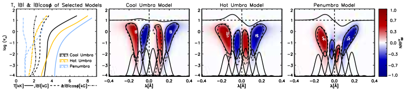
Figure 7.— From left to right, the $1^{st}$ panel shows the temperature (thick line), the magnetic field strength (dashed line), and the product $|B|cos\phi_{B}$ (dot-dashed line) through the atmosphere of the semi-empirical models used to calculate the normalized response functions of Stokes V to the magnetic field strength ($NRF^{V}_{|B|}$). The $2^{nd},3^{rd}$ and $4^{th}$ panels show the $NRF^{V}_{|B|}$ for Fe I 6302Å. The thick-lined contours show the regions where the $|NRF^{V}_{|B|}|$ are larger than 0.2 for Fe I 6302Å, and the dash-lined contours do for Fe I 6173Å. The location of the maximum and minimum of the $NRF^{V}_{|B|}$ for those lines are marked by a ”S” (SP) and a ”H” (HMI).

One possible scenario might explain the values of ${<}b{>}\$in the comparison between $\mathbf{B^{\mathbf{HMI}}_{\mathbf{Z}}}$  and $\mathbf{B^{\mathbf{SP}}_{\mathbf{Z}}}$ . In an ideal vertical flux tube in the photosphere, the magnetic field strength observed along the line of sight decreases as it expands in the higher layers. Thus, if the region where the spectral line Fe I 6302 Å is sensitive to the magnetic field is slightly lower than the region where the line Fe I 6173 Å is, then SP would observed a slightly stronger magnetic field than the one observed by HMI.

Fleck et al. (2011) calculated the height formation of Fe I 6173 Å cross-correlating Doppler velocities observed by HMI with 3D radiation-hydrodynamic simulations. Taking into account the spatial resolution of the HMI Dopplergrams, the authors found the formation height of Fe I 6173 Å is about $140-150\ km$. On the other hand, several studies found the height formation for Fe I 6302 Å in higher layers of the photosphere. Shchukina & Trujillo Bueno (2001) found the height where the LTE optical depth at the line center is $\tau_{line}=1$ for Fe I 6302 Å to be $400\ km$ and $350\ km$ for a granule and intergranule, respectively. Grec et al. (2010) found the line formation height located between 138 to $201\ km$ for above the continuum formation height, and the height where optical depth is 1 for this line to be $244\ km$. Faurobert et al. (2012), found a variation of the formation height from $200\ km$ in the disk center to $470\ km$ close to the limb. In all these cases, the formation height of Fe I 6302 Å is higher than for Fe I 6173 Å.

Expressions such as “a spectral line is formed at a particular height in the solar atmosphere”, or in the best case, “a spectral line is formed within a given region” are an over-simplification of complex 3D physics (Judge et al., 2015). It is more precise to say “a spectral line is sensitive to a physical parameter in the region ranging from A to B”, where A and B are values of height given in an appropriate scale, e.g., geometrical or optical depth, and/or within a certain kind of magnetic structure (flux tube versus intergranular lane, for example). Several authors have addressed such ideas (Del Toro Iniesta & Ruiz Cobo, 1996; Sánchez Almeida & Landi Degl’Innocenti, 1996) by making use of response functions (RFs, Mein 1971; Beckers & Milkey 1975; Ruiz Cobo & del Toro Iniesta 1994). The RF is defined as the variation of a Stokes parameter with respect the variation of a physical atmospheric parameter at a given optical depth and wavelength. Borrero et al. (2014) compared the results obtained from three Milne-Eddington ICs with 3D MHD numerical simulations. The authors concluded that using generalized RFs to determine the height at which Milne-Eddington ICs measure physical parameters is more meaningful than comparisons of inverted parameters at a fixed height.

We have computed the RF of Stokes V to the magnetic field strength for those spectral lines using the SIR IC (Ruiz Cobo & del Toro Iniesta, 1992). That code computes the RFs under the assumption of local thermodynamic equilibrium, what is appropriate for the spectral lines investigated in this paper.

Figure 7 shows the behavior of temperature and the magnetic field strength with respect to the logarithm of the continuum optical depth at 5000Å. The following panels show the normalized RF of Stokes V to $|B|$ ($NRF^{V}_{|B|}$) for Fe I 6302 Å calculated using these models. The RF has been normalized to the maximum value of the RF of Stokes I to $|B|$. The thick contours delimit where the $|NRF^{V}_{|B|}|$ for Fe I 6302 Å is greater than 0.2. The dash-lined contours do for the $NRF^{V}_{|B|}$ calculated for Fe I 6173Å. Figure 7 shows that the region (expressed in $log(\tau_{c})$) where those lines are sensitive to the magnetic field strength are basically the same. The one corresponding to HMI extends a bit farther to higher layers, but just in the tail of the distribution of the NRF. The letters ”H” and ”S” pointed out the location of the minimum and maximum of the $NRF^{V}_{|B|}$ for HMI and SP respectively. These locations either overlap one to each other (cool umbra) or are significantly close in $log(\tau)$ and/or in spectral axis. The region where those lines are sensitive to $|B|$ is basically the same. The Stokes V profile for Fe I 6302 Å synthesized from the atmospheres used in this study, and the instrumental profiles used by HMI and in the pseudo-SP maps displayed as reference at the corresponding wavelength. One can argue about the difference in the spectral sampling used by the instruments. However, the comparison between SP and S2H does not show a such a significant difference between the ${<}b{>}\$for the horizontal components and the vertical one in the umbra and penumbra, being all the values very close to 1. Therefore, we are not able to explain why $\mathbf{B^{\mathbf{HMI}}_{\mathbf{Z}}}$  observes $\sim 0.85$ times the apparent longitudinal component of the magnetic field observed by SP, $\mathbf{B^{\mathbf{SP}}_{\mathbf{Z}}}$ .

We may speculate about the effects introduced by the main contributors in the RF of the Stokes V to the magnetic field strength following the analysis made by Cabrera Solana et al. (2005). The authors calculated the expression $RF^{V}_{|B|}$ based in a phenomenological model for the weak spectral lines. In the strong field regime, the $\sigma$ components of the Stokes V profile are represented by (Eq. 7 in Cabrera Solana et al. 2005):

$$V(\lambda)=\pm A^{V}_{0}exp\left[\frac{-(\lambda-\lambda_{0}\pm\lambda_{B})^{2}}{2(A^{V}_{1})^{2}}\right]$$ (1)

where $A^{V}_{0}$ and $A^{V}_{1}$ are the amplitude and width of the Stokes V lobes, and the Zeeman splitting is $\lambda_{B}=Cg_{eff}B\lambda^{2}_{0}$ , with $C\equiv 4.67\times 10^{-13}\AA^{-1}G^{-1}$ and B the magnetic field strength (assumed to be constant with height). The authors found the $RF^{V}_{|B|}$ reaches the maximum sensitivity in the winds of the $\sigma$ components of the Stokes V. Thus, for the negative sign of $A^{V}_{1}$ (Eq. 17 in Cabrera Solana et al. 2005):

$$R^{V}_{|B|}(\lambda_{max})=e^{−1/2}C\frac{A^{V}_{0}}{A^{V}_{1}}g_{eff}\lambda^{2}_{0}$$ (2)

with $e$ being the Euler’s number. Therefore, for the expression for the maximum sensitivity we should know the ratio between the amplitude and the width, and the Landé factor, $g_{eff}$, of the spectral line located at $\lambda_{0}$. Any variation introduced in those factors might change the response of the Stokes V to a variation in the magnetic field strength. Thus, the parameters $A^{V}_{0}$ and $A^{V}_{1}$ determined from an observation taken with HMI, i.e., with a coarse spectral sampling of $\sim 69m\AA$ in 6 points, may introduce a larger uncertainty than from an observation taken with SP, i.e., with a finer spectral sampling in more points in the spectral line.

3.4. Comparison Between the Apparent Longitudinal Magnetic Flux ($B_{app}$), Total Magnetic Flux ($\Phi$), and unsigned magnetic flux ($\widehat{\Phi}$), observed by HMI and SP. .

Table 5Comparison between the apparent magnetic flux density ($B_{app}$), the total magnetic flux ($\Phi$), and the total unsigned magnetic flux ($\widehat{\Phi}$) for HMI and SP. $B_{app}$ is given in $Mx/cm^{2}$. $\Phi$ and $\widehat{\Phi}$ are given in $10^{21}Mx$.

$\mathbf{Solar\ Feature}$	$B_{app}^{HMI}$ vs $B_{app}^{SP}$	$\mathbf{<s_{e}>}$	$\mathbf{<r>}$	$\mathbf{<r^{2}>}$
Umbra	$B^{HMI}_{app}=(-0.26\pm 0.07)+(0.84\pm 0.04)\times B^{SP}_{app}$	$0.09\pm 0.03$	$0.97\pm 0.02$	$0.93\pm 0.04$
Penumbra	$B^{HMI}_{app}=(-0.02\pm 0.01)+(0.95\pm 0.02)\times B^{SP}_{app}$	$0.09\pm 0.01$	$0.98\pm 0.01$	$0.96\pm 0.01$
Strong B Plage	$B^{HMI}_{app}=(-0.02\pm 0.01)+(0.32\pm 0.06)\times B^{SP}_{app}$	$0.09\pm 0.01$	$0.82\pm 0.02$	$0.67\pm 0.03$
Weak B Plage	$B^{HMI}_{app}=(-0.00\pm 0.00)+(0.32\pm 0.08)\times B^{SP}_{app}$	$0.05\pm 0.00$	$0.72\pm 0.03$	$0.51\pm 0.04$
$\mathbf{Solar\ Feature}$	$\Phi^{HMI}$ vs $\Phi^{SP}$	$\mathbf{s_{e}}$	$\mathbf{r}$	$\mathbf{r^{2}}$
Umbra	$\Phi^{HMI}=(-0.07\pm 0.02)+(0.93\pm 0.01)\times\Phi^{SP}$	$0.01\pm 0.01$	$1.00\pm 0.01$	$1.00\pm 0.01$
Penumbra	$\Phi^{HMI}=(0.20\pm 0.07)+(1.14\pm 0.05)\times\Phi^{SP}$	$0.04\pm 0.01$	$0.99\pm 0.01$	$0.98\pm 0.01$
Strong B Plage	$\Phi^{HMI}=(-0.04\pm 0.00)+(0.27\pm 0.08)\times\Phi^{SP}$	$0.02\pm 0.01$	$0.69\pm 0.01$	$0.47\pm 0.01$
Weak B Plage	$\Phi^{HMI}=(-0.01\pm 0.00)+(0.32\pm 0.03)\times\Phi^{SP}$	$0.01\pm 0.01$	$0.96\pm 0.01$	$0.91\pm 0.01$
$\mathbf{Solar\ Feature}$	$\widehat{\Phi}^{HMI}$ vs $\widehat{\Phi}^{SP}$	$\mathbf{s_{e}}$	$\mathbf{r}$	$\mathbf{r^{2}}$
Umbra	$\widehat{\Phi}^{HMI}=(0.07\pm 0.02)+(0.93\pm 0.01)\times\widehat{\Phi}^{SP}$	$0.01\pm 0.01$	$1.00\pm 0.01$	$1.00\pm 0.01$
Penumbra	$\widehat{\Phi}^{HMI}=(-0.23\pm 0.08)+(1.13\pm 0.05)\times\widehat{\Phi}^{SP}$	$0.03\pm 0.01$	$0.99\pm 0.01$	$0.98\pm 0.01$
Strong B Plage	$\widehat{\Phi}^{HMI}=(0.32\pm 0.04)+(0.08\pm 0.05)\times\widehat{\Phi}^{SP}$	$0.02\pm 0.01$	$0.45\pm 0.01$	$0.20\pm 0.01$
Weak B Plage	$\widehat{\Phi}^{HMI}=(0.08\pm 0.01)+(0.15\pm 0.02)\times\widehat{\Phi}^{SP}$	$0.01\pm 0.01$	$0.89\pm 0.01$	$0.79\pm 0.01$

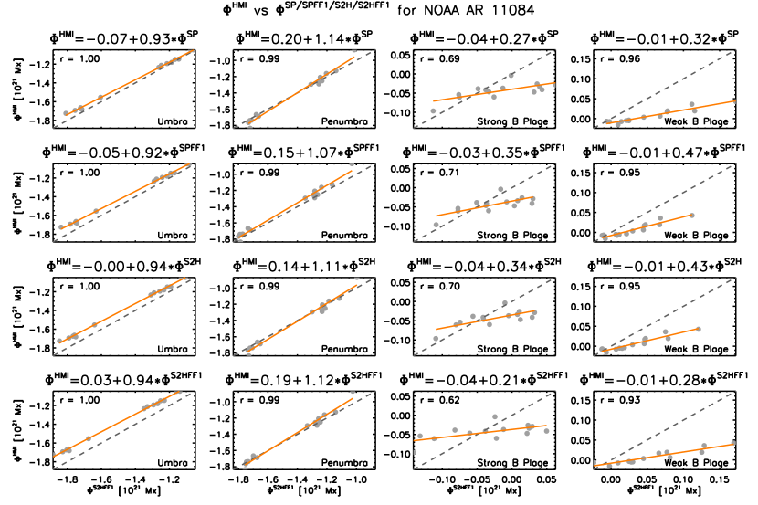
Figure 8.— Comparison between the total (signed) magnetic flux, $\Phi$, observed by HMI and SP, SPFF1, S2H, and S2HFF1. Values are given in $10^{21}Mx$.

We have studied the apparent longitudinal magnetic flux density, $\mathit{B_{app}}$, observed by HMI and SP, being $\mathit{B_{app}}=FF\times|\mathbf{B}|\times cos\phi_{B}$, and expressed in $Mx/cm^{2}$. We follow the notation and the conceptual interpretation given by Berger & Lites (2003), i.e.: “we denote calibrated magnetic flux density quantities as ‘B app’, the ‘apparent’ magnetic flux density measured by instrument ‘X’, in order to emphasize the inherent instrumental and observational limitations of the measurement.”

Table 5 shows the averaged statistical values of the linear regression between the apparent longitudinal magnetic flux measured by HMI and the one measured by SP in the RoIs. In addition, we present a similar comparison between HMI and the pseudo-SP maps in Table 13 in the Appendix, i.e. for the cases A to D in Table 2. It is obvious that in those cases where the FF is equal to one, the relationship between the $B_{app}^{HMI}$ and $B_{app}^{SPFF1}$ or $B_{app}^{S2HFF1}$, is the same as the one between the $\mathbf{B^{\mathbf{HMI}}_{\mathbf{Z}}}$  and $\mathbf{B^{\mathbf{SPFF1}}_{\mathbf{Z}}}$  or $\mathbf{B^{\mathbf{S2HFF1}}_{\mathbf{Z}}}$  respectively (see Table 10).

In the umbra and penumbra, the statistical values for the cases A to D are very similar, except for the averaged slope ${<}b{>}\$in the comparison between $B_{app}^{HMI}$ and $B_{app}^{SPFF1}$. The other statistical values show a very strong linear relationship between the apparent longitudinal magnetic flux density of the data compared, without a clear impact because of considering a different spectral line, spectral sampling, spatial sampling, filling factor or the other actors evaluated in the comparison. The apparent longitudinal magnetic flux observed by HMI in the umbra and penumbra is $84\%$ and $95\%$ respectively of the one observed by SP. The influence of FF in the calculation of $B_{app}$ is evident in the penumbra, where it is close to 1, but mostly different than 1, for the SP, while it is virtually equal to 1 everywhere in the umbra for the SP. Therefore, the relation $B_{app}^{HMI}$ and $B_{app}^{SP}$ in the umbra is similar to the relationship between $\mathbf{B^{\mathbf{HMI}}_{\mathbf{Z}}}$  and $\mathbf{B^{\mathbf{SP}}_{\mathbf{Z}}}$  in that RoI. The ${<}s_{e}{>}\$in both RoIs is $\sim 90Mx/cm^{2}$.

In the plage, the situation is slightly different. Again, the maps which consider a FF variable show lower averaged slope and lower averaged statistical values than the ones with a FF equal to 1. Although, that different behavior in the relationship of the $B_{app}$ observed by the maps with a different FF is little (e.g., less than $10\%$ in ${<}b{>}\$). Therefore, the linear relationship between the $B_{app}$ observed in the plage by HMI, both the strong and the weak plage, and the one observed by SP is moderate. In the strong and weak plage, HMI observes $32\%$ of the apparent longitudinal magnetic flux observed by SP, following a high-moderate linear relationship. The FF has a little impact in that relationship in the plage, while the other factors do not seem to play an important role in it. The ${<}s_{e}{>}\$in the strong plage is $\sim 90Mx/cm^{2}$, and $\sim 50Mx/cm^{2}$ in the weak plage.

Since the errors in the averaged slope and the statistical values in all the RoIs are small, we can conclude that the behavior in the relationship between $B_{app}^{HMI}$ and $B_{app}^{SP}$ is consistent through the maps analyzed in this study. That means, between $0.7<\mu<1$, the relationship between $B_{app}^{HMI}$ and $B_{app}^{SP}$ is strong in the umbra and penumbra, being in the plage moderate in the high range.

The sub-table in the middle of Table 5 shows the relationship between the total magnetic flux $\Phi$ observed by HMI and SP. Similarly, we have done that comparison between HMI and the pseudo-SP maps (see sub-table in the bottom of Table 13 in the Appendix). In these comparisons, one linear regression fit is calculated for each RoIs of the 14 analyzed maps. As in the rest of this paper, the RoIs are the areas of the umbra, penumbra, plage with a strong field, and plage with a weak field. As all the maps, after being corrected to match to each other, they share the same spatial scale. Therefore, the area used to calculate the total flux in the (compared) maps is the same. Of course, the value of the magnetic field inside these areas is what differs from one map to the other. Figure 8 shows the values for the total magnetic flux for the RoIs observed by HMI, SP and the pseudo-SP maps and the linear regression fit between them. The values of $\Phi$ in the panels of Fig. 8 and in Table 13 are expressed in $10^{21}Mx$. Note that in this case, we are doing the linear regression fit over 14 values corresponding to the 14 studied maps. Therefore, the intercept, slope and statistical values ($s_{e},r,r^{2}$) are not average values since they correspond to only one linear fit. The errors in the intercept and the slope are the standard errors defined for a linear regression fit. The errors of $s_{e},r,r^{2}$ are the rounding error in these values.

HMI observes $93\pm 1\%$ of the total magnetic flux observed by SP ($\Phi^{SP}$) in the umbra. However, for the penumbra, HMI overestimates in $14\pm 5\%$ the $\Phi^{SP}$. The statistical values show a very strong linear relationship between $\Phi^{HMI}$ and $\Phi^{SP}$ both in the umbra and penumbra. Similar behavior is observed in the comparison between $\Phi^{HMI}$ and the total magnetic flux of the pseudo-SP maps (see Table 13). In the strong and weak plage, HMI observes $\sim 30\%$ of the total magentic flux observed by SP. However, in the strong plage the correlation is moderate, while in the weak plage the correlation is very strong (${<}r{>}\$= $0.96\pm 0.01$). Similar behavior is observed in the comparison between $\Phi^{HMI}$ and the pseudo-SP maps.

In the bottom of Table 5, we show the comparison between the unsigned total magnetic flux measured by HMI, $\widehat{\Phi}^{HMI}$ and the one measured by SP, $\widehat{\Phi}^{SP}$, in the different RoIs. The values for the umbra and penumbra are very similar to the ones presented for the total magnetic flux. In these RoIs, as we have proven in Section 3.1, the magnetic field vector observed by HMI and SP are very similar (see top panels in Fig. 4). The most striking value in the comparison between $\widehat{\Phi}^{HMI}$ and $\widehat{\Phi}^{SP}$ are the ones corresponding to the strong plage. There, the slope, ${<}b{>}\$, is $0.08\pm 0.05$, and the variation of $\widehat{\Phi}^{HMI}$ explained by that relationship is around just the $20\%$. The values for the weak plage are slightly larger. The sub-table in the bottom of Table 13 in the Appendix shows similar comparisons between the unsigned total magnetic flux measured by HMI and the one measured by SPFF1, S2H and S2HFF1. Those comparisons may help us to understand what happens in the plage for the comparison between $\widehat{\Phi}^{HMI}$ and $\widehat{\Phi}^{SP}$. The statistical values for the comparison between $\widehat{\Phi}^{HMI}$ and $\widehat{\Phi}^{SPFF1}$ and $\widehat{\Phi}^{S2HFF1}$ in the strong plage are larger than those considering FF variable, but they are still considerably smaller than the corresponding ones in the weak plage. If we look in detail the vertical component of the map showed in Fig. 4, we can many pixels showing strong values (dark blue and dark red) in the SP and S2H maps that they are associated with smaller values in HMI (and in SPFF1 and S2HFF1). While the slopes in the relationships between $\mathbf{B^{\mathbf{HMI}}_{\mathbf{Z}}}$  and $\mathbf{B^{\mathbf{SP}}_{\mathbf{Z}}}$  for the strong and weak plage are similar (${<}b{>}\$$\sim 0.15$), the total sum of the unsigned flux in the locations showing strong values in SP shall be significantly larger than for the same locations at HMI, and a bit smaller if we consider FF fixed to 1. On the other hand, those locations showing weak values in HMI, i.e. the weak plage, have also associated weak values in SP. Therefore, the correlation between the total flux is better for the weak values, i.e. the weak plage, than for the strong values, i.e. the strong plage. Thus, the ${<}r{>}\$values are again, as for $\Phi$, larger for the weak plage than for the strong plage. In addition, the significant difference between the ${<}r{>}\$values in the strong and the weak plage may be due to the difference in the area defined as strong plage in the HMI maps and the one defined in the SP and S2H maps.

3.5. Comparison Between the Apparent Longitudinal Magnetic Flux ($B_{app}$), Total Magnetic Flux ($\Phi$), and unsigned magnetic flux ($\widehat{\Phi}$), observed by SP and pseudo-SP data.

In this section, we discuss the comparison of $B_{app}$, $\Phi$, and $\widehat{\Phi}$ obtained for SP, SPFF1, S2H and S2H data, i.e. corresponding to the comparisons E to H of Table 2. The comparison of those magnitudes for the case E (SP vs SPFF1) is particularly interesting, and they are shown in Table 6. Notice that the only difference between SP and SPFF1 is the way the FF was considered during the inversion od the Stokes profiles, being variable for the SP data, and fixed to 1 for SPFF1. All other actors are exactly the same.

The apparent longitudinal magnetic flux in the umbra is similar either considering FF fixed to one or variable. As we have mentioned, in the umbra the values of FF, when it is considered variable, are virtually equal to 1 in most of the pixels, and close, but different, to 1 in the penumbra. In this RoI, the $B_{app}^{SPFF1}$ shows an overestimation of $6\%$ with respect to $B_{app}^{SP}$. On the plage, things are different. Considering the FF fixed to 1 produce an underestimation in the apparent longitudinal magnetic flux $B_{app}^{SPFF1}$ of $\sim 18\%$ and $\sim 26\%$ in the strong and weak plage with respect to the case considering a FF variable, $B_{app}^{SP}$.

For the total magnetic flux and the total unsigned magnetic flux, we observe a similar behavior, i.e. a small overestimation ($\sim 5\%$) for the relationship of those magnitudes in the penumbra, and an important underestimation in the strong ($\sim 60\%$ for both magnitudes) and weak ($\sim 60\%$ for $\Phi$, and $\sim 45\%$ for $\widehat{\Phi}$) plage when considering a FF fixed to 1 instead of being variable. That means, the underestimation in these magnitudes in the plage appears (in this comparison) only because of the way the inversion is made, i.e. how the FF is considered. Therefore, we have to keep in mind this effect when we compare those magnitudes for HMI (FF fixed to 1) and SP (FF variable) data in Table 6.

Table 6Comparison between the apparent longitudinal magnetic flux density ($B_{app}$), the total magnetic flux ($\Phi$), and the total unsigned magnetic flux ($\widehat{\Phi}$) for SP and SP with FF=1. $B_{app}$ is given in $Mx/cm^{2}$. $\Phi$ and $\widehat{\Phi}$ are given in $10^{21}Mx$.

$\mathbf{Solar\ Feature}$	$B_{app}^{SPFF1}$ vs $B_{app}^{SP}$	$\mathbf{<s_{e}>}$	$\mathbf{<r>}$	$\mathbf{<r^{2}>}$
Umbra	$B^{SPFF1}_{app}=(-0.07\pm 0.05)+(0.98\pm 0.02)\times B^{SP}_{app}$	$0.03\pm 0.01$	$1.00\pm 0.00$	$0.99\pm 0.00$
Penumbra	$B^{SPFF1}_{app}=(0.01\pm 0.00)+(1.05\pm 0.01)\times B^{SP}_{app}$	$0.03\pm 0.01$	$1.00\pm 0.00$	$1.00\pm 0.00$
Strong B Plage	$B^{SPFF1}_{app}=(-0.01\pm 0.00)+(0.82\pm 0.04)\times B^{SP}_{app}$	$0.07\pm 0.01$	$0.98\pm 0.00$	$0.96\pm 0.00$
Weak B Plage	$B^{SPFF1}_{app}=(-0.00\pm 0.00)+(0.74\pm 0.07)\times B^{SP}_{app}$	$0.03\pm 0.00$	$0.95\pm 0.01$	$0.90\pm 0.01$
$\mathbf{Solar\ Feature}$	$\Phi^{SPFF1}$ vs $\Phi^{SP}$	$\mathbf{<s_{e}>}$	$\mathbf{<r>}$	$\mathbf{<r^{2}>}$
Umbra	$\Phi^{SPFF1}=(-0.02\pm 0.00)+(1.00\pm 0.00)\times\Phi^{SP}$	$0.00\pm 0.01$	$1.00\pm 0.01$	$1.00\pm 0.01$
Penumbra	$\Phi^{SPFF1}=(0.05\pm 0.01)+(1.06\pm 0.00)\times\Phi^{SP}$	$0.00\pm 0.01$	$1.00\pm 0.01$	$1.00\pm 0.01$
Strong B Plage	$\Phi^{SPFF1}=(-0.02\pm 0.00)+(0.66\pm 0.04)\times\Phi^{SP}$	$0.01\pm 0.01$	$0.98\pm 0.01$	$0.96\pm 0.01$
Weak B Plage	$\Phi^{SPFF1}=(-0.00\pm 0.00)+(0.61\pm 0.04)\times\Phi^{SP}$	$0.00\pm 0.01$	$0.98\pm 0.01$	$0.96\pm 0.01$
$\mathbf{Solar\ Feature}$	$\widehat{\Phi}^{SPFF1}$ vs $\widehat{\Phi}^{SP}$	$\mathbf{<s_{e}>}$	$\mathbf{<r>}$	$\mathbf{<r^{2}>}$
Umbra	$\widehat{\Phi}^{SPFF1}=(0.02\pm 0.00)+(1.00\pm 0.00)\times\widehat{\Phi}^{SP}$	$0.00\pm 0.01$	$1.00\pm 0.01$	$1.00\pm 0.01$
Penumbra	$\widehat{\Phi}^{SPFF1}=(0.01\pm 0.01)+(1.03\pm 0.00)\times\widehat{\Phi}^{SP}$	$0.00\pm 0.01$	$1.00\pm 0.01$	$1.00\pm 0.01$
Strong B Plage	$\widehat{\Phi}^{SPFF1}=(0.18\pm 0.02)+(0.60\pm 0.02)\times\widehat{\Phi}^{SP}$	$0.01\pm 0.01$	$0.99\pm 0.01$	$0.99\pm 0.01$
Weak B Plage	$\widehat{\Phi}^{SPFF1}=(0.10\pm 0.01)+(0.44\pm 0.04)\times\widehat{\Phi}^{SP}$	$0.01\pm 0.01$	$0.95\pm 0.01$	$0.89\pm 0.01$

To evaluate the effect of other actors, we have made the comparison of these magnitudes between SP and pseudo-SP data, as are described to the case E to H in Section 2.3. The statistical values of these comparison are showed in the Table 14 of the Appendix. We can compare the values corresponding to the case G (S2HFF1 vs SP) with the values of the case A (HMI vs SP, Table 5), since the S2HFF1 are the closest data to HMI. Thus, if we take the pair of values of ${<}b{>}\$($\%$) for the relationship of those magnitudes at the strong and weak plage in the case A as ${<}b{>}\$(strong/weak plage) [$B_{app}=32/32,\phi=27/32,\widehat{\phi}$ = 8/15 ], while for the case G is ${<}b{>}\$(strong/weak plage) [$B_{app}=79/72,\phi=54/64,\widehat{\phi}$ = 55/50]. The difference between these values may be explained in terms of the different actors not included either in the comparison A or G, that means: the spatial sampling, the spectral line and the S/N. In other words, the largest difference comes from considering the FF variable or fixed to 1, then the spectral sampling, finally the other actors. As we have showed in the Section 3.3.1, the lines observed by HMI and SP shows a similar response variation to the magnetic field, so we should expect a similar magnetic flux observed by those lines. We have to concluded that the spatial resolution and the S/N are the last actors (in importance) in the list of contributors to the difference in the comparison of $B_{app}$, $\phi$, and $\widehat{\phi}$.

4. Conclusions

We have compared the vector magnetic field observed by HMI with the one observed by SP. In addition, we have used pseudo-SP data to know about the role played for the actors what differ between the original HMI and SP data sets. These actors are summarized in Table 2. We have to admit that other actors may introduce an effect in an eventual comparison between HMI and SP data, e.g.: the temporal evolution of solar structures during the scan of SP. Thus, while we have done our best to analyze, explain and quantify the effects of the actors mentioned in the Table 2, we cannot guarantee that other actors may introduce an effect in our results. However, in a comparisons between HMI and SP data similar to the ones used in this study (temporal sampling, solar structures in the field of view, S/N, etc.), we expect similar results to the ones found in this study.

Our results are divided in two parts. On one side, the results concerning to the data available to the public as they are. On the other side, the results that provide a better understanding of the instrumental and treatment effects on the original data. Since, we have applied the same methodology – a linear regression fit – to the analyzed data set (14 quasi-simultaneous maps of NOAA AR 11084), our results must be understood in a statistical sense. Our study has been carried out comparing the Cartesian and the spherical components of the vector magnetic field obtained from one instrument to the other. Through the comparison of the spherical components, we earn a better understanding of the effect introduced by the disambiguation of the azimuth. All our results are referred to both system of coordinates, since they are complementary and consistent between them, but here we summarize them referring to the Cartesian coordinates.

Table 3 and 4 show the linear relationship between the components – Cartesian and spherical respectively– of the vector magnetic field $\mathbf{B^{\mathbf{HMI}}_{\mathbf{}}}$  and $\mathbf{B^{\mathbf{SP}}_{\mathbf{}}}$  in four different regions: umbra, penumbra, plage with a strong magnetic field, and plage with a weak magnetic field. The values of the straightforward comparison, the averaged statistical values and the errors found for those relationships. Similarly, Table 5 shows the relation between the apparent longitudinal magnetic flux, the signed and unsigned total magnetic flux measured by HMI and SP. Here, in the sake of simplicity, we present our findings as an approximation of those values. While Tables 3, 4 and 5 represent the main findings of this investigation –visually supported by Figs. 4, 5 and 6 –, we summarize here the physical meaning of our results.

Table 1 shows the ranges of the values in the RoIs compared in this study. We have to consider our results valid in those intervals, and different behavior may happen in regions with different ranges of values. For instance, larger cool umbrae with higher magnetic field strengths than the one used in this study may present molecular spectral bands that likely influence MERLIN or VFISV magnetic field inversions.

In the umbra and penumbra, the components of the vector magnetic field observed by HMI and SP are very similar. They are showing a strong linear correlation, having an averaged slope very close to 1 for the horizontal components and $\sim 0.83$ for the vertical component. After a detailed study, we can only speculate about the origin of that difference in the averaged slope. We feel inclined to believe that difference comes from the spectral sampling of HMI and the uncertainty introduced by sampling the Stokes V profile, therefore the region where the atmosphere is sensitive to the magnetic field. The averaged standard deviation about the least squares line for the components of the predicted $\mathbf{B^{\mathbf{HMI}}_{\mathbf{}}}$ , ${<}s_{e}{>}\$, is $\sim 100G$ both in the umbra and penumbra. In the umbra, the apparent longitudinal magnetic flux observed by HMI, $B_{app}^{HMI}$, is $84\%$ of the one observed by SP, $B_{app}^{SP}$. In the penumbra, $B_{app}^{HMI}$ observes $95\%$ of $B_{app}^{SP}$. In both RoIs, the relationship between these variables is very strong ($\sim 0.98$). The signed and unsigned total flux measured by HMI is underestimating the one measured by SP in the umbra in about $\sim 7\%$, and overestimating it in the penumbra about $\sim 14\%$.

For the plage hosting strong magnetic field, i.e., in those pixels in the plage where $200G<(\mid$ $\mathbf{B^{\mathbf{HMI}}_{\mathbf{XYZ}}}$ $\mid$ or $\mid$ $\mathbf{B^{\mathbf{SP}}_{\mathbf{XYZ}}}$ $\mid)<1000G$, we have found a moderate linear relationship between $\mathbf{B^{\mathbf{HMI}}_{\mathbf{XYZ}}}$  and $\mathbf{B^{\mathbf{SP}}_{\mathbf{XYZ}}}$ . The averaged standard deviation about the least squares line for the predicted $\mathbf{B^{\mathbf{HMI}}_{\mathbf{}}}$  is $\sim 160G$ for the horizontal components, and $70G$ for the vertical component. The linear relationships found are able to explain about $40\%$ of the variation of the predicted $\mathbf{B^{\mathbf{HMI}}_{\mathbf{XY}}}$  and $50\%$ for the $\mathbf{B^{\mathbf{HMI}}_{\mathbf{Z}}}$ . The errors in the averaged slope and the averaged statistical parameters of the horizontal components are significantly larger than the errors for the vertical component. That means, the distribution of those parameters for the 14 maps is more scattered for the horizontal components than for the vertical one. In the plage, HMI measures $32\%$ of the apparent longitudinal magnetic flux measured by SP, with an averaged standard deviation about the least squares line for the predicted ${B^{HMI}_{app}}$ is $90Mx/cm^{2}$. Both the apparent magnetic flux and the (signed) total magnetic flux measured by HMI and SP show a strong linear correlation, while the unsigned total magnetic flux shows a weak correlation with a very small slope $\sim 0.08$. In other words, in the strong plage HMI measures just $8\%$ of the unsigned total magnetic flux observed by SP in that RoI.

For the plage where the magnetic field is weak, i.e., in those pixels in the plage where $(\mid$ $\mathbf{B^{\mathbf{HMI}}_{\mathbf{XYZ}}}$ $\mid$ or $\mid$ $\mathbf{B^{\mathbf{SP}}_{\mathbf{XYZ}}}$ $\mid)<200G$, the relationship between $\mathbf{B^{\mathbf{HMI}}_{\mathbf{XY}}}$  and $\mathbf{B^{\mathbf{SP}}_{\mathbf{XY}}}$  is weak, while between $\mathbf{B^{\mathbf{HMI}}_{\mathbf{Z}}}$  and $\mathbf{B^{\mathbf{SP}}_{\mathbf{Z}}}$  is moderate. The averaged standard deviation about the least squares line for the predicted $\mathbf{B^{\mathbf{HMI}}_{\mathbf{}}}$  is $100G$ for the horizontal components, and $50G$ for the vertical component. Note the large values of ${<}s_{e}{>}\$for the horizontal components, meaning that there is a large scatter around the least squares line. The errors in the averaged slope and the averaged statistical parameters of the horizontal components are significantly larger than the errors of the vertical component. That is, the distribution of those parameters for the 14 maps is more scattered for the horizontal components than for the vertical one. In the weak plage, the linear relationship between $B_{app}^{HMI}$ and $B_{app}^{SP}$ is high-moderate, while the relationships between $\Phi^{HMI}$ and $\Phi^{SP}$, and between $\widehat{\Phi}^{HMI}$ and $\widehat{\Phi}^{SP}$ are very strong. The averaged standard deviation about the least squares line for ${B^{HMI}_{app}}$ is $50Mx/cm^{2}$.

From the comparison between HMI and the psesudo-SP maps, we conclude that the actor having a major impact in the statistical values analyzed is the filling factor, followed by the spectral sampling, and finally the spatial sampling. The effect introduced by the FF is important especially in the plage. Thus, if the magnetic field observed by HMI and the corresponding for SP where both calculated with an inversion considering FF equal to 1, the improvement in the explained variation of HMI by SP would be of $\sim 20\%$ in the strong plage for all the components of $\mathbf{B^{\mathbf{HMI}}_{\mathbf{}}}$ , and $9\%$ and $19\%$ for the horizontal and vertical components respectively in the weak plage. The improvements in the explained variation of corresponding predicted variables are larger between HMI and the maps of SP sampled as HMI does (both S2H and S2HFF1) than between HMI and SPFF1. However, the slope for the horizontal component are worse than for the comparison between HMI and SP with FF=1. The biggest improvements in all the statistical values comes from considering both FF equal to 1 and same spectral sampling between HMI and SP, i.e. when the SP data become closest to HMI data.

Considering the FF fixed to 1 or variable on the same data (SPFF1 $vs$ SP) has an important impact in the apparent longitudinal magnetic flux, the total flux and the total unsigned flux. The apparent longitudinal magnetic flux ($B_{app}$) is overestimated by $5\%$ in the penumbra, underestimated by $18\%$ in the strong plage, and underestimated by $26\%$ in the weak plage when the magnetic field has been obtained considering a FF fixed to 1 ($B_{app}^{SPFF1}$), compared with when the FF is variable ($B_{app}^{SP}$). The total magnetic flux and the unsigned total magnetic flux have a similar behavior in those regions.

The error introduced by different disambiguation methods is negligible in the umbra and penumbra. While for the plage, the scatter introduced by the different resolved azimuth is smaller than the scatter introduced by the other actors. Nevertheless, if we compare only those pixels sharing the same sign after the disambiguation, the positive impact in all the variables might be important. For the comparison between the original HMI and SP data, the improvement in the explained variation of the horizontal components of the predicted $\mathbf{B^{\mathbf{HMI}}_{\mathbf{}}}$  with respect considering all the pixels is $\sim 40\%$ and $\sim[20-35]\%$ in the strong and weak plage. If we simply inverted the SP data with a FF fixed to 1, as HMI does, the correlation coefficients for between the horizontal components in those pixels sharing the same sign in both maps become ${<}r{>}\$$\sim 0.92$ and $\sim 83$ for the strong and the weak plage. comparison between HMI and S2HFF1, the explained variation of the horizontal components of the predicted $\mathbf{B^{\mathbf{HMI}}_{\mathbf{}}}$  becomes $\sim 85\%$ and $67\%$ in the strong and the weak plage respectively.

Using different disambiguation methods, we have found that about $\sim 25\%$ and $\sim 35\%$ of the pixels in the plage observed and disambiguated by HMI have an opposite sign with respect to the ones observed and disambiguated by SP. Similar values are obtained even when the same data (SP) are disambiguated using different methods (AMBIG $vs$ AZAM). The analysis of the disambiguation of the azimuth has proved that the opposite sign in the horizontal components of those structures in the plage is due to use different disambiguation methods, and not to opposite values of the pre-disambiguation azimuth. We suggest to investigate the option to use the same disambiguation code to solve the azimuth observed by HMI and SP data. That would improve the results of a comparison between them, especially in the plage, but, more important, it would favor the quasi-simultaneous and complementary use of both data.

In summary, the correlation between the components of the magnetic field observed by HMI and the ones observed by SP are very high in the umbra and penumbra, while it is moderate and weak for the strong and weak magnetic field of the plage respectively. Similar behavior happens for the apparent magnetic field and the total flux. The uncertainty in predicting $\mathbf{B^{\mathbf{HMI}}_{\mathbf{}}}$ , $B_{app}^{HMI}$, $\Phi^{HMI}$ and $\widehat{\Phi}^{HMI}$ from the respective values observed by SP becomes larger as we move from the regions with strong magnetic field and a filling factor closer to 1, to the regions where the magnetic field is weaker and the filling factor either is closer to 0 or more difficult to determine, i.e. as the observation goes from the umbra to the penumbra, then from there to strong plage, and finally from there to the weak plage. The only exception to this behavior happens in the statistical values of the comparison between $\Phi^{HMI}$ vs $\Phi^{SP}$ and $\widehat{\Phi}^{HMI}$ vs $\widehat{\Phi}^{SP}$ in the strong plage, which are worse than the ones corresponding to the weak plage.

Considering inversions with a similar treatment for the filling factor and the disambiguation of the azimuth would improve significantly the comparison between the vector magnetic field observed by HMI and SP. However, to consider a FF variable for HMI data may be not reliable due to S/N constrain (more than for the fact of using 6 spectral points). A careful study would be necessary to implement or discard this option. For the apparent longitudinal magnetic flux and the total flux, the impact of the filling factor, the spectral sampling and their combination is very little, being again the filling factor the most important actor.

In this appendix we show information about the data, detailed statistical values for the straightforward comparison between HMI and SP, and the averaged statistical values for the comparison between HMI and the pseudo-SP data. Despite the tediousness that all this information may represent for the reader, we consider it valuable for supporting our study and results.

Appendix A Data Selection

Table 7 shows the observation date ($1^{st}\$column), the starting time and the middle time for the scan in the SP instrument ($2^{nd}\$and $3^{rd}\$columns), and the closest in time HMI filtergram to the latter one ($4^{th}$ column). The positions of the selected maps are given in heliocentric coordinates ($5^{th}$ column), and by $\mu=cos(\theta)$, being $\theta$ the heliocentric angle ($6^{th}$ column). The size of the SP maps is given in $\arcsec\times\arcsec$ ($7^{th}$ column).

Table 7Information about the observation of NOAA AR 11084 by HMI and SP. See Section A for details.

Observation Date	SP Scan Starting Time	SP Scan Middle Time	Selected HMI Time	(X,Y)	$\mu$	SP Scan Size
(YYYY-MM-DD)	(hh:mm:ss)	(hh:mm:ss)	(hh:mm:ss)	(”,”)		” $\times$ ”
2010-06-29	11:20:21	11:32:31	11:36:08	(-561.056, -361.810)	0.707	113$\times$123
2010-06-29	16:20:06	16:32:38	16:36:08	(-528.149, -363.336)	0.736	110$\times$123
2010-07-01	21:15:40	21:28:00	21:24:08	(-129.088, -385.262)	0.902	111$\times$123
2010-07-01	23:55:50	00:07:59	00:12:08	(-106.956, -385.596)	0.905	114$\times$123
2010-07-02	05:15:05	05:27:07	05:24:08	(-062.809, -386.210)	0.910	113$\times$123
2010-07-02	13:15:05	13:27:15	13:24:08	(003.894, -386.894)	0.912	114$\times$123
2010-07-02	21:50:05	22:02:14	22:00:08	(075.464, -387.295)	0.908	114$\times$123
2010-07-03	00:32:50	00:44:59	00:48:08	(097.943, -387.348)	0.906	114$\times$123
2010-07-04	14:50:53	15:02:59	15:00:08	(394.844, -394.879)	0.807	114$\times$123
2010-07-04	16:20:05	16:32:14	16:36:08	(405.776, -394.645)	0.801	114$\times$123
2010-07-04	18:14:35	18:26:41	18:24:08	(418.902, -394.319)	0.793	110$\times$123
2010-07-04	19:51:36	20:03:18	20:00:08	(431.805, -393.983)	0.787	109$\times$123
2010-07-04	21:26:32	21:38:41	21:36:08	(442.777, -393.740)	0.779	114$\times$123
2010-07-04	22:55:05	23:07:14	23:12:08	(453.321, -393.465)	0.772	114$\times$123
2010-07-05	03:50:05	04:02:31	04:00:08	(487.696, -392.457)	0.748	110$\times$123

Appendix B Individual Linear Regression Fits and Statistical Values for the Comparison HMI vs SP

Tables 8 and 9 show several statistical values about the linear regression fit for the regions of interest analyzed in the individual maps presented in Table 7. The statistical values ${<}b{>}\$, ${<}s_{e}{>}\$, ${<}r{>}\$and ${<}r^{2}{>}\$showed in the Table 3 are the mean (averaged) values calculated from the columns $2^{nd}$, $4^{th}$, $5^{th}$ and $6^{th}$ respectively. The errors presented in Table 3 are the standard error of the mean values of the the quantities showed in Tables 8 and 9.

Table 8Linear regression fit between the horizontal components of the vector magentic field observed by HMI and SP. Colums are as follows: 1) location of the enter of map given as $\mu=cos(\theta)$, being $\theta$ the heliocentric angle; 2) intercept ($a$) and slope ($b$) of the linear regression fit; 3) confidence interval at a $95\%$ confidence level for $a$ and $b$; 4) estimated standard error about the least squares line, $s_{e}$; 5) correlation coefficient, $r$; 6) coefficient of determination, $r^{2}$, and 7) Spearman’s rank correlation coefficient $r_{s}$.

$B_{X}$
	Umbra							Penumbra
$\mu$		(a,b)	(ci a,ci b)	$s_{e}$	r	$r^{2}$	$r_{S}$		(a,b)	(ci a,ci b)	$s_{e}$	r	$r^{2}$	$r_{S}$
0.708		$(-0.18,+1.02)$	$(\pm 0.03,\pm 0.02)$	$+0.13$	$+0.98$	$+0.97$	$+0.98$		$(+0.03,+0.93)$	$(\pm 0.00,\pm 0.01)$	$+0.11$	$+0.98$	$+0.97$	$+0.99$
0.903		$(+0.03,+0.96)$	$(\pm 0.01,\pm 0.01)$	$+0.09$	$+0.99$	$+0.99$	$+0.99$		$(+0.02,+0.96)$	$(\pm 0.00,\pm 0.00)$	$+0.10$	$+0.99$	$+0.98$	$+0.99$
0.906		$(-0.03,+0.99)$	$(\pm 0.01,\pm 0.01)$	$+0.12$	$+0.99$	$+0.98$	$+0.98$		$(+0.01,+0.95)$	$(\pm 0.00,\pm 0.00)$	$+0.09$	$+0.99$	$+0.98$	$+0.99$
0.910		$(-0.04,+0.99)$	$(\pm 0.01,\pm 0.01)$	$+0.08$	$+1.00$	$+0.99$	$+1.00$		$(+0.00,+0.96)$	$(\pm 0.00,\pm 0.00)$	$+0.10$	$+0.99$	$+0.98$	$+0.99$
0.912		$(-0.03,+0.97)$	$(\pm 0.01,\pm 0.01)$	$+0.08$	$+1.00$	$+0.99$	$+1.00$		$(+0.01,+0.95)$	$(\pm 0.00,\pm 0.00)$	$+0.09$	$+0.99$	$+0.98$	$+0.99$
0.909		$(-0.00,+0.96)$	$(\pm 0.01,\pm 0.01)$	$+0.09$	$+0.99$	$+0.99$	$+1.00$		$(-0.00,+0.96)$	$(\pm 0.00,\pm 0.00)$	$+0.08$	$+0.99$	$+0.99$	$+0.99$
0.907		$(+0.01,+0.98)$	$(\pm 0.01,\pm 0.01)$	$+0.08$	$+1.00$	$+0.99$	$+1.00$		$(-0.00,+0.97)$	$(\pm 0.00,\pm 0.00)$	$+0.08$	$+0.99$	$+0.99$	$+0.99$
0.807		$(+0.07,+0.98)$	$(\pm 0.01,\pm 0.01)$	$+0.07$	$+1.00$	$+0.99$	$+1.00$		$(-0.01,+0.97)$	$(\pm 0.00,\pm 0.01)$	$+0.10$	$+0.99$	$+0.98$	$+0.98$
0.801		$(+0.11,+0.99)$	$(\pm 0.01,\pm 0.01)$	$+0.08$	$+0.99$	$+0.99$	$+0.99$		$(-0.00,+0.98)$	$(\pm 0.00,\pm 0.01)$	$+0.11$	$+0.99$	$+0.98$	$+0.98$
0.793		$(+0.19,+1.01)$	$(\pm 0.01,\pm 0.01)$	$+0.09$	$+0.99$	$+0.99$	$+0.99$		$(+0.01,+0.99)$	$(\pm 0.01,\pm 0.01)$	$+0.12$	$+0.99$	$+0.97$	$+0.98$
0.788		$(+0.14,+0.98)$	$(\pm 0.01,\pm 0.01)$	$+0.08$	$+0.99$	$+0.99$	$+0.99$		$(+0.00,+0.99)$	$(\pm 0.01,\pm 0.01)$	$+0.12$	$+0.99$	$+0.97$	$+0.98$
0.780		$(+0.14,+1.00)$	$(\pm 0.01,\pm 0.01)$	$+0.07$	$+0.99$	$+0.99$	$+1.00$		$(-0.01,+0.99)$	$(\pm 0.01,\pm 0.01)$	$+0.12$	$+0.99$	$+0.97$	$+0.98$
0.773		$(+0.13,+1.00)$	$(\pm 0.01,\pm 0.01)$	$+0.08$	$+0.99$	$+0.99$	$+0.99$		$(-0.00,+0.98)$	$(\pm 0.00,\pm 0.01)$	$+0.11$	$+0.99$	$+0.97$	$+0.98$
0.749		$(+0.13,+1.01)$	$(\pm 0.01,\pm 0.01)$	$+0.08$	$+0.99$	$+0.99$	$+0.99$		$(+0.01,+0.97)$	$(\pm 0.00,\pm 0.01)$	$+0.10$	$+0.99$	$+0.98$	$+0.98$
	Strong Plage							Weak Plage
$\mu$		(a,b)	(ci a,ci b)	$s_{e}$	r	$r^{2}$	$r_{S}$		(a,b)	(ci a,ci b)	$s_{e}$	r	$r^{2}$	$r_{S}$
0.708		$(-0.01,+0.16)$	$(\pm 0.01,\pm 0.02)$	$+0.20$	$+0.34$	$+0.11$	$+0.30$		$(-0.02,+0.11)$	$(\pm 0.00,\pm 0.01)$	$+0.11$	$+0.26$	$+0.07$	$+0.33$
0.903		$(-0.03,+0.52)$	$(\pm 0.01,\pm 0.02)$	$+0.16$	$+0.73$	$+0.53$	$+0.71$		$(-0.03,+0.18)$	$(\pm 0.00,\pm 0.01)$	$+0.10$	$+0.32$	$+0.10$	$+0.32$
0.906		$(-0.04,+0.55)$	$(\pm 0.01,\pm 0.02)$	$+0.14$	$+0.79$	$+0.62$	$+0.76$		$(-0.04,+0.25)$	$(\pm 0.00,\pm 0.01)$	$+0.09$	$+0.43$	$+0.18$	$+0.41$
0.910		$(-0.02,+0.52)$	$(\pm 0.01,\pm 0.02)$	$+0.14$	$+0.77$	$+0.59$	$+0.75$		$(-0.03,+0.24)$	$(\pm 0.00,\pm 0.01)$	$+0.09$	$+0.42$	$+0.18$	$+0.41$
0.912		$(-0.02,+0.51)$	$(\pm 0.01,\pm 0.02)$	$+0.14$	$+0.76$	$+0.58$	$+0.74$		$(-0.03,+0.24)$	$(\pm 0.00,\pm 0.01)$	$+0.09$	$+0.44$	$+0.19$	$+0.42$
0.909		$(-0.01,+0.50)$	$(\pm 0.01,\pm 0.02)$	$+0.15$	$+0.74$	$+0.55$	$+0.72$		$(-0.01,+0.22)$	$(\pm 0.00,\pm 0.01)$	$+0.10$	$+0.40$	$+0.16$	$+0.41$
0.907		$(-0.02,+0.49)$	$(\pm 0.01,\pm 0.02)$	$+0.14$	$+0.75$	$+0.56$	$+0.70$		$(-0.02,+0.28)$	$(\pm 0.00,\pm 0.01)$	$+0.09$	$+0.48$	$+0.23$	$+0.49$
0.807		$(-0.04,+0.34)$	$(\pm 0.01,\pm 0.02)$	$+0.17$	$+0.62$	$+0.38$	$+0.59$		$(-0.02,+0.19)$	$(\pm 0.00,\pm 0.01)$	$+0.10$	$+0.41$	$+0.17$	$+0.46$
0.801		$(-0.04,+0.33)$	$(\pm 0.01,\pm 0.02)$	$+0.17$	$+0.60$	$+0.36$	$+0.58$		$(-0.03,+0.20)$	$(\pm 0.00,\pm 0.01)$	$+0.10$	$+0.42$	$+0.18$	$+0.48$
0.793		$(-0.04,+0.34)$	$(\pm 0.01,\pm 0.02)$	$+0.17$	$+0.63$	$+0.39$	$+0.61$		$(-0.02,+0.20)$	$(\pm 0.00,\pm 0.01)$	$+0.10$	$+0.44$	$+0.20$	$+0.50$
0.788		$(-0.03,+0.31)$	$(\pm 0.01,\pm 0.02)$	$+0.17$	$+0.57$	$+0.33$	$+0.56$		$(-0.02,+0.18)$	$(\pm 0.00,\pm 0.01)$	$+0.11$	$+0.40$	$+0.16$	$+0.46$
0.780		$(-0.03,+0.36)$	$(\pm 0.01,\pm 0.02)$	$+0.18$	$+0.61$	$+0.38$	$+0.58$		$(-0.02,+0.19)$	$(\pm 0.00,\pm 0.01)$	$+0.11$	$+0.41$	$+0.17$	$+0.46$
0.773		$(-0.04,+0.33)$	$(\pm 0.01,\pm 0.02)$	$+0.17$	$+0.61$	$+0.37$	$+0.58$		$(-0.02,+0.20)$	$(\pm 0.00,\pm 0.01)$	$+0.10$	$+0.41$	$+0.17$	$+0.48$
0.749		$(-0.04,+0.33)$	$(\pm 0.01,\pm 0.02)$	$+0.17$	$+0.62$	$+0.39$	$+0.58$		$(-0.02,+0.18)$	$(\pm 0.00,\pm 0.01)$	$+0.10$	$+0.39$	$+0.15$	$+0.44$
$B_{Y}$
	Umbra							Penumbra
$\mu$		(a,b)	(ci a,ci b)	$s_{e}$	r	$r^{2}$	$r_{S}$		(a,b)	(ci a,ci b)	$s_{e}$	r	$r^{2}$	$r_{S}$
0.708		$(-0.10,+1.02)$	$(\pm 0.01,\pm 0.01)$	$+0.10$	$+0.99$	$+0.98$	$+0.99$		$(-0.00,+0.95)$	$(\pm 0.00,\pm 0.01)$	$+0.09$	$+0.99$	$+0.98$	$+0.99$
0.903		$(-0.05,+1.01)$	$(\pm 0.01,\pm 0.01)$	$+0.08$	$+0.99$	$+0.99$	$+0.99$		$(+0.00,+1.00)$	$(\pm 0.00,\pm 0.01)$	$+0.10$	$+0.99$	$+0.98$	$+0.99$
0.906		$(-0.02,+0.98)$	$(\pm 0.02,\pm 0.02)$	$+0.14$	$+0.98$	$+0.96$	$+0.98$		$(+0.01,+0.97)$	$(\pm 0.00,\pm 0.00)$	$+0.09$	$+0.99$	$+0.98$	$+0.99$
0.910		$(-0.01,+0.99)$	$(\pm 0.01,\pm 0.01)$	$+0.08$	$+0.99$	$+0.99$	$+0.99$		$(-0.00,+0.95)$	$(\pm 0.00,\pm 0.01)$	$+0.13$	$+0.98$	$+0.96$	$+0.98$
0.912		$(-0.02,+0.99)$	$(\pm 0.01,\pm 0.01)$	$+0.09$	$+0.99$	$+0.99$	$+0.99$		$(+0.00,+0.95)$	$(\pm 0.00,\pm 0.01)$	$+0.10$	$+0.99$	$+0.98$	$+0.99$
0.909		$(-0.03,+0.98)$	$(\pm 0.01,\pm 0.01)$	$+0.10$	$+0.99$	$+0.98$	$+0.99$		$(+0.00,+0.98)$	$(\pm 0.00,\pm 0.00)$	$+0.09$	$+0.99$	$+0.98$	$+0.99$
0.907		$(-0.01,+0.99)$	$(\pm 0.01,\pm 0.01)$	$+0.08$	$+0.99$	$+0.99$	$+0.99$		$(+0.01,+0.96)$	$(\pm 0.00,\pm 0.00)$	$+0.09$	$+0.99$	$+0.98$	$+0.99$
0.807		$(+0.02,+0.96)$	$(\pm 0.01,\pm 0.01)$	$+0.07$	$+0.99$	$+0.99$	$+0.99$		$(+0.01,+0.95)$	$(\pm 0.00,\pm 0.01)$	$+0.11$	$+0.99$	$+0.97$	$+0.99$
0.801		$(+0.05,+0.95)$	$(\pm 0.01,\pm 0.01)$	$+0.07$	$+0.99$	$+0.98$	$+0.99$		$(+0.02,+0.94)$	$(\pm 0.00,\pm 0.01)$	$+0.10$	$+0.99$	$+0.98$	$+0.99$
0.793		$(+0.02,+0.95)$	$(\pm 0.01,\pm 0.01)$	$+0.09$	$+0.99$	$+0.98$	$+0.99$		$(+0.02,+0.93)$	$(\pm 0.01,\pm 0.01)$	$+0.13$	$+0.98$	$+0.96$	$+0.98$
0.788		$(+0.00,+0.96)$	$(\pm 0.01,\pm 0.01)$	$+0.08$	$+0.99$	$+0.98$	$+0.99$		$(+0.03,+0.94)$	$(\pm 0.01,\pm 0.01)$	$+0.13$	$+0.98$	$+0.96$	$+0.98$
0.780		$(+0.02,+0.96)$	$(\pm 0.01,\pm 0.01)$	$+0.07$	$+0.99$	$+0.99$	$+0.99$		$(+0.02,+0.94)$	$(\pm 0.01,\pm 0.01)$	$+0.13$	$+0.98$	$+0.96$	$+0.98$
0.773		$(+0.04,+0.96)$	$(\pm 0.01,\pm 0.01)$	$+0.07$	$+0.99$	$+0.99$	$+0.99$		$(+0.02,+0.95)$	$(\pm 0.00,\pm 0.01)$	$+0.11$	$+0.99$	$+0.97$	$+0.98$
0.749		$(+0.02,+0.96)$	$(\pm 0.01,\pm 0.01)$	$+0.07$	$+0.99$	$+0.99$	$+0.99$		$(+0.00,+0.95)$	$(\pm 0.00,\pm 0.01)$	$+0.11$	$+0.99$	$+0.97$	$+0.99$
	Strong Plage							Weak Plage
$\mu$		(a,b)	(ci a,ci b)	$s_{e}$	r	$r^{2}$	$r_{S}$		(a,b)	(ci a,ci b)	$s_{e}$	r	$r^{2}$	$r_{S}$
0.708		$(+0.01,+0.26)$	$(\pm 0.01,\pm 0.02)$	$+0.18$	$+0.46$	$+0.21$	$+0.42$		$(+0.01,+0.14)$	$(\pm 0.00,\pm 0.01)$	$+0.10$	$+0.28$	$+0.08$	$+0.32$
0.903		$(-0.00,+0.23)$	$(\pm 0.01,\pm 0.02)$	$+0.17$	$+0.43$	$+0.19$	$+0.39$		$(-0.00,+0.11)$	$(\pm 0.00,\pm 0.01)$	$+0.10$	$+0.27$	$+0.07$	$+0.30$
0.906		$(-0.01,+0.24)$	$(\pm 0.01,\pm 0.02)$	$+0.16$	$+0.48$	$+0.23$	$+0.40$		$(-0.00,+0.11)$	$(\pm 0.00,\pm 0.01)$	$+0.09$	$+0.28$	$+0.08$	$+0.31$
0.910		$(+0.00,+0.27)$	$(\pm 0.01,\pm 0.02)$	$+0.16$	$+0.53$	$+0.28$	$+0.48$		$(-0.00,+0.14)$	$(\pm 0.00,\pm 0.01)$	$+0.10$	$+0.34$	$+0.11$	$+0.37$
0.912		$(+0.01,+0.26)$	$(\pm 0.01,\pm 0.02)$	$+0.16$	$+0.50$	$+0.25$	$+0.47$		$(-0.00,+0.14)$	$(\pm 0.00,\pm 0.01)$	$+0.09$	$+0.34$	$+0.12$	$+0.37$
0.909		$(+0.01,+0.25)$	$(\pm 0.01,\pm 0.02)$	$+0.16$	$+0.49$	$+0.24$	$+0.46$		$(+0.00,+0.15)$	$(\pm 0.00,\pm 0.01)$	$+0.09$	$+0.37$	$+0.14$	$+0.40$
0.907		$(+0.01,+0.29)$	$(\pm 0.01,\pm 0.02)$	$+0.17$	$+0.54$	$+0.30$	$+0.52$		$(+0.00,+0.17)$	$(\pm 0.00,\pm 0.01)$	$+0.10$	$+0.39$	$+0.15$	$+0.42$
0.807		$(+0.03,+0.38)$	$(\pm 0.01,\pm 0.02)$	$+0.15$	$+0.67$	$+0.45$	$+0.64$		$(+0.02,+0.19)$	$(\pm 0.00,\pm 0.01)$	$+0.09$	$+0.41$	$+0.17$	$+0.44$
0.801		$(+0.03,+0.39)$	$(\pm 0.01,\pm 0.02)$	$+0.16$	$+0.67$	$+0.45$	$+0.63$		$(+0.03,+0.20)$	$(\pm 0.00,\pm 0.01)$	$+0.09$	$+0.41$	$+0.17$	$+0.45$
0.793		$(+0.02,+0.41)$	$(\pm 0.01,\pm 0.02)$	$+0.15$	$+0.70$	$+0.49$	$+0.68$		$(+0.03,+0.17)$	$(\pm 0.00,\pm 0.01)$	$+0.10$	$+0.38$	$+0.15$	$+0.43$
0.788		$(+0.04,+0.37)$	$(\pm 0.01,\pm 0.02)$	$+0.16$	$+0.63$	$+0.40$	$+0.61$		$(+0.02,+0.19)$	$(\pm 0.00,\pm 0.01)$	$+0.10$	$+0.41$	$+0.16$	$+0.45$
0.780		$(+0.03,+0.41)$	$(\pm 0.01,\pm 0.02)$	$+0.16$	$+0.69$	$+0.47$	$+0.65$		$(+0.03,+0.20)$	$(\pm 0.00,\pm 0.01)$	$+0.09$	$+0.42$	$+0.17$	$+0.46$
0.773		$(+0.02,+0.42)$	$(\pm 0.01,\pm 0.02)$	$+0.16$	$+0.70$	$+0.49$	$+0.66$		$(+0.02,+0.21)$	$(\pm 0.00,\pm 0.01)$	$+0.10$	$+0.40$	$+0.16$	$+0.44$
0.749		$(+0.02,+0.43)$	$(\pm 0.01,\pm 0.02)$	$+0.16$	$+0.70$	$+0.48$	$+0.67$		$(+0.01,+0.22)$	$(\pm 0.00,\pm 0.02)$	$+0.10$	$+0.41$	$+0.17$	$+0.43$

Table 9Linear regression fit between the vertical component of the vector magentic field observed by HMI and SP. The meaning of the columns is the same as in Table 8.

$B_{Z}$
	Umbra							Penumbra
$\mu$		(a,b)	(ci a,ci b)	$\sigma$	r	$r^{2}$	$r_{S}$		(a,b)	(ci a,ci b)	$\sigma$	r	$r^{2}$	$r_{S}$
0.708		$(-0.30,+0.76)$	$(\pm 0.03,\pm 0.02)$	$+0.12$	$+0.97$	$+0.94$	$+0.97$		$(+0.00,+0.75)$	$(\pm 0.01,\pm 0.01)$	$+0.12$	$+0.96$	$+0.92$	$+0.96$
0.903		$(-0.17,+0.86)$	$(\pm 0.03,\pm 0.01)$	$+0.07$	$+0.98$	$+0.97$	$+0.98$		$(-0.03,+0.90)$	$(\pm 0.01,\pm 0.01)$	$+0.13$	$+0.96$	$+0.92$	$+0.95$
0.906		$(-0.18,+0.85)$	$(\pm 0.07,\pm 0.03)$	$+0.17$	$+0.91$	$+0.84$	$+0.96$		$(-0.02,+0.89)$	$(\pm 0.01,\pm 0.01)$	$+0.11$	$+0.97$	$+0.95$	$+0.96$
0.910		$(-0.08,+0.90)$	$(\pm 0.02,\pm 0.01)$	$+0.06$	$+0.99$	$+0.98$	$+0.99$		$(-0.01,+0.89)$	$(\pm 0.01,\pm 0.01)$	$+0.11$	$+0.97$	$+0.94$	$+0.96$
0.912		$(-0.17,+0.84)$	$(\pm 0.02,\pm 0.01)$	$+0.06$	$+0.99$	$+0.98$	$+0.99$		$(-0.01,+0.87)$	$(\pm 0.01,\pm 0.01)$	$+0.13$	$+0.96$	$+0.92$	$+0.95$
0.909		$(-0.18,+0.87)$	$(\pm 0.06,\pm 0.03)$	$+0.13$	$+0.94$	$+0.88$	$+0.97$		$(-0.02,+0.88)$	$(\pm 0.01,\pm 0.01)$	$+0.11$	$+0.97$	$+0.94$	$+0.97$
0.907		$(-0.05,+0.92)$	$(\pm 0.03,\pm 0.01)$	$+0.06$	$+0.99$	$+0.98$	$+0.99$		$(-0.02,+0.89)$	$(\pm 0.01,\pm 0.01)$	$+0.10$	$+0.98$	$+0.95$	$+0.97$
0.807		$(-0.22,+0.82)$	$(\pm 0.03,\pm 0.02)$	$+0.09$	$+0.97$	$+0.94$	$+0.96$		$(-0.01,+0.85)$	$(\pm 0.01,\pm 0.01)$	$+0.11$	$+0.98$	$+0.95$	$+0.98$
0.801		$(-0.26,+0.79)$	$(\pm 0.03,\pm 0.02)$	$+0.09$	$+0.96$	$+0.93$	$+0.95$		$(-0.01,+0.84)$	$(\pm 0.01,\pm 0.01)$	$+0.10$	$+0.98$	$+0.96$	$+0.98$
0.793		$(-0.35,+0.75)$	$(\pm 0.04,\pm 0.02)$	$+0.11$	$+0.95$	$+0.90$	$+0.92$		$(-0.02,+0.81)$	$(\pm 0.01,\pm 0.01)$	$+0.13$	$+0.97$	$+0.93$	$+0.97$
0.788		$(-0.39,+0.73)$	$(\pm 0.05,\pm 0.03)$	$+0.12$	$+0.93$	$+0.87$	$+0.89$		$(-0.03,+0.81)$	$(\pm 0.01,\pm 0.01)$	$+0.11$	$+0.97$	$+0.95$	$+0.98$
0.780		$(-0.32,+0.77)$	$(\pm 0.04,\pm 0.02)$	$+0.10$	$+0.96$	$+0.92$	$+0.93$		$(-0.03,+0.81)$	$(\pm 0.01,\pm 0.01)$	$+0.11$	$+0.97$	$+0.95$	$+0.98$
0.773		$(-0.29,+0.80)$	$(\pm 0.04,\pm 0.02)$	$+0.11$	$+0.96$	$+0.92$	$+0.93$		$(-0.03,+0.82)$	$(\pm 0.01,\pm 0.01)$	$+0.10$	$+0.98$	$+0.95$	$+0.98$
0.749		$(-0.25,+0.80)$	$(\pm 0.03,\pm 0.02)$	$+0.09$	$+0.97$	$+0.95$	$+0.95$		$(-0.02,+0.79)$	$(\pm 0.01,\pm 0.01)$	$+0.11$	$+0.98$	$+0.95$	$+0.98$
	Strong Plage							Weak Plage
$\mu$		(a,b)	(ci a,ci b)	$\sigma$	r	$r^{2}$	$r_{S}$		(a,b)	(ci a,ci b)	$\sigma$	r	$r^{2}$	$r_{S}$
0.708		$(-0.00,+0.15)$	$(\pm 0.00,\pm 0.01)$	$+0.07$	$+0.73$	$+0.54$	$+0.78$		$(+0.00,+0.13)$	$(\pm 0.00,\pm 0.00)$	$+0.05$	$+0.67$	$+0.44$	$+0.79$
0.903		$(-0.01,+0.13)$	$(\pm 0.00,\pm 0.00)$	$+0.07$	$+0.72$	$+0.52$	$+0.78$		$(-0.01,+0.09)$	$(\pm 0.00,\pm 0.00)$	$+0.05$	$+0.65$	$+0.42$	$+0.77$
0.906		$(-0.01,+0.12)$	$(\pm 0.00,\pm 0.00)$	$+0.06$	$+0.72$	$+0.52$	$+0.79$		$(-0.01,+0.09)$	$(\pm 0.00,\pm 0.00)$	$+0.05$	$+0.65$	$+0.43$	$+0.78$
0.910		$(-0.01,+0.12)$	$(\pm 0.00,\pm 0.00)$	$+0.06$	$+0.70$	$+0.49$	$+0.78$		$(-0.01,+0.08)$	$(\pm 0.00,\pm 0.00)$	$+0.05$	$+0.63$	$+0.40$	$+0.77$
0.912		$(-0.01,+0.14)$	$(\pm 0.00,\pm 0.00)$	$+0.07$	$+0.74$	$+0.55$	$+0.80$		$(-0.01,+0.09)$	$(\pm 0.00,\pm 0.00)$	$+0.05$	$+0.65$	$+0.42$	$+0.77$
0.909		$(-0.01,+0.15)$	$(\pm 0.00,\pm 0.00)$	$+0.07$	$+0.77$	$+0.60$	$+0.81$		$(-0.01,+0.09)$	$(\pm 0.00,\pm 0.00)$	$+0.05$	$+0.66$	$+0.44$	$+0.77$
0.907		$(-0.00,+0.16)$	$(\pm 0.00,\pm 0.01)$	$+0.08$	$+0.76$	$+0.57$	$+0.80$		$(-0.01,+0.09)$	$(\pm 0.00,\pm 0.00)$	$+0.05$	$+0.67$	$+0.45$	$+0.78$
0.807		$(-0.01,+0.15)$	$(\pm 0.00,\pm 0.01)$	$+0.07$	$+0.72$	$+0.52$	$+0.78$		$(-0.00,+0.11)$	$(\pm 0.00,\pm 0.00)$	$+0.05$	$+0.60$	$+0.36$	$+0.77$
0.801		$(-0.02,+0.15)$	$(\pm 0.00,\pm 0.01)$	$+0.08$	$+0.71$	$+0.50$	$+0.78$		$(-0.01,+0.11)$	$(\pm 0.00,\pm 0.00)$	$+0.05$	$+0.60$	$+0.37$	$+0.77$
0.793		$(-0.02,+0.14)$	$(\pm 0.00,\pm 0.01)$	$+0.08$	$+0.69$	$+0.48$	$+0.75$		$(-0.01,+0.10)$	$(\pm 0.00,\pm 0.00)$	$+0.06$	$+0.58$	$+0.33$	$+0.74$
0.788		$(-0.01,+0.16)$	$(\pm 0.00,\pm 0.01)$	$+0.08$	$+0.72$	$+0.52$	$+0.78$		$(-0.00,+0.11)$	$(\pm 0.00,\pm 0.00)$	$+0.06$	$+0.61$	$+0.38$	$+0.76$
0.780		$(-0.01,+0.15)$	$(\pm 0.00,\pm 0.01)$	$+0.08$	$+0.69$	$+0.47$	$+0.77$		$(-0.00,+0.11)$	$(\pm 0.00,\pm 0.00)$	$+0.06$	$+0.60$	$+0.36$	$+0.76$
0.773		$(-0.01,+0.15)$	$(\pm 0.00,\pm 0.01)$	$+0.07$	$+0.70$	$+0.49$	$+0.76$		$(-0.00,+0.12)$	$(\pm 0.00,\pm 0.00)$	$+0.06$	$+0.62$	$+0.39$	$+0.77$
0.749		$(-0.02,+0.16)$	$(\pm 0.00,\pm 0.01)$	$+0.07$	$+0.72$	$+0.52$	$+0.78$		$(-0.00,+0.13)$	$(\pm 0.00,\pm 0.00)$	$+0.06$	$+0.64$	$+0.41$	$+0.79$

Appendix C Linear Regression and Statistical Values for the Comparison between HMI vs SP, HMI vs pseudo-SP Maps and SP vs pseudo-SP Map

In this section, we show the averaged statistical values for the linear regression fit between the components of the vector magnetic field observed by HMI and SP (cases A to D, Table 10), and between pseudo-SP and SP (cases E to H, Table 11). maps. The first sub-table corresponds to the case A (HMI vs SP), and it is the same than the Table 3. We keep it here for a better comparison of its results with those corresponding to the cases B, C and D of Table 2. That means, for the comparison between HMI and the SP maps inverted with FF=1 ($2^{nd}$ sub-table), SP data sampled as HMI does ($3^{rd}$ sub-table), and SP data sampled as HMI does and inverted with FF=1 ($4^{th}$ sub-table). The meaning of the variables is the same as in Table 3. See Section 3.2 for details about the interpretation on the values presented here.

Table 10Comparison between the Cartesian components of the vector magnetic field observed by HMI and SP, SP with FF=1, S2H, and S2H with FF=1.

$\mathbf{SolarFeature}$	$\mathbf{B^{\mathbf{HMI}}_{\mathbf{}}}$  vs $\mathbf{B^{\mathbf{SP}}_{\mathbf{}}}$	$\mathbf{<s_{e}>}$	$\mathbf{<r>}$	$\mathbf{<r^{2}>}$
Umbra	$B^{HMI}_{X}=(+0.05\pm 0.10)+(+0.99\pm 0.02)\times B^{SP}_{X}$	$0.09\pm 0.02$	$0.99\pm 0.00$	$0.99\pm 0.01$
	$B^{HMI}_{Y}=(-0.00\pm 0.04)+(+0.98\pm 0.02)\times B^{SP}_{Y}$	$0.09\pm 0.02$	$0.99\pm 0.00$	$0.98\pm 0.01$
	$B^{HMI}_{Z}=(-0.23\pm 0.10)+(+0.82\pm 0.06)\times B^{SP}_{Z}$	$0.10\pm 0.03$	$0.96\pm 0.02$	$0.93\pm 0.04$
Penumbra	$B^{HMI}_{X}=(+0.00\pm 0.01)+(+0.97\pm 0.02)\times B^{SP}_{X}$	$0.10\pm 0.01$	$0.99\pm 0.00$	$0.98\pm 0.01$
	$B^{HMI}_{Y}=(+0.01\pm 0.01)+(+0.95\pm 0.02)\times B^{SP}_{Y}$	$0.11\pm 0.02$	$0.99\pm 0.00$	$0.97\pm 0.01$
	$B^{HMI}_{Z}=(-0.02\pm 0.01)+(+0.84\pm 0.05)\times B^{SP}_{Z}$	$0.11\pm 0.01$	$0.97\pm 0.01$	$0.94\pm 0.01$
Strong B Plage	$B^{HMI}_{X}=(-0.03\pm 0.01)+(+0.40\pm 0.11)\times B^{SP}_{X}$	$0.16\pm 0.02$	$0.65\pm 0.12$	$0.44\pm 0.14$
	$B^{HMI}_{Y}=(+0.02\pm 0.01)+(+0.33\pm 0.08)\times B^{SP}_{Y}$	$0.16\pm 0.01$	$0.59\pm 0.10$	$0.35\pm 0.12$
	$B^{HMI}_{Z}=(-0.01\pm 0.01)+(+0.15\pm 0.01)\times B^{SP}_{Z}$	$0.07\pm 0.01$	$0.72\pm 0.02$	$0.52\pm 0.04$
Weak B Plage	$B^{HMI}_{X}=(-0.02\pm 0.01)+(+0.21\pm 0.04)\times B^{SP}_{X}$	$0.10\pm 0.01$	$0.40\pm 0.05$	$0.17\pm 0.04$
	$B^{HMI}_{Y}=(+0.01\pm 0.01)+(+0.17\pm 0.04)\times B^{SP}_{Y}$	$0.10\pm 0.00$	$0.36\pm 0.05$	$0.14\pm 0.04$
	$B^{HMI}_{Z}=(-0.01\pm 0.00)+(+0.10\pm 0.02)\times B^{SP}_{Z}$	$0.05\pm 0.00$	$0.63\pm 0.03$	$0.40\pm 0.04$
$\mathbf{SolarFeature}$	$\mathbf{B^{\mathbf{HMI}}_{\mathbf{}}}$  vs $\mathbf{B^{\mathbf{SPFF1}}_{\mathbf{}}}$	$\mathbf{<s_{e}>}$	$\mathbf{<r>}$	$\mathbf{<r^{2}>}$
Umbra	$B^{HMI}_{X}=(+0.04\pm 0.08)+(+0.98\pm 0.02)\times B^{SPFF1}_{X}$	$0.11\pm 0.04$	$0.99\pm 0.01$	$0.97\pm 0.02$
	$B^{HMI}_{Y}=(-0.01\pm 0.04)+(+0.98\pm 0.02)\times B^{SPFF1}_{Y}$	$0.09\pm 0.02$	$0.99\pm 0.00$	$0.98\pm 0.01$
	$B^{HMI}_{Z}=(-0.20\pm 0.11)+(+0.85\pm 0.06)\times B^{SPFF1}_{Z}$	$0.10\pm 0.03$	$0.96\pm 0.02$	$0.93\pm 0.04$
Penumbra	$B^{HMI}_{X}=(+0.01\pm 0.01)+(+1.01\pm 0.02)\times B^{SPFF1}_{X}$	$0.12\pm 0.02$	$0.99\pm 0.00$	$0.97\pm 0.01$
	$B^{HMI}_{Y}=(+0.01\pm 0.01)+(+1.00\pm 0.02)\times B^{SPFF1}_{Y}$	$0.10\pm 0.02$	$0.99\pm 0.00$	$0.98\pm 0.01$
	$B^{HMI}_{Z}=(-0.03\pm 0.01)+(+0.90\pm 0.02)\times B^{SPFF1}_{Z}$	$0.09\pm 0.01$	$0.98\pm 0.01$	$0.96\pm 0.01$
Strong B Plage	$B^{HMI}_{X}=(-0.01\pm 0.01)+(+0.74\pm 0.17)\times B^{SPFF1}_{X}$	$0.16\pm 0.04$	$0.78\pm 0.14$	$0.62\pm 0.19$
	$B^{HMI}_{Y}=(+0.01\pm 0.02)+(+0.66\pm 0.12)\times B^{SPFF1}_{Y}$	$0.17\pm 0.02$	$0.74\pm 0.10$	$0.55\pm 0.14$
	$B^{HMI}_{Z}=(-0.02\pm 0.01)+(+0.39\pm 0.05)\times B^{SPFF1}_{Z}$	$0.09\pm 0.01$	$0.84\pm 0.02$	$0.71\pm 0.04$
Weak B Plage	$B^{HMI}_{X}=(-0.02\pm 0.01)+(+0.50\pm 0.08)\times B^{SPFF1}_{X}$	$0.10\pm 0.01$	$0.50\pm 0.06$	$0.26\pm 0.06$
	$B^{HMI}_{Y}=(+0.01\pm 0.01)+(+0.42\pm 0.09)\times B^{SPFF1}_{Y}$	$0.10\pm 0.00$	$0.47\pm 0.06$	$0.23\pm 0.06$
	$B^{HMI}_{Z}=(-0.00\pm 0.00)+(+0.41\pm 0.08)\times B^{SPFF1}_{Z}$	$0.05\pm 0.00$	$0.76\pm 0.03$	$0.58\pm 0.05$
$\mathbf{SolarFeature}$	$\mathbf{B^{\mathbf{HMI}}_{\mathbf{}}}$  vs $\mathbf{B^{\mathbf{S2H}}_{\mathbf{}}}$	$\mathbf{<s_{e}>}$	$\mathbf{<r>}$	$\mathbf{<r^{2}>}$
Umbra	$B^{HMI}_{X}=(+0.03\pm 0.05)+(+0.99\pm 0.04)\times B^{S2H}_{X}$	$0.10\pm 0.01$	$0.99\pm 0.00$	$0.98\pm 0.01$
	$B^{HMI}_{Y}=(+0.02\pm 0.05)+(+0.99\pm 0.03)\times B^{S2H}_{Y}$	$0.10\pm 0.03$	$0.99\pm 0.00$	$0.98\pm 0.01$
	$B^{HMI}_{Z}=(-0.22\pm 0.06)+(+0.80\pm 0.04)\times B^{S2H}_{Z}$	$0.10\pm 0.03$	$0.96\pm 0.02$	$0.93\pm 0.04$
Penumbra	$B^{HMI}_{X}=(+0.01\pm 0.01)+(+0.99\pm 0.01)\times B^{S2H}_{X}$	$0.09\pm 0.01$	$0.99\pm 0.00$	$0.98\pm 0.00$
	$B^{HMI}_{Y}=(+0.01\pm 0.02)+(+0.99\pm 0.01)\times B^{S2H}_{Y}$	$0.08\pm 0.01$	$0.99\pm 0.00$	$0.99\pm 0.00$
	$B^{HMI}_{Z}=(-0.03\pm 0.01)+(+0.92\pm 0.03)\times B^{S2H}_{Z}$	$0.10\pm 0.01$	$0.98\pm 0.01$	$0.95\pm 0.02$
Strong B Plage	$B^{HMI}_{X}=(-0.00\pm 0.01)+(+0.58\pm 0.06)\times B^{S2H}_{X}$	$0.13\pm 0.01$	$0.85\pm 0.03$	$0.73\pm 0.05$
	$B^{HMI}_{Y}=(+0.02\pm 0.01)+(+0.41\pm 0.06)\times B^{S2H}_{Y}$	$0.17\pm 0.01$	$0.63\pm 0.06$	$0.40\pm 0.07$
	$B^{HMI}_{Z}=(-0.01\pm 0.01)+(+0.19\pm 0.01)\times B^{S2H}_{Z}$	$0.09\pm 0.01$	$0.74\pm 0.02$	$0.54\pm 0.03$
Weak B Plage	$B^{HMI}_{X}=(-0.01\pm 0.00)+(+0.46\pm 0.04)\times B^{S2H}_{X}$	$0.08\pm 0.01$	$0.70\pm 0.02$	$0.49\pm 0.03$
	$B^{HMI}_{Y}=(+0.01\pm 0.01)+(+0.23\pm 0.04)\times B^{S2H}_{Y}$	$0.10\pm 0.00$	$0.38\pm 0.04$	$0.15\pm 0.04$
	$B^{HMI}_{Z}=(-0.00\pm 0.00)+(+0.14\pm 0.02)\times B^{S2H}_{Z}$	$0.06\pm 0.00$	$0.58\pm 0.02$	$0.33\pm 0.03$
$\mathbf{SolarFeature}$	$\mathbf{B^{\mathbf{HMI}}_{\mathbf{}}}$  vs $\mathbf{B^{\mathbf{S2HFF1}}_{\mathbf{}}}$	$\mathbf{<s_{e}>}$	$\mathbf{<r>}$	$\mathbf{<r^{2}>}$
Umbra	$B^{HMI}_{X}=(+0.02\pm 0.05)+(+0.99\pm 0.04)\times B^{S2HFF1}_{X}$	$0.10\pm 0.02$	$0.99\pm 0.00$	$0.98\pm 0.01$
	$B^{HMI}_{Y}=(+0.00\pm 0.04)+(+1.00\pm 0.02)\times B^{S2HFF1}_{Y}$	$0.09\pm 0.03$	$0.99\pm 0.00$	$0.98\pm 0.01$
	$B^{HMI}_{Z}=(-0.18\pm 0.06)+(+0.84\pm 0.03)\times B^{S2HFF1}_{Z}$	$0.09\pm 0.03$	$0.97\pm 0.02$	$0.94\pm 0.04$
Penumbra	$B^{HMI}_{X}=(+0.01\pm 0.01)+(+1.00\pm 0.01)\times B^{S2HFF1}_{X}$	$0.08\pm 0.01$	$0.99\pm 0.00$	$0.99\pm 0.00$
	$B^{HMI}_{Y}=(+0.01\pm 0.01)+(+1.00\pm 0.01)\times B^{S2HFF1}_{Y}$	$0.07\pm 0.01$	$0.99\pm 0.00$	$0.99\pm 0.00$
	$B^{HMI}_{Z}=(-0.03\pm 0.01)+(+0.93\pm 0.02)\times B^{S2HFF1}_{Z}$	$0.09\pm 0.01$	$0.98\pm 0.01$	$0.96\pm 0.01$
Strong B Plage	$B^{HMI}_{X}=(-0.01\pm 0.01)+(+0.86\pm 0.08)\times B^{S2HFF1}_{X}$	$0.11\pm 0.01$	$0.92\pm 0.02$	$0.84\pm 0.04$
	$B^{HMI}_{Y}=(+0.03\pm 0.01)+(+0.64\pm 0.09)\times B^{S2HFF1}_{Y}$	$0.18\pm 0.01$	$0.72\pm 0.07$	$0.52\pm 0.09$
	$B^{HMI}_{Z}=(-0.02\pm 0.01)+(+0.40\pm 0.04)\times B^{S2HFF1}_{Z}$	$0.10\pm 0.01$	$0.84\pm 0.02$	$0.70\pm 0.04$
Weak B Plage	$B^{HMI}_{X}=(-0.01\pm 0.00)+(+0.73\pm 0.05)\times B^{S2HFF1}_{X}$	$0.07\pm 0.01$	$0.78\pm 0.01$	$0.60\pm 0.02$
	$B^{HMI}_{Y}=(+0.01\pm 0.01)+(+0.40\pm 0.07)\times B^{S2HFF1}_{Y}$	$0.10\pm 0.00$	$0.45\pm 0.05$	$0.21\pm 0.05$
	$B^{HMI}_{Z}=(-0.00\pm 0.00)+(+0.43\pm 0.07)\times B^{S2HFF1}_{Z}$	$0.05\pm 0.00$	$0.76\pm 0.03$	$0.57\pm 0.05$

Similarly, Tables 11 and 12 show the averaged statistical values for the comparison between the SP and the pseudo-SP maps. They correspond to the cases E, F, G, and H described in Table 2. Section 3.3 discusses the physical meaning of the values of these comparisons.

Table 11Comparison between the Cartesian components of the vector magnetic field observed by SP and SP with FF=1, S2H and S2H with FF=1, S2H and SP, and S2H and SP both with FF=1.

$\mathbf{Solar\ Feature}$	$\mathbf{B^{\mathbf{SPFF1}}_{\mathbf{}}}$  vs $\mathbf{B^{\mathbf{SP}}_{\mathbf{}}}$	$\mathbf{<s_{e}>}$	$\mathbf{<r>}$	$\mathbf{<r^{2}>}$
Umbra	$B^{SPFF1}_{X}=(0.00\pm 0.00)+(0.99\pm 0.00)\times B^{SP}_{X}$	$0.06\pm 0.06$	$0.99\pm 0.01$	$0.99\pm 0.02$
	$B^{SPFF1}_{Y}=(0.00\pm 0.00)+(0.99\pm 0.00)\times B^{SP}_{Y}$	$0.01\pm 0.00$	$1.00\pm 0.00$	$1.00\pm 0.00$
	$B^{SPFF1}_{Z}=(-0.04\pm 0.02)+(0.97\pm 0.01)\times B^{SP}_{Z}$	$0.02\pm 0.01$	$1.00\pm 0.00$	$1.00\pm 0.00$
Penumbra	$B^{SPFF1}_{X}=(-0.01\pm 0.01)+(0.95\pm 0.01)\times B^{SP}_{X}$	$0.09\pm 0.02$	$0.99\pm 0.00$	$0.98\pm 0.01$
	$B^{SPFF1}_{Y}=(0.00\pm 0.00)+(0.95\pm 0.00)\times B^{SP}_{Y}$	$0.05\pm 0.00$	$1.00\pm 0.00$	$0.99\pm 0.00$
	$B^{SPFF1}_{Z}=(0.01\pm 0.00)+(0.94\pm 0.03)\times B^{SP}_{Z}$	$0.06\pm 0.01$	$0.99\pm 0.00$	$0.99\pm 0.00$
Strong B Plage	$B^{SPFF1}_{X}=(-0.01\pm 0.01)+(0.57\pm 0.03)\times B^{SP}_{X}$	$0.11\pm 0.00$	$0.89\pm 0.01$	$0.79\pm 0.02$
	$B^{SPFF1}_{Y}=(0.00\pm 0.00)+(0.58\pm 0.02)\times B^{SP}_{Y}$	$0.09\pm 0.00$	$0.92\pm 0.01$	$0.85\pm 0.02$
	$B^{SPFF1}_{Z}=(-0.01\pm 0.00)+(0.31\pm 0.01)\times B^{SP}_{Z}$	$0.10\pm 0.01$	$0.88\pm 0.01$	$0.77\pm 0.03$
Weak B Plage	$B^{SPFF1}_{X}=(-0.00\pm 0.00)+(0.40\pm 0.02)\times B^{SP}_{X}$	$0.06\pm 0.00$	$0.80\pm 0.02$	$0.65\pm 0.03$
	$B^{SPFF1}_{Y}=(0.00\pm 0.00)+(0.43\pm 0.03)\times B^{SP}_{Y}$	$0.05\pm 0.00$	$0.88\pm 0.02$	$0.77\pm 0.03$
	$B^{SPFF1}_{Z}=(-0.00\pm 0.00)+(0.19\pm 0.01)\times B^{SP}_{Z}$	$0.05\pm 0.00$	$0.79\pm 0.01$	$0.62\pm 0.02$
$\mathbf{Solar\ Feature}$	$\mathbf{B^{\mathbf{S2HFF1}}_{\mathbf{}}}$  vs $\mathbf{B^{\mathbf{S2H}}_{\mathbf{}}}$	$\mathbf{<s_{e}>}$	$\mathbf{<r>}$	$\mathbf{<r^{2}>}$
Umbra	$B^{S2HFF1}_{X}=(0.01\pm 0.01)+(1.00\pm 0.00)\times B^{S2H}_{X}$	$0.04\pm 0.01$	$1.00\pm 0.00$	$1.00\pm 0.00$
	$B^{S2HFF1}_{Y}=(0.01\pm 0.01)+(0.99\pm 0.01)\times B^{S2H}_{Y}$	$0.04\pm 0.01$	$1.00\pm 0.00$	$1.00\pm 0.00$
	$B^{S2HFF1}_{Z}=(-0.04\pm 0.02)+(0.96\pm 0.02)\times B^{S2H}_{Z}$	$0.04\pm 0.01$	$1.00\pm 0.00$	$0.99\pm 0.00$
Penumbra	$B^{S2HFF1}_{X}=(-0.00\pm 0.00)+(0.99\pm 0.00)\times B^{S2H}_{X}$	$0.03\pm 0.00$	$1.00\pm 0.00$	$1.00\pm 0.00$
	$B^{S2HFF1}_{Y}=(0.00\pm 0.00)+(0.99\pm 0.00)\times B^{S2H}_{Y}$	$0.03\pm 0.00$	$1.00\pm 0.00$	$1.00\pm 0.00$
	$B^{S2HFF1}_{Z}=(0.00\pm 0.00)+(0.99\pm 0.01)\times B^{S2H}_{Z}$	$0.04\pm 0.00$	$1.00\pm 0.00$	$1.00\pm 0.00$
Strong B Plage	$B^{S2HFF1}_{X}=(0.01\pm 0.01)+(0.69\pm 0.02)\times B^{S2H}_{X}$	$0.09\pm 0.00$	$0.94\pm 0.00$	$0.89\pm 0.01$
	$B^{S2HFF1}_{Y}=(0.01\pm 0.00)+(0.63\pm 0.04)\times B^{S2H}_{Y}$	$0.13\pm 0.02$	$0.86\pm 0.06$	$0.75\pm 0.10$
	$B^{S2HFF1}_{Z}=(-0.01\pm 0.01)+(0.41\pm 0.03)\times B^{S2H}_{Z}$	$0.13\pm 0.01$	$0.86\pm 0.01$	$0.74\pm 0.01$
Weak B Plage	$B^{S2HFF1}_{X}=(-0.00\pm 0.00)+(0.61\pm 0.02)\times B^{S2H}_{X}$	$0.05\pm 0.00$	$0.88\pm 0.01$	$0.78\pm 0.02$
	$B^{S2HFF1}_{Y}=(0.00\pm 0.00)+(0.55\pm 0.05)\times B^{S2H}_{Y}$	$0.06\pm 0.01$	$0.81\pm 0.04$	$0.67\pm 0.07$
	$B^{S2HFF1}_{Z}=(-0.00\pm 0.00)+(0.23\pm 0.02)\times B^{S2H}_{Z}$	$0.06\pm 0.00$	$0.69\pm 0.01$	$0.48\pm 0.02$
$\mathbf{Solar\ Feature}$	$\mathbf{B^{\mathbf{S2H}}_{\mathbf{}}}$  vs $\mathbf{B^{\mathbf{SP}}_{\mathbf{}}}$	$\mathbf{<s_{e}>}$	$\mathbf{<r>}$	$\mathbf{<r^{2}>}$
Umbra	$B^{S2H}_{X}=(0.01\pm 0.05)+(0.99\pm 0.05)\times B^{SP}_{X}$	$0.07\pm 0.02$	$0.99\pm 0.00$	$0.99\pm 0.01$
	$B^{S2H}_{Y}=(-0.01\pm 0.02)+(0.98\pm 0.02)\times B^{SP}_{Y}$	$0.06\pm 0.01$	$1.00\pm 0.00$	$0.99\pm 0.00$
	$B^{S2H}_{Z}=(-0.04\pm 0.06)+(1.00\pm 0.02)\times B^{SP}_{Z}$	$0.08\pm 0.01$	$0.99\pm 0.00$	$0.97\pm 0.01$
Penumbra	$B^{S2H}_{X}=(-0.01\pm 0.00)+(0.98\pm 0.01)\times B^{SP}_{X}$	$0.06\pm 0.00$	$1.00\pm 0.00$	$0.99\pm 0.00$
	$B^{S2H}_{Y}=(-0.01\pm 0.01)+(0.97\pm 0.01)\times B^{SP}_{Y}$	$0.06\pm 0.00$	$1.00\pm 0.00$	$0.99\pm 0.00$
	$B^{S2H}_{Z}=(0.01\pm 0.00)+(0.92\pm 0.02)\times B^{SP}_{Z}$	$0.07\pm 0.01$	$0.99\pm 0.00$	$0.98\pm 0.01$
Strong B Plage	$B^{S2H}_{X}=(-0.04\pm 0.01)+(0.54\pm 0.13)\times B^{SP}_{X}$	$0.25\pm 0.04$	$0.61\pm 0.12$	$0.39\pm 0.13$
	$B^{S2H}_{Y}=(0.01\pm 0.03)+(0.38\pm 0.08)\times B^{SP}_{Y}$	$0.28\pm 0.01$	$0.44\pm 0.09$	$0.20\pm 0.08$
	$B^{S2H}_{Z}=(-0.01\pm 0.01)+(0.54\pm 0.05)\times B^{SP}_{Z}$	$0.25\pm 0.01$	$0.76\pm 0.01$	$0.58\pm 0.02$
Weak B Plage	$B^{S2H}_{X}=(-0.03\pm 0.01)+(0.27\pm 0.03)\times B^{SP}_{X}$	$0.11\pm 0.00$	$0.38\pm 0.04$	$0.15\pm 0.03$
	$B^{S2H}_{Y}=(0.00\pm 0.01)+(0.21\pm 0.03)\times B^{SP}_{Y}$	$0.12\pm 0.01$	$0.30\pm 0.04$	$0.09\pm 0.02$
	$B^{S2H}_{Z}=(-0.00\pm 0.00)+(0.28\pm 0.01)\times B^{SP}_{Z}$	$0.10\pm 0.01$	$0.61\pm 0.02$	$0.37\pm 0.03$
$\mathbf{Solar\ Feature}$	$\mathbf{B^{\mathbf{S2HFF1}}_{\mathbf{}}}$  vs $\mathbf{B^{\mathbf{SPFF1}}_{\mathbf{}}}$	$\mathbf{<s_{e}>}$	$\mathbf{<r>}$	$\mathbf{<r^{2}>}$
Umbra	$B^{S2H}_{X}=(0.01\pm 0.03)+(0.98\pm 0.04)\times B^{SPFF1}_{X}$	$0.10\pm 0.05$	$0.99\pm 0.01$	$0.98\pm 0.02$
	$B^{S2H}_{Y}=(-0.00\pm 0.01)+(0.98\pm 0.01)\times B^{SPFF1}_{Y}$	$0.05\pm 0.01$	$1.00\pm 0.00$	$0.99\pm 0.00$
	$B^{S2H}_{Z}=(-0.04\pm 0.10)+(1.00\pm 0.05)\times B^{SPFF1}_{Z}$	$0.07\pm 0.01$	$0.99\pm 0.00$	$0.97\pm 0.01$
Penumbra	$B^{S2H}_{X}=(0.00\pm 0.00)+(1.01\pm 0.01)\times B^{SPFF1}_{X}$	$0.09\pm 0.02$	$0.99\pm 0.00$	$0.98\pm 0.01$
	$B^{S2H}_{Y}=(-0.01\pm 0.01)+(1.00\pm 0.01)\times B^{SPFF1}_{Y}$	$0.04\pm 0.00$	$1.00\pm 0.00$	$1.00\pm 0.00$
	$B^{S2H}_{Z}=(-0.00\pm 0.00)+(0.97\pm 0.00)\times B^{SPFF1}_{Z}$	$0.03\pm 0.00$	$1.00\pm 0.00$	$1.00\pm 0.00$
Strong B Plage	$B^{S2H}_{X}=(-0.00\pm 0.01)+(0.78\pm 0.15)\times B^{SPFF1}_{X}$	$0.19\pm 0.06$	$0.78\pm 0.15$	$0.63\pm 0.20$
	$B^{S2H}_{Y}=(-0.00\pm 0.02)+(0.59\pm 0.11)\times B^{SPFF1}_{Y}$	$0.24\pm 0.03$	$0.60\pm 0.12$	$0.37\pm 0.14$
	$B^{S2H}_{Z}=(-0.00\pm 0.00)+(0.96\pm 0.02)\times B^{SPFF1}_{Z}$	$0.03\pm 0.00$	$1.00\pm 0.00$	$0.99\pm 0.00$
Weak B Plage	$B^{S2H}_{X}=(-0.02\pm 0.00)+(0.55\pm 0.05)\times B^{SPFF1}_{X}$	$0.09\pm 0.01$	$0.52\pm 0.05$	$0.28\pm 0.05$
	$B^{S2H}_{Y}=(0.00\pm 0.01)+(0.43\pm 0.06)\times B^{SPFF1}_{Y}$	$0.10\pm 0.01$	$0.42\pm 0.06$	$0.18\pm 0.05$
	$B^{S2H}_{Z}=(-0.00\pm 0.00)+(0.97\pm 0.01)\times B^{SPFF1}_{Z}$	$0.01\pm 0.00$	$1.00\pm 0.00$	$0.99\pm 0.00$

Table 12Comparison between the spherical components of the vector magnetic field observed by SP and SP with FF=1, S2H and S2H with FF=1, S2H and SP, and S2H and SP both with FF=1.

$\mathbf{Solar\ Feature}$	$\mathbf{B^{\mathbf{SPFF1}}_{\mathbf{}}}$  vs $\mathbf{B^{\mathbf{SP}}_{\mathbf{}}}$	$\mathbf{<s_{e}>}$	$\mathbf{<r>}$	$\mathbf{<r^{2}>}$
Umbra	$|B|^{SPFF1}=(-0.04\pm 0.12)+(1.00\pm 0.05)\times|B|^{SP}$	$0.02\pm 0.01$	$0.99\pm 0.00$	$0.99\pm 0.01$
	$\theta_{B}^{SPFF1}=(1.93\pm 0.65)+(0.98\pm 0.00)\times\theta_{B}^{SP}$	$0.37\pm 0.12$	$1.00\pm 0.00$	$1.00\pm 0.00$
	$\phi_{B}^{SPFF1}=(1.49\pm 1.24)+(0.99\pm 0.01)\times\phi_{B}^{SP}$	$7.29\pm 3.35$	$0.99\pm 0.01$	$0.97\pm 0.02$
Penumbra	$|B|^{SPFF1}=(-0.10\pm 0.01)+(1.02\pm 0.01)\times|B|^{SP}$	$0.09\pm 0.01$	$0.98\pm 0.00$	$0.97\pm 0.01$
	$\theta_{B}^{SPFF1}=(3.38\pm 0.95)+(0.96\pm 0.01)\times\theta_{B}^{SP}$	$1.95\pm 0.60$	$1.00\pm 0.00$	$0.99\pm 0.00$
	$\phi_{B}^{SPFF1}=(1.90\pm 0.96)+(0.98\pm 0.01)\times\phi_{B}^{SP}$	$10.32\pm 2.85$	$0.98\pm 0.01$	$0.96\pm 0.02$
Strong B Plage	$|B|^{SPFF1}=(0.09\pm 0.01)+(0.31\pm 0.03)\times|B|^{SP}$	$0.14\pm 0.01$	$0.60\pm 0.03$	$0.35\pm 0.03$
	$\theta_{B}^{SPFF1}=(26.56\pm 1.62)+(0.71\pm 0.02)\times\theta_{B}^{SP}$	$9.14\pm 0.29$	$0.96\pm 0.01$	$0.91\pm 0.01$
	$\phi_{B}^{SPFF1}=(13.43\pm 1.94)+(0.85\pm 0.02)\times\phi_{B}^{SP}$	$26.91\pm 0.97$	$0.84\pm 0.02$	$0.70\pm 0.04$
Weak B Plage	$|B|^{SPFF1}=(0.11\pm 0.00)+(0.04\pm 0.01)\times|B|^{SP}$	$0.04\pm 0.00$	$0.24\pm 0.04$	$0.06\pm 0.02$
	$\theta_{B}^{SPFF1}=(29.34\pm 0.92)+(0.68\pm 0.01)\times\theta_{B}^{SP}$	$12.92\pm 0.35$	$0.92\pm 0.01$	$0.85\pm 0.02$
	$\phi_{B}^{SPFF1}=(23.94\pm 2.50)+(0.74\pm 0.03)\times\phi_{B}^{SP}$	$35.08\pm 1.08$	$0.72\pm 0.03$	$0.52\pm 0.04$
$\mathbf{Solar\ Feature}$	$\mathbf{B^{\mathbf{S2HFF1}}_{\mathbf{}}}$  vs $\mathbf{B^{\mathbf{S2H}}_{\mathbf{}}}$	$\mathbf{<s_{e}>}$	$\mathbf{<r>}$	$\mathbf{<r^{2}>}$
Umbra	$|B|^{S2HFF1}=(-0.05\pm 0.06)+(1.00\pm 0.02)\times|B|^{S2H}$	$0.04\pm 0.01$	$0.99\pm 0.00$	$0.98\pm 0.01$
	$\theta_{B}^{S2HFF1}=(1.26\pm 1.02)+(0.99\pm 0.01)\times\theta_{B}^{S2H}$	$0.97\pm 0.40$	$1.00\pm 0.00$	$1.00\pm 0.00$
	$\phi_{B}^{S2HFF1}=(3.97\pm 3.75)+(0.95\pm 0.03)\times\phi_{B}^{S2H}$	$14.39\pm 6.02$	$0.95\pm 0.03$	$0.90\pm 0.05$
Penumbra	$|B|^{S2HFF1}=(-0.04\pm 0.00)+(1.02\pm 0.00)\times|B|^{S2H}$	$0.05\pm 0.00$	$0.99\pm 0.00$	$0.99\pm 0.00$
	$\theta_{B}^{S2HFF1}=(1.22\pm 0.32)+(0.99\pm 0.00)\times\theta_{B}^{S2H}$	$1.20\pm 0.16$	$1.00\pm 0.00$	$1.00\pm 0.00$
	$\phi_{B}^{S2HFF1}=(1.20\pm 0.86)+(0.99\pm 0.01)\times\phi_{B}^{S2H}$	$7.09\pm 2.10$	$0.99\pm 0.01$	$0.98\pm 0.01$
Strong B Plage	$|B|^{S2HFF1}=(0.13\pm 0.01)+(0.37\pm 0.02)\times|B|^{S2H}$	$0.13\pm 0.01$	$0.63\pm 0.04$	$0.40\pm 0.05$
	$\theta_{B}^{S2HFF1}=(20.12\pm 1.49)+(0.78\pm 0.01)\times\theta_{B}^{S2H}$	$7.24\pm 0.72$	$0.97\pm 0.00$	$0.94\pm 0.00$
	$\phi_{B}^{S2HFF1}=(11.60\pm 5.52)+(0.87\pm 0.07)\times\phi_{B}^{S2H}$	$24.50\pm 6.94$	$0.87\pm 0.06$	$0.77\pm 0.10$
Weak B Plage	$|B|^{S2HFF1}=(0.13\pm 0.00)+(0.04\pm 0.01)\times|B|^{S2H}$	$0.04\pm 0.00$	$0.20\pm 0.03$	$0.04\pm 0.01$
	$\theta_{B}^{S2HFF1}=(21.12\pm 1.31)+(0.77\pm 0.02)\times\theta_{B}^{S2H}$	$7.51\pm 0.80$	$0.96\pm 0.00$	$0.92\pm 0.01$
	$\phi_{B}^{S2HFF1}=(12.02\pm 3.05)+(0.87\pm 0.04)\times\phi_{B}^{S2H}$	$25.21\pm 4.19$	$0.87\pm 0.03$	$0.75\pm 0.05$
$\mathbf{Solar\ Feature}$	$\mathbf{B^{\mathbf{S2H}}_{\mathbf{}}}$  vs $\mathbf{B^{\mathbf{SP}}_{\mathbf{}}}$	$\mathbf{<s_{e}>}$	$\mathbf{<r>}$	$\mathbf{<r^{2}>}$
Umbra	$|B|^{S2H}=(-0.32\pm 0.12)+(1.13\pm 0.05)\times|B|^{SP}$	$0.06\pm 0.01$	$0.97\pm 0.01$	$0.95\pm 0.01$
	$\theta_{B}^{S2H}=(-0.23\pm 1.85)+(1.01\pm 0.01)\times\theta_{B}^{SP}$	$1.33\pm 0.18$	$1.00\pm 0.00$	$0.99\pm 0.00$
	$\phi_{B}^{S2H}=(7.32\pm 2.01)+(0.91\pm 0.02)\times\phi_{B}^{SP}$	$18.76\pm 4.18$	$0.91\pm 0.02$	$0.83\pm 0.04$
Penumbra	$|B|^{S2H}=(0.02\pm 0.01)+(0.94\pm 0.01)\times|B|^{SP}$	$0.10\pm 0.01$	$0.98\pm 0.01$	$0.95\pm 0.01$
	$\theta_{B}^{S2H}=(3.52\pm 0.99)+(0.96\pm 0.01)\times\theta_{B}^{SP}$	$2.51\pm 0.39$	$0.99\pm 0.00$	$0.99\pm 0.00$
	$\phi_{B}^{S2H}=(8.55\pm 2.12)+(0.91\pm 0.02)\times\phi_{B}^{SP}$	$20.36\pm 2.01$	$0.91\pm 0.01$	$0.84\pm 0.03$
Strong B Plage	$|B|^{S2H}=(0.13\pm 0.03)+(0.49\pm 0.07)\times|B|^{SP}$	$0.24\pm 0.01$	$0.55\pm 0.04$	$0.31\pm 0.04$
	$\theta_{B}^{S2H}=(18.66\pm 1.98)+(0.79\pm 0.02)\times\theta_{B}^{SP}$	$9.81\pm 0.15$	$0.96\pm 0.01$	$0.92\pm 0.01$
	$\phi_{B}^{S2H}=(25.69\pm 6.84)+(0.72\pm 0.08)\times\phi_{B}^{SP}$	$35.39\pm 6.18$	$0.72\pm 0.07$	$0.52\pm 0.09$
Weak B Plage	$|B|^{S2H}=(0.16\pm 0.01)(-0.02\pm 0.02)\times|B|^{SP}$	$0.09\pm 0.01$	$-0.04\pm 0.05$	$0.00\pm 0.00$
	$\theta_{B}^{S2H}=(32.49\pm 1.47)+(0.63\pm 0.01)\times\theta_{B}^{SP}$	$10.85\pm 0.51$	$0.93\pm 0.00$	$0.87\pm 0.01$
	$\phi_{B}^{S2H}=(39.78\pm 4.71)+(0.57\pm 0.05)\times\phi_{B}^{SP}$	$41.89\pm 3.47$	$0.57\pm 0.04$	$0.33\pm 0.04$
$\mathbf{Solar\ Feature}$	$\mathbf{B^{\mathbf{S2HFF1}}_{\mathbf{}}}$  vs $\mathbf{B^{\mathbf{SPFF1}}_{\mathbf{}}}$	$\mathbf{<s_{e}>}$	$\mathbf{<r>}$	$\mathbf{<r^{2}>}$
Umbra	$|B|^{S2HFF1}=(-0.36\pm 0.08)+(1.15\pm 0.03)\times|B|^{SPFF1}$	$0.05\pm 0.01$	$0.98\pm 0.01$	$0.96\pm 0.02$
	$\theta_{B}^{S2HFF1}=(-1.33\pm 3.54)+(1.02\pm 0.02)\times\theta_{B}^{SPFF1}$	$1.20\pm 0.25$	$1.00\pm 0.00$	$0.99\pm 0.00$
	$\phi_{B}^{S2HFF1}=(5.71\pm 1.88)+(0.92\pm 0.03)\times\phi_{B}^{SPFF1}$	$16.74\pm 2.66$	$0.93\pm 0.02$	$0.86\pm 0.04$
Penumbra	$|B|^{S2HFF1}=(0.06\pm 0.01)+(0.95\pm 0.01)\times|B|^{SPFF1}$	$0.04\pm 0.00$	$1.00\pm 0.00$	$0.99\pm 0.00$
	$\theta_{B}^{S2HFF1}=(1.31\pm 0.39)+(0.98\pm 0.00)\times\theta_{B}^{SPFF1}$	$1.84\pm 0.42$	$1.00\pm 0.00$	$0.99\pm 0.00$
	$\phi_{B}^{S2HFF1}=(8.22\pm 2.41)+(0.91\pm 0.02)\times\phi_{B}^{SPFF1}$	$19.61\pm 1.99$	$0.92\pm 0.01$	$0.85\pm 0.02$
Strong B Plage	$|B|^{S2HFF1}=(0.02\pm 0.00)+(0.93\pm 0.02)\times|B|^{SPFF1}$	$0.03\pm 0.00$	$0.98\pm 0.00$	$0.96\pm 0.00$
	$\theta_{B}^{S2HFF1}=(3.16\pm 1.68)+(0.97\pm 0.02)\times\theta_{B}^{SPFF1}$	$4.62\pm 0.32$	$0.99\pm 0.00$	$0.97\pm 0.01$
	$\phi_{B}^{S2HFF1}=(18.68\pm 7.29)+(0.80\pm 0.09)\times\phi_{B}^{SPFF1}$	$30.61\pm 7.48$	$0.80\pm 0.08$	$0.64\pm 0.12$
Weak B Plage	$|B|^{S2HFF1}=(0.05\pm 0.00)+(0.70\pm 0.02)\times|B|^{SPFF1}$	$0.03\pm 0.00$	$0.74\pm 0.02$	$0.55\pm 0.03$
	$\theta_{B}^{S2HFF1}=(22.55\pm 2.01)+(0.74\pm 0.02)\times\theta_{B}^{SPFF1}$	$10.55\pm 0.46$	$0.92\pm 0.01$	$0.84\pm 0.02$
	$\phi_{B}^{S2HFF1}=(32.65\pm 3.32)+(0.65\pm 0.03)\times\phi_{B}^{SPFF1}$	$38.81\pm 3.37$	$0.64\pm 0.02$	$0.42\pm 0.03$

Table 13 is an extension of the Table 5. Here, in addition to the comparison of the apparent magnetic flux ($B_{app}$, top sub-table) the total magnetic flux ($\Phi$, middle sub-table), and total unsigned magnetic flux ($\widehat{\Phi}$, bottom sub-table) calculated by HMI and SP, we show these relationships between HMI and the pseudo-SP maps. A discussion about the values of Table 5 may be found in Section 3.5. Table 14 is equivalent to Table 13 for the comparisons between SP, SPFF1, S2H and S2HFF1, i.e. for the cases E to H.

Table 13Comparison between the apparent longitudinal magnetic flux density ($B_{app}$), the total magnetic flux ($\Phi$), and the total unsigned magnetic flux ($\widehat{\Phi}$) for HMI and SP, SP with FF=1, S2H, and S2H with FF=1. $B_{app}$ is given in $Mx/cm^{2}$. $\Phi$ and $\widehat{\Phi}$ are given in $10^{21}Mx$.

$\mathbf{Solar\ Feature}$	$B_{app}^{HMI}$ vs $B_{app}^{SP/SPFF1/S2H/S2HFF1}$	$\mathbf{<s_{e}>}$	$\mathbf{<r>}$	$\mathbf{<r^{2}>}$
Umbra	$B^{HMI}_{app}=(-0.26\pm 0.07)+(0.84\pm 0.04)\times B^{SP}_{app}$	$0.09\pm 0.03$	$0.97\pm 0.02$	$0.93\pm 0.04$
	$B^{HMI}_{app}=(-0.20\pm 0.11)+(0.85\pm 0.06)\times B^{SPFF1}_{app}$	$0.10\pm 0.03$	$0.96\pm 0.02$	$0.93\pm 0.04$
	$B^{HMI}_{app}=(-0.21\pm 0.06)+(0.83\pm 0.04)\times B^{S2H}_{app}$	$0.10\pm 0.03$	$0.97\pm 0.02$	$0.93\pm 0.04$
	$B^{HMI}_{app}=(-0.18\pm 0.06)+(0.84\pm 0.03)\times B^{S2HFF1}_{app}$	$0.09\pm 0.03$	$0.97\pm 0.02$	$0.94\pm 0.04$
Penumbra	$B^{HMI}_{app}=(-0.02\pm 0.01)+(0.95\pm 0.02)\times B^{SP}_{app}$	$0.09\pm 0.01$	$0.98\pm 0.01$	$0.96\pm 0.01$
	$B^{HMI}_{app}=(-0.03\pm 0.01)+(0.90\pm 0.02)\times B^{SPFF1}_{app}$	$0.09\pm 0.01$	$0.98\pm 0.01$	$0.96\pm 0.01$
	$B^{HMI}_{app}=(-0.03\pm 0.01)+(0.94\pm 0.02)\times B^{S2H}_{app}$	$0.09\pm 0.01$	$0.98\pm 0.01$	$0.96\pm 0.01$
	$B^{HMI}_{app}=(-0.03\pm 0.01)+(0.93\pm 0.02)\times B^{S2HFF1}_{app}$	$0.09\pm 0.01$	$0.98\pm 0.01$	$0.96\pm 0.01$
Strong B Plage	$B^{HMI}_{app}=(-0.02\pm 0.01)+(0.32\pm 0.06)\times B^{SP}_{app}$	$0.09\pm 0.01$	$0.82\pm 0.02$	$0.67\pm 0.03$
	$B^{HMI}_{app}=(-0.02\pm 0.01)+(0.39\pm 0.05)\times B^{SPFF1}_{app}$	$0.09\pm 0.01$	$0.84\pm 0.02$	$0.71\pm 0.04$
	$B^{HMI}_{app}=(-0.02\pm 0.01)+(0.35\pm 0.05)\times B^{S2H}_{app}$	$0.09\pm 0.01$	$0.82\pm 0.02$	$0.67\pm 0.04$
	$B^{HMI}_{app}=(-0.02\pm 0.01)+(0.40\pm 0.04)\times B^{S2HFF1}_{app}$	$0.10\pm 0.01$	$0.84\pm 0.02$	$0.70\pm 0.04$
Weak B Plage	$B^{HMI}_{app}=(-0.00\pm 0.00)+(0.32\pm 0.08)\times B^{SP}_{app}$	$0.05\pm 0.00$	$0.72\pm 0.03$	$0.51\pm 0.04$
	$B^{HMI}_{app}=(-0.00\pm 0.00)+(0.41\pm 0.08)\times B^{SPFF1}_{app}$	$0.05\pm 0.00$	$0.76\pm 0.03$	$0.58\pm 0.05$
	$B^{HMI}_{app}=(-0.00\pm 0.00)+(0.37\pm 0.07)\times B^{S2H}_{app}$	$0.05\pm 0.00$	$0.72\pm 0.03$	$0.52\pm 0.04$
	$B^{HMI}_{app}=(-0.00\pm 0.00)+(0.43\pm 0.07)\times B^{S2HFF1}_{app}$	$0.05\pm 0.00$	$0.76\pm 0.03$	$0.57\pm 0.05$
$\mathbf{Solar\ Feature}$	$\Phi^{HMI}$ vs $\Phi^{SP/SPFF1/S2H/S2HFF1}$	$\mathbf{s_{e}}$	$\mathbf{r}$	$\mathbf{r^{2}}$
Umbra	$\Phi^{HMI}=(-0.07\pm 0.02)+(0.93\pm 0.01)\times\Phi^{SP}$	$0.01\pm 0.01$	$1.00\pm 0.01$	$1.00\pm 0.01$
	$\Phi^{HMI}=(-0.05\pm 0.02)+(0.92\pm 0.01)\times\Phi^{SPFF1}$	$0.01\pm 0.01$	$1.00\pm 0.01$	$1.00\pm 0.01$
	$\Phi^{HMI}=(-0.00\pm 0.02)+(0.94\pm 0.01)\times\Phi^{S2H}$	$0.01\pm 0.01$	$1.00\pm 0.01$	$1.00\pm 0.01$
	$\Phi^{HMI}=(0.03\pm 0.02)+(0.94\pm 0.01)\times\Phi^{S2HFF1}$	$0.01\pm 0.01$	$1.00\pm 0.01$	$1.00\pm 0.01$
Penumbra	$\Phi^{HMI}=(0.20\pm 0.07)+(1.14\pm 0.05)\times\Phi^{SP}$	$0.04\pm 0.01$	$0.99\pm 0.01$	$0.98\pm 0.01$
	$\Phi^{HMI}=(0.15\pm 0.06)+(1.07\pm 0.04)\times\Phi^{SPFF1}$	$0.04\pm 0.01$	$0.99\pm 0.01$	$0.98\pm 0.01$
	$\Phi^{HMI}=(0.14\pm 0.07)+(1.11\pm 0.05)\times\Phi^{S2H}$	$0.04\pm 0.01$	$0.99\pm 0.01$	$0.98\pm 0.01$
	$\Phi^{HMI}=(0.19\pm 0.06)+(1.12\pm 0.04)\times\Phi^{S2HFF1}$	$0.04\pm 0.01$	$0.99\pm 0.01$	$0.98\pm 0.01$
Strong B Plage	$\Phi^{HMI}=(-0.04\pm 0.00)+(0.27\pm 0.08)\times\Phi^{SP}$	$0.02\pm 0.01$	$0.69\pm 0.01$	$0.47\pm 0.01$
	$\Phi^{HMI}=(-0.03\pm 0.00)+(0.35\pm 0.10)\times\Phi^{SPFF1}$	$0.02\pm 0.01$	$0.71\pm 0.01$	$0.50\pm 0.01$
	$\Phi^{HMI}=(-0.04\pm 0.00)+(0.34\pm 0.10)\times\Phi^{S2H}$	$0.02\pm 0.01$	$0.70\pm 0.01$	$0.50\pm 0.01$
	$\Phi^{HMI}=(-0.04\pm 0.01)+(0.21\pm 0.08)\times\Phi^{S2HFF1}$	$0.02\pm 0.01$	$0.62\pm 0.01$	$0.38\pm 0.01$
Weak B Plage	$\Phi^{HMI}=(-0.01\pm 0.00)+(0.32\pm 0.03)\times\Phi^{SP}$	$0.01\pm 0.01$	$0.96\pm 0.01$	$0.91\pm 0.01$
	$\Phi^{HMI}=(-0.01\pm 0.00)+(0.47\pm 0.04)\times\Phi^{SPFF1}$	$0.01\pm 0.01$	$0.95\pm 0.01$	$0.90\pm 0.01$
	$\Phi^{HMI}=(-0.01\pm 0.00)+(0.43\pm 0.04)\times\Phi^{S2H}$	$0.01\pm 0.01$	$0.95\pm 0.01$	$0.89\pm 0.01$
	$\Phi^{HMI}=(-0.01\pm 0.00)+(0.28\pm 0.03)\times\Phi^{S2HFF1}$	$0.01\pm 0.01$	$0.93\pm 0.01$	$0.87\pm 0.01$
$\mathbf{Solar\ Feature}$	$\widehat{\Phi}^{HMI}$ vs $\widehat{\Phi}^{SP/SPFF1/S2H/S2HFF1}$	$\mathbf{s_{e}}$	$\mathbf{r}$	$\mathbf{r^{2}}$
Umbra	$\widehat{\Phi}^{HMI}=(0.07\pm 0.02)+(0.93\pm 0.01)\times\widehat{\Phi}^{SP}$	$0.01\pm 0.01$	$1.00\pm 0.01$	$1.00\pm 0.01$
	$\widehat{\Phi}^{HMI}=(0.05\pm 0.02)+(0.92\pm 0.01)\times\widehat{\Phi}^{SPFF1}$	$0.01\pm 0.01$	$1.00\pm 0.01$	$1.00\pm 0.01$
	$\widehat{\Phi}^{HMI}=(0.00\pm 0.02)+(0.94\pm 0.01)\times\widehat{\Phi}^{S2H}$	$0.01\pm 0.01$	$1.00\pm 0.01$	$1.00\pm 0.01$
	$\widehat{\Phi}^{HMI}=(-0.03\pm 0.02)+(0.94\pm 0.01)\times\widehat{\Phi}^{S2HFF1}$	$0.01\pm 0.01$	$1.00\pm 0.01$	$1.00\pm 0.01$
Penumbra	$\widehat{\Phi}^{HMI}=(-0.23\pm 0.08)+(1.13\pm 0.05)\times\widehat{\Phi}^{SP}$	$0.03\pm 0.01$	$0.99\pm 0.01$	$0.98\pm 0.01$
	$\widehat{\Phi}^{HMI}=(-0.24\pm 0.08)+(1.09\pm 0.05)\times\widehat{\Phi}^{SPFF1}$	$0.03\pm 0.01$	$0.99\pm 0.01$	$0.98\pm 0.01$
	$\widehat{\Phi}^{HMI}=(-0.31\pm 0.08)+(1.17\pm 0.05)\times\widehat{\Phi}^{S2H}$	$0.03\pm 0.01$	$0.99\pm 0.01$	$0.98\pm 0.01$
	$\widehat{\Phi}^{HMI}=(-0.43\pm 0.08)+(1.22\pm 0.05)\times\widehat{\Phi}^{S2HFF1}$	$0.03\pm 0.01$	$0.99\pm 0.01$	$0.98\pm 0.01$
Strong B Plage	$\widehat{\Phi}^{HMI}=(0.32\pm 0.04)+(0.08\pm 0.05)\times\widehat{\Phi}^{SP}$	$0.02\pm 0.01$	$0.45\pm 0.01$	$0.20\pm 0.01$
	$\widehat{\Phi}^{HMI}=(0.32\pm 0.04)+(0.11\pm 0.06)\times\widehat{\Phi}^{SPFF1}$	$0.02\pm 0.01$	$0.46\pm 0.01$	$0.21\pm 0.01$
	$\widehat{\Phi}^{HMI}=(0.34\pm 0.03)+(0.07\pm 0.05)\times\widehat{\Phi}^{S2H}$	$0.02\pm 0.01$	$0.39\pm 0.01$	$0.15\pm 0.01$
	$\widehat{\Phi}^{HMI}=(0.32\pm 0.04)+(0.08\pm 0.05)\times\widehat{\Phi}^{S2HFF1}$	$0.02\pm 0.01$	$0.43\pm 0.01$	$0.18\pm 0.01$
Weak B Plage	$\widehat{\Phi}^{HMI}=(0.08\pm 0.01)+(0.15\pm 0.02)\times\widehat{\Phi}^{SP}$	$0.01\pm 0.01$	$0.89\pm 0.01$	$0.79\pm 0.01$
	$\widehat{\Phi}^{HMI}=(0.05\pm 0.01)+(0.28\pm 0.03)\times\widehat{\Phi}^{SPFF1}$	$0.01\pm 0.01$	$0.93\pm 0.01$	$0.86\pm 0.01$
	$\widehat{\Phi}^{HMI}=(0.07\pm 0.01)+(0.22\pm 0.03)\times\widehat{\Phi}^{S2H}$	$0.01\pm 0.01$	$0.91\pm 0.01$	$0.83\pm 0.01$
	$\widehat{\Phi}^{HMI}=(0.07\pm 0.01)+(0.13\pm 0.02)\times\widehat{\Phi}^{S2HFF1}$	$0.02\pm 0.01$	$0.88\pm 0.01$	$0.78\pm 0.01$

Table 14Comparison between the apparent longitudinal magnetic flux density ($B_{app}$), the total magnetic flux ($\Phi$), and the total unsigned magnetic flux ($\widehat{\Phi}$) for SP, SP with FF=1, S2H, and S2H with FF=1. $B_{app}$ is given in $Mx/cm^{2}$. $\Phi$ and $\widehat{\Phi}$ are given in $10^{21}Mx$.

$\mathbf{Solar\ Feature}$	$B_{app}^{SPFF1/S2HFF1}$ vs $B_{app}^{SP/S2H/SP/SPFF1}$	$\mathbf{<s_{e}>}$	$\mathbf{<r>}$	$\mathbf{<r^{2}>}$
Umbra	$B^{SPFF1}_{app}=(-0.07\pm 0.05)+(0.98\pm 0.02)\times B^{SP}_{app}$	$0.03\pm 0.01$	$1.00\pm 0.00$	$0.99\pm 0.00$
	$B^{S2HFF1}_{app}=(-0.05\pm 0.03)+(0.98\pm 0.02)\times B^{S2H}_{app}$	$0.04\pm 0.01$	$1.00\pm 0.00$	$0.99\pm 0.01$
	$B^{S2HFF1}_{app}=(-0.10\pm 0.05)+(0.98\pm 0.02)\times B^{SP}_{app}$	$0.06\pm 0.01$	$0.99\pm 0.00$	$0.98\pm 0.01$
	$B^{S2HFF1}_{app}=(-0.04\pm 0.11)+(0.99\pm 0.05)\times B^{SPFF1}_{app}$	$0.07\pm 0.01$	$0.99\pm 0.00$	$0.97\pm 0.01$
Penumbra	$B^{SPFF1}_{app}=(0.01\pm 0.00)+(1.05\pm 0.01)\times B^{SP}_{app}$	$0.03\pm 0.01$	$1.00\pm 0.00$	$1.00\pm 0.00$
	$B^{S2HFF1}_{app}=(0.00\pm 0.00)+(1.01\pm 0.00)\times B^{S2H}_{app}$	$0.01\pm 0.00$	$1.00\pm 0.00$	$1.00\pm 0.00$
	$B^{S2HFF1}_{app}=(0.01\pm 0.00)+(1.02\pm 0.01)\times B^{SP}_{app}$	$0.04\pm 0.00$	$1.00\pm 0.00$	$0.99\pm 0.00$
	$B^{S2HFF1}_{app}=(-0.00\pm 0.00)+(0.97\pm 0.00)\times B^{SPFF1}_{app}$	$0.03\pm 0.00$	$1.00\pm 0.00$	$1.00\pm 0.00$
Strong B Plage	$B^{SPFF1}_{app}=(-0.01\pm 0.00)+(0.82\pm 0.04)\times B^{SP}_{app}$	$0.07\pm 0.01$	$0.98\pm 0.00$	$0.96\pm 0.00$
	$B^{S2HFF1}_{app}=(-0.00\pm 0.00)+(0.88\pm 0.02)\times B^{S2H}_{app}$	$0.06\pm 0.00$	$0.98\pm 0.00$	$0.97\pm 0.00$
	$B^{S2HFF1}_{app}=(-0.01\pm 0.00)+(0.79\pm 0.06)\times B^{SP}_{app}$	$0.07\pm 0.01$	$0.97\pm 0.00$	$0.95\pm 0.00$
	$B^{S2HFF1}_{app}=(-0.00\pm 0.00)+(0.96\pm 0.03)\times B^{SPFF1}_{app}$	$0.03\pm 0.00$	$1.00\pm 0.00$	$0.99\pm 0.00$
Weak B Plage	$B^{SPFF1}_{app}=(-0.00\pm 0.00)+(0.74\pm 0.07)\times B^{SP}_{app}$	$0.03\pm 0.00$	$0.95\pm 0.01$	$0.90\pm 0.01$
	$B^{S2HFF1}_{app}=(-0.00\pm 0.00)+(0.87\pm 0.05)\times B^{S2H}_{app}$	$0.02\pm 0.00$	$0.97\pm 0.01$	$0.95\pm 0.02$
	$B^{S2HFF1}_{app}=(-0.00\pm 0.00)+(0.72\pm 0.06)\times B^{SP}_{app}$	$0.02\pm 0.00$	$0.95\pm 0.01$	$0.90\pm 0.01$
	$B^{S2HFF1}_{app}=(-0.00\pm 0.00)+(0.97\pm 0.01)\times B^{SPFF1}_{app}$	$0.01\pm 0.00$	$1.00\pm 0.00$	$0.99\pm 0.00$
$\mathbf{Solar\ Feature}$	$\widehat{\Phi}^{SPFF1/S2HFF1}$ vs $\widehat{\Phi}^{SP/S2H/SP/SPFF1}$	$\mathbf{s_{e}}$	$\mathbf{r}$	$\mathbf{r^{2}}$
Umbra	$\Phi^{SPFF1}=(-0.02\pm 0.00)+(1.00\pm 0.00)\times\Phi^{SP}$	$0.00\pm 0.01$	$1.00\pm 0.01$	$1.00\pm 0.01$
	$\Phi^{S2HFF1}=(-0.01\pm 0.00)+(1.00\pm 0.00)\times\Phi^{S2H}$	$0.00\pm 0.01$	$1.00\pm 0.01$	$1.00\pm 0.01$
	$\Phi^{S2HFF1}=(-0.07\pm 0.00)+(0.99\pm 0.00)\times\Phi^{SP}$	$0.00\pm 0.01$	$1.00\pm 0.01$	$1.00\pm 0.01$
	$\Phi^{S2HFF1}=(-0.05\pm 0.01)+(0.98\pm 0.00)\times\Phi^{SPFF1}$	$0.00\pm 0.01$	$1.00\pm 0.01$	$1.00\pm 0.01$
Penumbra	$\Phi^{SPFF1}=(0.05\pm 0.01)+(1.06\pm 0.00)\times\Phi^{SP}$	$0.00\pm 0.01$	$1.00\pm 0.01$	$1.00\pm 0.01$
	$\Phi^{S2HFF1}=(-0.02\pm 0.00)+(1.00\pm 0.00)\times\Phi^{S2H}$	$0.00\pm 0.01$	$1.00\pm 0.01$	$1.00\pm 0.01$
	$\Phi^{S2HFF1}=(0.03\pm 0.01)+(1.02\pm 0.01)\times\Phi^{SP}$	$0.01\pm 0.01$	$1.00\pm 0.01$	$1.00\pm 0.01$
	$\Phi^{S2HFF1}=(-0.01\pm 0.01)+(0.96\pm 0.00)\times\Phi^{SPFF1}$	$0.00\pm 0.01$	$1.00\pm 0.01$	$1.00\pm 0.01$
Strong B Plage	$\Phi^{SPFF1}=(-0.02\pm 0.00)+(0.66\pm 0.04)\times\Phi^{SP}$	$0.01\pm 0.01$	$0.98\pm 0.01$	$0.96\pm 0.01$
	$\Phi^{S2HFF1}=(-0.01\pm 0.00)+(0.86\pm 0.03)\times\Phi^{S2H}$	$0.00\pm 0.01$	$0.99\pm 0.01$	$0.99\pm 0.01$
	$\Phi^{S2HFF1}=(-0.03\pm 0.00)+(0.54\pm 0.05)\times\Phi^{SP}$	$0.01\pm 0.01$	$0.95\pm 0.01$	$0.90\pm 0.01$
	$\Phi^{S2HFF1}=(-0.01\pm 0.00)+(0.83\pm 0.04)\times\Phi^{SPFF1}$	$0.01\pm 0.01$	$0.99\pm 0.01$	$0.97\pm 0.01$
Weak B Plage	$\Phi^{SPFF1}=(-0.00\pm 0.00)+(0.61\pm 0.04)\times\Phi^{SP}$	$0.00\pm 0.01$	$0.98\pm 0.01$	$0.96\pm 0.01$
	$\Phi^{S2HFF1}=(-0.00\pm 0.00)+(0.87\pm 0.03)\times\Phi^{S2H}$	$0.00\pm 0.01$	$0.99\pm 0.01$	$0.98\pm 0.01$
	$\Phi^{S2HFF1}=(-0.01\pm 0.00)+(0.64\pm 0.05)\times\Phi^{SP}$	$0.00\pm 0.01$	$0.97\pm 0.01$	$0.94\pm 0.01$
	$\Phi^{S2HFF1}=(-0.00\pm 0.00)+(1.04\pm 0.03)\times\Phi^{SPFF1}$	$0.00\pm 0.01$	$1.00\pm 0.01$	$0.99\pm 0.01$
$\mathbf{Solar\ Feature}$	$\widehat{\Phi}^{SPFF1/S2HFF1}$ vs $\widehat{\Phi}^{SP/S2H/SP/SPFF1}$	$\mathbf{s_{e}}$	$\mathbf{r}$	$\mathbf{r^{2}}$
Umbra	$\widehat{\Phi}^{SPFF1}=(0.02\pm 0.00)+(1.00\pm 0.00)\times\widehat{\Phi}^{SP}$	$0.00\pm 0.01$	$1.00\pm 0.01$	$1.00\pm 0.01$
	$\widehat{\Phi}^{S2HFF1}=(0.01\pm 0.00)+(1.00\pm 0.00)\times\widehat{\Phi}^{S2H}$	$0.00\pm 0.01$	$1.00\pm 0.01$	$1.00\pm 0.01$
	$\widehat{\Phi}^{S2HFF1}=(0.07\pm 0.00)+(0.99\pm 0.00)\times\widehat{\Phi}^{SP}$	$0.00\pm 0.01$	$1.00\pm 0.01$	$1.00\pm 0.01$
	$\widehat{\Phi}^{S2HFF1}=(0.05\pm 0.01)+(0.98\pm 0.00)\times\widehat{\Phi}^{SPFF1}$	$0.00\pm 0.01$	$1.00\pm 0.01$	$1.00\pm 0.01$
Penumbra	$\widehat{\Phi}^{SPFF1}=(0.01\pm 0.01)+(1.03\pm 0.00)\times\widehat{\Phi}^{SP}$	$0.00\pm 0.01$	$1.00\pm 0.01$	$1.00\pm 0.01$
	$\widehat{\Phi}^{S2HFF1}=(0.04\pm 0.01)+(0.99\pm 0.00)\times\widehat{\Phi}^{S2H}$	$0.00\pm 0.01$	$1.00\pm 0.01$	$1.00\pm 0.01$
	$\widehat{\Phi}^{S2HFF1}=(0.10\pm 0.02)+(0.95\pm 0.01)\times\widehat{\Phi}^{SP}$	$0.01\pm 0.01$	$1.00\pm 0.01$	$1.00\pm 0.01$
	$\widehat{\Phi}^{S2HFF1}=(0.09\pm 0.01)+(0.92\pm 0.01)\times\widehat{\Phi}^{SPFF1}$	$0.00\pm 0.01$	$1.00\pm 0.01$	$1.00\pm 0.01$
Strong B Plage	$\widehat{\Phi}^{SPFF1}=(0.18\pm 0.02)+(0.60\pm 0.02)\times\widehat{\Phi}^{SP}$	$0.01\pm 0.01$	$0.99\pm 0.01$	$0.99\pm 0.01$
	$\widehat{\Phi}^{S2HFF1}=(0.07\pm 0.01)+(0.79\pm 0.01)\times\widehat{\Phi}^{S2H}$	$0.01\pm 0.01$	$1.00\pm 0.01$	$1.00\pm 0.01$
	$\widehat{\Phi}^{S2HFF1}=(0.13\pm 0.01)+(0.55\pm 0.02)\times\widehat{\Phi}^{SP}$	$0.01\pm 0.01$	$1.00\pm 0.01$	$0.99\pm 0.01$
	$\widehat{\Phi}^{S2HFF1}=(-0.03\pm 0.01)+(0.91\pm 0.02)\times\widehat{\Phi}^{SPFF1}$	$0.01\pm 0.01$	$1.00\pm 0.01$	$1.00\pm 0.01$
Weak B Plage	$\widehat{\Phi}^{SPFF1}=(0.10\pm 0.01)+(0.44\pm 0.04)\times\widehat{\Phi}^{SP}$	$0.01\pm 0.01$	$0.95\pm 0.01$	$0.89\pm 0.01$
	$\widehat{\Phi}^{S2HFF1}=(0.05\pm 0.01)+(0.69\pm 0.03)\times\widehat{\Phi}^{S2H}$	$0.00\pm 0.01$	$0.99\pm 0.01$	$0.98\pm 0.01$
	$\widehat{\Phi}^{S2HFF1}=(0.08\pm 0.01)+(0.50\pm 0.03)\times\widehat{\Phi}^{SP}$	$0.01\pm 0.01$	$0.98\pm 0.01$	$0.96\pm 0.01$
	$\widehat{\Phi}^{S2HFF1}=(-0.03\pm 0.01)+(1.08\pm 0.05)\times\widehat{\Phi}^{SPFF1}$	$0.01\pm 0.01$	$0.99\pm 0.01$	$0.98\pm 0.01$

Appendix D Study of the Impact of the Disambiguation in the Comparison between HMI and SP

Since our study has been mainly devoted to the comparison of the vector magnetic field in Cartesian coordinates, i.e. with the ambiguity of the azimuth resolved, we have found the need to explore in detail the impact of the procedures used to solve that problem, which in the solar community is known as disambiguation of the azimuth of the vector magnetic field.

In this section, we show different solutions found for three codes: the one used by HMI project (denoted in this paper as ‘DIS’); AZAM is a code available at SolarSoft for Hinode/SP data; and AMBIG, an automatic code ready to be used on Hinode/SP data and very similar to the one used with HMI data. The disambiguation of the azimuth is based in several assumptions concerning to the magnetic field, for instance: azimuth which best matches the potential field, the minimum $J_{z}$, center of azimuths and etc. This paper is not an exhaustive study of the disambiguation problem. Leka et al. (2009b), Georgoulis (2012), and Leka et al. (2012) provide an interesting discussion on this topic, and the limitations that different methods have. Being that said, the results presented in the Section, about the impact using different solution of the ambiguity of the azimuth when comparing $\mathbf{B^{\mathbf{}}_{\mathbf{}}}$  obtained from different instruments, should be considered constrained to the type of data compared in this study: regular size sunspot, with a plage homogeneously distributed around the sunspot, in a small field of view around the sunspot, and for the specific instrumental features of each data set compared. Thus, this investigation represents an example of the important role played by the disambiguation when one wants to recover the vector magnetic field from real observations.

We have used three different disambiguation methods to calculate the vector magnetic field observed by SP: i) using AZAM with the option “center” in the sunspot, then we apply the option “smooth” in the whole map, ii) using AZAM with the manual method option “center” in the sunspot, then we use the manual ”wads” action on the plage and small areas of the sunspot, finally the whole map is smoothed, referred as $\mathbf{B^{\mathbf{SP\ AZAM2}}_{\mathbf{}}}$ ; and iii) using the automatic disambiguation method AMBIG, developed by Leka et al. 2009a, referred as $\mathbf{B^{\mathbf{SP\ AMBIG}}_{\mathbf{}}}$ . All the results presented in the main body of this paper have been calculated using the disambiguation method i). In this case, we simply referred to is as $\mathbf{B^{\mathbf{SP}}}$ when we refer to the Cartesian coordinates. To distinguish the azimuth for the disambiguated azimuth, we have explicitly denoted them by $\phi_{B}^{SP}$ and $\phi_{B}^{SP\ AZAM}$ respectively.

We first study the effect of the disambiguation on the azimuth (i.e. in spherical coordinates). Then, we give a detailed discussion of the effect of the disambiguation on the Cartesian coordinates.

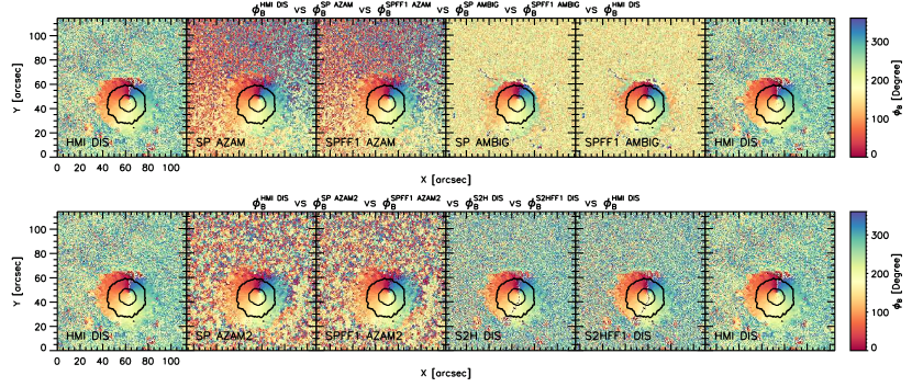
Figure 9.— Comparison between the azimuth disambiguated on HMI (explicitly denoted as HMI DIS) and SP using AZAM and AMBIG ($1^{st}\$row), and SP using AZAM2 and S2H using DIS ($2^{nd}\$row), for inversions considering FF variable (SP an S2H) and FF fixed to 1 (SPFF1 and S2HFF1).

Table 15Comparison between the spherical components of the vector magnetic field observed by HMI and SP, SP disambiguated with AZAM2, and with AMBIG.

$\mathbf{SolarFeature}$	$\mathbf{B^{\mathbf{HMI}}_{\mathbf{}}}$  vs $\mathbf{B^{\mathbf{SP}}_{\mathbf{}}}$	$\mathbf{<s_{e}>}$	$\mathbf{<r>}$	$\mathbf{<r^{2}>}$
Umbra	$|B|^{HMI}=(-0.11\pm 0.31)+(0.99\pm 0.12)\times|B|^{SP}$	$0.10\pm 0.03$	$0.92\pm 0.05$	$0.84\pm 0.09$
	$\theta_{B}^{HMI}=(12.60\pm 1.89)+(0.91\pm 0.01)\times\theta_{B}^{SP}$	$1.89\pm 0.57$	$0.99\pm 0.01$	$0.98\pm 0.02$
	$\phi_{B}^{HMI}=(14.77\pm 6.60)+(0.82\pm 0.08)\times\phi_{B}^{SP}$	$29.04\pm 5.67$	$0.77\pm 0.12$	$0.61\pm 0.18$
	$\phi_{B}^{HMI\ DIS}=(5.48\pm 10.49)+(0.97\pm 0.05)\times\phi_{B}^{SP\ AZAM}$	$19.11\pm 3.85$	$0.91\pm 0.04$	$0.83\pm 0.08$
	$\phi_{B}^{HMI\ DIS}=(6.65\pm 21.73)+(0.96\pm 0.10)\times\phi_{B}^{SP\ AZAM2}$	$20.18\pm 6.44$	$0.90\pm 0.07$	$0.82\pm 0.11$
	$\phi_{B}^{HMI\ DIS}=(13.06\pm 14.68)+(0.93\pm 0.07)\times\phi_{B}^{SP\ AMBIG}$	$20.88\pm 3.99$	$0.89\pm 0.06$	$0.80\pm 0.10$
Penumbra	$|B|^{HMI}=(0.01\pm 0.01)+(0.93\pm 0.02)\times|B|^{SP}$	$0.13\pm 0.02$	$0.96\pm 0.01$	$0.91\pm 0.02$
	$\theta_{B}^{HMI}=(14.37\pm 2.01)+(0.86\pm 0.02)\times\theta_{B}^{SP}$	$4.98\pm 0.40$	$0.97\pm 0.02$	$0.94\pm 0.03$
	$\phi_{B}^{HMI}=(13.00\pm 4.82)+(0.85\pm 0.04)\times\phi_{B}^{SP}$	$24.95\pm 2.49$	$0.87\pm 0.03$	$0.75\pm 0.05$
	$\phi_{B}^{HMI\ DIS}=(13.11\pm 6.93)+(0.92\pm 0.03)\times\phi_{B}^{SP\ AZAM}$	$36.28\pm 6.33$	$0.92\pm 0.03$	$0.85\pm 0.05$
	$\phi_{B}^{HMI\ DIS}=(13.44\pm 7.04)+(0.92\pm 0.03)\times\phi_{B}^{SP\ AZAM2}$	$36.88\pm 6.73$	$0.92\pm 0.03$	$0.84\pm 0.05$
	$\phi_{B}^{HMI\ DIS}=(13.58\pm 6.84)+(0.92\pm 0.03)\times\phi_{B}^{SP\ AMBIG}$	$37.17\pm 6.59$	$0.91\pm 0.03$	$0.84\pm 0.05$
Strong B Plage	$|B|^{HMI}=(0.19\pm 0.01)+(0.07\pm 0.03)\times|B|^{SP}$	$0.12\pm 0.01$	$0.16\pm 0.08$	$0.03\pm 0.03$
	$\theta_{B}^{HMI}=(56.19\pm 1.83)+(0.39\pm 0.02)\times\theta_{B}^{SP}$	$11.06\pm 0.77$	$0.83\pm 0.01$	$0.68\pm 0.02$
	$\phi_{B}^{HMI}=(52.10\pm 7.52)+(0.43\pm 0.09)\times\phi_{B}^{SP}$	$42.11\pm 2.15$	$0.46\pm 0.06$	$0.21\pm 0.06$
	$\phi_{B}^{HMI\ DIS}=(122.92\pm 7.75)+(0.45\pm 0.03)\times\phi_{B}^{SP\ AZAM}$	$82.86\pm 5.05$	$0.47\pm 0.04$	$0.22\pm 0.04$
	$\phi_{B}^{HMI\ DIS}=(125.45\pm 9.46)+(0.43\pm 0.03)\times\phi_{B}^{SP\ AZAM2}$	$83.71\pm 4.63$	$0.45\pm 0.04$	$0.21\pm 0.03$
	$\phi_{B}^{HMI\ DIS}=(112.48\pm 10.89)+(0.49\pm 0.04)\times\phi_{B}^{SP\ AMBIG}$	$84.97\pm 4.77$	$0.43\pm 0.04$	$0.18\pm 0.03$
Weak B Plage	$|B|^{HMI}=(0.13\pm 0.01)+(0.00\pm 0.01)\times|B|^{SP}$	$0.04\pm 0.00$	$0.01\pm 0.04$	$0.00\pm 0.00$
	$\theta_{B}^{HMI}=(62.72\pm 2.41)+(0.30\pm 0.02)\times\theta_{B}^{SP}$	$11.17\pm 0.97$	$0.78\pm 0.02$	$0.61\pm 0.03$
	$\phi_{B}^{HMI}=(72.95\pm 4.70)+(0.19\pm 0.03)\times\phi_{B}^{SP}$	$44.44\pm 0.88$	$0.20\pm 0.02$	$0.04\pm 0.01$
	$\phi_{B}^{HMI\ DIS}=(174.89\pm 9.38)+(0.23\pm 0.02)\times\phi_{B}^{SP\ AZAM}$	$85.83\pm 2.88$	$0.26\pm 0.02$	$0.07\pm 0.01$
	$\phi_{B}^{HMI\ DIS}=(179.99\pm 10.53)+(0.19\pm 0.03)\times\phi_{B}^{SP\ AZAM2}$	$86.63\pm 2.84$	$0.22\pm 0.03$	$0.05\pm 0.01$
	$\phi_{B}^{HMI\ DIS}=(195.01\pm 11.89)+(0.10\pm 0.05)\times\phi_{B}^{SP\ AMBIG}$	$88.48\pm 3.01$	$0.08\pm 0.04$	$0.01\pm 0.01$
$\mathbf{SolarFeature}$	$\mathbf{B^{\mathbf{HMI}}_{\mathbf{}}}$  vs $\mathbf{B^{\mathbf{SPFF1}}_{\mathbf{}}}$	$\mathbf{<s_{e}>}$	$\mathbf{<r>}$	$\mathbf{<r^{2}>}$
Umbra	$|B|^{HMI}=(-0.07\pm 0.21)+(0.98\pm 0.09)\times|B|^{SPFF1}$	$0.09\pm 0.03$	$0.92\pm 0.05$	$0.85\pm 0.08$
	$\theta_{B}^{HMI}=(10.79\pm 2.17)+(0.92\pm 0.01)\times\theta_{B}^{SPFF1}$	$1.84\pm 0.55$	$0.99\pm 0.01$	$0.98\pm 0.02$
	$\phi_{B}^{HMI}=(14.98\pm 6.84)+(0.81\pm 0.08)\times\phi_{B}^{SPFF1}$	$29.06\pm 5.83$	$0.77\pm 0.12$	$0.60\pm 0.19$
	$\phi_{B}^{HMI\ DIS}=(5.45\pm 9.98)+(0.97\pm 0.05)\times\phi_{B}^{SPFF1\ AZAM}$	$19.10\pm 3.83$	$0.91\pm 0.04$	$0.84\pm 0.07$
	$\phi_{B}^{HMI\ DIS}=(11.46\pm 18.91)+(0.94\pm 0.08)\times\phi_{B}^{SPFF1\ AZAM2}$	$21.31\pm 5.65$	$0.89\pm 0.06$	$0.80\pm 0.10$
	$\phi_{B}^{HMI\ DIS}=(13.06\pm 14.68)+(0.93\pm 0.07)\times\phi_{B}^{SPFF1\ AMBIG}$	$20.88\pm 3.99$	$0.89\pm 0.06$	$0.80\pm 0.10$
Penumbra	$|B|^{HMI}=(0.10\pm 0.02)+(0.92\pm 0.01)\times|B|^{SPFF1}$	$0.09\pm 0.01$	$0.98\pm 0.01$	$0.96\pm 0.01$
	$\theta_{B}^{HMI}=(11.14\pm 2.27)+(0.90\pm 0.02)\times\theta_{B}^{SPFF1}$	$4.56\pm 0.41$	$0.97\pm 0.01$	$0.95\pm 0.03$
	$\phi_{B}^{HMI}=(12.70\pm 4.82)+(0.86\pm 0.04)\times\phi_{B}^{SPFF1}$	$24.57\pm 2.76$	$0.87\pm 0.03$	$0.76\pm 0.05$
	$\phi_{B}^{HMI\ DIS}=(13.50\pm 6.67)+(0.92\pm 0.03)\times\phi_{B}^{SPFF1\ AZAM}$	$36.83\pm 6.26$	$0.92\pm 0.03$	$0.84\pm 0.05$
	$\phi_{B}^{HMI\ DIS}=(13.82\pm 6.89)+(0.92\pm 0.03)\times\phi_{B}^{SPFF1\ AZAM2}$	$37.38\pm 6.56$	$0.91\pm 0.03$	$0.84\pm 0.05$
	$\phi_{B}^{HMI\ DIS}=(13.58\pm 6.84)+(0.92\pm 0.03)\times\phi_{B}^{SPFF1\ AMBIG}$	$37.17\pm 6.59$	$0.91\pm 0.03$	$0.84\pm 0.05$
Strong B Plage	$|B|^{HMI}=(0.17\pm 0.01)+(0.35\pm 0.06)\times|B|^{SPFF1}$	$0.11\pm 0.01$	$0.49\pm 0.07$	$0.25\pm 0.07$
	$\theta_{B}^{HMI}=(32.38\pm 3.30)+(0.65\pm 0.04)\times\theta_{B}^{SPFF1}$	$9.14\pm 1.01$	$0.91\pm 0.01$	$0.82\pm 0.03$
	$\phi_{B}^{HMI}=(35.82\pm 8.28)+(0.60\pm 0.09)\times\phi_{B}^{SPFF1}$	$37.83\pm 3.97$	$0.63\pm 0.07$	$0.40\pm 0.09$
	$\phi_{B}^{HMI\ DIS}=(75.07\pm 11.34)+(0.63\pm 0.06)\times\phi_{B}^{SPFF1\ AZAM}$	$74.13\pm 7.92$	$0.64\pm 0.07$	$0.41\pm 0.09$
	$\phi_{B}^{HMI\ DIS}=(78.54\pm 8.88)+(0.61\pm 0.03)\times\phi_{B}^{SPFF1\ AZAM2}$	$75.19\pm 5.68$	$0.63\pm 0.03$	$0.39\pm 0.04$
	$\phi_{B}^{HMI\ DIS}=(76.08\pm 9.66)+(0.62\pm 0.05)\times\phi_{B}^{SPFF1\ AMBIG}$	$77.70\pm 6.27$	$0.59\pm 0.04$	$0.35\pm 0.05$
Weak B Plage	$|B|^{HMI}=(0.12\pm 0.01)+(0.10\pm 0.01)\times|B|^{SPFF1}$	$0.05\pm 0.00$	$0.19\pm 0.03$	$0.04\pm 0.01$
	$\theta_{B}^{HMI}=(51.79\pm 2.84)+(0.42\pm 0.03)\times\theta_{B}^{SPFF1}$	$11.29\pm 0.98$	$0.79\pm 0.02$	$0.62\pm 0.03$
	$\phi_{B}^{HMI}=(70.08\pm 5.61)+(0.22\pm 0.04)\times\phi_{B}^{SPFF1}$	$44.30\pm 1.11$	$0.24\pm 0.03$	$0.06\pm 0.01$
	$\phi_{B}^{HMI\ DIS}=(171.25\pm 9.31)+(0.24\pm 0.02)\times\phi_{B}^{SPFF1\ AZAM}$	$86.60\pm 3.05$	$0.26\pm 0.02$	$0.07\pm 0.01$
	$\phi_{B}^{HMI\ DIS}=(175.75\pm 9.34)+(0.20\pm 0.02)\times\phi_{B}^{SPFF1\ AZAM2}$	$87.30\pm 2.99$	$0.23\pm 0.02$	$0.05\pm 0.01$
	$\phi_{B}^{HMI\ DIS}=(189.29\pm 11.56)+(0.12\pm 0.05)\times\phi_{B}^{SPFF1\ AMBIG}$	$89.24\pm 3.13$	$0.10\pm 0.04$	$0.01\pm 0.01$

Table 16Comparison between the spherical components of the vector magnetic field observed by HMI and S2H, HMI and S2H disambiguated by DIS, and the corresponding comparisons for S2H with FF=1 (S2HFF1).

$\mathbf{SolarFeature}$	$\mathbf{B^{\mathbf{HMI}}_{\mathbf{}}}$  vs $\mathbf{B^{\mathbf{S2H}}_{\mathbf{}}}$	$\mathbf{<s_{e}>}$	$\mathbf{<r>}$	$\mathbf{<r^{2}>}$
Umbra	$|B|^{HMI}=(0.23\pm 0.18)+(0.85\pm 0.07)\times|B|^{S2H}$	$0.10\pm 0.02$	$0.91\pm 0.04$	$0.84\pm 0.07$
	$\theta_{B}^{HMI}=(13.57\pm 2.28)+(0.89\pm 0.02)\times\theta_{B}^{S2H}$	$2.03\pm 0.52$	$0.99\pm 0.01$	$0.98\pm 0.02$
	$\phi_{B}^{HMI}=(16.30\pm 6.50)+(0.79\pm 0.08)\times\phi_{B}^{S2H}$	$30.40\pm 5.28$	$0.75\pm 0.12$	$0.57\pm 0.19$
	$\phi_{B}^{HMI\ DIS}=(67.98\pm 50.21)+(0.67\pm 0.20)\times\phi_{B}^{S2H\ DIS}$	$25.27\pm 3.31$	$0.84\pm 0.07$	$0.71\pm 0.11$
Penumbra	$|B|^{HMI}=(0.01\pm 0.02)+(0.98\pm 0.02)\times|B|^{S2H}$	$0.11\pm 0.01$	$0.97\pm 0.01$	$0.95\pm 0.01$
	$\theta_{B}^{HMI}=(11.39\pm 2.56)+(0.90\pm 0.02)\times\theta_{B}^{S2H}$	$4.62\pm 0.52$	$0.97\pm 0.02$	$0.95\pm 0.03$
	$\phi_{B}^{HMI}=(10.78\pm 4.47)+(0.88\pm 0.04)\times\phi_{B}^{S2H}$	$23.36\pm 3.69$	$0.88\pm 0.04$	$0.78\pm 0.06$
	$\phi_{B}^{HMI\ DIS}=(8.39\pm 4.99)+(0.95\pm 0.02)\times\phi_{B}^{S2H\ DIS}$	$25.11\pm 3.98$	$0.96\pm 0.01$	$0.93\pm 0.02$
Strong B Plage	$|B|^{HMI}=(0.19\pm 0.01)+(0.13\pm 0.02)\times|B|^{S2H}$	$0.12\pm 0.01$	$0.28\pm 0.05$	$0.08\pm 0.03$
	$\theta_{B}^{HMI}=(47.78\pm 2.67)+(0.48\pm 0.03)\times\theta_{B}^{S2H}$	$10.89\pm 0.82$	$0.84\pm 0.01$	$0.71\pm 0.02$
	$\phi_{B}^{HMI}=(47.55\pm 8.57)+(0.47\pm 0.09)\times\phi_{B}^{S2H}$	$41.44\pm 2.67$	$0.50\pm 0.07$	$0.25\pm 0.07$
	$\phi_{B}^{HMI\ DIS}=(37.81\pm 7.52)+(0.81\pm 0.03)\times\phi_{B}^{S2H\ DIS}$	$50.63\pm 5.02$	$0.85\pm 0.02$	$0.72\pm 0.04$
Weak B Plage	$|B|^{HMI}=(0.14\pm 0.01)(-0.00\pm 0.01)\times|B|^{S2H}$	$0.05\pm 0.00$	$-0.01\pm 0.03$	$0.00\pm 0.00$
	$\theta_{B}^{HMI}=(54.02\pm 2.97)+(0.40\pm 0.03)\times\theta_{B}^{S2H}$	$11.34\pm 1.00$	$0.78\pm 0.02$	$0.61\pm 0.03$
	$\phi_{B}^{HMI}=(72.72\pm 5.15)+(0.18\pm 0.03)\times\phi_{B}^{S2H}$	$44.61\pm 1.04$	$0.20\pm 0.02$	$0.04\pm 0.01$
	$\phi_{B}^{HMI\ DIS}=(66.67\pm 9.49)+(0.69\pm 0.03)\times\phi_{B}^{S2H\ DIS}$	$59.83\pm 3.12$	$0.74\pm 0.02$	$0.55\pm 0.04$
$\mathbf{SolarFeature}$	$\mathbf{B^{\mathbf{HMI}}_{\mathbf{}}}$  vs $\mathbf{B^{\mathbf{S2HFF1}}_{\mathbf{}}}$	$\mathbf{<s_{e}>}$	$\mathbf{<r>}$	$\mathbf{<r^{2}>}$
Umbra	$|B|^{HMI}=(0.25\pm 0.15)+(0.85\pm 0.06)\times|B|^{S2HFF1}$	$0.08\pm 0.02$	$0.94\pm 0.04$	$0.88\pm 0.06$
	$\theta_{B}^{HMI}=(12.69\pm 2.93)+(0.90\pm 0.02)\times\theta_{B}^{S2HFF1}$	$1.99\pm 0.56$	$0.99\pm 0.01$	$0.98\pm 0.02$
	$\phi_{B}^{HMI}=(16.15\pm 6.75)+(0.80\pm 0.08)\times\phi_{B}^{S2HFF1}$	$30.24\pm 5.78$	$0.75\pm 0.12$	$0.58\pm 0.18$
	$\phi_{B}^{HMI\ DIS}=(68.01\pm 48.61)+(0.67\pm 0.19)\times\phi_{B}^{S2HFF1\ DIS}$	$25.41\pm 4.22$	$0.84\pm 0.07$	$0.71\pm 0.11$
Penumbra	$|B|^{HMI}=(0.04\pm 0.01)+(0.96\pm 0.01)\times|B|^{S2HFF1}$	$0.09\pm 0.01$	$0.98\pm 0.00$	$0.97\pm 0.01$
	$\theta_{B}^{HMI}=(10.31\pm 2.51)+(0.91\pm 0.02)\times\theta_{B}^{S2HFF1}$	$4.50\pm 0.47$	$0.97\pm 0.01$	$0.95\pm 0.03$
	$\phi_{B}^{HMI}=(10.46\pm 4.22)+(0.88\pm 0.04)\times\phi_{B}^{S2HFF1}$	$23.22\pm 3.69$	$0.88\pm 0.04$	$0.78\pm 0.06$
	$\phi_{B}^{HMI\ DIS}=(8.23\pm 4.56)+(0.95\pm 0.02)\times\phi_{B}^{S2HFF1\ DIS}$	$25.00\pm 3.95$	$0.96\pm 0.01$	$0.93\pm 0.02$
Strong B Plage	$|B|^{HMI}=(0.15\pm 0.01)+(0.41\pm 0.05)\times|B|^{S2HFF1}$	$0.10\pm 0.01$	$0.53\pm 0.06$	$0.28\pm 0.06$
	$\theta_{B}^{HMI}=(30.68\pm 4.33)+(0.67\pm 0.05)\times\theta_{B}^{S2HFF1}$	$9.38\pm 1.07$	$0.90\pm 0.01$	$0.81\pm 0.03$
	$\phi_{B}^{HMI}=(39.12\pm 9.12)+(0.56\pm 0.09)\times\phi_{B}^{S2HFF1}$	$39.62\pm 3.77$	$0.58\pm 0.08$	$0.34\pm 0.09$
	$\phi_{B}^{HMI\ DIS}=(29.07\pm 6.71)+(0.85\pm 0.03)\times\phi_{B}^{S2HFF1\ DIS}$	$46.70\pm 5.81$	$0.87\pm 0.02$	$0.76\pm 0.04$
Weak B Plage	$|B|^{HMI}=(0.12\pm 0.01)+(0.09\pm 0.01)\times|B|^{S2HFF1}$	$0.05\pm 0.00$	$0.16\pm 0.04$	$0.03\pm 0.01$
	$\theta_{B}^{HMI}=(43.64\pm 3.57)+(0.52\pm 0.04)\times\theta_{B}^{S2HFF1}$	$10.72\pm 1.10$	$0.81\pm 0.02$	$0.66\pm 0.03$
	$\phi_{B}^{HMI}=(72.06\pm 5.52)+(0.19\pm 0.04)\times\phi_{B}^{S2HFF1}$	$44.65\pm 1.11$	$0.21\pm 0.03$	$0.04\pm 0.01$
	$\phi_{B}^{HMI\ DIS}=(65.55\pm 8.87)+(0.69\pm 0.03)\times\phi_{B}^{S2HFF1\ DIS}$	$59.79\pm 3.07$	$0.74\pm 0.02$	$0.55\pm 0.03$

Figure 9 shows the azimuth disambiguated for HMI in the $1^{st}\$and $6^{th}$ column in both rows. We have explicitly denoted the disambiguated azimuth observed by HMI as ‘HMI DIS’. In the $2^{nd}\$and $3^{rd}\$images of the $1^{st}\$row, we show the disambiguated azimuth for SP and SFFF1. The same azimuth values disambiguated with AMBIG are shown in the $4^{th}$ and $5^{th}$ images. In the $2^{nd}\$row, the $2^{nd}\$and $3^{rd}\$maps are showing the disambiguated SP and SPFF1 azimuth with AZAM2, and the $4^{th}$ and $5^{th}$ images show S2H and S2HFF1 azimuth disambiguated as HMI does, therefore, they are also denoted with ‘DIS’. At a glance, it is clear that different disambiguation codes may give slightly different solutions to the ambiguty of the azimuth (SP AZAM vs SP AZAM2), or quite different solutions (SP AZAM or AZAM2 vs SP AMBIG), even when the codes are working on the same data (azimuth of SP data). This difference is most noticeable in the plage. The solution found by the same code (DIS) applied to similar data (S2H and HMI) gives a close solution between those data set. The statistical values of this visual comparison are given in Table 15 and 16. The ${<}b{>}\$for the relationship between the disambiguated azimuths $\phi_{B}^{HMIDIS}$ and $\phi_{B}^{S2HDIS}$ in the weak and strong plage are as high as $\sim 0.8$ and $0.6$ respectively, showing a moderately strong correlation (${<}r{>}\$$\sim 0.85$ and $0.75$ respectively). However, it would be a mistake to considerer a solution to be the ‘right solution’ because of these high values in the correlation between of the azimuths. Since, what these statistical values tell us is that the solution for the ambiguity in the azimuth for the data compared is very close, if not the same, in both data set. We conclude that using different methods for the same data set may provide different solutions (e.g. AZAM vs AMBIG on SP data), but using similar methods with similar data set provides similar solutions (SP AZAM vs SP AZAM2 or HMI DIS vs S2H DIS).

Table 17 shows the results for the straightforward comparison between HMI and SP, being SP disambiguated with the methods mentioned above. Again, for a better comparison we keep the results showed in Table 3 as the $1^{st}\$sub-table. The $2^{nd}\$and $3^{rd}\$sub-tables show the same comparison between the components of the magnetic field observed by HMI and the ones observed by SP when they have been disambiguated with the methods ii) and iii) respectively. The results for the three disambiguation methods are statistically similar in all the RoIs. That means, to apply these other disambiguation methods to SP data does not have an impact in the comparison with HMI disambiguated data. Figure 10 shows the same maps that Fig. 4, but here they are disambiguated with method AZAM2 (top panels) and AMBIG (bottom panels). The maps in Fig. 10 show a more coherent spatial distribution of the values than for the maps in Fig. 4. However, this fact has not an impact in the statistical values for the comparison of the components of the vector magnetic field, since most of the pixels showing that different solution are not considered in the comparison, not even as part of the weak plage, because their polarization signal is below the criteria used in this paper (see Section 2.2).

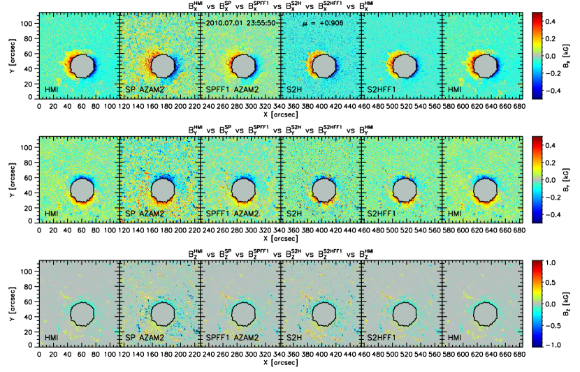
Figure 10.— Components of the Cartesian components of the vector magnetic field observed by HMI ($1^{st}\$column), SP ($2^{nd}\$column), SP with FF=1 ($3^{rd}\$column), S2H ($4^{th}$ column), S2H with FF=1 ($5^{th}$ column), and, for making the visual comparison easier to the reader, again HMI ($6^{th}$ column) in the sunspot ($1^{st}\$to $3^{rd}\$row) and the plage ($4^{th}$ to $6^{th}$. Top: maps disambiguated using AZAM2. Bottom: maps disambguated using AMBIG.

Table 17Comparison between the Cartesian components of the vector magnetic field observed by HMI and SP, and SP disambiguated with the AZAM2, and with AMBIG.

$\mathbf{Solar\ Feature}$	$\mathbf{B^{\mathbf{HMI}}_{\mathbf{}}}$  vs $\mathbf{B^{\mathbf{SP}}_{\mathbf{}}}$	$\mathbf{<s_{e}>}$	$\mathbf{<r>}$	$\mathbf{<r^{2}>}$
Umbra	$B^{HMI}_{X}=(+0.05\pm 0.10)+(+0.99\pm 0.02)\times B^{SP}_{X}$	$0.09\pm 0.02$	$0.99\pm 0.00$	$0.99\pm 0.01$
	$B^{HMI}_{Y}=(-0.00\pm 0.04)+(+0.98\pm 0.02)\times B^{SP}_{Y}$	$0.09\pm 0.02$	$0.99\pm 0.00$	$0.98\pm 0.01$
	$B^{HMI}_{Z}=(-0.23\pm 0.10)+(+0.82\pm 0.06)\times B^{SP}_{Z}$	$0.10\pm 0.03$	$0.96\pm 0.02$	$0.93\pm 0.04$
Penumbra	$B^{HMI}_{X}=(+0.00\pm 0.01)+(+0.97\pm 0.02)\times B^{SP}_{X}$	$0.10\pm 0.01$	$0.99\pm 0.00$	$0.98\pm 0.01$
	$B^{HMI}_{Y}=(+0.01\pm 0.01)+(+0.95\pm 0.02)\times B^{SP}_{Y}$	$0.11\pm 0.02$	$0.99\pm 0.00$	$0.97\pm 0.01$
	$B^{HMI}_{Z}=(-0.02\pm 0.01)+(+0.84\pm 0.05)\times B^{SP}_{Z}$	$0.11\pm 0.01$	$0.97\pm 0.01$	$0.94\pm 0.01$
Strong B Plage	$B^{HMI}_{X}=(-0.03\pm 0.01)+(+0.40\pm 0.11)\times B^{SP}_{X}$	$0.16\pm 0.02$	$0.65\pm 0.12$	$0.44\pm 0.14$
	$B^{HMI}_{Y}=(+0.02\pm 0.01)+(+0.33\pm 0.08)\times B^{SP}_{Y}$	$0.16\pm 0.01$	$0.59\pm 0.10$	$0.35\pm 0.12$
	$B^{HMI}_{Z}=(-0.01\pm 0.01)+(+0.15\pm 0.01)\times B^{SP}_{Z}$	$0.07\pm 0.01$	$0.72\pm 0.02$	$0.52\pm 0.04$
Weak B Plage	$B^{HMI}_{X}=(-0.02\pm 0.01)+(+0.21\pm 0.04)\times B^{SP}_{X}$	$0.10\pm 0.01$	$0.40\pm 0.05$	$0.17\pm 0.04$
	$B^{HMI}_{Y}=(+0.01\pm 0.01)+(+0.17\pm 0.04)\times B^{SP}_{Y}$	$0.10\pm 0.00$	$0.36\pm 0.05$	$0.14\pm 0.04$
	$B^{HMI}_{Z}=(-0.01\pm 0.00)+(+0.10\pm 0.02)\times B^{SP}_{Z}$	$0.05\pm 0.00$	$0.63\pm 0.03$	$0.40\pm 0.04$
$\mathbf{Solar\ Feature}$	$\mathbf{B^{\mathbf{HMI}}_{\mathbf{}}}$  vs $\mathbf{B^{\mathbf{SP\ AZAM2}}_{\mathbf{}}}$	$\mathbf{<s_{e}>}$	$\mathbf{<r>}$	$\mathbf{<r^{2}>}$
Umbra	$B^{HMI}_{X}=(+0.05\pm 0.10)+(+0.99\pm 0.02)\times B^{SP}_{X}$	$0.09\pm 0.02$	$0.99\pm 0.00$	$0.99\pm 0.01$
	$B^{HMI}_{Y}=(-0.00\pm 0.04)+(+0.97\pm 0.02)\times B^{SP}_{Y}$	$0.10\pm 0.03$	$0.99\pm 0.00$	$0.98\pm 0.01$
	$B^{HMI}_{Z}=(-0.23\pm 0.10)+(+0.82\pm 0.06)\times B^{SP}_{Z}$	$0.10\pm 0.03$	$0.96\pm 0.02$	$0.93\pm 0.04$
Penumbra	$B^{HMI}_{X}=(+0.00\pm 0.01)+(+0.97\pm 0.02)\times B^{SP}_{X}$	$0.11\pm 0.02$	$0.99\pm 0.00$	$0.98\pm 0.01$
	$B^{HMI}_{Y}=(+0.01\pm 0.01)+(+0.95\pm 0.02)\times B^{SP}_{Y}$	$0.11\pm 0.02$	$0.99\pm 0.00$	$0.97\pm 0.01$
	$B^{HMI}_{Z}=(-0.02\pm 0.01)+(+0.84\pm 0.05)\times B^{SP}_{Z}$	$0.11\pm 0.01$	$0.97\pm 0.01$	$0.94\pm 0.01$
Strong B Plage	$B^{HMI}_{X}=(-0.03\pm 0.02)+(+0.39\pm 0.11)\times B^{SP}_{X}$	$0.17\pm 0.02$	$0.63\pm 0.11$	$0.41\pm 0.14$
	$B^{HMI}_{Y}=(+0.02\pm 0.02)+(+0.32\pm 0.07)\times B^{SP}_{Y}$	$0.16\pm 0.01$	$0.58\pm 0.09$	$0.34\pm 0.10$
	$B^{HMI}_{Z}=(-0.01\pm 0.01)+(+0.15\pm 0.01)\times B^{SP}_{Z}$	$0.07\pm 0.01$	$0.72\pm 0.02$	$0.52\pm 0.04$
Weak B Plage	$B^{HMI}_{X}=(-0.02\pm 0.01)+(+0.18\pm 0.04)\times B^{SP}_{X}$	$0.10\pm 0.01$	$0.36\pm 0.04$	$0.13\pm 0.03$
	$B^{HMI}_{Y}=(+0.01\pm 0.01)+(+0.16\pm 0.03)\times B^{SP}_{Y}$	$0.10\pm 0.00$	$0.35\pm 0.04$	$0.12\pm 0.03$
	$B^{HMI}_{Z}=(-0.01\pm 0.00)+(+0.10\pm 0.02)\times B^{SP}_{Z}$	$0.05\pm 0.00$	$0.63\pm 0.03$	$0.40\pm 0.04$
$\mathbf{Solar\ Feature}$	$\mathbf{B^{\mathbf{HMI}}_{\mathbf{}}}$  vs $\mathbf{B^{\mathbf{SP\ AMBIG}}_{\mathbf{}}}$	$\mathbf{<s_{e}>}$	$\mathbf{<r>}$	$\mathbf{<r^{2}>}$
Umbra	$B^{HMI}_{X}=(+0.05\pm 0.10)+(+0.99\pm 0.02)\times B^{SP}_{X}$	$0.09\pm 0.02$	$0.99\pm 0.00$	$0.99\pm 0.01$
	$B^{HMI}_{Y}=(-0.00\pm 0.04)+(+0.98\pm 0.02)\times B^{SP}_{Y}$	$0.09\pm 0.02$	$0.99\pm 0.00$	$0.98\pm 0.01$
	$B^{HMI}_{Z}=(-0.23\pm 0.10)+(+0.82\pm 0.06)\times B^{SP}_{Z}$	$0.10\pm 0.03$	$0.96\pm 0.02$	$0.93\pm 0.04$
Penumbra	$B^{HMI}_{X}=(+0.00\pm 0.01)+(+0.97\pm 0.02)\times B^{SP}_{X}$	$0.10\pm 0.01$	$0.99\pm 0.00$	$0.98\pm 0.01$
	$B^{HMI}_{Y}=(+0.01\pm 0.01)+(+0.95\pm 0.02)\times B^{SP}_{Y}$	$0.11\pm 0.02$	$0.99\pm 0.00$	$0.97\pm 0.01$
	$B^{HMI}_{Z}=(-0.02\pm 0.01)+(+0.84\pm 0.05)\times B^{SP}_{Z}$	$0.11\pm 0.01$	$0.97\pm 0.01$	$0.94\pm 0.01$
Strong B Plage	$B^{HMI}_{X}=(-0.02\pm 0.01)+(+0.39\pm 0.08)\times B^{SP}_{X}$	$0.17\pm 0.01$	$0.65\pm 0.06$	$0.42\pm 0.07$
	$B^{HMI}_{Y}=(-0.01\pm 0.01)+(+0.36\pm 0.07)\times B^{SP}_{Y}$	$0.16\pm 0.00$	$0.61\pm 0.07$	$0.38\pm 0.09$
	$B^{HMI}_{Z}=(-0.01\pm 0.01)+(+0.15\pm 0.01)\times B^{SP}_{Z}$	$0.07\pm 0.01$	$0.72\pm 0.02$	$0.52\pm 0.04$
Weak B Plage	$B^{HMI}_{X}=(-0.02\pm 0.01)+(+0.14\pm 0.02)\times B^{SP}_{X}$	$0.10\pm 0.01$	$0.28\pm 0.04$	$0.08\pm 0.02$
	$B^{HMI}_{Y}=(+0.00\pm 0.01)+(+0.14\pm 0.03)\times B^{SP}_{Y}$	$0.10\pm 0.00$	$0.29\pm 0.03$	$0.08\pm 0.02$
	$B^{HMI}_{Z}=(-0.01\pm 0.00)+(+0.10\pm 0.02)\times B^{SP}_{Z}$	$0.05\pm 0.00$	$0.63\pm 0.03$	$0.40\pm 0.04$

However, as we pointed out in Section 3.1, there are regions where the horizontal components of the vector magnetic field observed by HMI show opposite (or mixed) polarity with respect to the ones observed by SP. We have studied in how many pixels in the comparison between HMI and SP that happens. Since the three disambiguations methods provide statistically the same results for the umbra and the penumbra (see Table 17), we only offer the results for the strong and weak plage in the following tables. Tables 18, 19, and 20 are divided as follows. In the top of these tables, there is the comparison between the HMI and SP/SPFF1 without considering any relationship between the sign of the components, as it has been done in the main body of the paper (e.g., the sub-table in the top of 18 is the same that 3). In the middle and the bottom of these tables, we have done the same analysis, i.e., linear regression fit and averaged statistical values for the components of the magnetic field observed by two data set at the pixels showing a positive relationship (middle sub-table) and a negative relationship (bottom sub-table) between their horizontal components. In addition, in these tables we show the percentage of the pixels evaluated in the comparison. For the sub-table in the top, the percentages refer to the total size of the map, while for the sub-tables in the middle and the bottom they refer to the size of the RoI considered. Table 18 refers to the straightforward comparison between $\mathbf{B^{\mathbf{HMI}}_{\mathbf{}}}$  and $\mathbf{B^{\mathbf{SP}}_{\mathbf{}}}$ , i.e., as it is considered in Section 3.1. We have done a similar analysis for the comparison between HMI and SP data disambiguated with AZAM method ii) and with AMBIG code. For the three disambiguation methods used in this paper, the percentages of pixels having the same sign for the horizontal components of the magnetic field are very similar in the three tables, either for the strong plage ($73-80\%$) or the weak plage ($61-67\%$). The number of pixels with opposite sign in the comparison is, although calculated independently, the complementary to $100\%$ of those values. That happens even when we consider the same data, from the same instrument (same spatial and spectral sampling, same spectral line) and solved with the same inversion code (IC) as it is showed in Table 20, where we compare $\mathbf{B^{\mathbf{SP\ AMBIG}}_{\mathbf{}}}$  with $\mathbf{B^{\mathbf{SP}}_{\mathbf{}}}$ . Because of all the results are similar in the three cases, we conclude that the different disambiguation solutions used in this study - AZAM methods i) and ii) and AMBIG - introduce a change of sign in the solar structures with respect to the solution found by HMI observed about $\sim 25\%$ in the strong plage, and about $\sim 35\%$ in the weak plage.

It is obvious that disentangling the mixed sings favor a better linear relationship between the horizontal components. If we would only consider those pixels where the relationship of the horizontal component is positive – i.e., the solutions of disambiguation methods used here match with the one found by HMI–, all the averaged statistical values ${<}s_{e}{>}\$, ${<}r{>}\$, and ${<}r^{2}{>}\$will have a significant improvement, both in the strong and the weak plage. Table 19 compares the HMI data with the SP data inverted considering a FF fixed to 1. The correlation for between the horizontal components in those pixels sharing the same sign in both maps become ${<}r{>}\$$\sim 0.92$ and $\sim 83$ for the strong and the weak plage.

The values associate to the Y component of the vector magnetic field is the one showing the biggest improvement. As we explained in Section 3.2, there are several solar structures in the $\mathbf{B^{\mathbf{HMI}}_{\mathbf{Y}}}$  maps of the plage showing opposite or mixed sign with respect the SP or pseudo-SP maps (see Figure 4). In summary, if we do not consider those structures the linear relationship between HMI and SP will become stronger. Applying a reliable disambiguation code able to solve the azimuth ambiguity to both HMI and SP data, would benefit the comparison between them. Of course, the solution found for such a code will rely on the azimuth found by the inversions results, but using the same disambiguation code might favor to find similar disambiguation solutions.

Table 18Comparison between the Cartesian components of the vector magnetic field observed by HMI and SP taking into account the sign between the horizontal components.

$\mathbf{SolarFeature}$	$\mathbf{B^{\mathbf{HMI}}_{\mathbf{}}}$  vs $\mathbf{B^{\mathbf{SP}}_{\mathbf{}}}$  Original	$\mathbf{<\sigma>}$	$\mathbf{<r>}$	$\mathbf{<r^{2}>}$	% Eval.
Strong B Plage	$B^{HMI}_{X}=(-0.03\pm 0.01)+(+0.40\pm 0.11)\times B^{SP}_{X}$	$0.16\pm 0.02$	$+0.65\pm 0.12$	$0.44\pm 0.14$	$4\pm 0$
	$B^{HMI}_{Y}=(+0.02\pm 0.01)+(+0.33\pm 0.08)\times B^{SP}_{Y}$	$0.16\pm 0.01$	$+0.59\pm 0.10$	$0.35\pm 0.12$	$4\pm 0$
	$B^{HMI}_{Z}=(-0.01\pm 0.01)+(+0.15\pm 0.01)\times B^{SP}_{Z}$	$0.07\pm 0.01$	$+0.72\pm 0.02$	$0.52\pm 0.04$	$4\pm 0$
Weak B Plage	$B^{HMI}_{X}=(-0.02\pm 0.01)+(+0.21\pm 0.04)\times B^{SP}_{X}$	$0.10\pm 0.01$	$+0.40\pm 0.05$	$0.17\pm 0.04$	$6\pm 0$
	$B^{HMI}_{Y}=(+0.01\pm 0.01)+(+0.17\pm 0.04)\times B^{SP}_{Y}$	$0.10\pm 0.00$	$+0.36\pm 0.05$	$0.14\pm 0.04$	$6\pm 1$
	$B^{HMI}_{Z}=(-0.01\pm 0.00)+(+0.10\pm 0.02)\times B^{SP}_{Z}$	$0.05\pm 0.00$	$+0.63\pm 0.03$	$0.40\pm 0.04$	$9\pm 1$
$\mathbf{SolarFeature}$	$\mathbf{B^{\mathbf{HMI}}_{\mathbf{}}}$  vs $\mathbf{B^{\mathbf{SP}}_{\mathbf{}}}$  Same Sign in XY (Pos.)	$\mathbf{<\sigma>}$	$\mathbf{<r>}$	$\mathbf{<r^{2}>}$	% Pos.
Strong B Plage	$B^{HMI}_{X}=(-0.01\pm 0.01)+(+0.55\pm 0.08)\times B^{SP}_{X}$	$0.12\pm 0.01$	$+0.86\pm 0.03$	$0.74\pm 0.05$	$80\pm 4$
	$B^{HMI}_{Y}=(+0.01\pm 0.01)+(+0.50\pm 0.05)\times B^{SP}_{Y}$	$0.12\pm 0.00$	$+0.84\pm 0.03$	$0.71\pm 0.05$	$77\pm 5$
	$B^{HMI}_{Z}=(-0.01\pm 0.01)+(+0.15\pm 0.01)\times B^{SP}_{Z}$	$0.07\pm 0.01$	$+0.74\pm 0.02$	$0.54\pm 0.03$	$95\pm 1$
Weak B Plage	$B^{HMI}_{X}=(-0.00\pm 0.00)+(+0.41\pm 0.06)\times B^{SP}_{X}$	$0.08\pm 0.01$	$+0.76\pm 0.03$	$0.58\pm 0.05$	$67\pm 3$
	$B^{HMI}_{Y}=(+0.01\pm 0.01)+(+0.37\pm 0.04)\times B^{SP}_{Y}$	$0.07\pm 0.00$	$+0.75\pm 0.02$	$0.56\pm 0.04$	$67\pm 2$
	$B^{HMI}_{Z}=(-0.01\pm 0.00)+(+0.11\pm 0.02)\times B^{SP}_{Z}$	$0.05\pm 0.00$	$+0.65\pm 0.03$	$0.42\pm 0.04$	$94\pm 1$
$\mathbf{SolarFeature}$	$\mathbf{B^{\mathbf{HMI}}_{\mathbf{}}}$  vs $\mathbf{B^{\mathbf{SP}}_{\mathbf{}}}$  Opposite Sign in XY (Neg.)	$\mathbf{<\sigma>}$	$\mathbf{<r>}$	$\mathbf{<r^{2}>}$	% Neg.
Strong B Plage	$B^{HMI}_{X}=(+0.00\pm 0.02)+(-0.29\pm 0.04)\times B^{SP}_{X}$	$0.08\pm 0.01$	$-0.73\pm 0.11$	$0.54\pm 0.14$	$20\pm 4$
	$B^{HMI}_{Y}=(-0.01\pm 0.01)+(-0.28\pm 0.03)\times B^{SP}_{Y}$	$0.08\pm 0.01$	$-0.78\pm 0.03$	$0.61\pm 0.05$	$23\pm 5$
	$B^{HMI}_{Z}=(-0.00\pm 0.00)+(-0.02\pm 0.01)\times B^{SP}_{Z}$	$0.02\pm 0.01$	$-0.48\pm 0.10$	$0.24\pm 0.09$	$5\pm 1$
Weak B Plage	$B^{HMI}_{X}=(-0.02\pm 0.01)+(-0.26\pm 0.04)\times B^{SP}_{X}$	$0.07\pm 0.00$	$-0.59\pm 0.05$	$0.35\pm 0.06$	$33\pm 3$
	$B^{HMI}_{Y}=(+0.00\pm 0.01)+(-0.27\pm 0.04)\times B^{SP}_{Y}$	$0.06\pm 0.00$	$-0.70\pm 0.03$	$0.48\pm 0.04$	$33\pm 2$
	$B^{HMI}_{Z}=(-0.00\pm 0.00)+(-0.03\pm 0.01)\times B^{SP}_{Z}$	$0.02\pm 0.00$	$-0.30\pm 0.05$	$0.09\pm 0.03$	$6\pm 1$

Table 19Comparison between the Cartesian components of the vector magnetic field observed by HMI and SPFF1 taking into account the sign between the horizontal components.

$\mathbf{SolarFeature}$	$\mathbf{B^{\mathbf{HMI}}_{\mathbf{}}}$  vs $\mathbf{B^{\mathbf{SPFF1}}_{\mathbf{}}}$  Original	$\mathbf{<s_{e}>}$	$\mathbf{<r>}$	$\mathbf{<r^{2}>}$	% Eval.
Strong B Plage	$B^{HMI}_{X}=(-0.01\pm 0.01)+(+0.74\pm 0.17)\times B^{SPFF1}_{X}$	$0.16\pm 0.04$	$+0.78\pm 0.14$	$0.62\pm 0.19$	$2\pm 0$
	$B^{HMI}_{Y}=(+0.01\pm 0.02)+(+0.66\pm 0.12)\times B^{SPFF1}_{Y}$	$0.17\pm 0.02$	$+0.74\pm 0.10$	$0.55\pm 0.14$	$2\pm 0$
	$B^{HMI}_{Z}=(-0.02\pm 0.01)+(+0.39\pm 0.05)\times B^{SPFF1}_{Z}$	$0.09\pm 0.01$	$+0.84\pm 0.02$	$0.71\pm 0.04$	$1\pm 0$
Weak B Plage	$B^{HMI}_{X}=(-0.02\pm 0.01)+(+0.50\pm 0.08)\times B^{SPFF1}_{X}$	$0.10\pm 0.01$	$+0.50\pm 0.06$	$0.26\pm 0.06$	$6\pm 0$
	$B^{HMI}_{Y}=(+0.01\pm 0.01)+(+0.42\pm 0.09)\times B^{SPFF1}_{Y}$	$0.10\pm 0.00$	$+0.47\pm 0.06$	$0.23\pm 0.06$	$6\pm 1$
	$B^{HMI}_{Z}=(-0.00\pm 0.00)+(+0.41\pm 0.08)\times B^{SPFF1}_{Z}$	$0.05\pm 0.00$	$+0.76\pm 0.03$	$0.58\pm 0.05$	$9\pm 1$
$\mathbf{SolarFeature}$	$\mathbf{B^{\mathbf{HMI}}_{\mathbf{}}}$  vs $\mathbf{B^{\mathbf{SPFF1}}_{\mathbf{}}}$  Same Sign in XY (Pos.)	$\mathbf{<s_{e}>}$	$\mathbf{<r>}$	$\mathbf{<r^{2}>}$	% Pos.
Strong B Plage	$B^{HMI}_{X}=(-0.01\pm 0.01)+(+0.89\pm 0.08)\times B^{SPFF1}_{X}$	$0.10\pm 0.02$	$+0.93\pm 0.03$	$0.87\pm 0.05$	$90\pm 6$
	$B^{HMI}_{Y}=(+0.01\pm 0.01)+(+0.83\pm 0.06)\times B^{SPFF1}_{Y}$	$0.10\pm 0.01$	$+0.92\pm 0.02$	$0.85\pm 0.04$	$87\pm 5$
	$B^{HMI}_{Z}=(-0.02\pm 0.01)+(+0.39\pm 0.05)\times B^{SPFF1}_{Z}$	$0.09\pm 0.01$	$+0.84\pm 0.02$	$0.71\pm 0.04$	$99\pm 1$
Weak B Plage	$B^{HMI}_{X}=(-0.01\pm 0.00)+(+0.84\pm 0.07)\times B^{SPFF1}_{X}$	$0.07\pm 0.01$	$+0.84\pm 0.02$	$0.70\pm 0.04$	$67\pm 3$
	$B^{HMI}_{Y}=(+0.01\pm 0.00)+(+0.76\pm 0.08)\times B^{SPFF1}_{Y}$	$0.07\pm 0.00$	$+0.82\pm 0.02$	$0.67\pm 0.03$	$67\pm 2$
	$B^{HMI}_{Z}=(-0.00\pm 0.00)+(+0.42\pm 0.08)\times B^{SPFF1}_{Z}$	$0.05\pm 0.00$	$+0.77\pm 0.03$	$0.60\pm 0.05$	$94\pm 1$
$\mathbf{SolarFeature}$	$\mathbf{B^{\mathbf{HMI}}_{\mathbf{}}}$  vs $\mathbf{B^{\mathbf{SPFF1}}_{\mathbf{}}}$  Opposite Sign in XY (Neg.)	$\mathbf{<s_{e}>}$	$\mathbf{<r>}$	$\mathbf{<r^{2}>}$	% Neg.
Strong B Plage	$B^{HMI}_{X}=(+0.02\pm 0.02)+(-0.63\pm 0.06)\times B^{SPFF1}_{X}$	$0.13\pm 0.01$	$-0.79\pm 0.06$	$0.63\pm 0.09$	$10\pm 6$
	$B^{HMI}_{Y}=(-0.02\pm 0.02)+(-0.54\pm 0.10)\times B^{SPFF1}_{Y}$	$0.11\pm 0.01$	$-0.81\pm 0.04$	$0.65\pm 0.07$	$13\pm 5$
	$B^{HMI}_{Z}=(-0.01\pm 0.02)+(+0.09\pm 0.22)\times B^{SPFF1}_{Z}$	$0.04\pm 0.05$	$-0.25\pm 0.76$	$0.61\pm 0.30$	$1\pm 1$
Weak B Plage	$B^{HMI}_{X}=(-0.02\pm 0.00)+(-0.62\pm 0.08)\times B^{SPFF1}_{X}$	$0.07\pm 0.01$	$-0.65\pm 0.05$	$0.43\pm 0.06$	$33\pm 3$
	$B^{HMI}_{Y}=(+0.00\pm 0.01)+(-0.57\pm 0.09)\times B^{SPFF1}_{Y}$	$0.06\pm 0.00$	$-0.70\pm 0.03$	$0.50\pm 0.04$	$33\pm 2$
	$B^{HMI}_{Z}=(-0.00\pm 0.00)+(-0.17\pm 0.05)\times B^{SPFF1}_{Z}$	$0.02\pm 0.00$	$-0.42\pm 0.07$	$0.18\pm 0.05$	$6\pm 1$

Table 20Comparison between the Cartesian components of the vector magnetic field observed by SP and SP disambiguated by AMBIG taking into account the sign between the horizontal components.

$\mathbf{SolarFeature}$	$\mathbf{B^{\mathbf{SP\ AMBIG}}_{\mathbf{}}}$  vs $\mathbf{B^{\mathbf{SP}}_{\mathbf{}}}$  Original	$\mathbf{<s_{e}>}$	$\mathbf{<r>}$	$\mathbf{<r^{2}>}$	% Eval.
Strong B Plage	$B^{SP\ AMBIG}_{X}=(-0.02\pm 0.04)+(+0.54\pm 0.14)\times B^{SP}_{X}$	$0.31\pm 0.05$	$+0.54\pm 0.14$	$0.31\pm 0.11$	$3\pm 0$
	$B^{SP\ AMBIG}_{Y}=(+0.09\pm 0.01)+(+0.46\pm 0.13)\times B^{SP}_{Y}$	$0.31\pm 0.03$	$+0.48\pm 0.15$	$0.25\pm 0.14$	$3\pm 0$
	$B^{SP\ AMBIG}_{Z}=(-0.00\pm 0.00)+(+1.00\pm 0.00)\times B^{SP}_{Z}$	$0.00\pm 0.00$	$+1.00\pm 0.00$	$1.00\pm 0.00$	$4\pm 0$
Weak B Plage	$B^{SP\ AMBIG}_{X}=(-0.01\pm 0.02)+(+0.30\pm 0.07)\times B^{SP}_{X}$	$0.11\pm 0.00$	$+0.30\pm 0.07$	$0.10\pm 0.05$	$4\pm 1$
	$B^{SP\ AMBIG}_{Y}=(+0.06\pm 0.00)+(+0.26\pm 0.06)\times B^{SP}_{Y}$	$0.09\pm 0.00$	$+0.31\pm 0.06$	$0.10\pm 0.03$	$3\pm 0$
	$B^{SP\ AMBIG}_{Z}=(+0.00\pm 0.00)+(+1.00\pm 0.00)\times B^{SP}_{Z}$	$0.00\pm 0.00$	$+1.00\pm 0.00$	$1.00\pm 0.00$	$5\pm 0$
$\mathbf{SolarFeature}$	$\mathbf{B^{\mathbf{SP\ AMBIG}}_{\mathbf{}}}$  vs $\mathbf{B^{\mathbf{SP}}_{\mathbf{}}}$  Same Sign in XY (Pos.)	$\mathbf{<s_{e}>}$	$\mathbf{<r>}$	$\mathbf{<r^{2}>}$	% Pos.
Strong B Plage	$B^{SP\ AMBIG}_{X}=(+0.00\pm 0.00)+(+1.00\pm 0.00)\times B^{SP}_{X}$	$0.00\pm 0.00$	$+1.00\pm 0.00$	$1.00\pm 0.00$	$75\pm 5$
	$B^{SP\ AMBIG}_{Y}=(+0.00\pm 0.00)+(+1.00\pm 0.00)\times B^{SP}_{Y}$	$0.00\pm 0.00$	$+1.00\pm 0.00$	$1.00\pm 0.00$	$73\pm 5$
	$B^{SP\ AMBIG}_{Z}=(-0.00\pm 0.00)+(+1.00\pm 0.00)\times B^{SP}_{Z}$	$0.00\pm 0.00$	$+1.00\pm 0.00$	$1.00\pm 0.00$	$100\pm 0$
Weak B Plage	$B^{SP\ AMBIG}_{X}=(+0.00\pm 0.00)+(+1.00\pm 0.00)\times B^{SP}_{X}$	$0.00\pm 0.00$	$+1.00\pm 0.00$	$1.00\pm 0.00$	$61\pm 3$
	$B^{SP\ AMBIG}_{Y}=(+0.00\pm 0.00)+(+1.00\pm 0.00)\times B^{SP}_{Y}$	$0.00\pm 0.00$	$+1.00\pm 0.00$	$1.00\pm 0.00$	$62\pm 3$
	$B^{SP\ AMBIG}_{Z}=(+0.00\pm 0.00)+(+1.00\pm 0.00)\times B^{SP}_{Z}$	$0.00\pm 0.00$	$+1.00\pm 0.00$	$1.00\pm 0.00$	$100\pm 0$
$\mathbf{SolarFeature}$	$\mathbf{B^{\mathbf{SP\ AMBIG}}_{\mathbf{}}}$  vs $\mathbf{B^{\mathbf{SP}}_{\mathbf{}}}$  Opposite Sign in XY (Neg.)	$\mathbf{<s_{e}>}$	$\mathbf{<r>}$	$\mathbf{<r^{2}>}$	% Neg.
Strong B Plage	$B^{SP\ AMBIG}_{X}=(+0.00\pm 0.00)+(-1.00\pm 0.00)\times B^{SP}_{X}$	$0.00\pm 0.00$	$-1.00\pm 0.00$	$1.00\pm 0.00$	$25\pm 5$
	$B^{SP\ AMBIG}_{Y}=(+0.00\pm 0.00)+(-1.00\pm 0.00)\times B^{SP}_{Y}$	$0.00\pm 0.00$	$-1.00\pm 0.00$	$1.00\pm 0.00$	$27\pm 5$
	$B^{SP\ AMBIG}_{Z}=(-0.00\pm 0.00)+(+1.00\pm 0.00)\times B^{SP}_{Z}$	$0.00\pm 0.00$	$+1.00\pm 0.00$	$1.00\pm 0.00$	$0\pm 0$
Weak B Plage	$B^{SP\ AMBIG}_{X}=(+0.00\pm 0.00)+(-1.00\pm 0.00)\times B^{SP}_{X}$	$0.00\pm 0.00$	$-1.00\pm 0.00$	$1.00\pm 0.00$	$39\pm 3$
	$B^{SP\ AMBIG}_{Y}=(+0.00\pm 0.00)+(-1.00\pm 0.00)\times B^{SP}_{Y}$	$0.00\pm 0.00$	$-1.00\pm 0.00$	$1.00\pm 0.00$	$38\pm 3$
	$B^{SP\ AMBIG}_{Z}=(+0.00\pm 0.00)+(+1.00\pm 0.00)\times B^{SP}_{Z}$	$0.00\pm 0.00$	$+1.00\pm 0.00$	$1.00\pm 0.00$	$0\pm 0$

References

- Beckers & Milkey (1975) Beckers, J. M., & Milkey, R. W. 1975, Sol. Phys., 43, 289
- Berger & Lites (2003) Berger, T. E., & Lites, B. W. 2003, Sol. Phys., 213, 213
- Borrero & Kobel (2011) Borrero, J. M., & Kobel, P. 2011, A&A, 527, A29
- Borrero et al. (2014) Borrero, J. M., Lites, B. W., Lagg, A., Rezaei, R., & Rempel, M. 2014, A&A, 572, A54
- Cabrera Solana et al. (2005) Cabrera Solana, D., Bellot Rubio, L. R., & del Toro Iniesta, J. C. 2005, A&A, 439, 687
- Centeno et al. (2009) Centeno, R., Lites, B., de Wijn, A. G., & Elmore, D. 2009, in Astronomical Society of the Pacific Conference Series, Vol. 415, The Second Hinode Science Meeting: Beyond Discovery-Toward Understanding, ed. B. Lites, M. Cheung, T. Magara, J. Mariska, & K. Reeves, 323
- Centeno et al. (2014) Centeno, R., Schou, J., Hayashi, K., et al. 2014, Sol. Phys., 289, 3531
- Del Toro Iniesta & Ruiz Cobo (1996) Del Toro Iniesta, J. C., & Ruiz Cobo, B. 1996, Sol. Phys., 164, 169
- Elmore et al. (1992) Elmore, D. F., Lites, B. W., Tomczyk, S., et al. 1992, in Society of Photo-Optical Instrumentation Engineers (SPIE) Conference Series, Vol. 1746, Society of Photo-Optical Instrumentation Engineers (SPIE) Conference Series, ed. D. H. Goldstein & R. A. Chipman, 22–33
- Faurobert et al. (2012) Faurobert, M., Ricort, G., & Aime, C. 2012, A&A, 548, A80
- Fleck et al. (2011) Fleck, B., Couvidat, S., & Straus, T. 2011, Sol. Phys., 271, 27
- Georgoulis (2012) Georgoulis, M. K. 2012, Sol. Phys., 276, 423
- Grec et al. (2010) Grec, C., Uitenbroek, H., Faurobert, M., & Aime, C. 2010, A&A, 514, A91
- Harvey & Harvey (1973) Harvey, K., & Harvey, J. 1973, Sol. Phys., 28, 61
- Hoeksema et al. (2014) Hoeksema, J. T., Liu, Y., Hayashi, K., et al. 2014, Sol. Phys., 289, 3483
- Judge et al. (2015) Judge, P. G., Kleint, L., Uitenbroek, H., et al. 2015, Sol. Phys., 290, 979
- Keller et al. (1994) Keller, C. U., Deubner, F.-L., Egger, U., Fleck, B., & Povel, H. P. 1994, A&A, 286, 626
- Leka et al. (2009a) Leka, K. D., Barnes, G., & Crouch, A. 2009a, in Astronomical Society of the Pacific Conference Series, Vol. 415, The Second Hinode Science Meeting: Beyond Discovery-Toward Understanding, ed. B. Lites, M. Cheung, T. Magara, J. Mariska, & K. Reeves, 365
- Leka et al. (2009b) Leka, K. D., Barnes, G., Crouch, A. D., et al. 2009b, Sol. Phys., 260, 83
- Leka et al. (2012) Leka, K. D., Barnes, G., Gary, G. A., Crouch, A. D., & Liu, Y. 2012, Sol. Phys., 276, 441
- Lites et al. (2013) Lites, B. W., Akin, D. L., Card, G., et al. 2013, Sol. Phys., 283, 579
- Mein (1971) Mein, P. 1971, Sol. Phys., 20, 3
- Ruiz Cobo & del Toro Iniesta (1992) Ruiz Cobo, B., & del Toro Iniesta, J. C. 1992, ApJ, 398, 375
- Ruiz Cobo & del Toro Iniesta (1994) —. 1994, A&A, 283, 129
- Sainz Dalda & Martínez Pillet (2005) Sainz Dalda, A., & Martínez Pillet, V. 2005, ApJ, 632, 1176
- Sánchez Almeida & Landi Degl’Innocenti (1996) Sánchez Almeida, J., & Landi Degl’Innocenti, E. 1996, Sol. Phys., 164, 203
- Scherrer et al. (1995) Scherrer, P. H., Bogart, R. S., Bush, R. I., et al. 1995, Sol. Phys., 162, 129
- Scherrer et al. (2012) Scherrer, P. H., Schou, J., Bush, R. I., et al. 2012, Sol. Phys., 275, 207
- Schou et al. (2012) Schou, J., Scherrer, P. H., Bush, R. I., et al. 2012, Sol. Phys., 275, 229
- Shchukina & Trujillo Bueno (2001) Shchukina, N., & Trujillo Bueno, J. 2001, ApJ, 550, 970
- Tsuneta et al. (2008) Tsuneta, S., Ichimoto, K., Katsukawa, Y., et al. 2008, Sol. Phys., 249, 167
- Vrabec (1974) Vrabec, D. 1974, in IAU Symposium, Vol. 56, Chromospheric Fine Structure, ed. R. G. Athay, 201