What to expect from dynamical modelling of galactic haloes II: the spherical Jeans equation

Abstract

The spherical Jeans equation (SJE) is widely used in dynamical modelling of the Milky Way (MW) halo potential. We use haloes and galaxies from the cosmological Millennium-II simulation and hydrodynamical APOSTLE simulations to investigate the performance of the SJE in recovering the underlying mass profiles of MW mass haloes. The best-fitting halo mass and concentration parameters scatter by 25% and 40% around their input values, respectively, when dark matter particles are used as tracers. This scatter becomes as large as a factor of 3 when using star particles instead. This is significantly larger than the estimated statistical uncertainty associated with the use of the SJE. The existence of correlated phase-space structures that violate the steady state assumption of the SJE as well as non-spherical geometries are the principal sources of the scatter. Binary haloes show larger scatter because they are more aspherical in shape and have a more perturbed dynamical state. Our results confirm the previous study of Wang et al. (2017) that the number of independent phase-space structures sets an intrinsic limiting precision on dynamical inferences based on the steady state assumption. Modelling with a radius-independent velocity anisotropy, or using tracers within a limited outer radius, result in significantly larger scatter, but the ensemble-averaged measurement over the whole halo sample is approximately unbiased.

1 Introduction

Our galaxy, the Milky Way (MW), provides a wealth of valuable information on the nature of the dark matter and the physics of galaxy formation. Many important inferences, however, depend on the precision with which the mass of its dark matter halo can be estimated. For example, the “too big to fail” problem claims that the structure of the most massive dark matter subhaloes predicted by $\Lambda$CDM simulations of MW-like hosts are inconsistent with the structure of the classical dwarf satellites observed around the MW (Boylan-Kolchin et al., 2011; Ferrero et al., 2012). The number of massive subhaloes in these simulations, which are inconsistent with the observed structure, is sensitive to the assumed MW halo mass, and the problem would disappear if the MW halo mass is sufficiently small ($<1\times 10^{12}\mathrm{M}_{\odot}$; Wang et al., 2012; Cautun et al., 2014).

There are many different approaches to measuring the underlying potential of the MW. A brief summary of previous results can be found in Wang et al. (2015). A few more recent measurements include Huang et al. (2016), Ablimit & Zhao (2017), McMillan (2017), Patel et al. (2017) and Rossi et al. (2017). The inference of the halo mass from such observations unavoidably involves various model assumptions, which are often not entirely justified or tested on realistic numerical simulations.

In a series of previous studies, we have examined the validity of a few such model assumptions, by applying the relevant method to simulated dark matter haloes and galaxies for which the underlying potentials are known. In Wang et al. (2015), we tested the method of fitting a given model distribution function to the observed radial and velocity distribution of dynamical tracers such as halo stars, globular clusters and luminous satellite galaxies (e.g., Wilkinson & Evans, 1999; Sakamoto et al., 2003; Wojtak et al., 2008; Wojtak et al., 2009; Wojtak & Łokas, 2010; Deason et al., 2012; Eadie et al., 2015; Li et al., 2017). Strong deviations between measured and true halo parameters were found. Multiple factors are responsible for the discrepancy, including deviations from the adopted functional form of the model potential, deviations from spherical symmetry, violations of the form of the distribution function and violations of the steady state assumption for the dynamical tracers.

Han et al. (2016a) developed the orbital probability distribution method (oPDF) which involves only two model assumptions: (1) the potential is spherical (2) the system is in a steady state. The oPDF method expresses the steady-state solution of the collisionless Boltzmann equation as a microscopic equilibrium distribution function, from which one can predict the radial distribution of tracers given a model potential and the observed positions and velocities of the tracers. The predicted radial distribution is then compared with the observed distribution to derive the best-fitting potential. Although the method only works with six dimensional phase space data in its current form, it involves only the most basic model assumptions, which enables us to understand the uncertainties from these assumptions in a focused way. Han et al. (2016b) and Wang et al. (2017) applied this method to large samples of dark matter haloes and galaxies in the Aquarius simulations (Cooper et al., 2010), the Millennium-II simulation (Boylan-Kolchin et al., 2009) and the hydrodynamical APOSTLE simulations (A Project of Simulations of The Local Environment; Fattahi et al., 2016; Sawala et al., 2016). In their analysis, the true potential profiles in the simulation are extracted as model templates, and thus the results are free from uncertainties due to imperfections in the assumed potential profile.

It has been found that violations of the two model assumptions above can lead to about 25% uncertainty in the halo mass when dark matter particles are used as tracers. This uncertainty increases to 200-300% when stars are used as tracers (Wang et al., 2017). This uncertainty cannot be trivially decreased by increasing the tracer sample size, reflecting a limiting precision linked to the intrinsic number of phase-independent particles in each halo. This intrinsic number is smaller than the actual size of the tracer sample, due to correlations in the phase space coordinates of the tracer particles that violate the steady state assumption. In particular, Wang et al. (2017) explicitly demonstrate that an effective sample size estimated from the distribution of streams correlates with the amplitude of the uncertainty in the best fits inferred using the oPDF method.

In this paper, we further test the approach that uses the spherical Jeans equation (hereafter SJE) to infer the underlying mass profile or circular velocity curve. SJE has been widely used to measure the halo circular velocity of MW, $V_{\mathrm{circ}}$, from the radial velocity dispersion of tracers, $\sigma_{r}(r)$ (e.g. Battaglia et al., 2005; Xue et al., 2008; Watkins et al., 2010; Gnedin et al., 2010; Kafle et al., 2012, 2014; Ablimit & Zhao, 2017). Both the oPDF and the Jeans equation are derived from the collisionless Boltzmann equation. The SJE widely used in the literature also depends on the assumptions of steady state tracers and a spherical potential.

Applying the SJE requires the tracer velocity anisotropy, $\beta$, and density profiles, $\rho_{\ast}$, to be known. In reality, $\beta$ and $\rho_{\ast}$ are often not available and have to be assumed or marginalised over. We first use the full set of simulation data to calculate tracer properties, so that any uncertainty from the unknown velocity anisotropy and density profiles is not a concern. This allows us mainly to check uncertainties from the steady state and the spherical assumption, which then enables direct comparisons with Han et al. (2016b) and Wang et al. (2017). In the end, we also investigate what happens if $\beta$ is modelled as a constant, either with an assumed value or as a free parameter. We also discuss the result if only tracers within a given radial range are used.

After we have finalised this work, Kafle et al. (2018) published a related study that tested the SJE in recovering the mass profile from 10 to 100 kpc. While we have thoroughly studied how well the potential profile can be recovered from different dynamical models in a series of previous studies (Wang et al., 2015; Han et al., 2016a, b; Wang et al., 2017), in this work we focus on presenting results on the recovered virial mass and concentration parameters which are of more cosmological interests. We only briefly revisit the recovered potential profile in the context of SJE that shows consistent behaviour with our previous findings. Compared with Kafle et al. (2018), our halo sample is much larger and our analysis of the source of uncertainties is more complete and thorough.

2 Simulations and Tracers

We use the same data sets as previously analysed by Han et al. (2016a) and Wang et al. (2017). Our analysis involves 120 ideal haloes, more than 1000 isolated and binary haloes selected from cosmological N-body simulation and 24 galaxies (or 12 pairs) in hydro-dynamical simulations of the Local Group. Further information can be found in the remainder of this section. Throughout this paper, we do not include particles belonging to subhaloes in our tracer sample. A thorough discussion of the further influence of subhaloes can be found in Han et al. (2016b).

2.1 Ideal tracers

In order to test the SJE method in the ideal case, we first generate a steady-state system of tracers according to the probability distribution $\mathrm{d}P(r,v)=f(E)L^{-2\beta}\mathrm{d}^{3}r\mathrm{d}^{3}v$ used in Wang et al. (2015). The detailed form of $f(E)$ is specified by assuming a Navarro-Frenk-White(NFW Navarro et al., 1996, 1997) potential and requiring the tracer density profile to be a double-power law. The complete form of this distribution function and its derivation can be found in Equation 12 of Wang et al. (2015) and the corresponding section. It describes a steady-state spherical system of tracers inside an NFW halo. The model has six parameters, including the mass, $M$, and concentration, $c$, of the NFW halo, the tracer velocity anisotropy, $\beta$, the double power law slopes of the tracer density profile $\alpha$ and $\gamma$, as well as the pivot radius of the tracers, $r_{c}$. Their values are chosen to best match the distribution of mock stars inside a MW sized halo in the Aquarius simulation (Cooper et al., 2010; Lowing et al., 2015), with $M=1.83\times 10^{12}\mathrm{M}_{\odot}$, $c=16.2$, $\beta=0.715$, $r_{c}=69$ kpc, $\alpha=2.3$, $\gamma=7.47$. Tracer particles are generated between 10 and 1000 kpc in radius. We generate 120 samples, and each of them contains 4500 particles. We will call them ideal tracers.

2.2 Millennium II

A large sample of more realistic haloes are selected from the Millennium-II Simulation (Boylan-Kolchin et al., 2009, hereafter MRII). MRII is a dark matter only simulation with a box size of 100 $h^{-1}$Mpc and a particle mass of $6.9\times 10^{6}h^{-1}\mathrm{M_{\odot}}$. The cosmological parameters are those from the first year WMAP result (Spergel et al., 2003, $\Omega_{\mathrm{m}}=0.25$, $\Omega_{\Lambda}=0.75$, $h=0.73$, $n=1$ and $\sigma_{8}=0.9$).

To select haloes suitable for our analysis, we first identify a parent sample of haloes whose masses are analogous to MW, i.e., $0.5\times 10^{12}<M_{200}<2.5\times 10^{12}~{}\mathrm{M}_{\odot}$ . Starting from these haloes we further select a sample of isolated haloes and a sample of binary ones. For isolated haloes, we require that all companions within a sphere of 2 Mpc should be at least one order of magnitude smaller in $M_{200}$. For binary haloes, we require the two haloes to be separated by a distance of 500 to 1000 kpc, to mimic the configuration of the MW and M31 system. In addition, for a sphere centred on the mid-point of the two haloes and with a radius of 1.25 Mpc, all haloes within the sphere should be less massive than the smaller of the binary. In the end we have 658 isolated haloes and 336 binary haloes (or 168 pairs). Each halo contains about $10^{5}$ dark matter particles that are within $R_{200}$ and not bound to any substructure.

2.3 The APOSTLE simulations

The APOSTLE (A Project of Simulations of The Local Environment Fattahi et al., 2016; Sawala et al., 2016) simulation is a set of zoomed hydrodynamical simulations of Local Group-like haloes in a $\Lambda$CDM universe, run using the same simulation code and parameters as the eagle (Crain et al., 2015; Schaye et al., 2015) simulation. It consists of 12 realisations, each representing a pair of galaxies analogous to the MW and M31 system. The underlying cosmology of APOSTLE is that of WMAP7 (Komatsu et al., 2011, $\Omega_{\mathrm{m}}=0.272$, $\Omega_{\Lambda}=0.728$, $h=0.704$, $n=0.967$ and $\sigma_{8}=0.81$). Each realisation is simulated at three different resolutions. The particle mass of the lowest resolution run is comparable to the intermediate resolution eagle run. The mass resolution of intermediate and high runs are higher than the lowest resolution runs by factors of 12 and 144 respectively, but the high resolution runs are not yet complete for all 12 volumes. For our analysis, we choose to use the suite of intermediate resolution runs. Each galaxy in the intermediate level contains about $\sim 10^{4}$ to $\sim 10^{5}$ star particles in the stellar halo that are not bound to any satellites.

3 Methodology

Assuming the Galactic halo is spherical and in a steady state, we can derive the the spherical Jeans equation (SJE; Binney and Tremaine 1987):

$$\frac{1}{\rho_{\ast}}\frac{\mathrm{d}(\rho_{\ast}\sigma^{2}_{r,\ast})}{\mathrm{d}r}+\frac{2\beta\sigma^{2}_{r,\ast}}{r}=-\frac{\mathrm{d}\phi}{\mathrm{d}r}=-\frac{V_{c}^{2}}{r}.$$ (1)

We measure the radial velocity dispersion of tracers, $\sigma_{r,\ast}$, their velocity anisotropy, $\beta$, and the radial profile, $\rho_{\ast}$ from the simulations. Thus the potential gradient, or the rotation curve of the halo can be directly inferred from Equation 1.

To obtain parameters of the halo, we first fit an NFW potential gradient,

$$\frac{\mathrm{d}\phi_{\mathrm{NFW}}}{\mathrm{d}r}=-4\pi G\rho_{s}r_{s}[\frac{1}{(r/r_{s})(1+r/r_{s})}-\frac{1}{(r/r_{s})^{2}}\log(1+\frac{r}{r_{s}})],$$ (2)

to the Jeans inferred potential by varying two parameters, $\rho_{s}$ and $r_{s}$. The parameter $r_{s}$ is the radius where the effective logarithmic slope of the halo density profile is $-2$. These parameters can be converted to the halo mass, $M_{200}$, and concentration parameter, $c_{200}=R_{200}/r_{s}$, through the following relations:

$$\rho_{s}=\frac{200\rho_{\mathrm{crit}}c_{200}}{3[\log(1+c_{200}-\frac{c_{200}}{1+c_{200}})]},$$ (3)

$$r_{s}=\left(\frac{3M_{200}}{800\pi\rho_{\mathrm{crit}}c_{200}^{3}}\right)^{\frac{1}{3}}.$$ (4)

We infer the best fit parameters by minimising

$$\chi^{2}={\bf d}^{\rm T}C_{\mathrm{d}}^{-1}{\bf d}$$ (5)

where the vector ${\bf d}$ is given by

$${\bf d}=\left({\bf\frac{\mathrm{d}\phi_{\mathrm{NFW}}}{\mathrm{d}r}-\frac{\mathrm{d}\phi_{\mathrm{jeansinferred}}}{\mathrm{d}r}}\right)\,.$$ (6)

The data covariance matrix $C_{\mathrm{d}}$ is calculated from 100 bootstrap resamples generated with replacements preserving the sample size.

The minimisation of $\chi^{2}$ is achieved using the software iminuit, which is a python interface to the minuit function minimiser (James & Roos, 1975). The statistical errors and covariance matrix of best-fitting parameters are calculated from the Hessian matrix (i.e. gradient) of the $\chi^{2}$ with respect to the parameters.

The above approach enables us to focus on testing the steady state and spherical assumptions. However, it is a purely theoretical approach. In reality, the observable quantity is the tracer radial velocity dispersion, $\sigma_{r,\ast}$, and $\beta$ is often unknown. Assuming $\beta$ is constant, the solution to Equation 1 reads

$$\sigma^{2}_{r,\ast}(r)=\frac{1}{r^{2\beta}\rho_{\ast}(r)}\int_{r}^{\infty}\mathrm{d}r^{\prime}r^{\prime 2\beta}\rho_{\ast}(r^{\prime})\mathrm{d}\phi/\mathrm{d}r,$$ (7)

subject to the boundary condition that lim${}_{r\to\infty}r^{2\beta}\rho_{\ast}\sigma^{2}_{r,\ast}=0$ (e.g. Battaglia et al., 2005; Kafle et al., 2012). To assess the practical application of the SJE, in Section 6 we will also use Equation 7 to fit the measured radial velocity dispersion profiles in the simulation, by treating $\beta$ as a radius-independent parameter.

Han et al. (2016b) and Wang et al. (2017) have used both the NFW model profile and potential templates extracted from the true shape of potential profiles of haloes in the simulation. In this paper, we will focus on presenting results based on the NFW potential, because in practice it is not possible to know the true shape of the potential profile in advance and we have checked that the NFW model profile and the true potential templates give very similar levels of uncertainties in the best-fitting halo parameters (see Wang et al., 2017). However, it has also been found by Wang et al. (2017) that deviations from the NFW model can cause a systematic bias, an underestimated $M_{200}$ and overestimated $c_{200}$ when tracers in the very inner halo are used. We also discuss this.

To obtain the true $c_{200}$ as a reference and compare with the best-fitting values, we adopt two approaches: (1) Directly fitting the NFW model to the true halo density profiles in the simulation and using the best-fitting $c_{200}$. (2) Finding the scale radius, $r_{s}$, where the logarithmic slope of the halo density profile equals -2 and estimating $c_{200}$ through $c_{200}=R_{200}/r_{s}$. $c_{200}$ calculated in these two ways shows less than 5% difference, and hence uncertainties due to how the reference $c_{200}$ are defined are negligible.

4 Ideal tracers and the statistical error of the fits

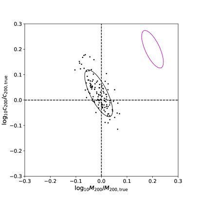
Figure 1: Best-fitting halo mass ($x$-axis) and concentration ($y$-axis) in units of their true values, for 120 Monte-Carlo realisations of ideal haloes generated with a spherical NFW potential. Each dot represents the fit to one halo. Horizontal and vertical black dashed lines mark the equality between best-fitting and true parameters. The black ellipse marks the 1-$\sigma$ scatter of all the measurements. The magenta ellipse in the top right corner shows the average 1-$\sigma$ statistical error for a single halo.

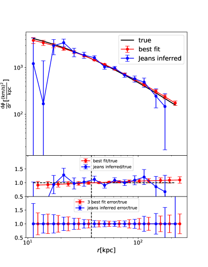
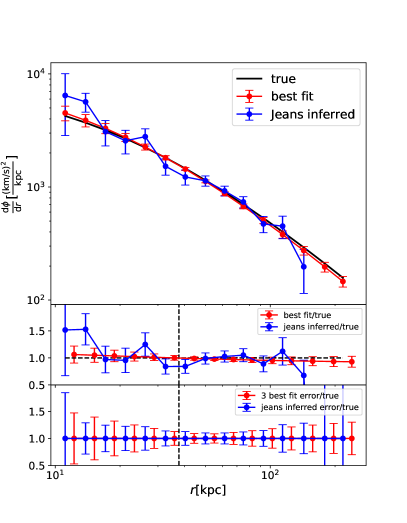
Figure 2: Upper panels show comparisons of true halo potential gradient profiles in the simulation (black), Jeans profiles inferred through Equation 1 (blue) and best-fitting profiles (red) for two randomly selected ideal haloes. Errors on the inferred profile are obtained through 100 bootstrap resamples of the full parent sample, while those on the best-fitting profile are computed from the covariance matrix of the best-fitting parameters. In the middle panel, the Jeans inferred profiles, the best-fitting profiles and the errors are all scaled by the true profile. The bottom panel is similar to the middle panel, except that each is scaled by its own profile to compare only the errors. In this panel, the errors on the best-fitting profiles are increased by a factor of 3, to make an easier comparison with those on the inferred profile. Vertical dashed lines mark the position of the median or half-mass radius for tracers.

Ideal tracers in our analysis are steady state systems generated in a spherical and stationary NFW potential, and thus the SJE should be directly applicable. It is still interesting to apply our method to this system in order to test the performance and understand the error structure in the parameters. The best-fitting halo parameters using Equation 1 are shown in Fig. 1. The statistical error size is comparable to the scatter in the best-fitting parameters (black ellipse in the middle). This is because our ideal tracer sample is free of any systematic uncertainty by construction and the scatter is dominated by statistical errors. We will show in the following sections that using more realistic tracers from cosmological simulations ends up with a much larger difference between statistical errors and the scatter in the best-fitting parameters.

Similar to Wang et al. (2017) and Han et al. (2016b), the statistical error tends to align with a direction of anti-correlation between $M_{200}$ and $c_{200}$. In fact, the anti-correlation between halo mass and concentration (or other combinations of equivalent parameters) is commonly seen in dynamical modelling of the galactic potential (e.g. Deg & Widrow, 2014; Kafle et al., 2014; Wang et al., 2015), despite distinctions among different models. No matter how different the detailed approaches are, they all aim to fit the underlying potential profile, which can be well modelled by a double power law functional form. The parameter anti-correlation may partly arise from such a functional form, as we know power law fitting usually results in anti-correlations between the amplitude parameter and the shape parameter.

The upper panels of Fig 2 show examples of true Jeans inferred and best-fitting potential gradient profiles for two ideal haloes. The differences can be seen more clearly in the middle panels, where we plot profiles normalised by the true one. The errors are scaled by the true profile and are thus relative errors. Over the whole radial range, deviations from the true profile are smaller than the errors, reflecting the fact that for ideal systems the uncertainties are properly modelled by statistical noise.

To clearly show the radial variation of the errors, in the bottom panels we plot the error bars centred at the horizontal unity line. Both reveal a trend of being the smallest in the middle and largest on both smaller and larger scales. The smallest error occurs at a radius which is close but not equal to the median or half-mass radius of tracers (vertical dashed line).

Given the smaller errors on such intermediate scales, the mass inside some intermediate radius can be constrained much better. We have checked that the 1-$\sigma$ uncertainty of the best-fitting mass within the median radius of tracers is smaller than that of $M_{200}$ by a factor of two in log-space. The better constraint of the total mass within the half light radius of tracers in dwarf MW satellite galaxies have been widely reported (e.g. Peñarrubia et al., 2008; Walker et al., 2009; Wolf et al., 2010), though the adopted approaches and discussion are not the same. For example, Wolf et al. (2010) provide the theoretical justification for why the mass within $r_{3}$, the radius where $\mathrm{d}\log\rho_{\ast}/\mathrm{d}\log r=-3$, is insensitive to the velocity anisotropy of tracers. For MW dwarf satellite galaxies, $r_{3}$ is close to the projected half-light radius. In our analysis, $\beta$ at all radii is known directly from the simulation, and the better constrained mass within the median tracer radius is a reflection of the parameter anti-correlation. For parameter combinations along the anti-correlation direction, a larger estimated mass corresponding to a less concentrated profile, while a lower mass corresponding to a more concentrated halo. Thus one would naturally expect the mass profiles predicted by parameter combinations along the anti-correlation direction to cross with each other on some intermediate scale, i.e., the mass within an intermediate scale will have the least uncertainty. Interested readers can find more discussions in Han et al. (2016a).

For Jeans inferred profiles, the smallest error does not have to occur around the median tracer radius, however. This is because for each radial bin, the error size is determined locally and does not depend on the overall radial range of the tracers. The fact that the errors in Fig. 2 are observed to be smallest near the median radius has to be connected to the particular radial distribution of the tracers. The tracers are most sparse on the largest scale, while the phase-space volume is smallest on small scales. This introduces larger variations on those two scales in general. Our current choice of model distribution function and radial ranges happen to lead to a smallest error near the median radius.

5 Tracers in realistic haloes

Ideal tracers demonstrate that when the system is free of systematic sources of bias, our statistical error estimate correctly describes the scatter in best-fitting parameters. In this section we move on to use dark matter particles in MRII and star particles in APOSTLE as our more realistic tracers. We exclude particles in subhaloes and adopt an inner radius cut of 20 kpc for both simulations. The inner cut helps to avoid the central disc region in APOSTLE.

For realistic tracers, there are three sources of systematic errors: (1) Violation of the steady state assumption ($\sigma_{\mathrm{steady}}$) (2) Violation of the spherical assumption ($\sigma_{\mathrm{sph}}$) (3) Violation of the assumed potential profile ($\sigma_{\mathrm{NFW}}$). Accordingly, the covariance matrix of the model parameters can be formally decomposed as a sum of the three plus statistical uncertainty ($\sigma_{\mathrm{stat}}$),

$${\bf C}_{\mathrm{best-fit}}={\bf C}_{\mathrm{steady}}+{\bf C}_{\mathrm{sph}}(+{\bf C}_{\mathrm{NFW}})+{\bf C}_{\mathrm{stat}}.$$ (8)

Wang et al. (2017) showed that results based on true potential templates and the NFW profile give very similar uncertainty in best-fitting parameters if tracers within 20 kpc are excluded. Therefore the effect of (3) is sub-dominant with respect to (1) and (2), and we have put ${\bf C}_{\rm NFW}$ in the bracket. These systematic sources of errors will be investigated in this section. If velocity anisotropy is unknown in the data, additional systematics may be introduced due to improper modelling of this component, and we postpone this discussion to section 6.1.

5.1 Dark matter particles in MRII

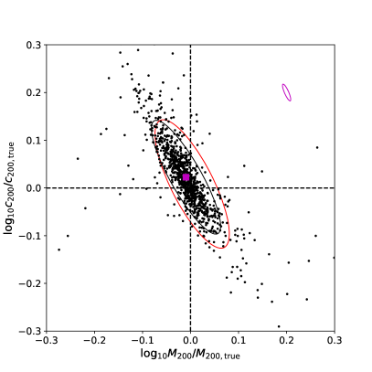
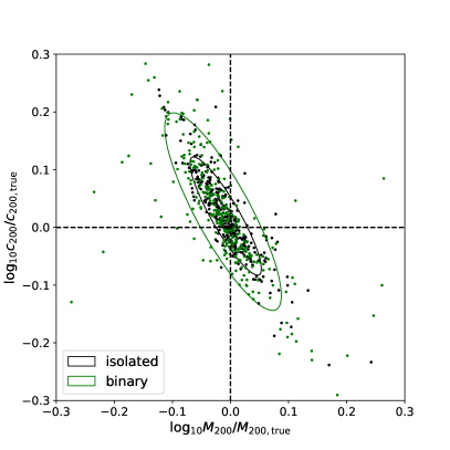
Figure 3: Left: Similar to Fig. 1, but based on all selected haloes in MRII. The black ellipse in the middle and the magenta ellipse in the top right show the average size of the uncertainty in the best-fitting parameters and the statistical errors. The red ellipse in the middle is a reproduction of the uncertainty in the best-fitting parameters in Fig. 1 of Wang et al. (2017) using the oPDF method. Right: Best fits to binary (black) and isolated (green) haloes in MRII. Isolated haloes have been matched in mass to binary haloes to ensure the same halo mass distribution.

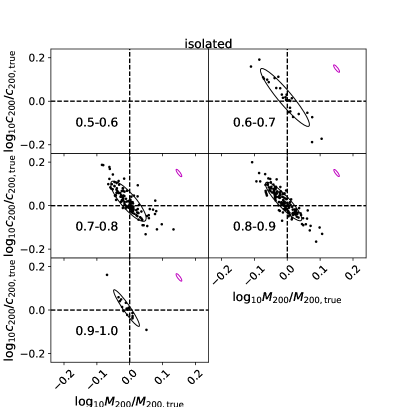
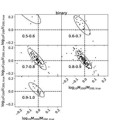
Figure 4: Best-fitting concentration and halo mass for isolated (left) and binary (right) haloes in MRII, shown in separate panels according to the minor-to-major axis ratios of their inertia tensor within $R_{200}$, as labelled on each panel. The small magenta ellipse in each panel of the left plot shows the size of the statistical errors.

Results based on Equation 1 are shown in Fig. 3. The left plot is for all selected isolated and binary haloes as a whole. Similar to Wang et al. (2017), the 1-$\sigma$ uncertainty in best fits (black ellipse) is calculated and plotted by excluding the most biased measurements using 3-$\sigma$ clipping, that is, to first calculate the 1-$\sigma$ uncertainty using all measurements that have converged and then estimate the uncertainty again by excluding data points outside 3 times the size of the 1-$\sigma$ uncertainty. The result indicates a scatter of about 25% in $M_{200}$ and 40% in $c_{200}$.

The uncertainty is close to that of oPDF in Wang et al. (2017) (see the red ellipse in the middle). Although the detailed approaches of oPDF and the SJE are different, they are both based on the steady state and spherical assumptions, and thus we should expect comparable level of uncertainties. According to the Cramer-Rao theorem, maximum likelihood estimators constructed from the full distribution function should be the most efficient. As a result, we would naively expect the oPDF maximum likelihood estimator to give a smaller uncertainty than the SJE, which is based on the momentum of the distribution function. The oPDF predicts the radial distribution of tracers given a model potential and the current radius, radial and tangential velocities of tracers. However, as currently implemented, it obtains the best-fitting halo potential by comparing only the predicted and “observed” radial distributions of the tracers, and thus not all the available information is used, which might explain why the oPDF gives slightly larger uncertainties.

In contrast with results based on the ideal tracer sample above, the statistical error is much smaller than the uncertainty in best-fitting halo parameters, indicating the existence of various systematics (see equation 8). The oPDF gives the same result. Despite the different sizes, both the statistical error and the uncertainty in best fits tend to align with an anti-correlation direction of $M_{200}$ and $c_{200}$. Wang et al. (2017) attributed this alignment to the existence of the first systematic error, ${\bf C}_{\rm steady}$, which is introduced by phase-correlated structures such as streams.

The orbital phase of a particle is a measure of its location on a given orbit (or more precisely, its travel time on the orbit, see Han et al., 2016a, b; Wang et al., 2017 for a more precise definition), while phase-correlation refers to the clustering of particles along the orbit, forming coherently moving structures such as streams. The time evolution of streams thus makes the phase space distribution function of the system evolve over time, violating the steady state assumption. Thus the error introduced by these structures are classified as ${\bf C}_{\rm steady}$. On the other hand, this violation can be largely accounted for if one properly considers the number of phase-independent particles, which is expected to be smaller than the actual number of tracer particles. In other words, ${\bf C}_{\rm steady}$ can be modelled as a statistical error determined by an effective number of phase independent particles. This explains why the error ellipse of the scatter takes similar shape as the statistical error, while the amplitude is larger. Despite the similar origin, Wang et al. (2017) has shown that this effective number is almost independent of the tracer sample size. Accordingly, ${\bf C}_{\rm steady}$ is a systematic uncertainty determined by the intrinsic property of the system. In Section 5.1.1 and Section 5.1.2 we will make further discussions on this interpretation after disentangling different sources of systematics.

The right plot shows in black and green symbols results based on binary and isolated haloes separately. Note the mass distribution of binary haloes are biased to be smaller than that of isolated haloes according to our selection criterion. In order to ensure the same halo mass distribution we have matched each binary halo to one isolated halo according to their $M_{200}$. This is to avoid the bias caused by possible correlations between halo dynamical properties and $M_{200}$.

The uncertainty in best-fitting parameters for the binary population is slightly larger than that of the isolated population, in good agreement with Wang et al. (2017). The reasons are twofold. First, binary haloes are more aspherical than isolated ones. Moreover, the dynamical status of binary haloes are more disturbed than isolated haloes due to the existence of a nearby massive companion. In the following section, we demonstrate these two effects separately.

5.1.1 Deviations from spherical symmetry vs violations of steady state

In order to separate the effect of deviations from spherical symmetry and violations of the steady state assumption, we divide haloes into different subsamples based on their minor-to-major axis ratio, $c/a$, which is computed from the inertia tensor obtained from the mass distributions within $R_{200}$. Results are shown in Fig. 4 for isolated and binary haloes separately.

There is a clear trend for the uncertainty to increase with decreasing $c/a$. Interestingly, we can see clearly that for the binary population, the measurements are biased more and more towards the upper left region for the most elongated haloes. Note this is not seen in Wang et al. (2017). Though oPDF also involves the spherical assumption, Wang et al. (2017) used the true underlying potential profiles as templates when fitting to isolate possible violations of the NFW model, which helped to reduce this effect. In this paper, we focus on the NFW model, but with the oPDF method, we have repeated the analysis using the NFW model and see a similar bias for those most elongated haloes.

There are no isolated haloes with $c/a<0.6$, indicating the existence of more elongated binary haloes. Moreover, for fixed $c/a$, the scatter for binary haloes is larger than for isolated ones. This suggests the larger scatter in the binary population is not only because binaries are more elongated, but also because the dynamical status of binaries are more disturbed, due to the gravitational influence of their companion haloes.

MW and M31 form a binary system, and it is interesting to see where our MW lies in Fig. 4. Vera-Ciro & Helmi (2013) measured its minor to major axis to be 0.8, which is slightly oblate. It sits in the panel where the uncertainty in best-fitting halo parameters is larger than the most spherical haloes, but the average measurement is close to being ensemble unbiased.

The statistical error is almost independent of the halo shape for isolated haloes. For the most spherical haloes with $c/a>0.9$, since violations of the spherical assumption (${\bf C}_{\rm sph}=0$) and deviations from the NFW profile (${\bf C}_{\mathrm{NFW}}\approx 0$) are negligible, the remaining source of systematic error is violations of the steady state assumption, i.e., ${\bf C}_{\rm best-fit}\approx{\bf C}_{\rm steady}+{\bf C}_{\rm stat}$.

The statistical error of these most spherical haloes is still about 5 times smaller than the uncertainty in best fits. If one properly considers the effective number of phase-independent particles, ${\bf C}_{\rm best-fit}$ is expected to be purely statistical. Since the statistical error scales with sample size $N$ as $\sigma^{2}\propto 1/N$, we can have an estimate of the number of phase-independent particles as

$$N_{\rm eff} =N_{\rm tracer}\frac{\sigma^{2}_{\rm stat}}{\sigma^{2}_{\rm best-fit}}$$ (9)

$$=10^{5}\times\left(\frac{1}{5}\right)^{2}$$

$$=4000.$$

This is in good agreement with the number estimated in Wang et al. (2017).

5.1.2 Reducing phase-correlated dynamical tracers

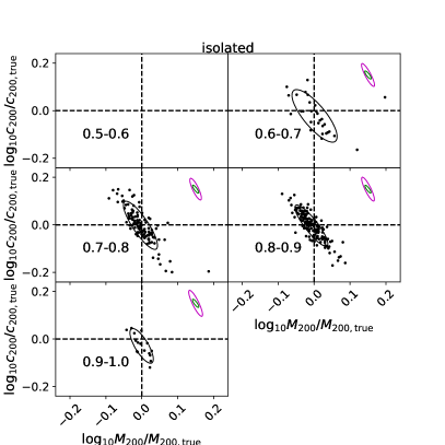
Figure 5: Similar to the left plot of Fig. 4, but each particle has been weighted by the inverse of the total number of particles in the stream to which it belongs. Streams are identified by tracing particles back to their progenitors using the hbt$+$ code of Han et al. (2012, 2017). Magenta ellipses are the new statistical errors after weighting, whereas green ellipses repeat the statistical errors from the left plot of Fig. 4.

The argument of under-estimated statistical errors due to phase-correlated structures can be tested in the following way. The basic idea is to degrade the sample size by down weighting phase-correlated particles. We implement this in an extreme way, by treating particles from the same progenitor as being in a phase-correlated stream, and restricting each stream to contributing only one degree of freedom. After that we can check whether the statistical error is then closer to the uncertainty in best fits, at least for the most spherical haloes.

We start by tracing particles back in time to identify their progenitors, using the halo merger tree built by the hbt$+$ code (Han et al., 2012; Han et al., 2017). hbt$+$ normally does unbinding to remove unbound particles during halo tracking. For the purpose of this study, we have switched off unbinding in hbt$+$ to allow a complete recovery of phase-correlated particles. Particles once belonging to a progenitor at its maximum mass are treated as coming from this progenitor. Note that hierarchical merging of progenitor haloes may lead to the formation of subhalo groups (or groups of streams in our case), which move coherently inside the host halo. Such cases can potentially cause correlations even among different streams, which is hard to account for in our current analysis.

We label the total number of particles in stream i as $N_{i}$, and each particle is assigned a weight of $1/N_{i}$. Smoothly accreted diffuse particles that do not belong to any progenitor haloes are assigned weights of 1. We repeat our analysis in section 3 with this weighted sample. The weights can be thought as the “mass” associated with each particle, which helps to decrease the contribution from massive streams, whose particle number is large but the effective number of phase-uncorrelated particles can be much smaller.

Note, however, this weighting scheme ignores the internal structure of streams. In reality, different streams may contribute different number of phase-independent particles, since the correlation strength among stream particles depends on factors such as the infall time and orbit. Particles in streams accreted earlier have longer time to reach a more phase-mixed status, and hence may contribute a larger number of phase-independent particles. Moreover, with this weighting, the SJE still holds only if all streams are independent populations. This is not necessarily true due to possible correlations among streams mentioned above. So our test is a simplified approach.

Results are presented in Fig. 5. We only show isolated haloes for a clean picture, as for binaries the dynamical status is affected by the massive companion. Compared with the left plot of Fig. 4, the uncertainty in best-fitting halo parameters (${\bf C}_{\mathrm{best-fit}}$) is almost the same, and perhaps only slightly decreased along the major axis of the error ellipse. This suggests that down-weighting stream particles has not led to any significant loss of dynamical information. The statistical errors are inferred from bootstrap sampling as before except that each particle is assigned a weight according to its original stream mass. There is a small change in the shape and direction of the statistical error ellipse, due to the introduction of weights. The error ellipse of best fit parameters also changes correspondingly. Encouragingly, the new statistical errors after weighting are significantly larger and become comparable to the uncertainty in best fits for the most spherical bin. Since ${\bf C}_{\mathrm{best-fit}}={\bf C}_{\mathrm{steady}}+{\bf C}_{\mathrm{stat}}$, this means the systematic caused by phase-correlated particles that violates the steady state assumption, ${\bf C}_{\rm steady}$, is much reduced. This can be understood as contributions from phase-correlated particles are suppressed in bootstrap due to their lower weights, enabling the bootstrap process to correctly sample the variations from phase-independent particles, thus capturing the true degree of freedom of the system.

The test leads support to our argument that phase correlations in streams violate the steady state assumption and cause underestimates of the statistical errors. But we should note various factors that can affect the statistical error size. If the internal structure of streams can be estimated, the statistical error would be smaller. Moreover, correlations between streams mentioned above, if considered, would increase the statistical error. Lastly, smoothly accreted particles might also be phase-correlated due to coherent infall along large cosmic filaments, corresponding to ‘unresolved’ streams. Taking streams which can not be resolved into account, the statistical error size is expected to further increase.

5.2 Stellar tracers in APOSTLE

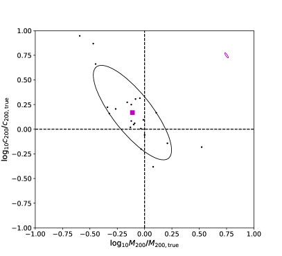
Figure 6: Best-fitting halo parameters for galaxies in the APOSTLE simulations. Points are fits to individual galaxies and the black ellipse marks the 1-$\sigma$ scatter. The magenta solid square is the average parameter of all the galaxies. The tiny magenta ellipse in the top right corner shows the 1-$\sigma$ statistical errors averaged over the entire sample of galaxies. An inner radius cut of 20 kpc has been adopted to exclude the disc component.

The large sample of MRII haloes enables us to compare the systematic uncertainty with statistical noise and investigate the dependence on the halo shape. However, dark matter particle tracers are not representative of real observations. In the following we further test the model performance by using stellar tracers in the APOSTLE simulations, in order to have results more closely related to the real observations.

Results are presented in Fig. 6. Note the axis range is different from that in previous figures. One can see a much larger uncertainty in the best-fitting parameters, which is about a factor of three in both mass and concentration. The statistical error is again much smaller than the uncertainty in best-fitting halo parameters. The true effective number of phase independent particles is estimated to be around only 40. However, due to the small sample size, it is difficult for us to separate contributions from violations of the spherical assumption, and thus this number of 40 should only be regarded as a lower limit.

The larger uncertainty and smaller number of phase independent particles for stars can be understood in the following way. First of all, stars in the stellar halo are usually believed to be stripped from a small number of satellite galaxies, which are hosted by dark matter subhaloes and are the most bound part of those subhaloes. Compared with dark matter particles in these subhaloes, stars are stripped late due to their higher binding energy and thus they have less time to reach a steady state. This introduces stronger violations of the steady state assumption, and it is natural to expect a smaller number of phase independent particles. Moreover, dark matter particles in the host halo are not only formed through stripped particles from substructures, but also through smooth accretion of background particles. These smoothly-accreted particles are expected to be more relaxed and phase independent (Wang et al., 2011). Lastly but importantly, baryonic physics such as mass ejections produced by supernova explosions and stellar winds, can act to violate the steady state assumption of stellar tracers. This process does not exist in dark matter only simulations.

The overall uncertainty in Fig. 6 is in good agreement with Wang et al. (2017), but the measurements are, on average, slightly biased towards the upper left corner. Such an apparent overall bias might be due to the small sample of 24 APOSTLE galaxies. A larger sample might give results that are less ensemble biased. On the other hand, it might indicate some systematics. Wang et al. (2017) have discussed that if using the NFW potential profile to model the underlying potential in hydro-dynamical simulations, the result would be ensemble biased in such a direction. The bias is more obvious with more particles in the inner region included. In fact, Schaye et al. (2015) found that the presence of stars can produce cuspier inner profiles than the NFW model, and the effect is most prominent in haloes of masses about $10^{12}$ to $10^{13}\mathrm{M}_{\odot}$. Since we have excluded particles within 20 kpc, the bias is unlikely to be due to the deviation from the NFW model in inner regions. It is more likely due to the deviation from the spherical assumption (see Fig. 4), as all APOSTLE galaxies are in pairs and the underlying potential profiles are more likely to be more elongated.

6 Discussion

6.1 Constant or improper $\beta$?

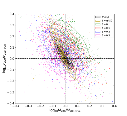
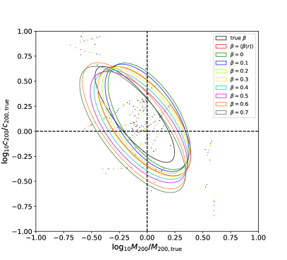
Figure 7: Best-fitting halo parameters when, instead of using the true $\beta(r)$ profiles in the simulation, $\beta$ is assumed to take a fixed values over the whole radial range. Dots and the 1-$\sigma$ uncertainty ellipses are colour coded by the value of $\beta$, indicated in the legend. $\langle\beta(r)\rangle$ is the mean value of $\beta(r)$ averaged over $20~{}{\rm kpc}<r<R_{200}$ and varies for individual haloes. Calculations are shown for MRII (left) and APOSTLE (right). Black dots and ellipses in each panel repeat the results from Fig. 3 and Fig. 6 respectively to enable direct comparisons.

In reality, the tangential velocities of tracers are often missing. As a result, the velocity anisotropy of tracers, $\beta$, cannot be measured directly. To get over this issue, one has to either adopt some fiducial values of $\beta$, or assume a certain parametrised form of $\beta(r)$, and get the best-fitting parameters. In this subsection, we first test the effect of fixing $\beta$ in the left side of Equation 1 to a given value and using the NFW model potential to fit the inferred potential gradient. In the next subsection, we further treat $\beta$ as a free parameter.

Results are presented in Fig. 7, where we fix $\beta$ to a few pre-set values. From $\beta=0$ to larger positive $\beta$, the results gradually change from over-estimated $M_{200}$ ($c_{200}$) to under-estimated $M_{200}$ ($c_{200}$) on average. This can be understood as the degeneracy between $\beta$ and $\mathrm{d}\Phi/\mathrm{d}r$ in Equation 1: to maintain the first term on the left side unchanged, increased $\beta$ corresponds to decreased $\mathrm{d}\Phi/\mathrm{d}r$. The scatter remains almost unchanged with different $\beta$, and is slightly larger for very large (tangential) values of $\beta$ in APOSTLE. This scatter is larger than previous results that used the true $\beta(r)$ profile.

We also test the case when each halo adopts the average $\beta$ of its tracer sample, $\langle\beta(r)\rangle$. The scatter is reduced perpendicular to the mass-concentration anti-correlation direction, because each halo adopts its own average $\beta$ rather than adopting a common pre-set value. However, the scatter along the anti-correlation direction remains larger than the previous result adopting the true $\beta(r)$ profile. Encouragingly, the result becomes mostly ensemble unbiased.

6.2 Radius-independent $\beta$ as a free parameter?

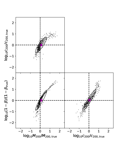
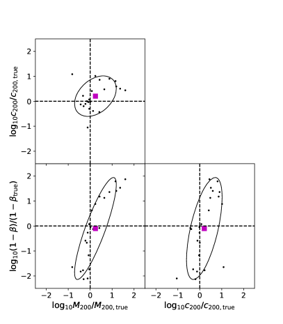
Figure 8: Best-fitting $M_{200}$, $c_{200}$ and $\beta$ for isolated haloes in MRII (left) and galaxies in APOSTLE (right) using Equation 7. The fits are made to the measured radial velocity dispersion profiles of tracers, while $\beta$ is treated as a radius-independent free parameter. The black ellipse and magenta square in each panel mark the 1-$\sigma$ uncertainty and the average measurement.

We now directly fit the measured radial velocity dispersion profiles from the simulations using Equation 7 by treating $\beta$ as a constant but free parameter. This is a common approach adopted in the literature (e.g. Battaglia et al., 2005; Kafle et al., 2014). Note it is different from the approach in Section 6.1, where $\beta$ was fixed to an predefined constant value and the potential gradient inferred from Equation 1 was used for fitting.

Fig. 8 shows results for both isolated MRII haloes and APOSTLE galaxies. Note we focus on isolated haloes in MRII, because the radial density profiles of dark matter tracers are affected by the massive companion halo in binary systems. This makes the integral of Equation 7 hard to converge. The problem does not exist when stars in APOSTLE are used as tracers, because the radial density profiles of stellar tracers drop quickly on large distance.

The axis range is larger than all previous figures. The results end up with much larger uncertainties, which can be as large as one order of magnitude, whereas for APOSTLE galaxies the uncertainty of $\beta$ can be two orders of magnitude. The larger scatter in $\beta$ for APOSTLE is probably because the velocity anisotropy of stars depends more strongly on radius than that of the dark matter, and thus modelling $\beta$ as a free but radius-independent parameter introduces larger systematic errors.

Compared with the large scatter, the measurements averaged over all haloes/galaxies are much closer to zero. There are about 0.1 dex of deviation in the average $M_{200}$ towards the positive direction and in the average $\beta$ towards the negative direction.

$\beta$ shows strong anti-correlations with both $M_{200}$ and $c_{200}$. This trend has already been revealed in Fig. 7 that increased $\beta$ corresponds to underestimated $M_{200}$ and $c_{200}$. Interestingly, marginalising over $\beta$ leaves positive correlation between $M_{200}$ and $c_{200}$, in contrast with the anti-correlation found previously. This means the error is mainly driven by the uncertainty in $\beta$: a large deviation in $\beta$ from the true value leads to large deviations in both $M_{200}$ and $c_{200}$ along the same direction, resulting in the positive correlation between $M_{200}$ and $c_{200}$. This also leads to the comparable size of scatter in the best-fit $M_{200}$ and $c_{200}$ parameters between MRII and APOSTLE. This is in contrast to previous results that APOSTLE galaxies show significantly larger scatters than MRII haloes, when true $\beta$ profiles and Equation 1 are used.

In Fig. 3 and Fig. 4, not only the average statistical error aligns with the uncertainty in best-fits, but also above 98% haloes show an anti-correlation between $M_{200}$ and $c_{200}$ in their individual statistical error. In contrast to Fig. 3, now the statistical errors show significant halo-to-halo scatter and no longer align with the uncertainty in best-fitting halo parameters. Due to the large scatter, it is not straight-forward to compute the average statistical error, which is hence not directly shown in Fig. 3.

We compare measurements within and outside the 1-$\sigma$ uncertainty ellipse in the corresponding parameter plane, and find that for measurements with larger deviations, the radial dependence of $\beta$ is stronger. On average, the $\beta$ profile for measurements outside the 1-$\sigma$ uncertainty ellipse drops faster at $r>100$ kpc by about 30%. However, the halo to halo scatter of the $\beta$ profile is very large, and thus we avoid over-interpreting the result.

6.3 Radial range of tracers

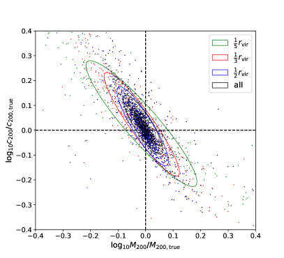
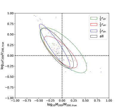
Figure 9: Best-fitting $M_{200}$ and $c_{200}$ when using tracers within a fixed outer radius cut. Each dot represents one halo/galaxy. Measurements are colour coded by the choice of this outer radius, indicated in the legend. Calculations are shown for MRII (left) and APOSTLE (right).

We are interested in the question of what will happen if only tracers within a limited radial range are used. This has been briefly discussed in Wang et al. (2015), where it was found that the total mass within the half-mass radius of all tracers over the whole radial range can be well constrained even when only a subsample of tracers within 60 kpc are used. However, with just five haloes, it is not very clear to see how $M_{200}$ is affected. Here we investigate this using both MRII and APOSTLE haloes and adopt three different radial cuts of $r<\frac{1}{5}R_{200}$, $r<\frac{1}{3}R_{200}$ and $r<\frac{1}{2}R_{200}$. We stick to Equation 1 instead of Equation 7, in order to separate uncertainties due to improper modelling of $\beta$.

Results are presented in Fig. 9. It is clear that with the reduction in tracer outer radius, the measurements show larger and larger overall scatter. The trend is not monotonic for APOSTLE, which might be due to the small sample size. Interestingly, although the scatter is significantly increased for $r<R_{200}/5$, the measurements are still close to be ensemble unbiased, indicating the SJE and the NFW model profiles give good extrapolations to larger radii.

7 Conclusions

The spherical Jeans equation (SJE) has been widely used to probe the mass profile or circular velocity curve of our MW galaxy. In this study we apply the SJE to more than 1000 dark matter haloes in the Millennium-II simulation and 24 MW-like galaxies in the APOSTLE simulations to investigate the performance of the SJE in recovering the halo potential, which we model as an NFW profile.

The large sample of haloes and galaxies enables us to test the model in a statistically robust way. The best-fitting halo mass, $M_{200}$, and concentration, $c_{200}$, suffer from about 25% and 40% systematic uncertainties when dark matter particles in MRII are used as dynamical tracers. When star particles in APOSTLE are used as tracers, the uncertainty can be as large as a factor of three. These uncertainties warn us that inferences based on a single case, such as our MW, are dangerous to make without quoting the large systematic errors behind. The uncertainties are in good agreement with the results of Wang et al. (2017). Although the detailed modelling approach of the oPDF used by Wang et al. (2017) is different from SJE, both the oPDF and SJE assume only steady state tracers and spherical potentials, and thus it is encouraging to see such a good agreement. The systematic uncertainty is attributed to violations of both the steady state and spherical symmetry assumptions. Any dynamical model relying on the two assumptions will suffer from a similar level of uncertainty.

Haloes with minor to major axis ratio less than 0.7 have larger uncertainties and are, on average, biased towards underestimates in $M_{200}$ and overestimates in $c_{200}$. The latter is due to deviations from the NFW model, which can be eliminated if the exact density profiles are used as templates for the fitting (Wang et al., 2017). Binary haloes on average are more elongated and more disturbed than isolated haloes and show larger uncertainties in the fitting.

We further verify the conclusion of Wang et al. (2017) that the statistical errors are underestimated because of phase-correlated structures such as streams. Assuming the statistical errors and the uncertainty in the best-fitting halo parameters would have the same size if one properly considered the true number of phase independent particles for the most spherical haloes , the effective number of phase independent tracer particles is estimated to be about 4000 for dark matter (20 kpc inner cut). For stars, the lower limit is about 40. Such systematic uncertainties cannot be trivially reduced by simply increasing the total sample size, since they are determined by the intrinsic effective number of phase independent particles rather than the total number of particles. We can call this the limiting precision of dynamical modelling of the MW stellar halo.

There are ways to decrease the number of phase-correlated particles. If one can exclude tracers from the few most massive and prominent streams, the phase-correlations would be reduced. In our analysis, we weight particles from the same stream by the inverse of the total particle number in this stream. This helps to down-weight the contribution from massive streams and brings closer agreement in the size of statistical errors and uncertainties in best-fitting halo parameters.

Finally, we investigate the effect of improper modelling with a radius-independent $\beta$ parameter and the effect of only using tracers within a given radial range. Treating $\beta$ as a radius-independent but free parameter, we end up with much larger uncertainties in best-fitting halo mass, concentration and $\beta$ itself. The uncertainty can be as large as one order of magnitude but the average measurements are approximately ensemble-unbiased compared with the large scatter. Under-estimating $\beta$ causes overestimates in $M_{200}$ and $c_{200}$ and vice versa. When $\beta$ is a free parameter, $M_{200}$ positively correlates with $c_{200}$, as the uncertainty becomes primarily driven by the error in $\beta$. Using tracer particles within a given outer radius can significantly increase the uncertainty. Nevertheless, even when only tracers within $R_{200}/5$ are used, the best-fitting halo parameters are almost ensemble unbiased, indicating the SJE and the NFW model profiles give good extrapolations to the outer radius of the dynamical system.

References

- Ablimit & Zhao (2017) Ablimit I., Zhao G., 2017, preprint, (arXiv:1708.00170)
- Battaglia et al. (2005) Battaglia G., et al., 2005, MNRAS, 364, 433
- Boylan-Kolchin et al. (2009) Boylan-Kolchin M., Springel V., White S. D. M., Jenkins A., Lemson G., 2009, MNRAS, 398, 1150
- Boylan-Kolchin et al. (2011) Boylan-Kolchin M., Bullock J. S., Kaplinghat M., 2011, MNRAS, 415, L40
- Cautun et al. (2014) Cautun M., Hellwing W. A., van de Weygaert R., Frenk C. S., Jones B. J. T., Sawala T., 2014, MNRAS, 445, 1820
- Cooper et al. (2010) Cooper A. P., et al., 2010, MNRAS, 406, 744
- Crain et al. (2015) Crain R. A., et al., 2015, MNRAS, 450, 1937
- Deason et al. (2012) Deason A. J., Belokurov V., Evans N. W., An J., 2012, MNRAS, 424, L44
- Deg & Widrow (2014) Deg N., Widrow L., 2014, MNRAS, 439, 2678
- Eadie et al. (2015) Eadie G. M., Harris W. E., Widrow L. M., 2015, ApJ, 806, 54
- Fattahi et al. (2016) Fattahi A., et al., 2016, MNRAS, 457, 844
- Ferrero et al. (2012) Ferrero I., Abadi M. G., Navarro J. F., Sales L. V., Gurovich S., 2012, MNRAS, 425, 2817
- Gnedin et al. (2010) Gnedin O. Y., Brown W. R., Geller M. J., Kenyon S. J., 2010, ApJ, 720, L108
- Han et al. (2012) Han J., Jing Y. P., Wang H., Wang W., 2012, MNRAS, 427, 2437
- Han et al. (2016a) Han J., Wang W., Cole S., Frenk C. S., 2016a, preprint, (arXiv:1507.00769)
- Han et al. (2016b) Han J., Wang W., Cole S., Frenk C. S., 2016b, preprint, (arXiv:1507.00771)
- Han et al. (2017) Han J., Cole S., Frenk C. S., Benitez-Llambay A., Helly J., 2017, preprint, (arXiv:1708.03646)
- Huang et al. (2016) Huang Y., et al., 2016, MNRAS, 463, 2623
- James & Roos (1975) James F., Roos M., 1975, Computer Physics Communications, 10, 343
- Kafle et al. (2012) Kafle P. R., Sharma S., Lewis G. F., Bland-Hawthorn J., 2012, ApJ, 761, 98
- Kafle et al. (2014) Kafle P. R., Sharma S., Lewis G. F., Bland-Hawthorn J., 2014, ApJ, 794, 59
- Kafle et al. (2018) Kafle P. R., Sharma S., Robotham A. S. G., Elahi P. J., Driver S. P., 2018, MNRAS, 475, 4434
- Komatsu et al. (2011) Komatsu E., et al., 2011, ApJS, 192, 18
- Li et al. (2017) Li Z.-Z., Jing Y. P., Qian Y.-Z., Yuan Z., Zhao D.-H., 2017, ApJ, 850, 116
- Lowing et al. (2015) Lowing B., Wang W., Cooper A., Kennedy R., Helly J., Cole S., Frenk C., 2015, MNRAS, 446, 2274
- McMillan (2017) McMillan P. J., 2017, MNRAS, 465, 76
- Navarro et al. (1996) Navarro J. F., Frenk C. S., White S. D. M., 1996, ApJ, 462, 563
- Navarro et al. (1997) Navarro J. F., Frenk C. S., White S. D. M., 1997, ApJ, 490, 493
- Patel et al. (2017) Patel E., Besla G., Mandel K., 2017, MNRAS, 468, 3428
- Peñarrubia et al. (2008) Peñarrubia J., McConnachie A. W., Navarro J. F., 2008, ApJ, 672, 904
- Rossi et al. (2017) Rossi E. M., Marchetti T., Cacciato M., Kuiack M., Sari R., 2017, MNRAS, 467, 1844
- Sakamoto et al. (2003) Sakamoto T., Chiba M., Beers T. C., 2003, A&A, 397, 899
- Sawala et al. (2016) Sawala T., et al., 2016, MNRAS, 457, 1931
- Schaye et al. (2015) Schaye J., Crain R. A., Bower R. G., Furlong M., Schaller M., Theuns T., Dalla Vecchia C., Frenk C. S. e. a., 2015, MNRAS, 446, 521
- Spergel et al. (2003) Spergel D. N., et al., 2003, ApJS, 148, 175
- Vera-Ciro & Helmi (2013) Vera-Ciro C., Helmi A., 2013, ApJ, 773, L4
- Walker et al. (2009) Walker M. G., Mateo M., Olszewski E. W., Peñarrubia J., Wyn Evans N., Gilmore G., 2009, ApJ, 704, 1274
- Wang et al. (2011) Wang J., et al., 2011, MNRAS, 413, 1373
- Wang et al. (2012) Wang J., Frenk C. S., Navarro J. F., Gao L., Sawala T., 2012, MNRAS, 424, 2715
- Wang et al. (2015) Wang W., Han J., Cooper A. P., Cole S., Frenk C., Lowing B., 2015, MNRAS, 453, 377
- Wang et al. (2017) Wang W., Han J., Cole S., Frenk C., Sawala T., 2017, MNRAS, 470, 2351
- Watkins et al. (2010) Watkins L. L., Evans N. W., An J. H., 2010, MNRAS, 406, 264
- Wilkinson & Evans (1999) Wilkinson M. I., Evans N. W., 1999, MNRAS, 310, 645
- Wojtak & Łokas (2010) Wojtak R., Łokas E. L., 2010, MNRAS, 408, 2442
- Wojtak et al. (2008) Wojtak R., Łokas E. L., Mamon G. A., Gottlöber S., Klypin A., Hoffman Y., 2008, MNRAS, 388, 815
- Wojtak et al. (2009) Wojtak R., Łokas E. L., Mamon G. A., Gottlöber S., 2009, MNRAS, 399, 812
- Wolf et al. (2010) Wolf J., Martinez G. D., Bullock J. S., Kaplinghat M., Geha M., Muñoz R. R., Simon J. D., Avedo F. F., 2010, MNRAS, 406, 1220
- Xue et al. (2008) Xue X. X., et al., 2008, ApJ, 684, 1143