A gradient system with a wiggly energy
and relaxed EDP-convergence

1 Introduction

This paper is devoted to the general question of convergence of a family of gradient systems $({\bm{Q}},{\mathcal{E}}_{\varepsilon},{\mathcal{R}}_{\varepsilon})$ towards an effective gradient system $({\bm{Q}},{\mathcal{E}}_{0},{\mathcal{R}}_{\mathrm{eff}})$ when the small parameter $\varepsilon\to 0$. Here ${\bm{Q}}$ is the state space (e.g. a convex subset of a Banach space), ${\mathcal{E}}_{\varepsilon}:[0,T]\times{\bm{Q}}\to{\mathbb{R}}$ are the possibly time-dependent energy functionals, and ${\mathcal{R}}_{\varepsilon}$ are the dissipation potentials such that the gradient-flow equation reads

$$0={\mathrm{D}}_{\dot{q}}{\mathcal{R}}_{\varepsilon}(q_{\varepsilon},\dot{q}_{\varepsilon})+{\mathrm{D}}_{q}{\mathcal{E}}_{\varepsilon}(t,q_{\varepsilon}).$$

The objective is to show that limits $q_{0}$ of solutions $q_{\varepsilon}$ are solutions of the limiting gradient system $({\bm{Q}},{\mathcal{E}}_{0},{\mathcal{R}}_{\mathrm{eff}})$, where typically ${\mathcal{E}}_{0}$ is the -limit of the energies ${\mathcal{E}}_{\varepsilon}$, but in some interesting cases the effective dissipation potential ${\mathcal{R}}_{\mathrm{eff}}$ in the limiting equation

$$0={\mathrm{D}}_{\dot{q}}{\mathcal{R}}_{\mathrm{eff}}(q_{0},\dot{q}_{0})+{\mathrm{D}}_{q}{\mathcal{E}}_{0}(t,q_{0})$$ (1.1)

differs from the -limit ${\mathcal{R}}_{0}$ of the dissipation potentials ${\mathcal{R}}_{\varepsilon}$. However, we are not so much interested in the effective equation, but in the limiting gradient structure $({\bm{Q}},{\mathcal{E}}_{0},{\mathcal{R}}_{\mathrm{eff}})$ that contains additional information to the limiting equation (1.1). Indeed, in (2.1) we give four different gradient structures for the simple ODE $\dot{q}=1-q$.

A general study of -convergence for gradient systems was initiated in [SaS04], which lead to a rich body of research, see [Ste08, Ser11, Bra13, Vis13, Mie16] and the references therein. Several convergence notions are covered by the general name evolutionary -convergence, which emphasizes that evolutionary problems are treated by variational methods involving -convergence for the associated functionals. In this work, we want to generalize the notion of evolutionary -convergence in the sense of the energy-dissipation principle (in short EDP-convergence) introduced in [LM^∗17], which is the first notion that provides a method to calculate the effective dissipation potential ${\mathcal{R}}_{\mathrm{eff}}$ in a unique way.

Our new notion of relaxed EDP-convergence for gradient systems is explained by studying in detail the following wiggly-energy model

$$\nu\dot{u}=-{\mathrm{D}}{\mathcal{E}}_{\varepsilon}(t,u),\quad u(0)=u^{0}\in{\mathbb{R}},$$ (1.2)

with the energy

$${\mathcal{E}}_{\varepsilon}(t,u)=\Phi(u)-\ell(t)u+\varepsilon\kappa(u,\tfrac{\displaystyle 1}{\displaystyle\varepsilon}u),$$

where $\kappa(u,\cdot)$ is a 1-periodic function, and the dissipation potential is simply ${\mathcal{R}}(\dot{u})=\frac{\nu}{2}\dot{u}{}^{2}$. This model was introduced in [Jam96, ACJ96] as a very simple model for explaining slip-stick motions in martensitic phase transformations by starting from a linear viscosity law as in (1.2). See also [Men02, Sul09] for vector-valued versions (i.e. $u(t)\in{\mathbb{R}}^{n}$) of such gradient systems. Earlier models for explaining dry friction go back to Prandtl [Pra28] and Tomlinson [Tom29], see also [PoG12] for historical remarks. The general feature of such models is that a viscous evolution law in a temporally constant, but spatially rapidly varying energetic environment may lead to stick-slip motion, where the limit evolution cannot be a described by the homogenized energy alone. In particular, we find that the effective dissipation potential ${\mathcal{R}}_{\mathrm{eff}}$ is much bigger than ${\mathcal{R}}_{0}={\mathcal{R}}$, where the difference depends on the wiggly part $\kappa$ of the the energy landscape.

Further applications of such models occur in the evolution of phase boundaries in a heterogeneous environment is modeled in [Bha99], based on [AbK88], or in the evolution of dislocations in a slip plane with heterogeneities like forest dislocations [GaM05, GaM06, MoP12, DKW17] (when neglecting lattice friction). Applications to crawling are studied in [GiD17], and an extension to creep is given in [SK^∗09].

A different approach to modeling phase transforming materials by considering connected bistable springs also leads to a complex energy landscape and an evolution in effective wiggly potential [PuT02a, PuT05]. A rigorous derivation of rate-independent one-dimensional pseudo-elasticity is given in [MiT12]. The latter papers as well as [PuT02b, Mie12] are especially devoted to the mathematical justification of the rate-independent case, where $\nu_{\varepsilon}\to 0$ as $\varepsilon\to 0$, such that the limit dynamics doesn’t have any internal time-scale any more.

Here we revisit the general class of scalar wiggly-energy models in the form

$$\partial_{\dot{u}}{\mathcal{R}}(u,\dot{u})=-{\mathrm{D}}_{u}{\mathcal{E}}_{\varepsilon}(t,u),\quad u(0)=u^{0}\in{\mathbb{R}},$$ (1.3)

where ${\mathcal{R}}:{\mathbb{R}}^{2}\to{[0,\infty[}$ is a fixed dissipation potential, i.e. ${\mathcal{R}}(u,0)=0$ and ${\mathcal{R}}(u,\cdot)$ is convex, while the energy ${\mathcal{E}}_{\varepsilon}$ is as above. Thus, (1.3) is the flow induced by the gradient system $({\mathbb{R}},{\mathcal{E}}_{\varepsilon},{\mathcal{R}})$. Under suitable assumptions it is well known from the above works (see e.g. [ACJ96, Men02, PuT02b, Sul09]) that the solutions $u_{\varepsilon}$ of (1.3) converge for $\varepsilon\to 0$ to limits $u_{0}$ that are solutions of the limiting gradient system $({\mathbb{R}},{\mathcal{E}}_{0},{\mathcal{R}}_{\mathrm{eff}})$. We emphasize that ${\mathcal{E}}_{\varepsilon}$ converges uniformly to the limit energy ${\mathcal{E}}_{0}:(t,u)\mapsto\Phi(u)-\ell(t)u$, however, the restoring forces ${\mathrm{D}}{\mathcal{E}}_{\varepsilon}$ do not converge because of the wiggly part involving the non-decaying, oscillatory term $\partial_{y}\kappa(u,\tfrac{\displaystyle 1}{\displaystyle\varepsilon}u)$, where $y$ is used as a placeholder for the second argument $\tfrac{\displaystyle 1}{\displaystyle\varepsilon}u\in{\mathbb{S}}^{1}:={\mathbb{R}}/_{{\mathbb{Z}}}$ of $\kappa$. The major task is then to find the effective dissipation potential ${\mathcal{R}}_{\mathrm{eff}}$, which, as we will see, is larger than ${\mathcal{R}}$ and depends on $\partial_{y}\kappa$.

The purpose of this work is to show how the gradient structure of the underlying problem can be exploited in a natural way using the method for evolutionary -convergence for gradient systems. Thus, we (i) obtain the effective dissipation potential ${\mathcal{R}}_{\mathrm{eff}}$ (and as a by-product the limit evolution) by purely energetic principles, (ii) identify a new mechanical function $(\dot{u},\xi)\mapsto{\mathcal{M}}(u,\dot{u},\xi)$, which we call contact potential, that encodes the effective dissipation law, but which is not a dual pairing in the form ${\mathcal{R}}_{\mathrm{eff}}(u,\dot{u}){+}{\mathcal{R}}^{*}_{\mathrm{eff}}(u,\xi)$, and finally (iii) discuss the convexity properties of ${\mathcal{M}}(u,\cdot,\cdot)$ in the sense of bipotentials, see [BdV08a, BdV08b].

To be more specific, we use the formulation of gradient flows via the following energy-dissipation principle, which originates in the work of De Giorgi [DMT80] and states that (1.3) is equivalent to the energy dissipation balance (EDB) stated below. The EDB asks simply that the final energy plus the dissipated energy equals the initial energy plus the work of the external forces, where the dissipated energy has to be expressed in a particular way in terms of ${\mathcal{R}}$ and its Legendre-Fenchel dual ${\mathcal{R}}^{*}$, namely

$${\mathcal{E}}_{\varepsilon}(T,u(T))+\mathfrak{D}_{\varepsilon}(u)={\mathcal{E}}_{\varepsilon}(0,u(0))+\int_{0}^{T}\partial_{t}{\mathcal{E}}_{\varepsilon}(t,u(t))\;\!\mathrm{d}t,$$ (1.4)

where the dissipation functional $\mathfrak{D}_{\varepsilon}$ is given by

$$\mathfrak{D}_{\varepsilon}(u)=\int_{0}^{T}\!\!\Big{(}{\mathcal{R}}(u(t),\dot{u}(t))+{\mathcal{R}}^{*}\big{(}u(t),-{\mathrm{D}}{\mathcal{E}}_{\varepsilon}(t,u(t))\big{)}\Big{)}\;\!\mathrm{d}t.$$ (1.5)

Several notions of evolutionary -convergence rely on passing to the limit $\varepsilon\to 0$ in (1.4) (cf. [Mie16]) and identifying the limits of the four terms accordingly, see Section 2.

In our case the convergence of $u_{\varepsilon}(t)\to u(t)$ immediately implies, for all $t\in[0,T]$, the convergence ${\mathcal{E}}_{\varepsilon}(t,u_{\varepsilon}(t))\to{\mathcal{E}}_{0}(t,u(t))$ as well as $\partial_{t}{\mathcal{E}}_{\varepsilon}(t,u_{\varepsilon}(t))\to\partial_{t}{\mathcal{E}}_{0}(t,u(t))$. Thus, it remains to understand the limit of ${\mathcal{D}}_{\varepsilon}(u_{\varepsilon})$, and the notion of EDP-convergence asks for the identification of the -limit of $\mathfrak{D}_{\varepsilon}$ on a suitable subset of functions $u\in{\mathrm{W}}^{1,p}(0,T)$ with $p\in{]1,\infty[}$. Our main technical results are in Section 3 and imply the desired statement

$$\mathfrak{D}_{\varepsilon}\overset{\Gamma}{\rightharpoonup}\mathfrak{D}_{0}\quad\text{with }\mathfrak{D}_{0}(u)=\int_{0}^{T}{\mathcal{M}}(u,\dot{u},{-}{\mathrm{D}}{\mathcal{E}}_{0}(t,u))\;\!\mathrm{d}t,$$

The novelty of the notion of EDP-convergence is that we study ${\mathcal{D}}_{\varepsilon}$ not only along the exact solutions $u_{\varepsilon}$ of (1.3) (or equivalently (1.4)), but rather along general functions. This reflects the fact that a given evolution equation $\dot{u}=F(t,u)$ may have different gradient structures, and this difference is only seen by looking at fluctuations around the deterministic solutions, cf. [PRV14, MPR14, LM^∗17]. These fluctuations explore $\mathfrak{D}_{\varepsilon}$ also away from the exact solutions of the gradient flow.

Theorem 2.3 provides the explicit form of the effective contact potential ${\mathcal{M}}$, viz.

$${\mathcal{M}}(u,v,\xi):=\inf\Big{\{}\>\int_{0}^{1}\!\!\Big{(}{\mathcal{R}}(u,|v|\dot{z}(s))+{\mathcal{R}}^{*}\big{(}u,\xi-\partial_{y}\kappa(u,z(s))\big{)}\!\Big{)}{\mathrm{d}}s\;\Big{|}\;z\in{\mathrm{W}}_{v}^{p}(0,1)\>\Big{\}},$$ (1.6)

where ${\mathrm{W}}^{1,p}_{v}:=\{\,z\in{\mathrm{W}}^{1,p}(0,1)\>|\>z(1)-z(0)=\mathop{\mathrm{sign}}(v)\,\}$. The proof is a generalization of the homogenization results in [Bra02] for functionals of the form $u\mapsto\int_{0}^{T}f(t,u,\tfrac{\displaystyle 1}{\displaystyle\varepsilon}u)\;\!\mathrm{d}t$:

In Section 4 we discuss the basic properties of ${\mathcal{M}}$, which allows us to recover the limiting evolution and to identify the effective dissipation potential ${\mathcal{R}}_{\mathrm{eff}}$. In fact, we show

(i) $${\mathcal{M}}(u,v,\xi)\geq\xi v,$$

(ii) $${\mathcal{M}}(u,v,\xi)=\xi v\ \Longleftrightarrow\xi\in\partial_{v}{\mathcal{R}}_{\mathrm{eff}}(u,v)$$

for a unique effective dissipation potential ${\mathcal{R}}_{\mathrm{eff}}$. Thus, all ingredients of relaxed EDP-convergence (cf. Definition 2.2) are established. The main observation here is that the contact sets

$$\mathsf{C}_{{\mathcal{M}}}(u):=\big{\{}\,(v,\xi)\in{\mathbb{R}}^{2}\>\big{|}\>{\mathcal{M}}(u,v,\xi)=\xi v\,\big{\}}$$

can be identified directly giving a general formula for ${\mathcal{R}}_{\mathrm{eff}}$ in terms of a harmonic mean of $y\mapsto\partial_{\xi}{\mathcal{R}}^{*}(u,\xi{-}\partial_{y}\kappa(u,y))$, see Lemma 4.1. Of course, we recover the classical result of [Jam96, ACJ96] for the case ${\mathcal{R}}(u,v)=\frac{1}{2\mu}v^{2}$ and $\kappa(u,y)=\hat{a}\sin(2\pi y)/(2\pi)$, namely

$${\mathcal{R}}_{\mathrm{eff}}(v)=\int_{0}^{|v|}\big{(}\hat{a}^{2}{+}\frac{\hat{v}^{2}}{\mu^{2}}\big{)}^{1/2}{\mathrm{d}}\hat{v}\ \Longleftrightarrow\ \partial{\mathcal{R}}^{*}_{\mathrm{eff}}(\xi)=\mu\,\mathop{\mathrm{sign}}(\xi)\big{(}\max\{\xi^{2}{-}\hat{a}^{2},0\}\big{)}^{1/2}.$$ (1.7)

See also Figure 1.1 for ${\mathcal{R}}_{\mathrm{eff}}$ and the kinetic relation $v=\partial{\mathcal{R}}^{*}_{\mathrm{eff}}(\xi)$. We note that for a non-degenerate wiggly potential this leads to a motion of the interface that is large compared to the excess driving force $\xi-\hat{a}$ near the depinning transition. This is in agreement with experiments, where it is seen that a phase boundary propagates nearly freely when subjected to a driving force above the critical value [EsC93, AbK97].

Figure 1.1: The dissipation potential ${\mathcal{R}}_{\mathrm{eff}}$ and the kinetic relation $v=\partial{\mathcal{R}}^{*}_{\mathrm{eff}}(\xi)$ for the quadratic case, see (1.7).

Hence, $\mathsf{C}_{\mathcal{M}}(u)$ is the graph of a subdifferential of ${\mathcal{R}}_{\mathrm{eff}}(u,\cdot)$ which determines ${\mathcal{R}}_{\mathrm{eff}}$ uniquely, which in the sense of [Vis13] can be understood as ${\mathcal{M}}(u,\cdot,\cdot)$ representing the monotone operator $v\mapsto\partial_{v}{\mathcal{R}}_{\mathrm{eff}}(u,\cdot)$. However, there the function ${\mathcal{M}}(u,\cdot,\cdot)$ is assumed to be convex, which is not the case in our model.

Of course, ${\mathcal{M}}$ contains more information than ${\mathcal{R}}_{\mathrm{eff}}$, and it is worth to study ${\mathcal{M}}$ as such, as we expect it to be relevant as rate function for suitable large deviation limits in the sense of [BoP16]. In Section 4.5 we discuss the question whether ${\mathcal{M}}$ is a bipotential in the sense of [BdV08a, BdV08b], which means that

(i) $${\mathcal{M}}(v,\cdot,\xi)\text{ and }{\mathcal{M}}(u,v,\cdot)\text{ are convex},$$ (1.8a)

(ii) $$v\in\partial_{\xi}{\mathcal{M}}(u,v,\xi)\ \Longleftrightarrow\ {\mathcal{M}}(u,v,\xi)=\xi v\ \Longleftrightarrow\ \xi\in\partial_{v}{\mathcal{M}}(u,v,\xi).$$ (1.8b)

While ${\mathcal{M}}(u,\cdot,\xi)$ is always convex, our Example 4.15 shows that in general ${\mathcal{M}}(u,v,\cdot)$ is non-convex. For the special $p$-homogeneous case ${\mathcal{R}}(u,v)=r(u)|v|^{p}$ we are able to show that ${\mathcal{M}}$ is indeed a bipotential, see Theorem 4.14.

In Section 5 we discuss the results and highlight specific properties of this limit procedure and compare it with recent results in [Vis13, Vis15, Vis17a] concerning related evolutionary -convergence results based on an extended version of the Brezis-Ekeland-Nayroles principle, see Section 5.2. We explicitly show that ${\mathcal{M}}(u,v,\xi)\neq{\mathcal{R}}_{\mathrm{eff}}(u,v){+}{\mathcal{R}}_{\mathrm{eff}}^{*}(u,\xi)$, which implies that there is no EDP-convergence in the sense of [LM^∗17].

Moreover, for converging solutions $u_{\varepsilon}(t)\to u_{0}(t)$ of (1.4) we easily obtain $\mathfrak{D}_{\varepsilon}(u_{\varepsilon})\to\mathfrak{D}_{0}(u_{0})$, i.e. solutions are recovery sequences for the dissipation functional. However, if we separate the dissipation into its primal and its dual part, the corresponding convergences

$$\mathfrak{D}^{\mathrm{prim}}_{\varepsilon}(u_{\varepsilon}):=\int_{0}^{T}{\mathcal{R}}(u_{\varepsilon},\dot{u}_{\varepsilon})\;\!\mathrm{d}t \to\ \mathfrak{D}^{\mathrm{prim}}_{\mathrm{eff}}(u_{0}):=\int_{0}^{T}{\mathcal{R}}_{\mathrm{eff}}(u_{0},\dot{u}_{0})\;\!\mathrm{d}t\quad\text{and}$$

$$\mathfrak{D}^{\mathrm{dual}}_{\varepsilon}(u_{\varepsilon}):=\int_{0}^{T}{\mathcal{R}}^{*}(u_{\varepsilon},{-}{\mathrm{D}}{\mathcal{E}}_{\varepsilon}(t,u_{\varepsilon}))\;\!\mathrm{d}t \to\ \mathfrak{D}^{\mathrm{dual}}_{\mathrm{eff}}(u_{0}):=\int_{0}^{T}{\mathcal{R}}^{*}_{\mathrm{eff}}(u,{-}{\mathrm{D}}{\mathcal{E}}_{0}(t,u))\;\!\mathrm{d}t$$

do not hold. Indeed, for quadratic ${\mathcal{R}}:v\mapsto\frac{\nu}{2}v^{2}$ we always have

$$\mathfrak{D}^{\mathrm{prim}}_{\varepsilon}(u_{\varepsilon})=\mathfrak{D}^{\mathrm{dual}}_{\varepsilon}(u_{\varepsilon})=\frac{1}{2}\mathfrak{D}_{\varepsilon}(u_{\varepsilon})\ \to\ \frac{1}{2}\mathfrak{D}_{0}(u_{0}),$$

but ${\mathcal{R}}_{\mathrm{eff}}$ is such that $\mathfrak{D}^{\mathrm{prim}}_{\mathrm{eff}}(u_{0})\gneqq\mathfrak{D}^{\mathrm{dual}}_{\mathrm{eff}}(u_{0})$ if $\dot{u}_{0}\not\equiv 0$. This shows that the classical approach of [SaS04] is not applicable because of an exchange of dissipation between the dual part $\mathfrak{D}^{\mathrm{dual}}$ and the primal part $\mathfrak{D}^{\mathrm{prim}}$ in the limit $\varepsilon\to 0$. This is again reflected in the fact that ${\mathcal{R}}_{\mathrm{eff}}$ is larger that ${\mathcal{R}}$ and depends on $\partial_{y}\kappa$.

2 Evolutionary -convergence and main results

2.1 The energy-dissipation principle for gradient system

To explain the general structure between our special model of (1.3) we use general ordinary differential equation (ODE) $\dot{q}={\bm{F}}(t,q)\in{\mathbb{R}}^{n}$ and general gradient systems (GS) $({\bm{Q}},{\bm{E}},{\bm{R}})$, where ${\bm{Q}}={\mathbb{R}}^{n}$ is the state space, ${\bm{E}}:[0,T]\times{\bm{Q}}\to{\mathbb{R}}$ is a sufficiently smooth, time-dependent energy functional, and ${\bm{R}}:{\bm{Q}}\times{\bm{Q}}\to{[0,\infty[}$ is a sufficiently smooth dissipation potential. By ${\bm{R}}^{*}$ we denote the (Legendre-Fenchel) dual dissipation potential defined via ${\bm{R}}^{*}(q,{\bm{\xi}})=\sup\{\,\langle{\bm{\xi}},{\bm{v}}\rangle-{\bm{R}}(q,{\bm{v}})\>|\>{\bm{v}}\in{\bm{Q}}\,\}$.

We say that the ODE $\dot{q}={\bm{F}}(t,q)$ has a gradient structure or is a gradient flow if there exists a GS $({\bm{Q}},{\bm{E}},{\bm{R}})$ such that ${\bm{F}}(t,q)=\partial_{\bm{\xi}}{\bm{R}}^{*}(q,{-}{\mathrm{D}}_{q}{\bm{E}}(t,q))$. In that case, we also say that the ODE is a generated by the GS $({\bm{Q}},{\bm{E}},{\bm{R}})$. We emphasize that one ODE can have several distinct gradient structures, e.g. $\dot{q}=1-q\in{\mathbb{R}}$ is generated by the gradient systems $({[0,\infty[},{\bm{E}}_{j},{\bm{R}}_{j})$ for $j=1,\ldots,4$ with with

$${\bm{E}}_{1}(q)={\bm{E}}_{2}(q)=\frac{1}{2}(1{-}q)^{2},\quad{\bm{R}}^{*}_{1}(\xi)=\frac{1}{2}\xi^{2},\quad{\bm{R}}^{*}_{2}(q,\xi)=\frac{\frac{1}{2}\xi^{2}+\frac{1}{4}\xi^{4}}{1+(1{-}q)^{2}},$$ (2.1)

$${\bm{E}}_{3}(q)={\bm{E}}_{4}(q)=q\log q-q+1,\ {\bm{R}}^{*}_{3}(q,\xi)=\frac{q{-}1}{2\log q}\xi^{2},\quad{\bm{R}}_{4}^{*}(q,v)=2\sqrt{q}\,\big{(}\!\cosh(\tfrac{1}{2}\xi)-1\big{)}.$$

We also refer to [PRV14, MPR14] for discussion of different gradient structures for the heat equation or for finite-state Markov processes. Thus, we emphasize that the gradient structure of a given ODE has additional physical information, e.g. about the microscopic origin of the ODE, see [LM^∗17]. This is seen in the above case, since we may choose different energies ${\bm{E}}_{j}$ and even for one chosen ${\bm{E}}_{j}$ we may choose different dissipation functionals ${\bm{R}}_{k}$.

We recall that the evolution law associated with a gradient system can be written in two equivalent ways, namely

$$0\in\partial_{\dot{q}}{\mathcal{R}}(q,\dot{q})+{\mathrm{D}}_{q}{\mathcal{E}}(t,q)\quad\Longleftrightarrow\quad\dot{q}\in\partial_{\xi}{\mathcal{R}}^{*}(q,{-}{\mathrm{D}}_{q}{\mathcal{E}}(t,q)).$$ (2.2)

The energy-dissipation principle states that under reasonable technical assumptions these relations are equivalent to a scalar energy-dissipation balance. To motivate this we consider a lower semi-continuous convex function $\Psi:X\to{\mathbb{R}}_{\infty}$ on a reflexive Banach space $X$. Denote by $\Psi^{*}:X^{*}\to{\mathbb{R}}_{\infty}$ the Legendre-Fenchel dual, i.e. $\Psi(\xi)=\sup\{\,\langle\xi,v\rangle-\Psi(v)\>|\>v\in X\,\}$. Then, the Fenchel equivalences (see [Fen49, EkT76] or [Roc70, Thm 23.5]) state that

$$\text{(i) }\xi\in\partial\Psi(v)\quad\Longleftrightarrow\quad\text{(ii) }v\in\partial\Psi^{*}(\xi)\quad\Longleftrightarrow\quad\text{(iii) }\Psi(v)+\Psi^{*}(\xi)=\langle\xi,v\rangle,$$

where $\partial$ denotes the convex subdifferential. Indeed, by the definition of $\Psi^{*}$ we have the Fenchel-Young inequality $\Psi(v)+\Psi^{*}(\xi)\geq\langle\xi,v\rangle$ for all $v\in X$ and $\xi\in X^{*}$. Thus, in (iii) it would suffices to ask for the inequality $\Psi(v)+\Psi^{*}(\xi)\leq\langle\xi,v\rangle$.

Applying this with $\Psi={\mathcal{R}}(q,\cdot)$, integration over time and using the chain rule we see that $q$ solves (2.2) if and only if $q$ satisfies the energy-dissipation balance

$${\mathcal{E}}(T,q(T))+\mathfrak{D}(q)={\mathcal{E}}(0,q(0))-\int_{0}^{T}{\mathrm{D}}_{t}{\mathcal{E}}(t,q(t))\;\!\mathrm{d}t,$$ (2.3)

$$\text{where }\mathfrak{D}(q):=\int_{0}^{T}\Big{(}{\mathcal{R}}(q,\dot{q})+{\mathcal{R}}^{*}\big{(}q,-{\mathrm{D}}_{q}{\mathcal{E}}(t,q)\big{)}\Big{)}\;\!\mathrm{d}t.$$

Indeed, using the chain rule $\frac{{\mathrm{d}}}{{\mathrm{d}}t}{\mathcal{E}}(t,q(t))={\mathrm{D}}_{t}{\mathcal{E}}(t,q(t))+\langle{\mathrm{D}}_{q}{\mathcal{E}}(t,q(t)),\dot{q}(t)\rangle$ (the validity of which is the main technical assumption in the general infinite-dimensional case) it is easy to go back from (2.3) to (2.2), as we deduce

$$\int_{0}^{T}\Big{(}{\mathcal{R}}(q,\dot{q})+{\mathcal{R}}^{*}\big{(}q,-{\mathrm{D}}_{q}{\mathcal{E}}(t,q)\big{)}-\langle{\mathrm{D}}_{q}{\mathcal{E}}(t,q(t)),\dot{q}(t)\rangle\Big{)}\;\!\mathrm{d}t=0.$$

As the integrand in non-negative by the Fenchel-Young inequality and the integral is $0$, we conclude that the integrand is $0$ almost everywhere, which means (iii) in the Fenchel equivalences. Thus (i) and (ii) also hold almost everywhere, i.e. (2.2) holds. We refer to [AGS05, Mie16] for more details and exact statements.

2.2 Evolutionary -convergence for gradient systems

We now consider families $(Q,{\mathcal{E}}_{\varepsilon},{\mathcal{R}}_{\varepsilon})$ of gradient systems depending on a small parameter $\varepsilon>0$. We are interested in the limits $u_{0}$ of solutions as well as in suitable limiting gradient systems $(Q,{\mathcal{E}}_{0},{\mathcal{R}}_{0})$.

Hence, for $\varepsilon\in[0,\varepsilon_{0}]$ we consider the gradient-flow equations

$$0=\partial_{\dot{u}}{\mathcal{R}}_{\varepsilon}(q_{\varepsilon},\dot{q}_{\varepsilon})+{\mathrm{D}}_{q}{\mathcal{E}}_{\varepsilon}(t,q_{\varepsilon}),\quad q_{\varepsilon}(0)=q^{0}_{\varepsilon}.$$ (2.4)

Following [Mie16] we say that the family $(Q,{\mathcal{E}}_{\varepsilon},{\mathcal{R}}_{\varepsilon})$ of gradient systems E-converges the gradient system $(Q,{\mathcal{E}}_{0},{\mathcal{R}}_{0})$, and shortly write $(Q,{\mathcal{E}}_{\varepsilon},{\mathcal{R}}_{\varepsilon})\overset{{\mathrm{E}}}{\to}(Q,{\mathcal{E}}_{0},{\mathcal{R}}_{0})$, if the following holds: If $q_{\varepsilon}^{0}\to q_{0}^{0}$ and $q_{\varepsilon}:[0,T]\to Q$ are solutions of (2.4) for $\varepsilon\in{]0,\varepsilon_{0}[}$, then there exist a subsequence $0<\varepsilon_{k}\to 0$ and a solution $q_{0}:[0,T]\to Q$ for (2.4) with $\varepsilon=0$ such that

$$\forall\,t\in{]0,T]}:\quad q_{\varepsilon_{k}}(t)\to q_{0}(t)\text{ and }{\mathcal{E}}_{\varepsilon_{k}}(t,q_{\varepsilon_{k}}(t))\to{\mathcal{E}}_{0}(t,q_{0}(t)).$$ (2.5)

(A similar notion $\overset{{\mathrm{E}}}{\rightharpoonup}$ can be defined by replacing strong with weak convergence.) Note that the selection of subsequences is only needed if the limiting underlying gradient systems does not have uniqueness of solutions. In that case different subsequences may converge for to different solutions of (2.4)_ε=0 with the same initial condition $q_{0}^{0}$.

A major drawback of this notion is that ${\mathcal{R}}_{0}$ is not intrinsically connected to the original gradient systems $(Q,{\mathcal{E}}_{\varepsilon},{\mathcal{R}}_{\varepsilon})$. Indeed, if $(Q,{\mathcal{E}}_{0},{\mathcal{R}}_{0})$ and $(Q,{\mathcal{E}}_{0},\widehat{\mathcal{R}}_{0})$ generate the same gradient-flow equation (i.e. $\partial_{\xi}{\mathcal{R}}_{0}^{*}(q,{-}{\mathrm{D}}_{q}{\mathcal{E}}_{0}(t,q))=\partial_{\xi}\widehat{\mathcal{R}}_{0}^{*}(q,{-}{\mathrm{D}}_{q}{\mathcal{E}}_{0}(t,q))$, see (2.1) for examples) and if $(Q,{\mathcal{E}}_{\varepsilon},{\mathcal{R}}_{\varepsilon})\overset{{\mathrm{E}}}{\to}(Q,{\mathcal{E}}_{0},{\mathcal{R}}_{0})$, then we also have $(Q,{\mathcal{E}}_{\varepsilon},{\mathcal{R}}_{\varepsilon})\overset{{\mathrm{E}}}{\to}(Q,{\mathcal{E}}_{0},\widehat{\mathcal{R}}_{0})$. The notion of EDP convergence is stricter and involves the effective dissipation potential ${\mathcal{R}}_{\varepsilon}$ for $\varepsilon\in{[0,\varepsilon_{0}[}$ directly through the dissipation functionals $\mathfrak{D}_{\varepsilon}$ defined via

$$\mathfrak{D}_{\varepsilon}(q(\cdot)):=\int_{0}^{T}\Big{(}{\mathcal{R}}_{\varepsilon}(q,\dot{q})+{\mathcal{R}}_{\varepsilon}^{*}\big{(}q,{-}{\mathrm{D}}_{q}{\mathcal{E}}_{\varepsilon}(t,q)\big{)}\Big{)}\;\!\mathrm{d}t.$$ (2.6)

The following definition now asks -convergence of $\mathfrak{D}_{\varepsilon}$ to $\mathfrak{D}_{0}$, and thus ${\mathcal{R}}_{\varepsilon}$ are intrinsically involved. The new feature is that we ask much more than convergence of these functionals along solutions $q_{\varepsilon}$ converging to $q_{0}$. In light of [LM^∗17] this seems to be essential, since the gradient structures contain more information than the equations determining the solutions. We refer to the discussion in Section 5.

Definition 2.1 (EDP-convergence, cf. [LM^∗17])

 The gradient systems $(Q,{\mathcal{E}}_{\varepsilon},{\mathcal{R}}_{\varepsilon})_{]0,\varepsilon_{0}]}$ are said to converge to the gradient system $(Q,{\mathcal{E}}_{0},{\mathcal{R}}_{0})$ in the sense of the energy-dissipation principle, shortly “EDP-converge” or $(Q,{\mathcal{E}}_{\varepsilon},{\mathcal{R}}_{\varepsilon})_{]0,\varepsilon_{0}[}\overset{\mathrm{EDP}}{\longrightarrow}(Q,{\mathcal{E}}_{0},{\mathcal{R}}_{0})$, if the following conditions hold:

$$(Q,{\mathcal{E}}_{\varepsilon},{\mathcal{R}}_{\varepsilon})\overset{{\mathrm{E}}}{\to}(Q,{\mathcal{E}}_{0},{\mathcal{R}}_{0}),$$ (2.7a)

$${\mathcal{E}}_{\varepsilon}\overset{\Gamma}{\to}{\mathcal{E}}_{0},\quad\text{ and }\quad\mathfrak{D}_{\varepsilon}\overset{\Gamma}{\rightharpoonup}\mathfrak{D}_{0},$$ (2.7b)

where specific choice of the -convergence $\overset{\Gamma}{\rightharpoonup}$ in (2.7b) needs to be specified in each particular case.

Two remarks are in order. First, as we highlight in Section 5, the EDP-convergence does in general not imply that the two contributions of the dissipation function (generated by ${\mathcal{R}}_{\varepsilon}$ and ${\mathcal{R}}_{\varepsilon}^{*}$, respectively) converge individually. Indeed, this may even be wrong when restricting to solutions.

Second, it is one of the main results of this paper that the structure of $\mathfrak{D}_{\varepsilon}$ may not be preserved by taking the -limit in general. Under suitable technical assumptions the techniques in [Dal93] show that a -limit $\mathfrak{D}_{0}$ has the integral form $\mathfrak{D}_{0}(q)=\int_{0}^{T}{\mathcal{N}}_{0}(t,q,\dot{q})\;\!\mathrm{d}t$, but ${\mathcal{N}}_{0}$ may not have the form

$${\mathcal{N}}_{0}(t,q,\dot{q})={\mathcal{R}}_{0}(q,\dot{q})+{\mathcal{R}}^{*}_{0}(q,{-}{\mathrm{D}}_{q}{\mathcal{E}}_{0}(t,q))$$

for any ${\mathcal{R}}_{0}$.

In our wiggly-energy model as well as in many other applications we have a time-dependent external loading $\ell:[0,T]\to Q^{*}$, and we want to have a result that works uniformly in with respect to $\ell$. Thus, we look at driven gradient systems with

$${\mathcal{E}}_{\varepsilon}(t,q)={\mathcal{F}}_{\varepsilon}(q)-\langle\ell(t),q\rangle\quad\text{and}\quad{\mathcal{F}}_{\varepsilon}\overset{\Gamma}{\to}{\mathcal{F}}_{0}.$$

Because of ${\mathrm{D}}_{q}{\mathcal{E}}_{\varepsilon}(t,q)={\mathrm{D}}{\mathcal{F}}_{\varepsilon}(q)-\ell(t)$ and the arbitrariness of $\ell$, we introduce the variable $\xi\in Q^{*}$ as a placeholder of variants for the restoring force $-{\mathrm{D}}_{q}{\mathcal{E}}_{\varepsilon}$. Indeed, we use the decomposition

$$-{\mathrm{D}}_{q}{\mathcal{E}}_{\varepsilon}(t,q)=\Xi_{\varepsilon}(q)+\ell(t)-\Omega_{\varepsilon}(q),$$ (2.8)

where $\Xi_{\varepsilon}$ is supposed to converge nicely to the desired limit ${\mathrm{D}}{\mathcal{F}}_{0}(q)$, while $\Omega_{\varepsilon}(a)$ somehow converges to $0$. Thus, we can write $\mathfrak{D}_{\varepsilon}$ in the form

$$\mathfrak{D}_{\varepsilon}(q)=\mathfrak{J}_{\varepsilon}\big{(}q,-{\mathrm{D}}_{q}{\mathcal{E}}_{\varepsilon}(t,q){+}\Omega_{\varepsilon}(q)\big{)},\quad\text{where }$$

$$\mathfrak{J}_{\varepsilon}(q,\xi)=\int_{0}^{T}\Big{(}{\mathcal{R}}_{\varepsilon}(q,\dot{q})+{\mathcal{R}}_{\varepsilon}^{*}\big{(}q,\xi{-}\Omega_{\varepsilon}(q)\big{)}\Big{)}\;\!\mathrm{d}t.$$ (2.9)

As is observed in [Vis13] it is important that $\dot{q}$ and $\xi$ are in duality and that the convergences of $\dot{q}_{\varepsilon}$ to $\dot{q}_{0}$ and of $\xi_{\varepsilon}$ to $\xi_{0}$ are such that the duality pairing $(\dot{q},\xi)\mapsto\int_{0}^{T}\langle\xi(t),\dot{q}(t)\rangle\;\!\mathrm{d}t$ is continuous. In most applications one uses

$$q_{\varepsilon}\rightharpoonup q_{0}\text{ in }{\mathrm{W}}^{1,p}(0,T;Q)\text{ (weakly)}\quad\text{and}\quad\xi_{\varepsilon}\to\xi_{0}\text{ in }{\mathrm{L}}^{p^{\prime}}(0,T;Q^{*})\text{ (strongly)}.$$ (2.10)

This explains why the decomposition (2.8) is useful: we obtain the strong convergence $\Xi_{\varepsilon}(q_{\varepsilon}(\cdot))\to\Xi_{0}(q_{0}(\cdot))$ and want to use $\Omega_{\varepsilon}(q(\cdot))\rightharpoonup 0$ in a suitable sense.

Now, we may consider -convergence for the functionals $\mathfrak{J}_{\varepsilon}$ with respect to the convergence in (2.10), denoted by “$\xrightarrow[\!\!{}^{{\mathrm{w}}{\times}{\mathrm{s}}}\!\!]{}$”. Again, under suitable assumption the theory in [Dal93] predicts that a possible -limit takes the following form

$$\mathfrak{J}_{\varepsilon}\overset{\Gamma}{\xrightarrow[\!\!{}^{{\mathrm{w}}{\times}{\mathrm{s}}}\!\!]{}}\mathfrak{J}_{0}:(q,\xi)\mapsto\int_{0}^{T}{\mathcal{M}}(q,\dot{q},\xi)\;\!\mathrm{d}t,$$ (2.11)

where now ${\mathcal{M}}(q,\cdot,\cdot):Q\times Q^{*}\to[0,\infty]$ contains the effective information on the dissipation for a given macroscopic speed $v=\dot{q}\in Q$ and an effective macroscopic force $\xi\in Q^{*}$. Even in the case $\Omega_{\varepsilon}\equiv 0$ we see that the convergence $\xrightarrow[\!\!{}^{{\mathrm{w}}{\times}{\mathrm{s}}}\!\!]{}$ from (2.10) is the natural one for studying the -limit of $\mathfrak{J}_{\varepsilon}$, since under suitable coercivity assumptions one has

$${\mathcal{R}}_{\varepsilon}(q,\cdot)\overset{\Gamma}{\rightharpoonup}{\mathcal{R}}_{0}(q,\cdot)\text{ in }Q\quad\Longleftrightarrow\quad{\mathcal{R}}_{\varepsilon}^{*}(q,\cdot)\overset{\Gamma}{\to}{\mathcal{R}}_{0}^{*}(q,\cdot)\text{ in }Q^{*},$$

see [Att84, p. 271] and the survey [Mie16, Sec. 3.2].

As a remainder of the Young-Fenchel inequality ${\mathcal{R}}_{\varepsilon}(q,v)+{\mathcal{R}}_{\varepsilon}^{*}(q,\xi)\geq\langle\xi,v\rangle$ one can hope for the estimate

$$\forall\,q,v\in Q,\ \xi\in Q^{*}:\quad{\mathcal{M}}(q,v,\xi)\geq\langle\xi,v\rangle,$$ (2.12)

however this has to be proved in each case using properties of $\Omega_{\varepsilon}$, see our Lemma 4.1(b) for the wiggly-energy model. Then, the essential as in the energy-dissipation principle of the previous subsection the limit evolution is given by

$${\mathcal{M}}(q,\dot{q},{-}{\mathrm{D}}_{q}{\mathcal{E}}_{0}(t,q))=-\langle{\mathrm{D}}_{q}{\mathcal{E}}_{0}(t,q),\dot{q}\rangle\text{ \ or equivalently}$$

$${\mathcal{E}}_{0}(T,q(t))+\int_{0}^{T}\!\!{\mathcal{M}}(q,\dot{q},{-}{\mathrm{D}}_{q}{\mathcal{E}}_{0}(t,q))\;\!\mathrm{d}t={\mathcal{E}}_{0}(0,q(0))-\int_{0}^{T}\langle\dot{\ell}(t),q\rangle\;\!\mathrm{d}t,$$

where we assumed that ${\mathcal{E}}_{0}(t,q)={\mathcal{F}}_{0}(q)-\langle\ell(t),q\rangle$ still satisfies a chain rule. While ${\mathcal{M}}$ encodes information on the combined limit of $({\mathcal{E}}_{\varepsilon},{\mathcal{R}}_{\varepsilon})$, we can now go back looking at solutions which necessarily stay in the so-called contact set $\mathsf{C}_{{\mathcal{M}}}(\cdot)$, namely

$$(\dot{q}(t),{-}{\mathrm{D}}_{q}{\mathcal{E}}_{0}(t,q(t))\in\mathsf{C}_{{\mathcal{M}}}(q(t))\text{ with }\mathsf{C}_{\mathcal{M}}(q):=\big{\{}\,(v,\xi)\in Q\times Q^{*}\>\big{|}\>{\mathcal{M}}(q,v,\xi)=\langle\xi,v\rangle\,\big{\}}.$$

This subset gives the admissible pairs $(v,\xi)$ of rates and forces at a given state $q$, i.e. it defines a kinetic relation.

Our definition of relaxed EDP-convergence now asks that this kinetic relation is given in terms of a dissipation potential ${\mathcal{R}}_{\mathrm{eff}}$. We emphasize that using this approach the dissipation ${\mathcal{R}}_{\mathrm{eff}}$ is uniquely defined through the steps above, i.e. as in EDP-convergence we find “the” effective dissipation potential, however in contrast to EDP-convergence we are more flexible in term of the -limit $\mathfrak{D}_{0}$ of $\mathfrak{D}_{\varepsilon}$, which may not have $({\mathcal{R}}_{0},{\mathcal{R}}_{0}^{*})$ form. That is also the reason why we use the notation ${\mathcal{R}}_{\mathrm{eff}}$, as there is no direct convergence of ${\mathcal{R}}_{\varepsilon}$ to ${\mathcal{R}}_{\mathrm{eff}}$, see the discussion in Section 5.

Definition 2.2 (Relaxed EDP-convergence)

We say that the family $(Q,{\mathcal{E}}_{\varepsilon},{\mathcal{R}}_{\varepsilon})_{]0,\varepsilon_{0}[}$ of gradient systems converges to the gradient system $(Q,{\mathcal{E}}_{0},{\mathcal{R}}_{\mathrm{eff}})$ in the relaxed EDP sense, and shortly write $(Q,{\mathcal{E}}_{\varepsilon},{\mathcal{R}}_{\varepsilon})_{]0,\varepsilon_{0}[}\xrightarrow{\mathrm{relEDP}}(Q,{\mathcal{E}}_{0},{\mathcal{R}}_{\mathrm{eff}})$, if the following holds.

$$(Q,{\mathcal{E}}_{\varepsilon},{\mathcal{R}}_{\varepsilon})_{]0,\varepsilon_{0}[}\overset{{\mathrm{E}}}{\to}(Q,{\mathcal{E}}_{0},{\mathcal{R}}_{\mathrm{eff}}),$$ (2.13a)

$${\mathcal{E}}_{\varepsilon}(t,q)={\mathcal{F}}_{\varepsilon}(q)-\langle\ell(t),q\rangle,\quad{\mathcal{F}}_{\varepsilon}\overset{\Gamma}{\to}{\mathcal{F}}_{0},$$ (2.13b)

$$\exists\,\Omega_{\varepsilon}:\ \widetilde{q}_{\varepsilon}\rightharpoonup\widetilde{q}_{0}\text{ in }{\mathrm{W}}^{1,p}(0,T;Q)\Longrightarrow{\mathrm{D}}_{q}{\mathcal{F}}_{\varepsilon}(\cdot,\widetilde{q}_{\varepsilon}){-}\Omega_{\varepsilon}(\widetilde{q}_{\varepsilon})\to{\mathrm{D}}_{q}{\mathcal{F}}_{0}(\widetilde{q}_{0}),$$ (2.13c)

$$\mathfrak{J}_{\varepsilon}\text{ defined in \eqref{eq:def.mfJeps} satisfies \eqref{eq:mfJ.cvg} with }{\mathcal{M}}\text{ satisfying \eqref{eq:genYouFen}},$$ (2.13d)

$$\exists\,\text{diss.\,pot.\,}{\mathcal{R}}_{\mathrm{eff}}\ \forall\,q\in Q:\ \mathsf{C}_{{\mathcal{M}}}(q)=\big{\{}\,(v,\xi)\in Q\times Q^{*}\>\big{|}\>\xi\in\partial_{v}{\mathcal{R}}_{\mathrm{eff}}(q,v)\,\big{\}}.$$ (2.13e)

The aim of this paper is to show that the theory sketched above can be made rigorous for the wiggly-energy model. Thus, we have a first non-trivial example that shows that relaxed EDP-convergence provides a mechanically relevant concept for deriving effective gradient structures where neither the Sandier-Serfaty theory [SaS04] nor the EDP-convergence from [LM^∗17] applies.

2.3 Our model as gradient system and relaxed EDP-convergence

For our wiggly-energy model, the gradient system is given by the state space ${\mathbb{R}}$, the energy ${\mathcal{E}}^{\mathrm{wig}}_{\varepsilon}:{\mathbb{R}}\times[0,T]\to{\mathbb{R}}$ and a general convex dissipation potential ${\mathcal{R}}:{\mathbb{R}}\times{\mathbb{R}}\to{\mathbb{R}}$. We choose the following assumptions to keep the technicalities to a limit; however, it is easily possible to generalize most assumptions except for the additive structure of ${\mathcal{E}}_{\varepsilon}$ concerning the wiggly part $\kappa$.

$${\mathcal{E}}^{\mathrm{wig}}_{\varepsilon}(t,u)=\Phi(u)-\ell(t)u+\varepsilon\kappa(u,\tfrac{\displaystyle 1}{\displaystyle\varepsilon}u)\text{ with }\Phi\in{\mathrm{C}}^{1}({\mathbb{R}}),\ \ell\in{\mathrm{C}}^{1}([0,T])$$ (2.14a)

$$\text{ and }\kappa\in{\mathrm{C}}^{1}({\mathbb{R}}^{2})\text{ with }\kappa(u,y{+}1)=\kappa(u,y)\text{ for all }u,y\in{\mathbb{R}};$$ (2.14b)

$${\mathcal{R}}\in{\mathrm{C}}^{1}({\mathbb{R}}^{2}),\quad{\mathcal{R}}(u,v)\geq 0,\quad{\mathcal{R}}(u,0)=0;$$ (2.14c)

$$\forall\,u\in{\mathbb{R}}:\ {\mathcal{R}}(u,\cdot)\text{ is strictly convex};$$ (2.14d)

$$\exists\,p\in{]1,\infty[}\ \exists\,c_{1},c_{2}>0\ \exists\ \text{modulus of continuity }\omega\ \>\forall\,u,\,\widehat{u},\,v\in{\mathbb{R}}:$$

$$\qquad c_{1}(|v|^{p}{-}1)\leq{\mathcal{R}}(u,v)\leq c_{2}(1{+}|v|^{p})\text{ and}$$ (2.14e)

$$\qquad|{\mathcal{R}}(u,v){-}{\mathcal{R}}(\widehat{u},v)|\leq\omega(|u{-}\widehat{u}|)(1{+}|v|^{p}).$$ (2.14f)

Assumption (2.14e) implies that the dual dissipation potential ${\mathcal{R}}^{*}$ satisfies the estimate

$$\forall\,u,\xi\in{\mathbb{R}}:\quad c_{3}(|\xi|^{p^{\prime}}{-}1)\leq{\mathcal{R}}^{*}(u,\xi)\leq c_{4}(1{+}|\xi|^{p^{\prime}}),$$ (2.15)

where $p^{\prime}=p/(p{-}1)$. Moreover, ${\mathcal{R}}^{*}(u,\cdot)$ is continuously differentiable and strictly convex. The last assumption (2.14f) is a uniform continuity statement that should be avoidable; however, it helps us settle some technical issues which would otherwise destroy the chosen and hopefully clear -convergence proof. Again, by using the Legendre-Fenchel transform we find the corresponding uniform continuity statement for ${\mathcal{R}}^{*}$, namely

$$\forall\,u,\,\widehat{u},\,\xi\in{\mathbb{R}}:\quad|{\mathcal{R}}^{*}(u,\xi){-}{\mathcal{R}}^{*}(\widehat{u},\xi)|\leq C_{p}\omega(|u{-}\widehat{u}|)(1{+}|\xi|^{p^{\prime}}),$$ (2.16)

where $C_{p}>1$ is a constant depending only on $p>1$.

As a special case we consider power-law potentials ${\mathcal{R}}(u,v)=\frac{\nu(u)}{p}|v|^{p}$ giving ${\mathcal{R}}^{*}(u,\xi)=\frac{\mu(u)}{p^{\prime}}|\xi|^{p^{\prime}}$, where $\mu(u)=\nu(u)^{1/(1-p)}$. So, the assumptions (2.14c)–(2.14f) are satisfied if $\nu$ and $1/\nu$ are positive, bounded and continuous.

The gradient-flow equation has the usual form

$$\partial_{\dot{u}}{\mathcal{R}}(u,\dot{u})=-{\mathrm{D}}_{u}{\mathcal{E}}^{\mathrm{wig}}_{\varepsilon}(t,u)=-\Phi^{\prime}(u)+\ell(t)-\varepsilon\partial_{u}\kappa(u,\tfrac{\displaystyle 1}{\displaystyle\varepsilon}u)-\partial_{y}\kappa(u,\tfrac{\displaystyle 1}{\displaystyle\varepsilon}u),$$ (2.17)

where the wiggly part $\kappa:{\mathbb{R}}\times{\mathbb{S}}^{1}\to{\mathbb{R}}$ inserts the small inherent length scale $\varepsilon$ into the system via the periodicity variable $y=u/\varepsilon$.

Following the abstract approach of Sections 2.1 and 2.2 equation (2.17) is equivalent to the energy-dissipation balance

$${\mathcal{E}}^{\mathrm{wig}}_{\varepsilon}(T,u(T))+\mathfrak{J}_{\varepsilon}^{\mathrm{wig}}\big{(}u,{-}{\mathrm{D}}_{q}{\mathcal{E}}^{\mathrm{wig}}_{\varepsilon}(\cdot,u){+}\Omega_{\varepsilon}(u)\big{)}={\mathcal{E}}^{\mathrm{wig}}_{\varepsilon}(0,u(0))-\int_{0}^{T}\!\dot{\ell}u\;\!\mathrm{d}t,$$ (2.18a)

$$\text{with }\Omega_{\varepsilon}(u):=\partial_{y}\kappa(u,\tfrac{\displaystyle 1}{\displaystyle\varepsilon}u)\text{ and}$$ (2.18b)

$$\mathfrak{J}_{\varepsilon}^{\mathrm{wig}}(u,\xi):=\int_{0}^{T}\!\Big{(}{\mathcal{R}}(u(t),\dot{u}(t))+{\mathcal{R}}^{*}\big{(}u(t),\xi(t)-\Omega_{\varepsilon}(u(t))\big{)}\Big{)}\;\!\mathrm{d}t.$$ (2.18c)

The proof of relaxed EDP-convergence relies on the following technical result for the -convergence of $\mathfrak{J}_{\varepsilon}^{\mathrm{wig}}$. For this we define the limit dissipation functional

$$\mathfrak{J}_{0}^{\mathrm{wig}}:{\mathrm{W}}^{1,p}(0,T)\times{\mathrm{L}}^{p^{\prime}}(0,T)\to[0,\infty]\text{ via}$$

$$\mathfrak{J}_{0}^{\mathrm{wig}}(u,\xi):=\int_{0}^{T}{\mathcal{M}}(u,\dot{u},\xi)\;\!\mathrm{d}t\quad\text{with }$$ (2.19)

$${\mathcal{M}}^{\mathrm{wig}}(u,v,\xi):=\inf_{z\in{\mathrm{W}}^{1,p}_{v}}\Big{(}\int_{0}^{1}\big{[}{\mathcal{R}}(u,|v|\dot{z}(s))+{\mathcal{R}}^{*}\big{(}u,\xi-\partial_{y}\kappa(u,z(s))\big{)}\big{]}\;\!\mathrm{d}s\Big{)},$$ (2.20)

$$\text{where }{\mathrm{W}}^{1,p}_{v}=\big{\{}\,v\in{\mathrm{W}}^{1,p}(0,1)\>\big{|}\>z(1)=z(0){+}\mathop{\mathrm{sign}}(v)\,\big{\}}.$$

Recalling the definition of weak-strong convergence (2.10) in ${\mathrm{W}}^{1,p}(0,T)\times{\mathrm{L}}^{p^{\prime}}(0,T)$, which is denoted by $\xrightarrow[\!\!{}^{{\mathrm{w}}{\times}{\mathrm{s}}}\!\!]{}$, the following result holds.

Theorem 2.3 (-convergence of $\mathfrak{J}_{\varepsilon}^{\mathrm{wig}}$)

If the gradient system $({\mathbb{R}},{\mathcal{E}}^{\mathrm{wig}}_{\varepsilon},{\mathcal{R}}_{\varepsilon})$ satisfies the assumptions (2.14), then $\mathfrak{J}_{\varepsilon}^{\mathrm{wig}}\overset{\Gamma}{\xrightarrow[\!\!{}^{{\mathrm{w}}{\times}{\mathrm{s}}}\!\!]{}}\mathfrak{J}_{0}^{\mathrm{wig}}$.

As a first consequence we obtain a -convergence result for the dissipation function $\mathfrak{D}_{\varepsilon}^{\mathrm{wig}}$ which takes the form

$$\mathfrak{D}_{\varepsilon}^{\mathrm{wig}}(u)=\mathfrak{J}_{\varepsilon}^{\mathrm{wig}}(u,{-}{\mathrm{D}}_{u}{\mathcal{E}}_{\varepsilon}(\cdot,u){-}\Omega_{\varepsilon}(u))\text{ for }\varepsilon\in{[0,\varepsilon_{0}[},$$

where we set $\Omega_{0}(u)=0$.

Corollary 2.4 (-convergence of $\mathfrak{D}_{\varepsilon}^{\mathrm{wig}}$)

Taking the weak convergence $\rightharpoonup$ in ${\mathrm{W}}^{1,p}(0,T)$ we have $\mathfrak{D}_{\varepsilon}^{\mathrm{wig}}\overset{\Gamma}{\rightharpoonup}\mathfrak{D}_{0}^{\mathrm{wig}}$.

Proof. The liminf estimate for $\mathfrak{D}_{\varepsilon}^{\mathrm{wig}}(u_{\varepsilon})$ with $u_{\varepsilon}\rightharpoonup u_{0}$ in ${\mathrm{W}}^{1,p}(0,T)$ follows easily from the liminf estimate for $\mathfrak{J}_{\varepsilon}^{\mathrm{wig}}(u_{\varepsilon},\xi_{\varepsilon})$ if we use

$$\xi_{\varepsilon}=-{\mathrm{D}}_{u}{\mathcal{E}}^{\mathrm{wig}}_{\varepsilon}(\cdot,u_{\varepsilon}){+}\Omega_{\varepsilon}(u_{\varepsilon})=-\Phi^{\prime}(u_{\varepsilon})+\ell-\varepsilon\partial_{u}\kappa(u_{\varepsilon},\tfrac{\displaystyle 1}{\displaystyle\varepsilon}u_{\varepsilon})\to\xi_{0}=-\Phi^{\prime}(u_{0})+\ell=-{\mathrm{D}}_{u}{\mathcal{E}}_{0}(\cdot,u_{0}),$$

where we used the compact embedding of ${\mathrm{W}}^{1,p}(0,T)$ into ${\mathrm{C}}^{0}([0,T])\subset{\mathrm{L}}^{p^{\prime}}(0,T)$.

For the limsup estimate we have to construct for each $\widehat{u}_{0}$ a recovery sequence $\widehat{u}_{\varepsilon}\rightharpoonup\widehat{u}_{0}$ in ${\mathrm{W}}^{1,p}(0,T)$ such that $\mathfrak{D}_{\varepsilon}^{\mathrm{wig}}(u_{\varepsilon})\to\mathfrak{D}_{0}^{\mathrm{wig}}(u_{0})$. For this we set $\widehat{\xi}_{0}=-{\mathrm{D}}_{u}{\mathcal{E}}_{0}(\cdot,\widehat{u}_{0})$ and use the recovery sequence $(\widehat{u}_{\varepsilon},\widehat{\xi}_{\varepsilon})\xrightarrow[\!\!{}^{{\mathrm{w}}{\times}{\mathrm{s}}}\!\!]{}(\widehat{u}_{0},\widehat{\xi}_{0})$ such that $\mathfrak{J}_{\varepsilon}^{\mathrm{wig}}(\widehat{u}_{\varepsilon},\widehat{\xi}_{\varepsilon})\to\mathfrak{J}_{0}^{\mathrm{wig}}(\widehat{u}_{0},\widehat{\xi}_{0})$, whose existence is guaranteed by the -convergence of $\mathfrak{J}_{\varepsilon}^{\mathrm{wig}}$. Setting

$$\eta_{\varepsilon}:=-{\mathrm{D}}_{u}{\mathcal{E}}_{\varepsilon}(\cdot,\widehat{u}_{\varepsilon})+\Omega_{\varepsilon}(\widehat{u}_{\varepsilon})=-\Phi^{\prime}(\widehat{u}_{\varepsilon})+\ell-\varepsilon\partial_{u}\kappa(\widehat{u}_{\varepsilon},\tfrac{\displaystyle 1}{\displaystyle\varepsilon}\widehat{u}_{\varepsilon})$$

we find $\eta_{\varepsilon}\to\widehat{\xi}_{0}$ in ${\mathrm{L}}^{p^{\prime}}(0,T)$, and Lemma 2.5 yields $\mathfrak{J}^{\mathrm{wig}}_{\varepsilon}(\widehat{u}_{\varepsilon},\widehat{\xi}_{\varepsilon})-\mathfrak{J}_{\varepsilon}^{\mathrm{wig}}(\widehat{u}_{\varepsilon},\eta_{\varepsilon})\to 0$. Thus, we have

$$\mathfrak{D}_{\varepsilon}^{\mathrm{wig}}(\widehat{u}_{\varepsilon})-\mathfrak{D}_{0}^{\mathrm{wig}}(\widehat{u}_{0})\ =\ \mathfrak{J}_{\varepsilon}(\widehat{u}_{\varepsilon},\eta_{\varepsilon})-\mathfrak{J}_{0}^{\mathrm{wig}}(\widehat{u}_{0},\xi_{0})$$

$$\qquad=\big{(}\mathfrak{J}_{\varepsilon}(\widehat{u}_{\varepsilon},\eta_{\varepsilon}){-}\mathfrak{J}_{\varepsilon}(\widehat{u}_{\varepsilon},\widehat{\xi}_{\varepsilon})\big{)}+\big{(}\mathfrak{J}_{\varepsilon}(\widehat{u}_{\varepsilon},\widehat{\xi}_{\varepsilon}){-}\mathfrak{J}_{0}^{\mathrm{wig}}(\widehat{u}_{0},\xi_{0})\big{)}\to 0+0.$$

This is the desired limsup estimate.  

It remains to prove the equi-Lipschitz continuity of $\mathfrak{J}_{\varepsilon}^{\mathrm{wig}}(u,\cdot)$ used in the above proof.

Lemma 2.5

If $({\mathbb{R}},{\mathcal{E}}_{\varepsilon},{\mathcal{R}})$ satisfies (2.14), then there exists $C_{*}$ such that

$$\forall\,\varepsilon\in{[0,\varepsilon_{0}[},\;\xi,\eta\in{\mathrm{L}}^{p^{\prime}}(0,T),\;u\in{\mathrm{W}}^{1,p}(0,T):$$

$$\qquad\big{|}\mathfrak{J}_{\varepsilon}^{\mathrm{wig}}(u,\xi){-}\mathfrak{J}_{\varepsilon}^{\mathrm{wig}}(u,\eta)\big{|}\leq C_{*}\big{(}1{+}\|\xi\|_{{\mathrm{L}}^{p^{\prime}}}{+}\|\eta\|_{{\mathrm{L}}^{p^{\prime}}}\big{)}^{p^{\prime}-1}\|\xi{-}\eta\|_{{\mathrm{L}}^{p^{\prime}}}.$$

Proof. Because ${\mathcal{R}}^{*}$ is convex and has $p^{\prime}$ growth (see (2.15)) there exists $C_{*}>0$ such that

$$\forall\,u,\xi,\eta\in{\mathbb{R}}:\quad\big{|}{\mathcal{R}}^{*}(u,\xi)-{\mathcal{R}}^{*}(u,\eta)\big{|}\leq C_{*}(1{+}|\xi|{+}|\eta|)^{p^{\prime}-1}|\xi{-}\eta|.$$

Integration over $t\in[0,T]$ and applying Hölder’s estimate gives the desired result.  

Our main result is now the relaxed EDP-convergence which follows from the fact that the representation (2.20) of ${\mathcal{M}}$ can be used to prove that ${\mathcal{M}}(u,\cdot,\cdot):{\mathbb{R}}\times{\mathbb{R}}\to{[0,\infty[}$ represents an subdifferential operator $v\mapsto\partial_{\xi}{\mathcal{R}}_{\mathrm{eff}}(u,v)$ for a uniquely defined effective dissipation potential ${\mathcal{R}}_{\mathrm{eff}}$.

Theorem 2.6 (Relaxed EDP-convergence)

If the gradient systems $({\mathbb{R}},{\mathcal{E}}^{\mathrm{wig}}_{\varepsilon},{\mathcal{R}})$ satisfy the assumptions (2.14) and if ${\mathcal{M}}^{\mathrm{wig}}$ is defined as in (2.20), then there exists an effective dissipation potential ${\mathcal{R}}_{\mathrm{eff}}$ such that (2.13e) holds.

Moreover, we have $({\mathbb{R}},{\mathcal{E}}^{\mathrm{wig}}_{\varepsilon},{\mathcal{R}})\xrightarrow{\mathrm{relEDP}}({\mathbb{R}},{\mathcal{E}}_{0},{\mathcal{R}}_{\mathrm{eff}})$.

Proof. The main parts for this proof are done in the following Sections 3 and 4, and we refer to the corresponding results there. Nevertheless, we have the prerequisites to see the structure of the arguments already at this stage.

As our energy ${\mathcal{E}}_{\varepsilon}^{\mathrm{wig}}$ has the form ${\mathcal{E}}_{\varepsilon}^{\mathrm{wig}}(t,u)=\Phi(u)-\ell(t)+\kappa(u,\tfrac{\displaystyle 1}{\displaystyle\varepsilon}u)$ and we set $\Omega_{\varepsilon}(u)=\partial_{y}\kappa(u,\tfrac{\displaystyle 1}{\displaystyle\varepsilon}u)$ the conditions (2.14) easily give the conditions (2.13b) and (2.13c), where for the second condition we use the compact embedding ${\mathrm{W}}^{1,p}(0,T)\Subset{\mathrm{C}}^{0}([0,T])\subset{\mathrm{L}}^{p^{\prime}}(0,T)$.

Of course, the convergence $\mathfrak{J}_{\varepsilon}^{\varepsilon}\overset{\Gamma}{\rightharpoonup}\mathfrak{J}_{0}^{\mathrm{wig}}$ in (2.13d) is exactly what is stated in Theorem 2.3 and proved in Section 3, whereas the generalized Young-Fenchel estimate (2.12) is established in Lemma 4.1(b).

Proposition 4.2 exactly provides the construction of ${\mathcal{R}}_{\mathrm{eff}}$ such that condition (2.13e) holds.

Thus, it remains to establish the E-convergence $({\mathbb{R}},{\mathcal{E}}_{\varepsilon},{\mathcal{R}})\overset{{\mathrm{E}}}{\to}({\mathbb{R}},{\mathcal{E}}_{0},{\mathcal{R}}_{\mathrm{eff}})$ (see (2.5) for the definition) of condition (2.13e). For this we start with solutions $u_{\varepsilon}$ of (2.17) satisfying $u_{\varepsilon}(0)\to u_{0}^{0}$ and exploit the standard arguments on evolutionary $\Gamma$-convergence from [SaS04, Mie16]. As $u_{\varepsilon}$ also satisfies the energy-dissipation balance (2.18a) we have the a priori estimate $\|u_{\varepsilon}\|_{{\mathrm{W}}^{1,p}(0,T)}\leq C$ and we find a subsequence with $u_{\varepsilon_{k}}\rightharpoonup u_{0}$ in ${\mathrm{W}}^{1,p}(0,T)$ which implies $u_{\varepsilon_{k}}\to u_{0}$ and hence ${\mathcal{E}}_{\varepsilon_{k}}(t,u_{\varepsilon_{k}}(t))\to{\mathcal{E}}_{0}(t,u_{0}(t))$ uniformly in $[0,T]$.

Now we pass to the limit $\varepsilon_{k}\to 0$ in (2.18a) and find

$${\mathcal{E}}_{0}(T,u_{0}(T))+\mathfrak{J}_{0}^{\mathrm{wig}}(u_{0},{-}{\mathrm{D}}_{u}{\mathcal{E}}_{0}(\cdot,u_{0}))\leq{\mathcal{E}}_{0}(0,u_{0}^{0})-\int_{0}^{T}\!\dot{\ell}u_{0}\;\!\mathrm{d}t,$$

where we only used the liminf estimate from $\mathfrak{J}_{\varepsilon}^{\mathrm{wig}}\overset{\Gamma}{\rightharpoonup}\mathfrak{J}_{0}^{\mathrm{wig}}$ and employed (2.13c). Now we argue as in the energy-dissipation principle (cf. the end of Section 2.1) by using the chain rule for $t\mapsto{\mathcal{E}}_{0}(t,u_{0}(t))$ and find ${\mathcal{M}}^{\mathrm{wig}}\big{(}u_{0},\dot{u}_{0},{-}{\mathrm{D}}_{u}{\mathcal{E}}_{0}(t,u_{0})\big{)}=-{\mathrm{D}}_{u}{\mathcal{E}}_{0}(t,u_{0})\dot{u}_{0}$. By the definition of ${\mathcal{R}}_{\mathrm{eff}}$ from (2.13e) we conclude that $0=\partial_{\dot{u}}{\mathcal{R}}_{\mathrm{eff}}(u_{0},\dot{u}_{0})+{\mathrm{D}}_{u}{\mathcal{E}}_{0}(t,u_{0})$ holds a.e. in $[0,T]$, i.e. $u_{0}$ is a solution of the gradient system $({\mathbb{R}},{\mathcal{E}}_{0},{\mathcal{R}}_{\mathrm{eff}})$.  

3 The main homogenization result

This section contains the proof of Theorem 2.3 which states $\mathfrak{J}_{\varepsilon}\overset{\Gamma}{\xrightarrow[\!\!{}^{{\mathrm{w}}{\times}{\mathrm{s}}}\!\!]{}}\mathfrak{J}_{0}$, where from now on we drop the superscript “$\mathrm{wig}$” and always assume that the assumptions (2.14) hold, as in the rest of the paper we only consider the special case of our wiggly-energy model. The proof of the technical homogenization result is obtained by extending the result of [Bra02, Thm. 3.1].

Before we start with the proof of the homogenization result, we show that the role of the variable $\xi\in{\mathrm{L}}^{p^{\prime}}(0,T)$ is simply that of a parameter, thus we are dealing with a parameterized -convergence as discussed in [Mie11]. This comes from the fact that for $\xi$ we have strong convergence and the functionals $\mathfrak{J}_{\varepsilon}$ are equi-Lipschitz continuous in $\xi$, as established in Lemma 2.5. As indicated in [Mie11, Ex. 3.1] we see in our Example 4.15 that the functional $\xi\mapsto\mathfrak{J}_{0}(u,\cdot)$ is not convex in general, despite of the convexity of $\mathfrak{J}_{\varepsilon}(u,\cdot)$. The following result shows that the Lipschitz continuity in $\xi$ is preserved. We refer to Section 5.1 for the case where the -limit of $\mathfrak{J}_{\varepsilon}$ in the weak$\times$weak topology which gives a strictly lower limit that is indeed convex in $\xi$.

Lemma 3.1 (Freezing $\xi$)

(a) The weak$\times$strong -limit $\mathfrak{J}_{0}$ of $\mathfrak{J}_{\varepsilon}$ exists if and only if for all $\xi\in{\mathrm{L}}^{p^{\prime}}(0,T)$ we have the weak -convergence $\mathfrak{J}_{\varepsilon}(\cdot,\xi)\overset{\Gamma}{\rightharpoonup}\mathfrak{J}_{0}(\cdot,\xi)$ in ${\mathrm{W}}^{1,p}(0,T)$.

(b) If the -limit $\mathfrak{J}_{0}(\cdot,\xi_{j})$ exists for $\xi_{1},\xi_{2}\in{\mathrm{L}}^{p^{\prime}}(0,T)$, then for all $u\in{\mathrm{W}}^{1,p}(0,T)$ we have

$$\big{|}\mathfrak{J}_{0}(u,\xi_{1})-\mathfrak{J}_{0}(u,\xi_{2})\big{|}\leq C_{*}\big{(}1{+}\|\xi_{1}\|_{{\mathrm{L}}^{p^{\prime}}}{+}\|\xi_{2}\|_{{\mathrm{L}}^{p^{\prime}}}\big{)}^{p^{\prime}-1}\|\xi_{1}{-}\xi_{2}\|_{{\mathrm{L}}^{p^{\prime}}},$$ (3.1)

where $C_{*}$ is from Lemma 2.5.

(c) If the weak -limits $\mathfrak{J}_{0}(\cdot,\xi)$ exist for a dense set in ${\mathrm{L}}^{p^{\prime}}(0,T)$, then they exist for all $\xi\in{\mathrm{L}}^{p^{\prime}}(0,T)$.

Proof. Part (a). We proceed as in the proof of Corollary 2.4. As $\xi_{\varepsilon}\to\xi_{0}$ strongly, Lemma 2.5 leads to

$$\big{|}\mathfrak{J}_{\varepsilon}(u_{\varepsilon},\xi_{\varepsilon})-\mathfrak{J}_{\varepsilon}(u_{\varepsilon},\xi_{0})\big{|}\leq\widetilde{C}\|\xi_{\varepsilon}{-}\xi_{0}\|_{{\mathrm{L}}^{p^{\prime}}}\ \to\ 0,$$

for $\varepsilon\to 0$. Thus, it is easy to transfer the liminf estimate and the construction of recovery sequences from $\mathfrak{J}_{\varepsilon}:{\mathrm{W}}^{1,p}(0,T)\times{\mathrm{L}}^{p^{\prime}}(0,T)\to{\mathbb{R}}$ to $\mathfrak{J}_{\varepsilon}(\cdot,\xi_{0}):{\mathrm{W}}^{1,p}(0,T)\to{\mathbb{R}}$ and vice versa.

Part (b). For the Lipschitz continuity we argue as follows. For given $(u,\xi_{j})$ we have a recovery sequence $(u^{(j)}_{\varepsilon},\xi_{j})\rightharpoonup(u,\xi_{j})$ as $\varepsilon\to 0$, thus we have

$$\mathfrak{J}_{0}(u,\xi_{1})-\mathfrak{J}_{0}(u,\xi_{2}) \overset{\phantom{\text{Lem.\,\ref{le:mfJ.Lip}}}}{=}\lim_{\varepsilon\to 0}\big{(}\mathfrak{J}_{\varepsilon}(u^{(1)}_{\varepsilon},\xi_{1}){-}\mathfrak{J}_{\varepsilon}(u^{(2)}_{\varepsilon},\xi_{2})\big{)}$$

$$\overset{\phantom{\text{Lem.\,\ref{le:mfJ.Lip}}}}{\leq}\liminf_{\varepsilon\to 0}\big{(}\mathfrak{J}_{\varepsilon}(u^{(2)}_{\varepsilon},\xi_{1}){-}\mathfrak{J}_{\varepsilon}(u^{(2)}_{\varepsilon},\xi_{2})\big{)}$$

$$\overset{\text{Lem.\,\ref{le:mfJ.Lip}}}{\leq}\liminf_{\varepsilon\to 0}C_{*}\big{(}1+\|\xi_{1}\|_{{\mathrm{L}}^{p^{\prime}}}+\|\xi_{2}\|_{{\mathrm{L}}^{p^{\prime}}}\big{)}^{p^{\prime}-1}\|\xi_{1}{-}\xi_{2}\|_{{\mathrm{L}}^{p^{\prime}}}.$$

Interchanging $\xi_{1}$ and $\xi_{2}$ we obtain the opposite result, whence (3.1) is established.

Part (c). Let $D\subset{\mathrm{L}}^{p^{\prime}}(0,T)$ be the dense set of $\xi$, for which $\mathfrak{J}_{0}(\cdot,\xi)$ exists. By part (b) this function has a unique continuous extension $J:{\mathrm{W}}^{1,p}(0,T)\times{\mathrm{L}}^{p^{\prime}}(0,T)\to{\mathbb{R}}$ that is still Lipschitz continuous in the second variable. We have to show that this $J(\cdot,\xi)$ is indeed the desired -limit.

Given $\eta\in{\mathrm{L}}^{p^{\prime}}(0,T)\setminus D$ and $\delta>0$ we choose $\xi\in D$ with $\|\xi-\eta\|_{{\mathrm{L}}^{p^{\prime}}}\leq\delta$. For a given limit $u\in{\mathrm{W}}^{1,p}(0,T)$ we first derive an approximate liminf estimate for arbitrary $u_{\varepsilon}\rightharpoonup u$ via

$$\liminf_{\varepsilon\to 0}\mathfrak{J}_{\varepsilon}(u_{\varepsilon},\eta) \geq\liminf_{\varepsilon\to 0}\big{(}\mathfrak{J}_{\varepsilon}(u_{\varepsilon},\xi)-\widetilde{C}\delta\big{)}\geq\mathfrak{J}_{0}(u,\xi)-\widetilde{C}\delta,$$

where $\widetilde{C}=C_{*}(1{+}\|\xi\|_{{\mathrm{L}}^{p^{\prime}}}{+}\|\eta\|_{{\mathrm{L}}^{p^{\prime}}})$. Taking $\delta\to 0$ we have obtain the desired liminf estimate $\liminf_{\varepsilon\to 0}\mathfrak{J}_{\varepsilon}(u_{\varepsilon},\eta)\geq\mathfrak{J}_{0}(u,\eta)$.

For the limsup estimate for $(\widehat{u},\eta)$ we have to construct a recovery sequence $\widehat{u}_{\varepsilon}\rightharpoonup\widehat{u}$. For this we choose $\xi^{\delta}\in D$ with $\|\xi^{\delta}-\eta\|_{{\mathrm{L}}^{p^{\prime}}}<\delta$ and then $\widetilde{u}^{\delta}_{\varepsilon}\rightharpoonup\widehat{u}$ such that $\mathfrak{J}_{\varepsilon}(\widetilde{u}^{\delta}_{\varepsilon},\xi^{\delta})\to\mathfrak{J}_{0}(\widehat{u},\xi^{\delta})$ as $\varepsilon\to 0$. By the equi-coercivity of $\mathfrak{J}_{\varepsilon}$ in $u$ (cf. (2.14e)) all $\xi^{\delta}_{\varepsilon}$ lie in a bounded and closed ball of ${\mathrm{W}}^{1,p}(0,T)$ where the weak topology is metrizable. Hence we can extract a diagonal sequence $\widehat{u}_{\varepsilon}=\widetilde{u}^{\delta(\varepsilon)}_{\varepsilon}\rightharpoonup\widehat{u}$ such that, using Lemma 2.5 once again, $\mathfrak{J}_{\varepsilon}(\widehat{u}_{\varepsilon},\eta)\to\mathfrak{J}_{0}(\widehat{u},\eta)$, which is the desired limsup estimate.

Thus we have shown that $\mathfrak{J}_{\varepsilon}(\cdot,\eta)\overset{\Gamma}{\rightharpoonup}\mathfrak{J}_{0}(\cdot,\eta)$.  

Our -convergence result now concerns functionals of the form

$$\mathfrak{J}_{\varepsilon}(u,\xi)=\int_{0}^{T}\!N(\xi(t),u(t),\tfrac{\displaystyle 1}{\displaystyle\varepsilon}u(t),\dot{u})\;\!\mathrm{d}t\text{ with }$$

$$N(\xi,u,y,v):={\mathcal{R}}(u,v)+{\mathcal{R}}^{*}(u,\xi{-}\partial_{y}\kappa(u,y)).$$ (3.2)

Combining the uniform continuity estimates (2.14f), (2.16), the convexity and the upper bounds for ${\mathcal{R}}$ and ${\mathcal{R}}^{*}$ we easily obtain the following uniform continuity for $N$:

$$\exists\,C_{N}>0 \forall\,\xi_{1},\xi_{2},u_{1},u_{2},y,v_{1},v_{2}\in{\mathbb{R}}:\quad\big{|}N(\xi_{1},u_{1},y,v_{1})-N(\xi_{2},u_{2},y,v_{2})\big{|}$$ (3.3)

$$\leq C_{N}\Big{(}\omega(|u_{1}{-}u_{2}|)\big{(}1{+}|v_{1}|^{p}{+}|v_{2}|^{p}{+}|\xi_{1}|^{p^{\prime}}{+}|\xi_{2}|^{p^{\prime}}\big{)}$$

$$\qquad\quad+(1{+}|v_{1}|^{p-1}{+}|v_{2}|^{p-1})|v_{1}{-}v_{2}|+(1{+}|\xi_{1}|^{p^{\prime}-1}{+}|\xi_{2}|^{p^{\prime}-1})|\xi_{1}{-}\xi_{2}|\Big{)},$$

where $\omega$ is as in (2.14f).

We follow the techniques in [Bra02, Thm. 3.1], where the case is treated that $N$ does not depend on $\xi$ and $u$. The generalization to the dependence on $t\mapsto\xi(t)$ with fixed $\xi$ in a dense subset ${\mathrm{C}}^{0}([0,T])$ of ${\mathrm{L}}^{p^{\prime}}(0,T)$ and on $u=u_{\varepsilon}\rightharpoonup u_{0}$ is handled by the uniform continuity assumption (2.14f).

More importantly, we show that the limits of “multi-cell problems” can be replaced by a “single-cell problem”, which is contained in the following proposition. The essential argument here is that we have a scalar problem for $y=z(s)=w(s)+Vs\in{\mathbb{R}}$; in particular, the ordering properties of ${\mathbb{R}}$ together with the 1-periodicity in the variable $y$ allow us to use some simple cut-and-paste rearrangements.

Proposition 3.2 (Multi-cell versus single-cell problem)

Consider a function $g\in{\mathrm{C}}({\mathbb{R}}^{2};{[0,\infty[})$ with

$$\forall\,v\in{\mathbb{R}}:\ g(\cdot,v)\text{ is 1-periodic},\qquad\forall\,y\in{\mathbb{R}}:\ g(y,\cdot)\text{ is convex},$$ (3.4a)

$$\exists\,p>1\ \exists\,c_{1},c_{2}>0\ \forall\,y,v\in{\mathbb{R}}:\quad c_{1}\big{(}|v|^{p}-1\big{)}\leq g(y,v)\leq c_{2}\big{(}1+|v|^{p}\big{)},$$ (3.4b)

$$\forall\,y\in{\mathbb{R}}\ \forall\,v\in{\mathbb{R}}\setminus\{0\}:\quad g(y,v)>g(y,0)\geq 0.$$ (3.4c)

Then, the following statements hold:
(A) For all $V\in{\mathbb{R}}$ we have the identity

$$G_{\mathrm{eff}}(V) :=\lim_{L\to\infty}\ \inf\big{\{}\,\frac{1}{L}\int_{0}^{L}g\big{(}w(s){+}Vs,\dot{w}(s){+}V\big{)}\;\!\mathrm{d}s\>\big{|}\>w\in{\mathrm{W}}^{1,p}_{\mathrm{per}}(0,T)\,\big{\}}$$ (3.5a)

$$=\min\big{\{}\,\int_{0}^{1}\!g\big{(}z(s),|V|\dot{z}(s)\big{)}\;\!\mathrm{d}s\>\big{|}\>z\in{\mathrm{W}}^{1,p}(0,1),\;z(1)=z(0){+}\mathop{\mathrm{sign}}(V)\,\big{\}}.$$ (3.5b)

(B) Minimizers $$z\in{\mathrm{W}}^{1,p}(0,1) V\neq 0$$ in (3.5b) exist and are strictly monotone functions.
(C) For we have the alternative characterization

$$G_{\mathrm{eff}}(V)=\inf\big{\{}\,\int_{y=0}^{1}g\big{(}y,\frac{V}{a(y)}\big{)}a(y)\;\!\mathrm{d}y\>\big{|}\>a(y)>0,\ \int_{0}^{1}a(y)\;\!\mathrm{d}y=1\,\big{\}},$$ (3.5c)

and $V\mapsto G_{\mathrm{eff}}(V)$ is continuous and convex.
(D) If $g_{1}$ and $g_{2}$ are functions satisfying (3.4) such that

$$\exists\,\delta_{1},\delta_{2}>0\ \forall\,y,v\in{\mathbb{R}}:\quad\big{|}g_{1}(y,v)-g_{2}(y,v)\big{|}\leq\delta_{1}+\delta_{2}|v|^{p},$$ (3.6)

then the corresponding effective potentials $G_{\mathrm{eff}}^{(1)}$ and $G_{\mathrm{eff}}^{(2)}$ satisfy the estimate

$$\forall\,v_{1},v_{2}\in{\mathbb{R}}:\quad\big{|}G_{\mathrm{eff}}^{(1)}(v_{1})-G_{\mathrm{eff}}^{(2)}(v_{2})\big{|} \leq\ \delta_{1}+\frac{\delta_{2}}{c_{1}}\,\big{(}c_{1}+c_{2}+c_{2}|v_{1}|^{p}\big{)}$$ (3.7)

$$\ \quad+\widehat{c}\big{(}1{+}|v_{1}|^{p-1}{+}|v_{2}|^{p-1}\big{)}|v_{1}{-}v_{2}|,$$

where $\widehat{c}$ only depends on $c_{1},\,c_{2}$, and $p$ from (3.4b).

Proof. We define $G(L,V)$ to be the infimum in the right-hand side of (3.5a) and have to show $G(L,V)\to G_{\mathrm{eff}}(V)$ as $L\to\infty$. For this we use the 1-periodicity of $g(\cdot,v)$. Moreover, we use the coercivity of $g$ which guarantees the existence of minimizers such that the infimum $G(L,V)$ is attained.

We first treat the trivial case $V=0$ and then $V>0$. The case $V<0$ is completely analogous to the case $V>0$. The main argument for analyzing the minimizers is a simple cut-and-paste rearrangement technique for the graph ${\mathbb{G}}_{z}:=\{\,(s,z(s))\in{\mathbb{R}}^{2}\>|\>s\in[0,L]\,\}$. If we cut this graph into finitely many pieces, we may translate these pieces horizontally by arbitrary real numbers (using the fact that $g$ does not depend on $s$) and may translate the pieces vertically by integer values (using the 1-periodicity of $g(\cdot,v)$). If the result $\overline{z}$ is again a graph of a continuous function, then $\overline{z}$ lies in ${\mathrm{W}}^{1,p}(0,T)$ again and satisfies $\int_{0}^{L}g(z,\dot{z})\;\!\mathrm{d}s=\int_{0}^{L}g(\overline{z},\dot{\overline{z}})\;\!\mathrm{d}s$.

Step 1. The case $V=0$.
We first observe that $G(L,0)=g_{\mathrm{min}}:=\min\{\,g(y,0)\>|\>y\in{\mathbb{R}}\,\}$, since $g(y,v)\geq g_{\mathrm{min}}$ and we can choose $w\equiv y_{*}$ with $g(y_{*},0)=g_{\mathrm{min}}$. The minimizer $z$ for (3.5) is given by $z\equiv y_{*}$.

Step 2. Monotonicity of $z:s\mapsto w(s){+}sV$. Here we consider general minimizers $w$ for $G(L,V)$ with $V>0$ and $LV\geq 1$. To show that $z$ is increasing, we assume that there exist $s_{1}$ and $s_{2}$ with $0\leq s_{1}<s_{2}\leq L$ and $z(s_{1})=z(s_{2})$ such that $z|_{[s_{1},s_{2}]}$ is not constant. From this we produce a contradiction.

With $y_{*}$ from Step 1 and using $LV\geq 1$ the intermediate-value theorem provides $s_{*}\in[0,L]\setminus{]s_{1},s_{2}[}$ such that $z(s_{*})=y_{*}$. We then have

$$\int_{s_{1}}^{s_{2}}g(z(s),\dot{z}(s))\;\!\mathrm{d}s>\int_{s_{1}}^{s_{2}}g(z(s),0)\;\!\mathrm{d}s\geq\int_{s_{1}}^{s_{2}}g(y_{*},0)\;\!\mathrm{d}s,$$ (3.8)

where the strict estimate “$>$” holds since $z$ is not constant on this interval and $g$ satisfies (3.4c). We now define a function $\widetilde{z}\in{\mathrm{W}}^{1,p}(0,L)$ by cutting out the non-monotone interval ${]s_{1},s_{2}[}$ and inserting a flat part where $\widetilde{z}$ takes the value $y_{*}$, see Figure 3.1. E.g. for the case $s_{*}\geq s_{2}$ we obtain

$$\widetilde{z}(s)=\left\{{cl}z(s)&\text{for }s\in[0,L]\setminus{]s_{1},s_{*}[},\\ z(s{+}s_{2}{-}s_{1})\text{for }s\in[s_{1},s_{1}{+}s_{*}{-}s_{2}],\\ y_{*}\text{for }[s_{1}{+}s_{*}{-}s_{2},s_{*}].\right.$$

The case $s_{*}\leq s_{1}$ is similar.

Figure 3.1: The new function $\widetilde{z}$ (right side) is constructed from the not monotonically increasing function $z$ (left side) by removing the non-monotone part on $[s_{1},s_{2}]$ and inserting a flat part of the same length $s_{2}{-}s_{1}$ with value $\widetilde{z}(s)=y_{*}\in\mathrm{armgin}\,g(\cdot,0)$.

By construction we have $\widetilde{z}\in{\mathrm{W}}^{1,p}(0,L)$ and $\widetilde{z}(L)=\widetilde{z}(0){+}LV$. Hence, $\widetilde{z}$ is a competitor for the minimization problem $G(L,V)$. Because (3.8) implies $\int_{0}^{L}g(z,\dot{z})\;\!\mathrm{d}s>\int_{0}^{L}g(\widetilde{z},\dot{\widetilde{z}})\;\!\mathrm{d}s$ we see that $z$ cannot be a minimizer, which is the desired contradiction. Thus, statement (B) is shown.

Step 3. Claim: $\forall\,V>0\ \forall\,k\in{\mathbb{N}}$ with $k/V\geq 1$ we have $G(k/V,V)=G(1/V,V)$.
We start from a minimizer $w_{V}$ for $G(1/V,V)$ and use the 1-periodicity of $g(\cdot,v)$. Extending $w_{V}$ periodically to $w^{k}_{V}\in{\mathrm{W}}^{1,p}_{\mathrm{per}}(0,k/V)$ we can insert it as competitor for $G(k/V,V)$ and conclude $G(k/V,V)\leq G(1/V,V)$.

For the opposite estimate consider a fixed $k\geq 2$ and take a minimizer $w\in{\mathrm{W}}^{1,p}_{\mathrm{per}}(0,k/V)$ for $G(k/V,V)$. We extend $w$ periodically to all of ${\mathbb{R}}$ and define $z:{\mathbb{R}}\ni s\mapsto w(s)+sV$. and

$$T:=\{\,s_{2}{-}s_{1}\>|\>s_{1},s_{2}\in{\mathbb{R}},\ z(s_{2})=z(s_{1})+1\,\}\quad\text{ and }\tau_{*}:=\min T.$$

The set $T$ is non-empty as $z(k/V)=z(0)+k$. By Step 2 $z$ is monotone, hence $\tau_{*}>0$ by using periodicity which gives compactness. Choosing $s_{j}$ with $z(s_{j})=z(0)+j$ for $j=1,...,k{-}1$ and setting $s_{0}=0$ and $s_{k}=k/V$, we have $k/V=\sum_{j=1}^{k}(s_{j}{-}s_{j-1})$. Thus, at least one $s_{j}{-}s_{j-1}$ is less or equal $1/V$, which implies $\tau_{*}\leq 1/V$.

By shifting $z$ horizontally, we may assume $z(\tau_{*})=z(0){+}1$. If $\tau_{*}=1/V$ we have $z(1/V)=z(0)+1$ such that $w:s\mapsto z(s)-Vs$ satisfies $w(0)=w(1/V)=w(k/V)$. Hence, $w|_{[0,1/V]}$ is a competitor for $G(1/V,V)$, and $w_{[1/V,k/V]}$ is a competitor for $G((k{-}1)/V,V)$ (after shifting $s$ to $s-1/V$). Hence, we obtain

$$\frac{k}{V}G(k/V,V) =\int_{0}^{1/V}g(w{+}Vs,\dot{w}{+}V)\;\!\mathrm{d}s+\int_{1/V}^{k/V}g(w{+}Vs,\dot{w}{+}V)\;\!\mathrm{d}s$$ (3.9)

$$\geq\frac{1}{V}G(1/V,V)+\frac{k{-}1}{V}G((k{-}1)/V,V).$$

We want to show the same lower bound for the case $\tau_{*}<1/V$. This is done by a cut-and-paste rearrangement. We decompose $[0,k/V]$ into at most 5 parts via $0<t_{1}<t_{2}<t_{3}<t_{4}\leq k/V$. We set $t_{2}:=\tau_{*}<t_{3}:=1/V$ and choose $t_{4}>1/V$ such that $z(t_{4})=z(0)+j_{*}$ with $j_{*}\geq 2$ and $z(t_{4}{-}t_{3})\geq z(0)+j_{*}-1$. Now the intermediate-value theorem applied to the difference of $z|_{0,\tau_{*}}$ and $\overline{z}:[0,\tau_{*}]\ni s\mapsto z(t_{4}{-}t_{3}{+}s)-j_{*}+1$ gives at least one zero $t_{1}\in[0,\tau_{*}]$ as $z(0)\leq\overline{z}(0)=z(t_{4}{-}t_{3})-j_{*}+1$ and $\overline{z}(t_{3})=z(\tau_{*})\leq z(t_{3})$ by monotonicity.

We define the rearrangement $\widehat{z}$ concatenation of vertically shifted versions of $z$ on the intervals $[0,t_{1}]$, $[t_{3},t_{4}]$, $[t_{2},t_{3}]$, $[t_{1},t_{2}]$, and $[t_{4},k/V]$, namely

$$\widehat{z}(s)=\left\{{cl}z(s)&\text{for }s\in[0,t_{1}]\cup[t_{4},k/V],\\ z(s{+}t_{4}{-}t_{3})-j_{*}+1\text{for }s\in[t_{1},t^{\prime}_{2}],\\ z(s{+}t_{2}{-}t_{3})\text{for }s\in[t^{\prime}_{2},t^{\prime}_{3}],\\ z(s{+}t_{2}{-}t_{4})+j_{*}-1\text{for }s\in[t^{\prime}_{3},t_{4}],\right.$$

where $t^{\prime}_{2}=t_{3}$ and $t^{\prime}_{3}=t_{4}-t_{2}+t_{1}$. See Figure 3.2 for an illustration.

Figure 3.2: Rearrangement of $z$ leads to $\widehat{z}$, which intersect the diagonal $s\mapsto z(0)+Vs$ at $s=1/V$ (filled circle). With $\widehat{t}_{3}=t_{4}-t_{3}+t_{1}$, the parts of the graph associated with $[t_{1},t_{2}]$ and $[\widehat{t}_{3},t_{4}]$ are interchanged by vertical integer-valued shifting and horizontal adjustment to make the function continuous.

By construction $z$ and $\widehat{z}$ are minimizers for $G(k/V)$, but $\widehat{z}$ additionally satisfies $\widehat{z}(1/V)=\widehat{z}(0)+1$, as in the case $\tau_{*}=1/V$. By induction we find $G(k/V,V)\geq G(1/V,V)$. Since the opposite estimate was shown above, we conclude $G(k/V,V)=G(1/V,V)$.

Step 4. Limit $G(L,V)\to G(1/V,V)$ for $L\to\infty$.
We already know the values at $G(k/V,V)=G(1/V,V),$ and now estimate the function for $L\in{]k/V,(k{+}1)/V[}$. Using $g^{*}_{V}=\max\{\,g(u,V)\>|\>u\in{\mathbb{R}}\,\}$ and taking the minimizer $z_{L}$ for $G(L,V)$ we extend $z_{L}\in{\mathrm{W}}^{1,p}(0,L)$ to $\widetilde{z}\in{\mathrm{W}}^{1,p}(0,(k{+}1)/V)$ via $\widetilde{z}(s)=z(0)+sV$ for $s>L$, then

$$L\,G(L,V) =\int_{0}^{L}g(z_{L},\dot{z}_{L})\;\!\mathrm{d}s\geq\int_{0}^{(k+1)/V}g(\widetilde{z},\dot{\widetilde{z}})\;\!\mathrm{d}s-g^{*}_{V}\big{(}\frac{k{+}1}{V}-L\big{)}$$

$$\geq\frac{k{+}1}{V}G((k{+}1)/V,V)-g^{*}_{V}/V\ \geq L\,G(1/V,V)-g^{*}_{V}/V.$$

This implies $\liminf_{L\to\infty}G(L,V)\geq G(1/V,V)$. The opposite inequality follows by taking the minimizer $z_{k/V}$ and extending it affinely to a competitor for $G(L,V)$. This results in $\frac{k}{V}G(1/V,V)=\frac{k}{V}G(k/V,V)\geq LG(L,V)-g^{*}_{V}/V$ and $\limsup_{L\to\infty}G(L,V)\leq G(1/V,V)$ follows, and $G(L,V)\to G(1/V,V)$ is established.

To establish the identity (3.5) we simply observe that the minimizers $z$ of (3.5b) and the minimizers $w$ of $G(1/V,V)$ are related by $z(s)=w(|V|s)+\mathop{\mathrm{sign}}(V)\,s$. Thus, part (A) is established.

Step 5. Convexity of $G_{\mathrm{eff}}$.
Obviously monotone functions $s\mapsto z(s)$ as competitors in (3.5b) can be approximated by strictly monotone functions in ${\mathrm{W}}^{1,p}$. For these functions we can invert $y=z(s)$ to obtain $s=\sigma(y)$. Thus for $a(y)=sign(V)\sigma^{\prime}(y)$ we have $a(y)>0$ and $\int_{0}^{1}a(y)\;\!\mathrm{d}y=1$. Thus, transforming the integral in (3.5b) gives the desired formula (3.5c).

The convexity of $g(y,\cdot)$ implies the convexity of $(v,a)\mapsto g(y,v/a)a=:h(y,a,v)$. With this we set ${\mathcal{H}}(a,v)=\int_{0}^{1}h(y,a(y),v)\;\!\mathrm{d}y$, which is still convex in $(a,v)$. Thus, for $\theta\in{]0,1[}$ and $v_{0},v_{1}\in{\mathbb{R}}$ we choose for $\varepsilon>0$ functions $a_{0}$ and $a_{1}$ such that ${\mathcal{H}}(a_{j},v_{j})\leq G_{\mathrm{eff}}(v_{j})+\varepsilon$ for $j=0$ and $1$. For $v_{\theta}=(1{-}\theta)v_{0}+\theta v_{1}$ we obtain

$$G_{\mathrm{eff}}(v_{\theta}) =\inf\big{\{}\,{\mathcal{H}}(a,v_{\theta})\>\big{|}\>\int_{0}^{1}a(y)\;\!\mathrm{d}y=1\,\big{\}}\ \leq{\mathcal{H}}\big{(}(1{-}\theta)a_{0}{+}\theta a_{1},v_{\theta}\big{)}$$

$$\overset{{\mathcal{H}}\text{ cvx}}{\leq}(1{-}\theta){\mathcal{H}}(a_{0},v_{0})+\theta{\mathcal{H}}(a_{1},v_{1})\leq(1{-}\theta)G_{\mathrm{eff}}(v_{0})+\theta G_{\mathrm{eff}}(v_{1})+\varepsilon.$$

As $\varepsilon>0$ was arbitrary the desired convexity is established.

Step 6. Continuous dependence of $G_{\mathrm{eff}}$ from $g$.
To obtain (3.7) we first consider the case $v_{1}=v_{2}=V$ and denote by $z_{j}$ any minimizers for $G_{j}(1/V,V)$. By comparing with $\widehat{z}(s)=\mathop{\mathrm{sign}}(V)s$ we first obtain the upper bound

$$G_{\mathrm{eff}}^{(j)}(V)=G_{j}(1/V,V)=\int_{0}^{1}g_{j}(z_{j},|V|\dot{z}_{j})\;\!\mathrm{d}s\leq\int_{0}^{1}g_{j}(s,|V|)\;\!\mathrm{d}s\leq c_{2}(1{+}|V|^{p}).$$

Second, using the lower bound for $g_{j}$ we find

$$G_{\mathrm{eff}}^{(j)}(V)=\int_{0}^{1}g_{j}(z_{j},|V|\dot{z}_{j})\;\!\mathrm{d}s\geq c_{1}|V|^{p}\int_{0}^{1}|\dot{z}_{j}|^{p}\;\!\mathrm{d}s-c_{1},$$

which gives the a priori estimate $c_{1}|V|^{p}\int_{0}^{1}|\dot{z}_{j}|^{p}\;\!\mathrm{d}s\leq c_{1}+c_{2}+c_{2}|V|^{p}$. Now we compare the two effective potentials as follows

$$G_{\mathrm{eff}}^{(2)}(V){}-G_{\mathrm{eff}}^{(1)}(V)=\int_{0}^{1}\big{(}g_{2}(z_{2},|V|\dot{z}_{2})-g_{1}(z_{1},|V|\dot{z}_{1})\big{)}\;\!\mathrm{d}s$$

$$\quad\leq\int_{0}^{1}\big{(}g_{2}(z_{1},|V|\dot{z}_{1})-g_{1}(z_{1},|V|\dot{z}_{1})\big{)}\;\!\mathrm{d}s\ \leq\ \int_{0}^{1}\big{(}\delta_{1}+\delta_{2}|V|^{p}|\dot{z}_{1}|^{p}\big{)}\;\!\mathrm{d}s$$

$$\quad=\ \delta_{1}+\delta_{2}|V|^{p}\int_{0}^{1}|\dot{z}_{1}|^{p}\;\!\mathrm{d}s\ \leq\ \delta_{1}+\frac{\delta_{2}}{c_{1}}\big{(}c_{1}+c_{2}+c_{2}|V|^{p}\big{)}.$$

By interchanging 1 and 2, we obtain the same bound for $G_{\mathrm{eff}}^{(1)}(V)-G_{\mathrm{eff}}^{(2)}(V)$ and (3.7) is established for $v_{1}=v_{2}=V$.

By the triangle inequality it suffices to estimate $G_{\mathrm{eff}}^{(1)}(v_{1})-G_{\mathrm{eff}}^{(1)}(v_{2})$. For this we can use that $G_{\mathrm{eff}}^{(1)}$ is convex according to part (C) and satisfies the bounds $0\leq G_{\mathrm{eff}}^{(1)}(V)\leq c_{2}(1{+}|V|^{p})$. Thus,

$$|G_{\mathrm{eff}}^{(1)}(v_{1})-G_{\mathrm{eff}}^{(1)}(v_{2})|\leq\widehat{c}(1{+}|v_{1}|^{p-1}{+}|v_{2}|^{p-1})|v_{1}{-}v_{2}|$$

follows by standard convexity theory. Hence, part (D) is established as well.  

Remark 3.3 (Non-uniqueness without monotonicity)

Minimizers in (3.5b) are neither unique nor strictly monotone for functionals based on $g(y,v)=\max\{|v|,v^{2}\}$. For $V=1/2$ we have the minimizers $z(s)=s/2$ as well as $z(s)=\min\{s,1/2\}$. So, our assumption on strict convexity is indeed important.

As a consequence of Proposition (3.2)(C) we obtain a very useful uniform continuity for the effective contact potential ${\mathcal{M}}$. For this, we recall that ${\mathcal{M}}(U,V,\Xi)$ (cf. (2.20)) is obtained by setting $g^{U,\Xi}(y,v)=N(\Xi,U,y,v)$, then ${\mathcal{M}}(U,V,\Xi)=G^{U,\Xi}_{\mathrm{eff}}(V)$. Exploiting the continuity of $N$ (see (3.3)), we obtain the following result.

Corollary 3.4 (Continuity of ${\mathcal{M}}$)

If $N$ (see (3.2)) satisfies (3.3), then there exists $C_{\mathcal{M}}>0$ such that ${\mathcal{M}}$ (see (1.6)) satisfies

$$\forall\,v_{j},\xi_{j} \in{\mathbb{R}}:\quad\big{|}{\mathcal{M}}(u_{1},v_{1},\xi_{1})-{\mathcal{M}}(u_{2},v_{2},\xi_{2})\big{|}$$ (3.10)

$$\leq C_{\mathcal{M}}\Big{(}\omega(|u_{1}{-}u_{2}|)\big{(}1{+}|v_{1}|^{p}{+}|v_{2}|^{p}{+}|\xi_{1}|^{p^{\prime}}{+}|\xi_{2}|^{p^{\prime}}\big{)}$$

$$\quad\qquad+\big{(}1{+}|v_{1}|^{p-1}{+}|v_{2}|^{p-1}\big{)}|v_{1}{-}v_{2}|+\big{(}1{+}|\xi_{1}|^{p^{\prime}-1}{+}|\xi_{2}|^{p^{\prime}-1}\big{)}|\xi_{1}{-}\xi_{2}|\Big{)},$$

where $\omega$ is from (2.14f).

Proof. We simply apply part (D) of Proposition 3.2 with $g_{j}(y,v)=N(\xi_{j},u_{j},y,v)$. Then, inserting (3.3) into (3.6) allows us to conclude (3.7), which is indeed the desired estimate (3.10), because ${\mathcal{M}}(u_{j},v_{j},\xi_{j})=G^{u_{j},\xi_{j}}_{\mathrm{eff}}(v_{j})$.  

We have now prepared all the tools for first showing the desired liminf estimate and then the limsup estimate by constructing suitable recovery sequences. Both results are suitable generalizations of [Bra02, Thm. 3.1]. (Recall that we dropped the superscript ${}^{\text{wig}}$ which was used in Section 2.)

Proposition 3.5 (The liminf estimate)

Let $\mathfrak{J}_{\varepsilon},\;\mathfrak{J}_{0}:{\mathrm{W}}^{1,p}(0,T)^{2}\to{\mathbb{R}}$ be defined as in (2.18c) and (2.19), respectively. Then,

$$(u_{\varepsilon},\xi_{\varepsilon})\xrightarrow[\!\!{}^{{\mathrm{w}}{\times}{\mathrm{s}}}\!\!]{}(u_{0},\xi_{0})\text{ \ in }{\mathrm{W}}^{1,p}(0,T)\times{\mathrm{L}}^{p^{\prime}}(0,T)\quad\Longrightarrow\quad\mathfrak{J}_{0}(u_{0},\xi_{0})\leq\liminf\limits_{\varepsilon\searrow 0}\mathfrak{J}_{\varepsilon}(u_{\varepsilon},\xi_{\varepsilon}).$$

Proof. By Lemma 3.1 we know that it suffices to consider $\xi_{\varepsilon}=\xi$ with $\xi\in{\mathrm{C}}^{0}([0,T))$. We keep this choice fixed for the rest of the proof. Moreover, we keep $u_{0}\in{\mathrm{W}}^{1,p}(0,T)\subset{\mathrm{C}}^{0}([0,T])$ fixed.

The main idea is to use continuity in time of $\xi$ and $u_{0}$ as well as the uniform convergence $\|u_{\varepsilon}{-}u_{0}\|_{{\mathrm{L}}^{\infty}}\to 0$ to approximate

$$N(\xi(t),u_{\varepsilon}(t),\tfrac{\displaystyle 1}{\displaystyle\varepsilon}u_{\varepsilon}(t),\dot{u}_{\varepsilon}(t))\quad\text{by}\quad N(\xi(t_{j}),u_{0}(t_{j}),\tfrac{\displaystyle 1}{\displaystyle\varepsilon}u_{\varepsilon}(t),\dot{u}_{\varepsilon}(t))$$

on suitable subintervals $[t_{j-1},t_{j}]\subset[0,T]$. By (3.3) for every $\delta>0$ we find $\eta>0$ with

$$|\xi{-}\widehat{\xi}|+|u{-}\widehat{u}|<\eta\quad\Longrightarrow\quad\big{|}N(\xi,u,y,v)-N(\widehat{\xi},\widehat{u},y,v)\big{|}\leq\delta\big{(}1+|\xi|^{p^{\prime}}+|v|^{p}\big{)}.$$ (3.11a)

We now fix an arbitrary $$\delta>0$$, which finally can be made as small as we like.

We define a partition $0=t_{0}<t_{1}<\cdots<t_{n-1}<t_{n}=T$ such that

$$|\xi(t){-}\xi(t_{j})|<\eta/3\text{ and }|u_{0}(t){-}u_{0}(t_{j})|<\eta/3\quad\text{for }t\in[t_{j-1},t_{j}]\text{ and }j=1,...,n.$$ (3.11b)

Moreover, we choose $\varepsilon_{1}>0$ such that $\|u_{\varepsilon}{-}u_{0}\|_{{\mathrm{L}}^{\infty}}<\eta/3$ for $\varepsilon\in{]0,\varepsilon_{1}[}$.

Then, we can estimate $\mathfrak{J}_{\varepsilon}(u_{\varepsilon},\xi)$ from below as follows

$$\mathfrak{J}_{\varepsilon}(u_{\varepsilon},\xi) =\sum_{j=1}^{n}\int_{t_{j-1}}^{t_{j}}N(\xi(t),u_{\varepsilon}(t),\tfrac{\displaystyle 1}{\displaystyle\varepsilon}u_{\varepsilon}(t),\dot{u}_{\varepsilon}(t))\;\!\mathrm{d}t$$

$$\geq\sum_{j=1}^{n}\int_{t_{j-1}}^{t_{j}}\Big{(}N(\xi(t_{j}),u_{0}(t_{j}),\tfrac{\displaystyle 1}{\displaystyle\varepsilon}u_{\varepsilon}(t),\dot{u}_{\varepsilon}(t))-\delta(1+\|\xi\|_{\infty}^{p^{\prime}}+|\dot{u}_{\varepsilon}(t)|^{p}\Big{)}\;\!\mathrm{d}t.$$

Because $u_{\varepsilon}\rightharpoonup u_{0}$ we have $\|\dot{u}_{\varepsilon}\|_{{\mathrm{L}}^{p}}^{p}\leq C_{\dot{U}}<\infty$, and hence can pass to the liminf for $\varepsilon\searrow 0$ by using [Bra02, Thm. 3.1] for each of the summands $j=1,...,n$ separately:

$$\liminf_{\varepsilon\to 0}\mathfrak{J}_{\varepsilon}(u_{\varepsilon},\xi)\geq\sum_{j=1}^{n}\int_{t_{j-1}}^{t_{j}}{\mathcal{M}}(u_{0}(t_{j}),\dot{u}_{0}(t),\xi(t_{j}))\;\!\mathrm{d}t-\delta T\big{(}1{+}\|\xi\|_{\infty}^{p^{\prime}}{+}C_{\dot{U}}\big{)}$$

Here we used that $g^{u,\xi}(y,v)=N(\xi,u,y,v)$ in Proposition 3.2 giving $G^{u,\xi}_{\mathrm{eff}}(V)={\mathcal{M}}(u,V,\xi)$. Employing the uniform continuity of ${\mathcal{M}}$ established in (3.10) yields

$$\big{|}{\mathcal{M}}(u_{0}(t),V,\xi(t))-{\mathcal{M}}(u_{0}(t_{j}),V,\xi(t_{j}))\big{|}\leq C\delta\,(1+|V|^{p}).$$

Thus, we can further estimate from below as follows

$$\liminf_{\varepsilon\to 0}\mathfrak{J}_{\varepsilon}(u_{\varepsilon},\xi) \geq\sum_{j=1}^{n}\int_{t_{j-1}}^{t_{j}}\!\!\!\big{(}{\mathcal{M}}(u_{0}(t),\dot{u}_{0}(t),\xi(t)){-}C\delta(1{+}|\dot{u}_{0}(t)|^{p})\big{)}\;\!\mathrm{d}t-\delta T\big{(}1{+}\|\xi\|_{\infty}^{p^{\prime}}{+}C_{\dot{U}}\big{)}$$

$$=\mathfrak{J}_{0}(u_{0},\xi)-\delta\widehat{C}.$$

As $\delta>0$ can be chosen arbitrarily small, the desired liminf estimate is established.  

The final limsup estimate is obtained by providing recovery sequences for piecewise affine functions $\widehat{u}$ and piecewise constant functions $\widehat{\xi}$ and exploiting a standard density argument. So we can use that $V=\dot{\widehat{u}}(t)$ and $\Xi=\widehat{\xi}(t)$ are constant in a macroscopic subinterval, but the construction of recovery sequences is still complicated as $t\mapsto\widehat{u}(t)$ is not constant. So locally on the scale $O(\varepsilon)$ we approximate via $\widehat{u}_{\varepsilon}(t)\approx\widehat{u}(t_{*})+\varepsilon Z(t_{*},\tfrac{\displaystyle 1}{\displaystyle\varepsilon}(t{-}t_{*}))$, where $Z(t_{*},\cdot)$ is obtained from the minimizers $z\in{\mathrm{W}}^{1,p}(0,1)$ for ${\mathcal{M}}(\widehat{u}(t_{*}),\widehat{u}^{\prime}(t_{*}),\widehat{\xi}(t_{*}))$ (cf. (2.20)). We keep such an approximation on intervals of length $\varepsilon^{1/2}$ and adjust $\widehat{u}(t_{*})$ then on the neighboring intervals.

Indeed, for given $(U,V,\Xi)\in{\mathbb{R}}^{3}$ we take a minimizer $z_{U,V,\Xi}\in{\mathrm{W}}^{1,p}(0,1)$, where for $V\neq 0$ we may assume $z(0)=0$ without loss of generality. For $V\neq 0$ we define the shape functions $Z_{U,V,\Xi}:{\mathbb{R}}\to{\mathbb{R}}$ via

$$Z_{U,V,\Xi}(t):=z_{U,V,\Xi}(|V|t)\text{ for }t\in[0,\tfrac{1}{|V|}],\quad Z_{U,V,\Xi}(t{+}\tfrac{k}{V})=Z_{U,V,\Xi}(t){+}k.$$ (3.12)

Note that the definition of $Z_{U,V,\Xi}$ is such that ${\mathbb{R}}\ni t\mapsto Z_{U,V,\Xi}(t)-Vt$ is periodic with period $1/|V|$.

Proposition 3.6 (The limsup estimate, recovery sequences)

For all pairs $(\widehat{u},\widehat{\xi})\in{\mathrm{W}}^{1,p}(0,T)\times{\mathrm{L}}^{p^{\prime}}(0,T)$ there exists a recovery sequence $\widehat{u}_{\varepsilon}\rightharpoonup\widehat{u}$ in ${\mathrm{W}}^{1,p}(0,T)$ such that for all $\widehat{\xi}_{\varepsilon}\to\widehat{\xi}$ in ${\mathrm{L}}^{p^{\prime}}(0,T)$ we have $\mathfrak{J}_{\varepsilon}(\widehat{u}_{\varepsilon},\widehat{\xi}_{\varepsilon})\rightarrow\mathfrak{J}_{0}(\widehat{u},\widehat{\xi})$.

Proof. Step 1: Continuity of $\mathfrak{J}_{0}$. Using the uniform continuity of ${\mathcal{M}}$ established in (3.10), we easily obtain that $\mathfrak{J}_{0}:{\mathrm{W}}^{1,p}(0,T)\times{\mathrm{L}}^{p^{\prime}}(0,T)\to{\mathbb{R}}$ is continuous in the norm topology. Thus, by standard arguments of -convergence it suffices to provide the construction of a recovery sequences for $(\widehat{u},\widehat{\xi})$ on a subset of ${\mathrm{W}}^{1,p}(0,T)\times{\mathrm{L}}^{p^{\prime}}(0,T)$ that is dense in the norm topology. Then, the same diagonal argument as in the proof of Lemma 3.1(c) can be applied.

Step 2: Restriction to a dense subset $D\subset{\mathrm{W}}^{1,p}(0,T)\times{\mathrm{L}}^{p^{\prime}}(0,T)$. We define $D$ as follows. We consider dyadic partitions $\{\,t_{j,N}:=kT/2^{N}\>|\>k=0,...,2^{N}\,\}$ of $[0,T]$ and assume that pairs $(\widehat{u},\widehat{\xi})$ in $D$ are such that $\dot{\widehat{u}}$ and $\widehat{\xi}$ are constant on the intervals ${]t_{j-1,N},t_{j,N}[}$. Moreover, we assume that the slopes $V_{j,N}=\dot{\widehat{u}}(t)$ for $t\in{]t_{j-1,N},t_{j,N}[}$ are non-zero. By standard arguments we see that $D$ is dense in ${\mathrm{W}}^{1,p}(0,T)\times{\mathrm{L}}^{p^{\prime}}(0,T)$.

As all $\mathfrak{J}_{\varepsilon}$ and $\mathfrak{J}_{0}$ are integral functionals it is now sufficient to give the recovery construction of a $(\widehat{u},\widehat{\xi})\in D$ on one subinterval $[t_{j-1,N},t_{j,N}]$. For $\widehat{u}$ we take care that the values at both ends remain unchanged, so that joining the different constructions stays in ${\mathrm{W}}^{1,p}(0,T)$.

Step 3: Recovery construction. To simplify the notation we write $[a,b]=[t_{j-1,N},t_{j,N}]$, $V=\frac{1}{b-a}(\widehat{u}(b){-}\widehat{u}(a))$, and $\widehat{\xi}(t)=\Xi$. We use the shape functions $Z_{U,V,\Xi}$ introduced in (3.12) for the fixed values $V$ and $\Xi$, but still need to adjust $U$ accordingly. This is done on the intermediate scale $\varepsilon^{1/2}$, i.e. we divide $[a,b]$ in

$$n_{\varepsilon}:=\big{\lfloor}\frac{b{-}a}{\varepsilon^{1/2}}\big{\rfloor}\quad\text{(floor function)},$$

subintervals of equal length via $a^{\varepsilon}_{k}:=a+k(b{-}a)/n_{\varepsilon}$. Letting $U^{\varepsilon}_{k}=\widehat{u}(a^{\varepsilon}_{k})$ for $k=0,1,...,n_{\varepsilon}$ we assume for simplicity $U^{\varepsilon}_{k}\in\varepsilon{\mathbb{Z}}$ and we define the approximation $\widehat{u}_{\varepsilon}:[a^{\varepsilon}_{k-1},a^{\varepsilon}_{k}]\to{\mathbb{R}}$ via

$$\widehat{u}_{\varepsilon}(t)=\left\{{cl}U^{\varepsilon}_{k-1}+\varepsilon Z_{U_{k},V,\Xi}\big{(}\tfrac{\displaystyle 1}{\displaystyle\varepsilon}(t-a^{\varepsilon}_{k-1})\big{)}&\text{for }a^{\varepsilon}_{k-1}\leq t\leq x^{\varepsilon}_{k},\\ U^{\varepsilon}_{k}+V(t{-}a^{\varepsilon}_{k})=\widehat{u}(t)\text{for }x^{\varepsilon}_{k}\leq t\leq a^{\varepsilon}_{k},\right.$$

where $x^{\varepsilon}_{k}:=a^{\varepsilon}_{k-1}+\frac{\varepsilon}{|V|}\big{\lfloor}\frac{|V|(a^{\varepsilon}_{k}{-}a^{\varepsilon}_{k-1})}{\varepsilon}\big{\rfloor}$. The number of used periods of the shape function $Z_{U,V,\xi}$ behaves like $1/(\varepsilon^{1/2}|V|)\to\infty$ and covers $[a_{k-1}^{\varepsilon},x_{k}^{\varepsilon}]$, which is most of the interval $[a_{k-1}^{\varepsilon},a_{k}^{\varepsilon}]$, while the remaining part $[x^{\varepsilon}_{k},a^{\varepsilon}_{k}]$ with $\widehat{u}_{\varepsilon}=\widehat{u}$ has at most of length $\varepsilon|V|$. Using $Z_{u,V,\Xi}(m/V)=m$ for all $m\in{\mathbb{Z}}$ we see that $\widehat{u}_{\varepsilon}$ lies in ${\mathrm{W}}^{1,p}(a_{k-1}^{\varepsilon},a_{k}^{\varepsilon})$. Moreover, it coincides with $\widehat{u}$ on the points $a^{\varepsilon}_{k}$ and thus we also have $\widehat{u}_{\varepsilon}\in{\mathrm{W}}^{1,p}(a,b)$.

Because of the monotonicity of $Z_{U,V,\Xi}$ and $Z_{u,V,\Xi}(m/V)=m$ we have the obvious estimate $|Z_{U,V,\Xi}(t)-Vt|\leq 1$ which implies $\|\widehat{u}_{\varepsilon}-\widehat{u}\|_{{\mathrm{L}}^{\infty}}\leq\varepsilon$. As we show below we have $\mathfrak{J}_{\varepsilon}(\widehat{u}_{\varepsilon},\widehat{\xi})\leq C$ for all $\varepsilon\in{]0,1[}$. Hence the equi-coercivity of $\mathfrak{J}_{\varepsilon}$ (cf. (2.14e)) yields $\|\dot{\widehat{u}}_{\varepsilon}\|\leq C$. Together with the uniform convergence, this implies $\widehat{u}_{\varepsilon}\rightharpoonup\widehat{u}$ in ${\mathrm{W}}^{1,p}(0,T)$.

Step 4: Limsup estimate. We need to estimate the limsup of $\mathfrak{J}_{\varepsilon}(\widehat{u}_{\varepsilon},\widehat{\xi})$ from above by $\widehat{J}_{0}(\widehat{u},\widehat{\xi})$. Of course it suffices to do this in the finitely many subintervals $[a,b]=[t_{j-1,N},t_{j,N}]$. We first observe that $\widehat{u}$ is bounded and hence takes values in $[-R,R]$ for a suitable $R$. Defining the piecewise constant approximation $\overline{u}_{\varepsilon}(t)=\widehat{u}(a^{\varepsilon}_{k})$ for $t\in{[a^{\varepsilon}_{k},a^{\varepsilon}_{k+1}[}$ our construction gives

$$\|\widehat{u}_{\varepsilon}-\widehat{u}\|_{{\mathrm{L}}^{\infty}}\leq\varepsilon\quad\text{and}\quad\|\overline{u}_{\varepsilon}-\widehat{u}\|_{{\mathrm{L}}^{\infty}}\leq 2\varepsilon^{1/2}.$$

Thus, using that $\mathfrak{J}_{\varepsilon}$ is defined in terms of $N$ we have

$$\mathfrak{J}_{\varepsilon}(\widehat{u}_{\varepsilon},\widehat{\xi}) =\int_{a}^{b}N(\Xi,\widehat{u}_{\varepsilon}(t),\tfrac{\displaystyle 1}{\displaystyle\varepsilon}\widehat{u}_{\varepsilon}(t),\dot{\widehat{u}}_{\varepsilon}(t))\;\!\mathrm{d}t$$

$$=\sum_{k=1}^{n_{\varepsilon}}\Big{(}\int_{a^{\varepsilon}_{k-1}}^{x^{\varepsilon}_{k}}N(\Xi,\widehat{u}_{\varepsilon}(t),\tfrac{\displaystyle 1}{\displaystyle\varepsilon}\widehat{u}_{\varepsilon}(t),\dot{\widehat{u}}_{\varepsilon}(t))\;\!\mathrm{d}t+\int_{x^{\varepsilon}_{k}}^{a^{\varepsilon}_{k}}N(\Xi,\widehat{u}(t),\tfrac{\displaystyle 1}{\displaystyle\varepsilon}\widehat{u}(t),V)\;\!\mathrm{d}t.$$

We can now estimate from above by replacing $\widehat{u}_{\varepsilon}$ by the interpolant $\overline{u}_{\varepsilon}$ and can then use that $\widehat{u}_{\varepsilon}$ restricted to $[a^{\varepsilon}_{k-1},x^{\varepsilon}_{k}]$ is exactly given by the optimal shape functions $Z_{U^{\varepsilon}_{k-1},V,\Xi}$ . Using the uniform continuity (3.3) and $U^{\varepsilon}_{k-1}\in\varepsilon{\mathbb{Z}}$, we obtain the upper bounds

$$\mathfrak{J}_{\varepsilon}(\widehat{u}_{\varepsilon},\widehat{\xi}) \leq\sum_{k=1}^{n_{\varepsilon}}\Big{(}\!\int\limits_{a^{\varepsilon}_{k-1}}^{x^{\varepsilon}_{k}}\!\!\!\!\big{(}N(\Xi,\overline{u}_{\varepsilon}(t),\tfrac{\displaystyle 1}{\displaystyle\varepsilon}\widehat{u}_{\varepsilon}(t),\dot{\widehat{u}}_{\varepsilon}(t)){+}C\omega(\|\widehat{u}_{\varepsilon}{-}\overline{u}_{\varepsilon}\|_{\infty})(1{+}|\dot{\widehat{u}}_{\varepsilon}|^{p})\big{)}\;\!\mathrm{d}t+C(|a^{\varepsilon}_{k}{-}x^{\varepsilon}_{k}|)\Big{)}$$

$$=\sum_{k=1}^{n_{\varepsilon}}\Big{(}(x^{\varepsilon}_{k}{-}a^{\varepsilon}_{k-1})\big{(}{\mathcal{M}}(U_{k-1}^{\varepsilon},V,\Xi)+C_{V}\omega(3\varepsilon^{1/2})\big{)}+C\varepsilon/V\Big{)},$$

where we used that $\dot{\widehat{u}}_{\varepsilon}(t)=\dot{Z}_{U^{\varepsilon},V,\Xi}$ is bounded uniformly in ${\mathrm{L}}^{p}$ via $C_{V}=C(1{+}|V|^{p})$, see Step 5 in the proof of Proposition 3.2.

Now, replacing the factor $(x^{\varepsilon}_{k}{-}a^{\varepsilon}_{k-1})$ by $(a^{\varepsilon}_{k}{-}a^{\varepsilon}_{k-1})$, which is an error of $O(\varepsilon)$ we find

$$\limsup_{\varepsilon\to 0}\mathfrak{J}_{\varepsilon}(\widehat{u}_{\varepsilon},\widehat{\xi}) \leq\limsup_{\varepsilon\to 0}\int_{a}^{b}{\mathcal{M}}(\overline{u}_{\varepsilon}(t),V,\xi)=\int_{a}^{b}{\mathcal{M}}\big{(}\widehat{u}(t),\dot{\widehat{u}}(t),\widehat{\xi}(t)\big{)}=\mathfrak{J}_{0}(\widehat{u},\widehat{\xi}),$$

where we again used the continuity (3.10) for ${\mathcal{M}}$ and $\overline{u}_{\varepsilon}\to\widehat{u}$ in ${\mathrm{L}}^{\infty}(a,b)$.  

In summary, we have now finished the proof of the main homogenization results in Theorem 2.3, which states the -convergence of $\mathfrak{J}_{\varepsilon}$ to $\mathfrak{J}_{0}$ in the weak$\times$strong topology of ${\mathrm{W}}^{1,p}(0,T)\to{\mathrm{L}}^{p^{\prime}}(0,T)$. The necessary liminf estimate is given in Proposition 3.5 and the existence of recovery sequences in Proposition 3.6.

4 Properties of the effective contact potential ${\mathcal{M}}$

In this section we discuss the properties of ${\mathcal{M}}$ that can be derived directly from its definition in terms of the value function of a minimization problem, see (2.20). In the rest of this section, we drop the dependence on the variable $u$, because it is simply playing the role of a fixed parameter.

Moreover, we shortly write $\mathfrak{p}(y)=\partial_{y}\kappa(u,y)$, such that $\mathfrak{p}:{\mathbb{R}}\to{\mathbb{R}}$ is an arbitrary continuous and 1-periodic function with average $0$, viz. $\int_{0}^{1}\mathfrak{p}(y)\;\!\mathrm{d}y=0$. We use the abbreviations

$$\overline{\mathfrak{p}}:=\max\{\,\mathfrak{p}(y)\>|\>y\in{\mathbb{R}}\,\}\quad\text{and}\quad\underline{\mathfrak{p}}:=\min\{\,\mathfrak{p}(y)\>|\>y\in{\mathbb{R}}\,\}.$$

4.1 ${\mathcal{M}}$ and the effective dissipation potential ${\mathcal{R}}_{\mathrm{eff}}$

The first result concerns elementary properties that follow directly from the fact that ${\mathcal{M}}$ is defined in terms of the dual sum ${\mathcal{R}}+{\mathcal{R}}^{*}$.

Lemma 4.1 (Basic properties of ${\mathcal{M}}$)

(a) For all $v,\xi$ we have ${\mathcal{M}}(v,\xi)\geq v\xi$.
(b) For all $\xi\in{\mathbb{R}}$ we have

$${\mathcal{M}}(0,\xi)=\min\limits_{\pi\in[\underline{\mathfrak{p}},\overline{\mathfrak{p}}]}{\mathcal{R}}^{*}(\xi{-}\pi)\quad\text{and }{\mathcal{M}}(v,\xi)\geq{\mathcal{M}}(0,\xi)\text{ for all }v.$$

(c) If ${\mathcal{R}}(-v)={\mathcal{R}}(v)$ for all $v$, then also ${\mathcal{M}}(-v,\xi)={\mathcal{M}}(v,\xi)$ for all $v,\xi\in{\mathbb{R}}$. If additionally, $\mathfrak{p}(y)=-\mathfrak{p}(y_{*}{-}y)$ for some $y_{*}$ and all $y$, then also ${\mathcal{M}}(v,-\xi)={\mathcal{M}}(v,\xi)$.

Proof. Part (a). For a minimizer $z$ for ${\mathcal{M}}(v,\xi)$, we simply apply the Young-Fenchel inequality under the integration in the definition of ${\mathcal{M}}$ and use that $\mathfrak{p}$ has average $0$:

$${\mathcal{M}}(v,\xi)=\int_{0}^{1}\big{(}{\mathcal{R}}(|v|\dot{z}){+}{\mathcal{R}}^{*}(\xi{-}\mathfrak{p}(z))\big{)}\;\!\mathrm{d}s\geq\int_{0}^{1}|v|\dot{z}(s)(\xi{-}\mathfrak{p}(z(s)))\big{)}\;\!\mathrm{d}s=|v|(z(1){-}z(0))\xi.$$

Because of $z(1)=z(0)+\mathop{\mathrm{sign}}(v)$ we obtain the desired result.

Part (b). The result for $v=0$ is trivial, as we can choose a constant minimizer $z(s)=z_{*}$. When comparing $v=0$ and $v\neq 0$ we take a minimizer for $z_{v,\xi}$ and estimate

$${\mathcal{M}}(v,\xi)=\int_{0}^{1}\big{(}{\mathcal{R}}(|v|\dot{z}_{v,\xi}){+}{\mathcal{R}}^{*}(\xi{-}\mathfrak{p}(z_{v,\xi}))\big{)}\;\!\mathrm{d}s\geq\int_{0}^{1}\min_{\pi\in[\underline{\mathfrak{p}},\overline{\mathfrak{p}}]}{\mathcal{R}}^{*}(\xi{-}\pi)\;\!\mathrm{d}s={\mathcal{M}}(0,\xi).$$

Part (c). The first symmetry follows since minimizers $z_{v,\xi}$ give minimizers $z_{-v,\xi}:s\mapsto z_{v,\xi}(1{-}s)$ and vice versa. For the second symmetry we consider $z_{v,-\xi}:s\mapsto-z_{v,\xi}(s)$.  

The next result concerns the most important point for our effective contact potential ${\mathcal{M}}$, namely the analysis of the contact set

$$\mathsf{C}_{{\mathcal{M}}}:=\big{\{}\,(v,\xi)\>\big{|}\>{\mathcal{M}}(v,\xi)=v\xi\,\big{\}}$$

We show that this set is the graph of the subdifferential of a unique effective dissipation potential ${\mathcal{R}}_{\mathrm{eff}}$.

Proposition 4.2 (Effective dissipation potential)

There is a unique dissipation potential ${\mathcal{R}}_{\mathrm{eff}}:{\mathbb{R}}\to{\mathbb{R}}$ such that

$$\mathsf{C}_{{\mathcal{M}}}=\mathrm{graph}(\partial{\mathcal{R}}_{\mathrm{eff}})=\big{\{}\,(v,\xi)\>\big{|}\>\xi\in\partial{\mathcal{R}}_{\mathrm{eff}}(v)\,\big{\}}=\big{\{}\,(v,\xi)\>\big{|}\>{\mathcal{R}}_{\mathrm{eff}}(v)+{\mathcal{R}}_{\mathrm{eff}}^{*}(\xi)=v\xi\,\big{\}}.$$ (4.1)

If ${\mathcal{R}}$ is strictly convex (and hence ${\mathcal{R}}^{*}$ differentiable), then the potential ${\mathcal{R}}_{\mathrm{eff}}$ is characterized by the fact that $\partial{\mathcal{R}}^{*}_{\mathrm{eff}}(\xi)$ is the harmonic mean of the functions $[0,1]\in y\mapsto\partial{\mathcal{R}}^{*}(\xi{-}\mathfrak{p}(y))$, viz.

$$\partial{\mathcal{R}}_{\mathrm{eff}}^{*}(\xi)=\left\{{cl}0&\text{for }\xi\in[\underline{\mathfrak{p}},\overline{\mathfrak{p}}],\\ K(\xi)\text{for }\xi<\underline{\mathfrak{p}}\text{ or }\xi>\overline{\mathfrak{p}},\right.\text{ where }K(\xi)=\bigg{(}\int_{0}^{1}\frac{\;\!\mathrm{d}y}{\partial{\mathcal{R}}^{*}(\xi{-}\mathfrak{p}(y))}\bigg{)}^{-1}.$$

Proof. In the proof of Lemma 4.1(a) we have seen that ${\mathcal{M}}(v,\xi)$ can only hold with equality if the minimizer $z_{v,\xi}$ satisfies

$${\mathcal{R}}(|v|\dot{z}_{v,\xi}(s))+{\mathcal{R}}^{*}(\xi-\mathfrak{p}(z_{v,\xi}(s)))=|v|\dot{z}_{v,\xi}(s)\,\big{(}\xi{-}\mathfrak{p}(z_{v,\xi}(s))\big{)}\text{ for a.a.\ }s\in[0,1].$$

By the Fenchel equivalences $z=z_{v,\xi}$ has to satisfy the differential inclusion

$$|v|\dot{z}(s)\in\partial{\mathcal{R}}^{*}\big{(}\xi-\mathfrak{p}(z(s))\big{)},\quad z(1)=z(0)+\mathop{\mathrm{sign}}v.$$ (4.2)

If $\partial{\mathcal{R}}^{*}$ is continuous, then we can solve the equation via separation of the variables $z$ and $s$, and the boundary condition gives

$$1=\int_{s=0}^{1}\;\!\mathrm{d}s=\int_{s=0}^{1}\frac{|v|\dot{z}(s)\;\!\mathrm{d}z}{\partial{\mathcal{R}}^{*}\big{(}\xi{-}\mathfrak{p}(z(s))\big{)}}=|v|\mathop{\mathrm{sign}}(v)\int_{y=0}^{1}\frac{\;\!\mathrm{d}y}{\partial{\mathcal{R}}^{*}\big{(}\xi{-}\mathfrak{p}(y)\big{)}}=\frac{v}{K(\xi)}.$$

Thus, the formula for $K$ is established. We observe that $\xi\mapsto K(\xi)$ is monotone and $\xi K(\xi)\geq 0$. Hence, ${\mathcal{R}}^{*}_{\mathrm{eff}}(\xi)=\int_{0}^{\xi}K(\eta)\;\!\mathrm{d}\eta$ gives the desired dual effective dissipation potential. Defining ${\mathcal{R}}_{\mathrm{eff}}$ by Legendre transform, the Fenchel equivalences provide the desired relation between $\mathsf{C}_{{\mathcal{M}}}$ and the graph of ${\mathcal{R}}_{\mathrm{eff}}$.  

The explicit formula for $\partial{\mathcal{R}}^{*}_{\mathrm{eff}}$ clearly shows how the effective dissipation potential depends on the wiggly $\mathfrak{p}(y)=\partial_{y}\kappa(u,y)$. In particular, we obtain the sticking region $\xi\in[\underline{\mathfrak{p}},\overline{\mathfrak{p}}]$, where one has $v=0$. The special case ${\mathcal{R}}(v)=\frac{1}{2\mu}v^{2}$ and $\mathfrak{p}(y)=\hat{a}\sin(2\pi y)$ from [Jam96, ACJ96] can be calculated explicitly, and we obtain

$$\partial{\mathcal{R}}_{\mathrm{eff}}^{*}(\xi)=\mu\mathop{\mathrm{sign}}(\xi)\sqrt{\xi^{2}{-}\hat{a}{}^{2}}\text{ for }\xi^{2}\geq\hat{a}^{2}\quad\text{and}\quad\partial{\mathcal{R}}_{\mathrm{eff}}^{*}(\xi)=0\text{ for }\xi^{2}\leq\hat{a}^{2}.$$

4.2 Expansions for ${\mathcal{M}}$

We now want to study the behavior of ${\mathcal{M}}(v,\xi)$ for small $v$, which emphasizes the sticking phenomenon induced by the wiggly energy landscape. To simplify the argument we assume that ${\mathcal{R}}$ behave like a power near $v=0$. In fact, we restrict to the case $v>0$ by assuming

$${\mathcal{R}}(v)=\frac{r}{\alpha}v^{\alpha}+O(v^{\alpha+\delta})\text{ for }v\searrow 0,$$ (4.3)

where $\alpha>1$ and $r,\delta>0$. The proof involves an argument of Modica-Mortola type (cf. [MoM77] and [Bra02, Ch. 6]) as for small velocities the minimizers $z$ for ${\mathcal{M}}$ are mostly near minimizers for $y\mapsto{\mathcal{R}}^{*}(\xi-\mathfrak{p}(y))$ but have a transition layer of width $|v|$ to make a jump of size 1.

Lemma 4.3 (Expansion of ${\mathcal{M}}$ for $v\approx 0$)

Assume that in addition to all previous assumptions we also have (4.3), then for $v>0$ we have

$${\mathcal{M}}(v,\xi)=M_{0}(\xi)\ +\ v\,M_{1}(\xi)+o(v)\text{ for }v\searrow 0,$$ (4.4)

with $M_{0}(\xi)=\min_{\pi\in[\underline{\mathfrak{p}},\overline{\mathfrak{p}}]}{\mathcal{R}}^{*}(\xi{-}\pi)$ and $M_{1}(\xi)=\int_{y=0}^{1}\Psi\big{(}{\mathcal{R}}^{*}(\xi{-}\mathfrak{p}(y)){-}M_{0}(\xi)\big{)}\;\!\mathrm{d}y$, where $\Psi:{[0,\infty[}\to{[0,\infty[}$ is the inverse function of ${\mathcal{R}}^{*}:{[0,\infty[}\to{[0,\infty[}$.

In particular, for $\xi\in[\underline{\mathfrak{p}},\overline{\mathfrak{p}}]$ we have $M_{0}(\xi)=0$ and if additionally ${\mathcal{R}}$ is symmetric, then $M_{1}(\xi)=\int_{0}^{1}|\xi{-}\mathfrak{p}(y)|\;\!\mathrm{d}y$.

Proof. We fix $\xi$ and choose $y_{*}\in\mathrm{argmin}{\mathcal{R}}^{*}(\xi{-}\mathfrak{p}(\cdot))$. We rewrite ${\mathcal{M}}(v,\xi)$ in the form

$${\mathcal{M}}(v,\xi)={\mathcal{M}}(0,\xi)+vM_{1}(v,\xi)\text{ with }M_{1}(\xi,v)=\min_{z(1)=z(0)+1}\int_{0}^{1}\frac{1}{v}\big{(}{\mathcal{R}}(v\dot{z})+G_{\xi}(z(y))\big{)}\;\!\mathrm{d}s,$$

where $G_{\xi}(z)={\mathcal{R}}^{*}(\xi{-}\mathfrak{p}(z))-{\mathcal{R}}^{*}(\xi{-}\mathfrak{p}(y_{*}))\geq 0$.

Setting $s=v\tau$ and $w(\tau)=z(v\tau)$ we see that $w$ has to minimize $\int_{0}^{1/v}\big{(}{\mathcal{R}}(w^{\prime}(\tau)+G_{\xi}(w(\tau)\big{)}\;\!\mathrm{d}\tau$ under the constraint $w(1/v)=w(0)+1$. Indeed, by periodicity of $\mathfrak{p}$ in $y$ we may assume $w(0)=y_{*}$, so we are in the classical Modica-Mortola setting of phase transitions.

Our assumption (4.3) guarantees that ${\mathcal{R}}^{*}$ is strictly increasing for $\xi>0$, hence we can write $G_{\xi}(z)={\mathcal{R}}^{*}(H_{\xi}(z))$ with $H_{\xi}(z)=\Psi(G_{\xi}(z))$. Now, the methods in [Bra02, Ch. 6] give the convergence $M_{1}(v,\xi)\to M_{1}(0,\xi)$ with

$$M_{1}(0,\xi)=\min_{w(-\infty)=y_{*}\atop w(\infty)=y_{*}+1}\int_{\tau\in{\mathbb{R}}}\big{[}{\mathcal{R}}(w^{\prime}(\tau)){+}{\mathcal{R}}^{*}\big{(}H_{\xi}(w(\tau))\big{)}\big{]}\;\!\mathrm{d}\tau=\int_{y_{*}}^{y_{*}+1}H_{\xi}(z)\;\!\mathrm{d}z.$$

Because of the periodicity of $\mathfrak{p}$ this is the desired formula for $M_{1}$.

The last statement follows if we use ${\mathcal{R}}^{*}(-\xi)={\mathcal{R}}^{*}(\xi)$ which gives $\Psi({\mathcal{R}}^{*}(\eta))=|\eta|$.  

The formula for $M_{1}(\xi)$ can be made more explicit in the case of a homogeneous potential ${\mathcal{R}}(v)=\frac{\nu}{p}|v|^{p}$. We have ${\mathcal{R}}^{*}(\eta)=\frac{1}{p^{\prime}}\nu^{-1/(p-1)}|\xi|^{p^{\prime}}$ and $\Psi(\sigma)=\nu^{1/p}(p^{\prime}\sigma)^{1/p^{\prime}}$.

We finally look at the rate-independent limit that was already studied in [Mie12]. The relevant time rescaling is obtained by

$$\text{replacing }\ {\mathcal{R}}\ \text{ by }\ {\mathcal{R}}_{\delta}:v\mapsto\frac{1}{\delta}{\mathcal{R}}(\delta v),$$

where $\delta$ is positive parameter that tends to $0$ in the rate-independent limit, cf. [EfM06, MRS09].

This scaling obviously gives ${\mathcal{R}}^{*}_{\delta}(\xi)=\frac{1}{\delta}{\mathcal{R}}^{*}(\xi)$, so that the associated rescaled effective contact potential is ${\mathcal{M}}_{\delta}(v,\xi)=\frac{1}{\delta}{\mathcal{M}}(\delta v,\xi)$. The above result provide the following convergence. We obtain indeed the same result as in [Mie12, Prop. 3.1], where a joint limit was taken (i.e. $\delta_{\varepsilon}\searrow 0$ with $\varepsilon\searrow 0$) while our result is a double limit, where first $\varepsilon\to 0$ and then $\delta\to 0$.

Corollary 4.4 (Rate-independent limit)

Under the above assumptions including (4.3) and ${\mathcal{R}}(-v)={\mathcal{R}}(v)$ we have

$${\mathcal{M}}_{\delta}(v,\xi)\xrightarrow{\delta\to 0}{\mathcal{M}}_{{\mathrm{R}}{\mathrm{I}}}(v,\xi)=\left\{{cl}|v|M_{1}(\xi)&\text{for }\xi\in[\underline{\mathfrak{p}},\overline{\mathfrak{p}}],\\ \infty\text{for }\xi\not\in[\underline{\mathfrak{p}},\overline{\mathfrak{p}}],\right.\text{ with }M_{1}(\xi)=\int_{0}^{1}|\xi{-}\mathfrak{p}(y)|\;\!\mathrm{d}y.$$

Proof. Case $\xi\not\in[\underline{\mathfrak{p}},\overline{\mathfrak{p}}]$. We have ${\mathcal{M}}_{\delta}(v,\xi)\geq{\mathcal{M}}_{\delta}(0,\xi)=\frac{1}{\delta}M_{0}(\xi)$. Because of $M_{0}(\xi)>0$ for this case we are done.

Case $\xi\in[\underline{\mathfrak{p}},\overline{\mathfrak{p}}]$. We now have $M_{0}(\xi)=0$, and Lemma 4.3 gives the result.  

Finally we discuss the kinetic relation $v=\partial{\mathcal{R}}^{*}_{\mathrm{eff}}(\xi)$ for $\xi$ slightly outside the sticking region $[\underline{\mathfrak{p}},\overline{\mathfrak{p}}]$ and for very large $\xi$. For simplicity we restrict to the quadratic case.

Lemma 4.5 (Expansion of kinetic relation)

Assume ${\mathcal{R}}(v)=\frac{1}{2}v^{2}$ and let $\mathfrak{p}$ have a unique maximizer $z_{*}$ such that $\mathfrak{p}(z)=\overline{\mathfrak{p}}-c_{*}|z{-}z_{*}|^{\alpha}+O(|z{-}z_{*}|^{\gamma})$ with $c_{*}>0$,   $1<\alpha<\infty$, and $\gamma>2\alpha-1$. Then,

$${\mathcal{K}}(\xi)=c_{*}^{1/\alpha}S_{\alpha}^{-1}\max\{0,\xi{-}\overline{\mathfrak{p}}\}^{(\alpha-1)/\alpha}+o(|\xi{-}\overline{\mathfrak{p}}|^{(\alpha-1)/\alpha})\quad\text{ for }\quad\xi\to\overline{\mathfrak{p}}$$

with $S_{\alpha}=2\sum_{0}^{\infty}(-1)^{n}\big{(}\frac{1}{\alpha n+1}+\frac{1}{\alpha(n+1)-1}\big{)}$. In the case $\alpha=2$ we have $S_{2}=\pi$ and ${\mathcal{K}}(\xi)=\sqrt{c_{*}}\pi^{-1}\big{(}\max\{0,\xi{-}\overline{\mathfrak{p}}\}\big{)}{}^{1/2}+o(|\xi{-}\overline{\mathfrak{p}}|^{1/2})$.

For general $\mathfrak{p}$ we obtain ${\mathcal{K}}(\xi)-\xi\rightarrow 0$ as $|\xi|\rightarrow\infty$

Proof. The computation is performed only on $[z_{*},1]$ since we are able to conclude by symmetry. We define $h(z)=\mathfrak{p}(z+z_{*})-\overline{\mathfrak{p}}+c_{*}|z|^{\alpha}$. With $\delta>0$ fixed we observe

$$\int^{z^{*}+\delta}_{z^{*}}\frac{1}{\varepsilon+\overline{\mathfrak{p}}-\mathfrak{p}(z)}\;\!\mathrm{d}z=\int^{\delta}_{0}\frac{1}{\varepsilon+c_{*}z^{\alpha}}\;\!\mathrm{d}z+\int^{\delta}_{0}\frac{1}{\frac{(\varepsilon+c_{*}z^{\alpha})^{2}}{h(z)}+\varepsilon+c_{*}z^{\alpha}}\;\!\mathrm{d}z.$$

We want to argue only for the leading order term. Since $\gamma>2\alpha-1$ we have

$$0\leq\int^{\delta}_{0}\frac{1}{\frac{(\varepsilon+c_{*}z^{\alpha})^{2}}{h(z)}+\varepsilon+c_{*}z^{\alpha}}\;\!\mathrm{d}z\leq\int^{\delta}_{0}\frac{h(z)}{(\varepsilon+c_{*}z^{\alpha})^{2}}\;\!\mathrm{d}z\leq\int^{\delta}_{0}c_{*}^{-1}h(z)z^{-2\alpha}\;\!\mathrm{d}z\rightarrow 0$$

as $\delta\searrow 0$. Let $\delta_{\varepsilon}=(\varepsilon/c_{*})^{1/\alpha}$. For $h<x$ we use the geometric series

$$\frac{1}{x+h}=\sum\limits_{n=0}^{\infty}(-1)^{n}\frac{h^{n}}{x^{n+1}}.$$ (4.5)

With this we compute

$$\int^{\delta_{\varepsilon}}_{0}\frac{1}{\varepsilon+c_{*}z^{\alpha}}\;\!\mathrm{d}z \overset{\eqref{eq:tailor}}{=}\int^{\delta_{\varepsilon}}_{0}\sum\limits_{n=0}^{\infty}(-1)^{n}\varepsilon^{-(n+1)}(c_{*}z^{\alpha})^{n}\;\!\mathrm{d}z$$

$$=\sum\limits_{n=0}^{\infty}(-1)^{n}\varepsilon^{-(n+1)}\frac{c_{*}^{n}}{\alpha n+1}\delta_{\varepsilon}^{\alpha n+1}\ =\ c_{*}^{-1/\alpha}\varepsilon^{\frac{1}{\alpha}-1}\sum\limits_{n=0}^{\infty}(-1)^{n}\frac{1}{\alpha n+1}.$$

For the remaining interval we obtain

$$\int^{\delta}_{\delta_{\varepsilon}} \frac{1}{\varepsilon+c_{*}z^{\alpha}}\;\!\mathrm{d}z\overset{\eqref{eq:tailor}}{=}\int^{\delta}_{\delta_{\varepsilon}}\sum\limits_{n=0}^{\infty}(-1)^{n}\frac{\varepsilon^{n}}{(c_{*}z^{\alpha})^{n+1}}\;\!\mathrm{d}z$$

$$=\sum\limits_{n=0}^{\infty}(-1)^{n}\frac{\varepsilon^{n}}{c_{*}^{n+1}}\frac{1}{\alpha(n+1)-1}\left(\left(\frac{c_{*}}{\varepsilon}\right)^{n+1}\left(\frac{\varepsilon}{c_{*}}\right)^{\frac{1}{\alpha}}-\frac{\delta}{\delta^{\alpha(n+1)}}\right)$$

$$=c_{*}^{-1/\alpha}\varepsilon^{\frac{1}{\alpha}-1}\left(\sum\limits_{n=0}^{\infty}(-1)^{n}\frac{1}{\alpha(n+1)-1}\right)-\sum\limits_{n=0}^{\infty}(-1)^{n}\frac{1}{\alpha(n+1)-1}\left(\frac{\varepsilon}{c_{*}\delta^{\alpha}}\right)^{n}\frac{\delta^{1-\alpha}}{c_{*}}\,.$$

We set $\delta=\eta_{\varepsilon}$ such that $\varepsilon=o(\eta_{\varepsilon})$ and obtain $\int^{1}_{z_{*}+\eta_{\varepsilon}}\frac{1}{\varepsilon+\overline{\mathfrak{p}}(u)-\mathfrak{p}(z)}\;\!\mathrm{d}z=o(\varepsilon^{\frac{1}{\alpha}-1})$. This leads to

$${\mathcal{K}}(\xi)=c_{*}^{1/\alpha}S_{\alpha}^{-1}(\max\{0,\xi{-}\overline{\mathfrak{p}}\})^{1-\frac{1}{\alpha}}_{+}+o(|\xi{-}\overline{\mathfrak{p}}\}|^{1-\frac{1}{\alpha}})$$

with $S_{\alpha}$ as given above. For general $\mathfrak{p}$ the limit $|\xi|\rightarrow\infty$ yields

$${\mathcal{K}}(\xi)-\xi =\xi\frac{1-\int_{0}^{1}\big{(}1-\frac{\mathfrak{p}(z)}{\xi}\big{)}^{-1}\;\!\mathrm{d}z}{\int_{0}^{1}\big{(}1-\frac{\mathfrak{p}(z)}{\xi}\big{)}^{-1}\;\!\mathrm{d}z}$$

$$=\frac{\int_{0}^{1}\mathfrak{p}(z)\frac{\xi}{\mathfrak{p}(z)}\big{(}1-\big{(}1-\frac{\mathfrak{p}(z)}{\xi}\big{)}^{-1}\big{)}\;\!\mathrm{d}z}{\int_{0}^{1}\big{(}1-\frac{\mathfrak{p}(z)}{\xi}\big{)}^{-1}\;\!\mathrm{d}z}\ \longrightarrow\ \frac{\int_{0}^{1}-\mathfrak{p}(z)\;\!\mathrm{d}z}{\int_{0}^{1}1\;\!\mathrm{d}z}=0.$$

This is the desired result.  

Finally, we look at the case that the maximum of $\mathfrak{p}$ is attained by a linear approach, i.e. the limiting case $\alpha=1$ that is excluded in the previous lemma.

Lemma 4.6

Assume ${\mathcal{R}}(v)=\frac{1}{2}v^{2}$ and let $\mathfrak{p}$ have a unique maximum such that $\mathfrak{p}(z)=\overline{\mathfrak{p}}-c_{*}|z{-}z_{*}|+O(|z{-}z_{*}|^{\gamma})$ with $\gamma>1$, then

$${\mathcal{K}}(\xi)=\frac{c_{*}}{2}\bigg{(}\log\big{(}(\xi-\overline{\mathfrak{p}})^{-1}_{+}\big{)}\bigg{)}^{-1}+o\bigg{(}\big{(}\log\big{(}(\xi-\overline{\mathfrak{p}})^{-1}_{+}\big{)}\big{)}^{-1}\bigg{)}\quad\text{ as }\quad\xi\searrow\overline{\mathfrak{p}}.$$

Proof. As in the proof of the previous lemma the computation is performed only on $[z_{*},1]$ since we are able to conclude by symmetry. We define $h(z)=\mathfrak{p}(z+z_{*})-\overline{\mathfrak{p}}+c_{*}|z|$. With $\delta>0$ fixed we observe

$$\int^{z^{*}+\delta}_{z^{*}}\frac{1}{\varepsilon+\overline{\mathfrak{p}}-\mathfrak{p}(z)}\;\!\mathrm{d}z=\int^{\delta}_{0}\frac{1}{\varepsilon+c_{*}z}\;\!\mathrm{d}z+\int^{\delta}_{0}\frac{1}{\frac{(\varepsilon+c_{*}z)^{2}}{h(z)}+\varepsilon+c_{*}z}\;\!\mathrm{d}z.$$

We want to argue only for the leading order term. We have

$$0\leq\int^{\delta}_{0}\frac{1}{\frac{(\varepsilon+c_{*}z)^{2}}{h(z)}+\varepsilon+c_{*}z}\;\!\mathrm{d}z\leq\int^{\delta}_{0}\frac{h(z)}{(\varepsilon+c_{*}z)^{2}}\;\!\mathrm{d}z\leq\int^{\delta}_{0}c_{*}^{-1}h(z)z^{-2}\;\!\mathrm{d}z\rightarrow 0$$

as $\delta\searrow 0$. For the remaining term we compute

$$\int^{\delta}_{0}\frac{1}{\varepsilon+c_{*}z}\;\!\mathrm{d}z=c_{*}^{-1}\big{(}\log(\tfrac{\displaystyle 1}{\displaystyle\varepsilon})+\log(\varepsilon+c_{*}\delta)\big{)}.$$

We set $\delta=\eta_{\varepsilon}$ such that $\varepsilon=o(\eta_{\varepsilon})$. Then we have $\int^{1}_{z_{*}+\eta_{\varepsilon}}\frac{1}{\varepsilon+\overline{\mathfrak{p}}-\mathfrak{p}(z)}\;\!\mathrm{d}z=o\big{(}\log(\tfrac{\displaystyle 1}{\displaystyle\varepsilon})\big{)}$.  

The following remark shows that $\partial{\mathcal{R}}^{*}_{\mathrm{eff}}$ need not be continuous.

Remark 4.7

For $\mathfrak{p}(z)=\overline{\mathfrak{p}}-c_{*}|z{-}z_{*}|^{\alpha}+O(|z{-}z_{*}|^{\gamma})$ with $c_{*}>0$ and $0<\alpha<1$ the integrand $z\mapsto(\xi{-}\mathfrak{p}(z))^{-1}$ remains integrable for $\xi\searrow\overline{\mathfrak{p}}$, such that $\partial{\mathcal{R}}^{*}_{\mathrm{eff}}(\xi)\to\sigma_{*}>0$. Hence, ${\mathcal{R}}^{*}_{\mathrm{eff}}$ is Lipschitz continuous, but not differentiable, and $\partial{\mathcal{R}}^{*}_{\mathrm{eff}}$ is multi-valued, namely $\partial{\mathcal{R}}^{*}_{\mathrm{eff}}(\overline{\mathfrak{p}})=[0,\sigma_{*}]$.

4.3 Lower and upper bounds on ${\mathcal{R}}_{\mathrm{eff}}$

Here we provide a few bounds on ${\mathcal{R}}_{\varepsilon}$ and its Legendre dual ${\mathcal{R}}_{\mathrm{eff}}$ in terms of ${\mathcal{R}}$, ${\mathcal{R}}^{*}$, $\underline{\mathfrak{p}}$, and $\overline{\mathfrak{p}}$. Throughout we restrict to the case $v\geq 0$ (and hence $\xi\geq 0$, but similar results hold for $v\leq 0$.

The first result simply uses the fact that the harmonic mean can be estimated from above and below by the maximum and the minimum, respectively.

Proposition 4.8 (Bounds for ${\mathcal{R}}_{\mathrm{eff}}$)

We always have the estimates

$$\forall\,v\geq 0:\quad B^{\mathrm{low}}_{{\mathcal{R}},\mathfrak{p}}(v)\leq{\mathcal{R}}_{\mathrm{eff}}(v)\leq\overline{\mathfrak{p}}v+{\mathcal{R}}(v),$$ (4.6a)

$$\forall\,\xi\geq\overline{\mathfrak{p}}:\quad{\mathcal{R}}^{*}(\xi{-}\overline{\mathfrak{p}})\leq{\mathcal{R}}^{*}_{\mathrm{eff}}(\xi)\leq{\mathcal{R}}^{*}(\xi{-}\underline{\mathfrak{p}})-{\mathcal{R}}^{*}(\overline{\mathfrak{p}}{-}\underline{\mathfrak{p}})$$ (4.6b)

where $B^{\mathrm{low}}_{{\mathcal{R}},\mathfrak{p}}(v)=\overline{\mathfrak{p}}v$ for $v\in[0,\partial{\mathcal{R}}^{*}(\overline{\mathfrak{p}}{-}\underline{\mathfrak{p}})]$ and $B^{\mathrm{low}}_{{\mathcal{R}},\mathfrak{p}}(v)=\underline{\mathfrak{p}}v{+}{\mathcal{R}}(v){+}{\mathcal{R}}^{*}(\overline{\mathfrak{p}}{-}\underline{\mathfrak{p}})$ otherwise.

Proof. From $\underline{\mathfrak{p}}\leq\mathfrak{p}(y)\leq\overline{\mathfrak{p}}$ we immediately obtain $\partial{\mathcal{R}}^{*}(\xi{-}\overline{\mathfrak{p}})\leq\partial{\mathcal{R}}^{*}_{\mathrm{eff}}(\xi)\leq\partial{\mathcal{R}}^{*}(\xi{-}\underline{\mathfrak{p}})$ for all $\xi\geq\overline{\mathfrak{p}}$. Using ${\mathcal{R}}_{\mathrm{eff}}^{*}(\xi)=0$ for $\xi\in[0,\overline{\mathfrak{p}}]$ integration of these inequalities gives (4.6b).

For taking the Legendre transform, which is anti-monotone, in (4.6b) we have to extend the lower and upper bounds for ${\mathcal{R}}_{\mathrm{eff}}^{*}$ by $0$ on the interval $[0,\overline{\mathfrak{p}}]$; then we obtain (4.6a).  

Under additional assumptions these simple bounds can be improved. The following result applies in particular to the case ${\mathcal{R}}(v)=\frac{r}{p}|v|^{p}$ with $p>1$, because ${]0,\infty[}\ni v\mapsto 1/\partial{\mathcal{R}}(v)=\frac{1}{r}v^{1-p}$ is convex.

Proposition 4.9 (Improved bound for ${\mathcal{R}}_{\mathrm{eff}}$)

Assume that the mapping ${]0,\infty[}\ni v\mapsto 1/\partial{\mathcal{R}}(v)$ is convex, then we have $\forall\,\xi\geq 0:\ {\mathcal{R}}_{\mathrm{eff}}^{*}(\xi)\leq\max\{0,{\mathcal{R}}^{*}(\xi){-}{\mathcal{R}}^{*}(\overline{\mathfrak{p}})\}$ or equivalently

$${\mathcal{R}}_{\mathrm{eff}}(v)\geq\left\{{cl}\overline{\mathfrak{p}}v&\text{for }v\in[0,\partial{\mathcal{R}}^{*}(\overline{\mathfrak{p}})],\\ {\mathcal{R}}^{*}(\overline{\mathfrak{p}})+{\mathcal{R}}(v)\text{for }v\geq\partial{\mathcal{R}}^{*}(\overline{\mathfrak{p}}).\right.$$

Proof. Using the convexity of $1/\partial{\mathcal{R}}^{*}$ we can apply Jensen’s inequality and use $\int_{0}^{1}\mathfrak{p}(y)\;\!\mathrm{d}y=0$. Thus, we obtain $\partial{\mathcal{R}}^{*}_{\mathrm{eff}}(\xi)\leq\partial{\mathcal{R}}^{*}(\xi)$ for all $\xi\geq\overline{\mathfrak{p}}$.

Integration gives the upper bound for ${\mathcal{R}}^{*}_{\mathrm{eff}}$, and Legendre transforms leads to the lower bound for ${\mathcal{R}}_{\mathrm{eff}}$.  

In the case of the last result we obtain the simple bounds ${\mathcal{R}}_{\mathrm{eff}}^{*}\leq{\mathcal{R}}^{*}$ and ${\mathcal{R}}_{\mathrm{eff}}\geq{\mathcal{R}}$. We expect that these simple estimates hold in more general cases.

In the case of a $p$-homogeneous potential ${\mathcal{R}}(v)=\frac{r}{p}|v|^{p}$ the dissipation $\partial{\mathcal{R}}(v)v$ equals $p$ times the dissipation potential, which is Euler’s formula for homogeneous functions. For the effective dissipation ${\mathcal{R}}_{\mathrm{eff}}$ this homogeneity is destroyed, but we still have a one-sided bound.

Because $\partial{\mathcal{R}}_{\mathrm{eff}}^{*}$ is defined as the harmonic mean of $\partial{\mathcal{R}}^{*}(\xi{-}\mathfrak{p}(\cdot))$ we know that $\partial{\mathcal{R}}_{\mathrm{eff}}^{*}:{]\overline{\mathfrak{p}},\infty[}\to{[0,\infty[}$ is as smooth as $\partial{\mathcal{R}}^{*}$ and that $\partial{\mathcal{R}}^{*}_{\mathrm{eff}}(\xi)=0$ for $\xi\in{[0,\overline{\mathfrak{p}}[}$. In general, there might be a kink at $\xi=\overline{\mathfrak{p}}$, see Remark 4.7. For simplicity of the presentation we restrict the following result to the case that ${\mathcal{R}}^{*}_{\mathrm{eff}}$ is differentiable.

Proposition 4.10 ($p$-homogeneous case)

Assume that ${\mathcal{R}}(v)=\frac{r}{p}|v|^{p}$ with $p>1$ and $r>0$ and that ${\mathcal{R}}^{*}_{\mathrm{eff}}$ is differentiable. Then we have

$$\partial{\mathcal{R}}_{\mathrm{eff}}(v)v=\alpha(v){\mathcal{R}}_{\mathrm{eff}}(v)$$ (4.7)

with a continuous function $\alpha:{\mathbb{R}}\to[1,p]$ satisfying $\alpha(0)=1$ and $\alpha(v)\to p$ for $|v|\to\infty$.

Proof. Our proof uses the corresponding dual statement $\partial{\mathcal{R}}^{*}_{\mathrm{eff}}(\xi)\xi=\beta(\xi){\mathcal{R}}^{*}_{\mathrm{eff}}(\xi)$ for $\xi\not\in[\underline{\mathfrak{p}},\overline{\mathfrak{p}}]$. It is enough to consider the case $\xi>\overline{\mathfrak{p}}$ as $\xi<\underline{\mathfrak{p}}$ works analogously. We relate $\alpha(v)$ and $\beta(\xi)$ for $\xi=\partial{\mathcal{R}}_{\mathrm{eff}}(v)$ via

$$\alpha(v){\mathcal{R}}_{\mathrm{eff}}(v)=\partial{\mathcal{R}}_{\mathrm{eff}}(v)v={\mathcal{R}}_{\mathrm{eff}}(v){+}{\mathcal{R}}_{\mathrm{eff}}^{*}(\xi)=\partial{\mathcal{R}}^{*}_{\mathrm{eff}}(\xi)\xi=\beta(\xi){\mathcal{R}}^{*}_{\mathrm{eff}}(\xi).$$

Hence, we have $(\alpha(v){-}1)\,(\beta(\xi){-}1)=1$, and it suffices to show that $\beta:{]\overline{\mathfrak{p}},\infty[}\to{]p^{\prime},\infty[}$ is continuous with $\beta(\xi)\to\infty$ for $\xi\searrow\overline{\mathfrak{p}}$ and $\beta(\xi)\to p^{\prime}$ for $\xi\to\infty$.

From the convexity and differentiability of ${\mathcal{R}}^{*}_{\mathrm{eff}}$ we conclude that $\xi\mapsto\partial{\mathcal{R}}^{*}_{\mathrm{eff}}(\xi)$ is even continuous. Thus, for $\xi>\overline{\mathfrak{p}}$ the monotonicity of $\partial{\mathcal{R}}^{*}_{\mathrm{eff}}$ gives

$${\mathcal{R}}^{*}_{\mathrm{eff}}(\xi)=\int_{\overline{\mathfrak{p}}}^{\xi}\partial{\mathcal{R}}^{*}_{\mathrm{eff}}(\eta)\;\!\mathrm{d}\eta\leq(\xi{-}\overline{\mathfrak{p}})\partial{\mathcal{R}}^{*}_{\mathrm{eff}}(\xi).$$

Hence for $\xi>\overline{\mathfrak{p}}$ we have $\beta(\xi)=\xi\partial{\mathcal{R}}^{*}_{\mathrm{eff}}(\xi)/{\mathcal{R}}^{*}_{\mathrm{eff}}(\xi)\geq\xi/(\xi{-}\overline{\mathfrak{p}})\to\infty$ for $\xi\searrow\overline{\mathfrak{p}}$ easily follows. Moreover, $\partial{\mathcal{R}}^{*}_{\mathrm{eff}}(\xi)-\partial{\mathcal{R}}^{*}(\xi)\to 0$ for $\xi\to\infty$ implies $\beta(\xi)\to p^{\prime}$.

Thus, it remains to show $\beta(\xi)>p^{\prime}$. For this it is sufficient to show ${\mathcal{H}}(\xi):=p^{\prime}{\mathcal{R}}_{\mathrm{eff}}^{*}(\xi)-\partial{\mathcal{R}}_{\mathrm{eff}}^{*}(\xi)\xi<0$. The continuity of $\partial{\mathcal{R}}^{*}_{\mathrm{eff}}$ yields ${\mathcal{H}}(\overline{\mathfrak{p}})=0$, and thus the result follows from ${\mathcal{H}}^{\prime}(\xi)<0$ for $\xi>\overline{\mathfrak{p}}$. Using the explicit form of $\partial{\mathcal{R}}^{*}(\eta)=r_{*}\eta^{p^{\prime}-1}$ for $\eta>0$ and the definition of $\partial{\mathcal{R}}_{\mathrm{eff}}^{*}$ in terms of the harmonic mean we find

$${\mathcal{H}}^{\prime}(\xi) =(p^{\prime}{-}1)\partial{\mathcal{R}}_{\mathrm{eff}}^{*}(\xi)-\frac{\xi\int_{0}^{1}(p^{\prime}{-}1)(\xi{-}\mathfrak{p})^{-p^{\prime}}\;\!\mathrm{d}y}{\big{(}\int_{0}^{1}(\xi{-}\mathfrak{p})^{1-p^{\prime}}\;\!\mathrm{d}y\big{)}^{2}}$$

$$=(p^{\prime}{-}1)\partial{\mathcal{R}}_{\mathrm{eff}}^{*}(\xi)\Big{(}1-\frac{\int_{0}^{1}h\;\!\mathrm{d}y\int_{0}^{1}h^{-p^{\prime}}\;\!\mathrm{d}y}{\int_{0}^{1}1\;\!\mathrm{d}y\;\int_{0}^{1}h^{1-p^{\prime}}\;\!\mathrm{d}y}\Big{)},$$

where we set $h(y)=\xi-\mathfrak{p}(y)>0$ (because of $\xi>\overline{\mathfrak{p}})$ and used $\xi=\int_{0}^{1}h(y)\;\!\mathrm{d}y$ (because $\mathfrak{p}$ has average $0$).

We now estimate the denominator of the fraction in the right-hand side by the numerator using suitable version of Hölder’s inequality:

$$\int_{0}^{1}1\;\!\mathrm{d}y =\int_{0}^{1}h^{p^{\prime}/(p^{\prime}+1)}h^{-p^{\prime}/(p^{\prime}+1)}\;\!\mathrm{d}y<\|h^{p^{\prime}/(p^{\prime}+1)}\|_{{\mathrm{L}}^{(p^{\prime}+1)/p^{\prime}}}\|h^{-p^{\prime}/(p^{\prime}+1)}\|_{{\mathrm{L}}^{p^{\prime}}}$$

$$=\big{(}\int_{0}^{1}h\;\!\mathrm{d}y\big{)}^{p^{\prime}/(p^{\prime}+1)}\big{(}\int_{0}^{1}h^{-p^{\prime}}\;\!\mathrm{d}y\big{)}^{1/(p^{\prime}+1)},$$

$$\int_{0}^{1}h^{1-p^{\prime}}\;\!\mathrm{d}y =\int_{0}^{1}h^{1/(p^{\prime}+1)}h^{-p^{\prime}{}^{2}(p^{\prime}+1)}\;\!\mathrm{d}y<\big{(}\int_{0}^{1}h\;\!\mathrm{d}y\big{)}^{1/(p^{\prime}+1)}\big{(}\int_{0}^{1}h^{-p^{\prime}}\;\!\mathrm{d}y\big{)}^{p^{\prime}/(p^{\prime}+1)}.$$

Here we have have strict inequality as $y\mapsto h(y)=\xi{-}\mathfrak{p}(y)$ is non-constant. Multiplying these two estimates we have established ${\mathcal{H}}^{\prime}(\xi)<0$, and the proof is complete.  

4.4 Convexity properties of ${\mathcal{M}}$

In light of the Fitzpatrick functions considered in [Vis13, Vis15, Vis17a] (see also Section 5.2) and for the question about bipotentials in the sense of [BdV08a, BdV08b] (see also Section 4.5) it is natural to ask what type of convexity properties the function $(v,\xi)\mapsto{\mathcal{M}}(v,\xi)$ has.

We first observe that ${\mathcal{M}}$ cannot be convex in both variables, if $\kappa$ is nontrivial. This follows easily from the expansion ${\mathcal{M}}(v,\xi)=M_{0}(\xi)+vM_{1}(\xi)+o(v)_{v\searrow 0}$ obtained in Lemma 4.3. As $M_{0}(\xi)=0$ for $\xi\in[\underline{\mathfrak{p}},\overline{\mathfrak{p}}]$ we see that for those $\xi$ we have

$${\mathrm{D}}^{2}{\mathcal{M}}(v,\xi)=\left({cc}0&M^{\prime}_{1}(\xi)\\ M^{\prime}_{1}(\xi)vM^{\prime\prime}_{1}(\xi)\right)+o(1)\text{ for }v\searrow 0.$$

This contradicts convexity because $\det{\mathrm{D}}^{2}{\mathcal{M}}(v,\xi)=-M^{\prime}_{1}(\xi)^{2}+o(1)_{v\searrow 0}<0$.

The next result states that ${\mathcal{M}}(\cdot,\xi)$ is always convex.

Proposition 4.11 (Convexity of ${\mathcal{M}}(\cdot,\xi)$)

For all $\xi\in{\mathbb{R}}$ the function ${\mathcal{M}}(\cdot,\xi):{\mathbb{R}}\to{\mathbb{R}}$ is convex.

Proof. This convexity was already established in Proposition 3.2(C). For completeness we give a second and independent proof.

To show convexity of ${\mathcal{M}}(u,\cdot,\xi)$ we recall that Theorem 2.3 states that $\mathfrak{J}_{0}:(u,\xi)\mapsto\int_{0}^{T}{\mathcal{M}}(u,\dot{u},\xi)\;\!\mathrm{d}t$ is the -limit of $\mathfrak{J}_{\varepsilon}$ in the weak$\times$strong topology of ${\mathrm{W}}^{1,p}(0,T)\times{\mathrm{L}}^{p^{\prime}}(0,T)$. The standard theory of -convergence [Dal93, Bra02] now implies that $\mathfrak{J}_{0}$ is lower semicontinuous. In particular $v\mapsto\int_{0}^{T}{\mathcal{M}}(u,v,\xi)\;\!\mathrm{d}t$ must be weakly lower semicontinuous in ${\mathrm{L}}^{p}(0,T)$, which implies that ${\mathcal{M}}(u,\cdot,\xi)$ must be convex.  

We now turn to the question of convexity of $\xi\mapsto{\mathcal{M}}(v,\xi)$ for fixed $v\in{\mathbb{R}}$. For this, we start from the functionals

$${\mathcal{N}}_{v,\xi}(z):=\int_{s=0}^{1}\Big{(}{\mathcal{R}}(|v|\dot{z}(s))+{\mathcal{R}}^{*}\big{(}\xi{-}\mathfrak{p}(z(s))\big{)}\Big{)}\;\!\mathrm{d}s,$$

then ${\mathcal{M}}(v,\xi)=\inf\{\,{\mathcal{N}}_{v,\xi}(z(\cdot))\>|\>z\in{\mathrm{W}}^{1,p}_{v}\,\}$.

To study the convexity of ${\mathcal{M}}(v,\cdot)$ we derive a characterization, which is the basis of the subsequent analysis. The main idea is to invert for the minimizer $z_{v,\xi}$ of ${\mathcal{N}}_{v,\xi}$ the relation $y=z_{v,\xi}(s)$ into $s=S_{v,\xi}(y)$, which transforms the nonlinear function $y\mapsto\mathfrak{p}(y)$ into a non-constant coefficient. The new functional is then convex in the unknown functions $S:y\mapsto S(y)$. For this we define the two convex functions $\psi_{+},\,\psi_{-}:{\mathbb{R}}\to[0,\infty]$ via

$$\psi_{\pm}:\rho\mapsto\left\{{cl}|\rho|{\mathcal{R}}(1/\rho)&\text{for }\pm\rho>0,\\ \infty\text{for }\pm\rho<0,\right.$$

where the value at $\rho=0$ is fixed by lower semicontinuity. For simplicity, we consider subsequently the case $v>0$ only and write $\psi=\psi_{+}$. The case $v<0$ can be done similarly by using $\psi_{-}$. By (2.14c) we have $\partial{\mathcal{R}}(0)=0$ which implies $\psi(\rho)\to 0$ for $\rho\to\infty$. For $\rho\approx$ we have $\psi(\rho)\geq c_{1}\rho^{1-p}-c_{1}\rho$, i.e. $\psi$ blows up at $\rho=0$.

We now recall the representation of ${\mathcal{M}}(v,\xi)$ introduced in Proposition 3.2, see (3.5c), which is the basis for our subsequent convexity discussion. Defining the functional

$${\mathcal{T}}_{v,\xi}(a):=\int_{0}^{1}\!\!\Big{(}{\mathcal{R}}\big{(}\frac{v}{a(y)}\big{)}+{\mathcal{R}}^{*}(\xi{-}\mathfrak{p}(y))\Big{)}a(y)\;\!\mathrm{d}y=\int_{0}^{1}\!\!\Big{(}v\,\psi\big{(}\frac{a(y)}{v}\big{)}+a(y){\mathcal{R}}^{*}(\xi{-}\mathfrak{p}(y))\Big{)}\;\!\mathrm{d}y$$

we can express ${\mathcal{M}}(v,\xi)$ for $v>0$ in the form

$${\mathcal{M}}(v,\xi)=\inf\big{\{}\,{\mathcal{T}}_{v,\xi}(a)\>\big{|}\>a>0\text{ and }\int_{y=0}^{1}a(y)\;\!\mathrm{d}y=1\,\big{\}}.$$ (4.8)

It is not difficult to show ${\mathcal{T}}_{v,\xi}$ admits a minimizer $a=A_{v,\xi}$, which is unique by the strict convexity of ${\mathcal{T}}_{v,\xi}$. Moreover (2.14e) implies $\psi(\rho)\geq c\rho^{1-p}$ for small $\rho$, so $A_{v,\xi}$ is bounded from below by a positive constant. The point now is that the minimizer $A_{v,\xi}$ can be obtained almost explicitly, since the Euler–Lagrange equations are given by

$$\psi^{\prime}(a(z)/v)+{\mathcal{R}}^{*}(\xi{-}\mathfrak{p}(z))=h,$$ (4.9)

where the constant Lagrange multiplier $h$ associated with the constraint $\int_{0}^{1}a\;\!\mathrm{d}z=1$ has to be chosen as a function of $(v,\xi)$ such that $a$ satisfies the constraint, namely $h=H(v,\xi)$.

For this we use the Legendre transform $\psi^{*}:{]{-}\infty,0]}\to{[0,\infty]}$ of $\psi=\psi_{+}$ given by

$$\psi^{*}(\sigma)=\infty\text{ for }\sigma>0\quad\text{and}\quad\psi^{*}(\sigma)=\psi_{*}(\sigma):=\sup\{\,\sigma s-\psi(s)\>|\>s>0\,\}\text{ for }\sigma<0.$$

With this we have

$$a=A_{v,\xi}(z)=v\,\psi^{\prime}_{*}\big{(}H(v,\xi){-}{\mathcal{R}}^{*}(\xi{-}\mathfrak{p}(z))\big{)}.$$ (4.10)

Thus, the value $h=H(v,\xi)$ is determined by solving

$$1=v\int_{0}^{1}\psi^{\prime}_{*}\big{(}h{-}G(\xi,z)\big{)}\;\!\mathrm{d}z\quad\text{with }G(\xi,z):={\mathcal{R}}^{*}(\xi{-}\mathfrak{p}(z)).$$

Note that $\psi_{*}(\sigma)$ is only defined for $\sigma=h-G(\xi,z)\leq 0$. Thus, we always assume

$$h<\inf\{\,G(\xi,z)\>|\>z\in[0,1]\,\}.$$

Because of $G(\xi,z)\geq 0$ the case $h<0$ is always admissible, while $h\geq 0$ can only be allowed when $\xi$ lies outside $[\underline{\mathfrak{p}},\overline{\mathfrak{p}}]$.

It is now advantageous to introduce the functional

$${\mathcal{W}}(\xi,h):=\int_{0}^{1}\!\!w(\xi,h,z)\;\!\mathrm{d}z\text{ with }w(\xi,h,z):=\psi_{*}\big{(}h-G(\xi,z)\big{)}.$$

The following formulas for the partial derivatives of ${\mathcal{W}}$ are immediate when after interchanging integration with respect to $z\in[0,1]$ and differentiations.

$${\mathcal{W}}_{h}(\xi,h)=\int_{0}^{1}\psi^{\prime}_{*}(h{-}G)\;\!\mathrm{d}z>0,\qquad{\mathcal{W}}_{\xi}(\xi,h)=-\int_{0}^{1}\psi^{\prime}_{*}(h{-}G)G_{\xi}\;\!\mathrm{d}z,$$

$${\mathcal{W}}_{hh}(\xi,h)=\int_{0}^{1}\psi^{\prime\prime}_{*}(h{-}G)\;\!\mathrm{d}z>0,\quad{\mathcal{W}}_{\xi h}(\xi,h)=-\int_{0}^{1}\psi^{\prime\prime}_{*}(h{-}G)G_{\xi}\;\!\mathrm{d}z>0,$$

$${\mathcal{W}}_{\xi\xi}(\xi,h)=\int_{0}^{1}\Big{(}\psi^{\prime\prime}_{*}(h{-}G)G^{2}_{\xi}-\psi^{\prime}_{*}(h{-}G)G_{\xi\xi}\Big{)}\;\!\mathrm{d}z.$$

Thus, $h=H(v,\xi)$ is obtained by solving the equation $1=v{\mathcal{W}}_{h}(\xi,h)$.

Remark 4.12 (Involution property)

In fact, we may evaluate ${\mathcal{W}}$ for $h=0$ explicity, since

$$w(\xi,0,y)=-|\xi{-}\mathfrak{p}(y))|\text{ for }(\xi,y)\in{\mathbb{R}}\times[0,1].$$

For this we use the relation $\psi_{*}(-{\mathcal{R}}^{*}(\eta))=-\eta$ for all $\eta\in{\mathbb{R}}$, which holds under the additional evenness assumption ${\mathcal{R}}^{*}(-\eta)={\mathcal{R}}^{*}(\eta)$ (see [LMS17, Sec. 4.2, eqn. (4.9)] for a proof). Hence, we obtain ${\mathcal{W}}(\xi,0)=-\int_{0}^{1}|\xi{-}\mathfrak{p}(y)|\;\!\mathrm{d}y$, which immediately implies that ${\mathcal{W}}(\cdot,0)$ is concave. Moreover, for $\xi\not\in\mathrm{range}(\mathfrak{p})=[\underline{\mathfrak{p}},\overline{\mathfrak{p}}]$ we obtain ${\mathcal{W}}(\xi,0)=-|\xi|$ because of $\int_{0}^{1}\mathfrak{p}(z)\;\!\mathrm{d}z=0$.

Note that $h=0$ corresponds via (4.9) and the definition of $\psi$ and $a=S^{\prime}_{v,\xi}=1/Z^{\prime}_{v,\xi}$ to the equation ${\mathcal{R}}(vz^{\prime})-vz^{\prime}{\mathcal{R}}^{\prime}(vz^{\prime})+{\mathcal{R}}^{*}(\xi{-}\mathfrak{p}(z))=0$. Using Fenchel’s equivalence this implies the pointwise contact relation

$${\mathcal{R}}(vz^{\prime}(s))+{\mathcal{R}}^{*}(\xi{-}\mathfrak{p}(z(s)))=vz^{\prime}(s)\big{(}\xi{-}\mathfrak{p}(z(s))\big{)}$$

as established for $(v,\xi)\in\mathsf{C}_{\mathcal{M}}$, see (4.2).

The following identities are useful in the sequel.

Lemma 4.13 (Identities connecting ${\mathcal{W}}$ and ${\mathcal{M}}$)

(A) ${\mathcal{M}}(v,\xi)=\big{(}h-v{\mathcal{W}}(\xi,h)\big{)}|_{h=H(v,\xi)}$;

(B) $H_{v}(v,\xi)=-{\mathcal{W}}^{2}_{h}/{\mathcal{W}}_{hh}\big{|}_{h=H(v,\xi)}\ \text{ and }\ H_{\xi}(v,\xi)=-{\mathcal{W}}_{\xi h}/{\mathcal{W}}_{hh}\big{|}_{h=H(v,\xi)}$;

(C) ${\mathcal{M}}_{v}(v,\xi)=-{\mathcal{W}}(\xi,H(v,\xi))$,  ${\mathcal{M}}_{\xi}(v,\xi)=-v{\mathcal{W}}_{\xi}(\xi,H(v,\xi))$;

(D) ${\mathcal{M}}_{vv}(v,\xi)={\mathcal{W}}_{h}^{2}/{\mathcal{W}}_{hh}\big{|}_{h=H(v,\xi)}>0$,   ${\mathcal{M}}_{v\xi}(v,\xi)=-{\mathcal{W}}_{\xi}+{\mathcal{W}}_{h}{\mathcal{W}}_{\xi h}/{\mathcal{W}}_{hh}\big{|}_{h=H(v,\xi)}$,
   ${\mathcal{M}}_{\xi\xi}(v,\xi)=\frac{v}{{\mathcal{W}}_{hh}}\big{(}{\mathcal{W}}_{\xi h}^{2}-{\mathcal{W}}_{hh}{\mathcal{W}}_{\xi\xi}\big{)}\big{|}_{h=H(v,\xi)}$.

Proof. ad (A): Fenchel-equivalence means that $s=\psi^{\prime}_{*}(\sigma)$ holds if and only if $\psi(s)+\psi_{*}(\sigma)=s\sigma$. Thus, we have

$$\psi\big{(}\psi^{\prime}_{*}(\sigma)\big{)}=\sigma\psi^{\prime}_{*}(\sigma)-\psi_{*}(\sigma),$$

We use this for $\sigma=h-G$ when inserting the minimizer $a=A_{v,\xi}$ from (4.10) into ${\mathcal{T}}$ to obtain

$${\mathcal{M}}(v,\xi)\ =\ {\mathcal{T}}(v,\xi;A_{v,\xi})\ =\ \int_{0}^{1}\!\!\Big{(}v\psi(\psi^{\prime}_{*}(\sigma(z)))+v\psi^{\prime}_{*}(\sigma(z))G(\xi,z)\Big{)}\;\!\mathrm{d}z$$

$$=v\int_{0}^{1}\!\!\Big{(}(h{-}G)\psi^{\prime}_{*}(h{-}G)-\psi_{*}(h{-}G)+G\psi^{\prime}_{*}(h{-}G)\Big{)}\;\!\mathrm{d}z\ =\ \big{(}h-v{\mathcal{W}}(\xi,h)\big{)}\big{|}_{h=H(v,\xi)}.$$

For the first derivatives of ${\mathcal{M}}$ we use the implicit function theorem on $1=v{\mathcal{W}}_{h}(\xi,H(v,\xi))$ and obtain (B). Now using the relations (B) and (C) the chain rule provides the relations (D).  

As ${\mathcal{W}}_{hh}$ is positive, the convexity of $v\mapsto{\mathcal{M}}(v,\xi)$ follows for arbitrary $\xi\in{\mathbb{R}}$. For the convexity of $\xi\mapsto{\mathcal{M}}(v,\xi)$ we need to show that

$${\mathcal{W}}_{\xi h}(\xi,h)^{2}\geq{\mathcal{W}}_{hh}(\xi,h){\mathcal{W}}_{\xi\xi}(\xi,h)$$ (4.11)

for all relevant $\xi$ and $h$. We see that this is not always the case. However, we have a positive result if ${\mathcal{R}}$ is $p$-homogeneous, because in this case also $\psi_{*}$ is of power-law type and a nontrivial cancellation takes place.

Theorem 4.14 (Convexity of ${\mathcal{M}}(v,\cdot)$)

Assume ${\mathcal{R}}(v)=r|v|^{p}$ for $p>1$ and $r>0$. Then for all $v\in{\mathbb{R}}$ the function ${\mathcal{M}}(v,\cdot):{\mathbb{R}}\to{\mathbb{R}}$ is convex.

Proof. It is sufficient to show (4.11). To this end we note that the assumptions imply

$${\mathcal{R}}^{*}(\eta)=r_{*}\eta^{1/a}\ \text{ and }\psi_{*}(\sigma)=-f_{*}(-\sigma)^{a}$$

where $a=1-1/p\in{]0,1[}$. By the homogeneity of (4.11) we may assume $r_{*}=f_{*}=1$ for simplicity. We establish the desired inequality in two steps, one for $h\leq 0$ and one for $0<h\leq\min G(\xi,\cdot)$ with quite different arguments.

Step 1: ${\mathcal{W}}_{\xi\xi}(\xi,h)\leq 0$ for $h\leq 0$.
We use ${\mathcal{W}}_{\xi\xi}(\xi,h)=\int_{0}^{1}w_{\xi\xi}(\xi,h,z)\;\!\mathrm{d}z$ with $w_{\xi\xi}(\xi,h,z)=\psi^{\prime\prime}_{*}(h{-}G)G_{\xi}^{2}-\psi^{\prime}_{*}(h{-}G)G_{\xi\xi}$. The power-law structure of ${\mathcal{R}}^{*}$ easily gives the identity

$$(1{-}a)G_{\xi}^{2}=GG_{\xi\xi}=hG_{\xi\xi}-(h{-}G)G_{\xi\xi}.$$

Similarly, the power-law structure of $\psi_{*}$ gives

$$(1{-}a)\psi^{\prime}_{*}(h{-}G)=(G{-}h)\psi^{\prime\prime}_{*}(h{-}G).$$

Using these two relations we can simplify $w_{\xi\xi}$ and find

$$w_{\xi\xi}(\xi,h,z)=\psi^{\prime\prime}_{*}(h{-}G)\frac{G_{\xi\xi}}{1{-}a}\Big{(}G-\big{(}G{-}h\big{)}\Big{)}=\psi^{\prime\prime}_{*}(h{-}G)\frac{G_{\xi\xi}}{1{-}a}h.$$ (4.12)

With $a<1$, $\psi^{\prime\prime}_{*},G_{\xi\xi}\geq 0$ we conclude $w_{\xi\xi}\leq 0$, and by integration of a non-positive function we obtain ${\mathcal{W}}_{\xi\xi}\leq 0$, and (4.11) trivially holds because of ${\mathcal{W}}_{hh}\geq 0$.

Step 2. For $h>0$ we establish the estimate by showing

$$\text{(a) \ }|{\mathcal{W}}_{\xi h}|\geq\frac{h^{1-a}}{a}{\mathcal{W}}_{hh}\quad\text{and}\quad\text{ (b) \ }|{\mathcal{W}}_{\xi h}|\geq\frac{a}{h^{1-a}}{\mathcal{W}}_{\xi\xi}.$$ (4.13)

The major observation for $h>0$ is that $G(\xi,z)={\mathcal{R}}^{*}(\xi{-}\mathfrak{p}(z))=|\xi{-}\mathfrak{p}(z)|^{1/a}\geq h>0$ implies

$$|G_{\xi}(\xi,z)|=\frac{1}{a}|\xi-\mathfrak{p}(z)|^{(1-a)/a}\geq h^{1-a}/a.$$

In particular, the continuous function $z\mapsto G_{\xi}(\xi,z)$ cannot change the sign. Thus, we conclude

$$|{\mathcal{W}}_{\xi h}| =\Big{|}\int_{0}^{1}\!\!G_{\xi}\psi^{\prime\prime}_{*}(h{-}G)\;\!\mathrm{d}z\Big{|}=\int_{0}^{1}\!\big{|}G_{\xi}\big{|}\psi^{\prime\prime}_{*}(h{-}G)\;\!\mathrm{d}z$$ (4.14)

$$\geq\int_{0}^{1}\frac{h^{1-a}}{a}\psi^{\prime\prime}_{*}(h{-}G)\;\!\mathrm{d}z=\frac{h^{1-a}}{a}{\mathcal{W}}_{hh}>0.$$

Thus, (4.13)(a) is established.

For part (b) we can use relation (4.12), which obviously also holds for $0<h\leq\min G(\xi,\cdot)$. With

$$|G_{\xi}(\xi,z)|=\frac{1}{a}|\xi{-}\mathfrak{p}(z)|^{(1-a)/a}=\frac{a}{1{-}a}|\xi{-}\mathfrak{p}(z)|\,G_{\xi\xi}(\xi,z)\geq\frac{ah^{a}}{1{-}a}\,G_{\xi\xi}(\xi,z)$$

we find $|w_{\xi h}|=|G_{\xi}|\psi^{\prime\prime}_{*}(h{-}G)\geq\frac{ah^{a}}{1{-}a}\,\psi^{\prime\prime}_{*}(h{-}G)G_{\xi\xi}(\xi,z)=ah^{a-1}w_{\xi\xi}$. Again using (4.14) we can integrate this estimate, which yields (4.13)(b).

Multiplying the two estimates in (4.13) finishes the proof of (4.11) in the case $h>0$. Exploiting the last relation in assertion (D) of Lemma 4.13 provides the desired convexity of $\xi\mapsto{\mathcal{M}}(v,\xi)$.  

We conclude this subsection by showing that for general dissipation potentials ${\mathcal{R}}^{*}$ we cannot expect to have convexity for ${\mathcal{M}}(v,\cdot)$. A counterexample can be constructed by exploiting part (D) in Lemma 4.13 for an even function ${\mathcal{W}}(\cdot,h)$, then in addition to the obvious relation ${\mathcal{W}}_{hh}>0$ we have ${\mathcal{W}}_{\xi h}(0,h)=0$ and hence it suffices to show ${\mathcal{W}}_{\xi\xi}(0,h)>0$ for some $h$. Based on (4.12) it suffices to choose $G(\xi,z)={\mathcal{R}}^{*}(\xi{-}\mathfrak{p}(z))$ having a small second derivative $G_{\xi\xi}$ while $G_{\xi}$ is large.

Example 4.15 (${\mathcal{M}}(v,\cdot)$ may be nonconvex)

For a simple counterexample we consider the case that $\mathfrak{p}(z)=\pm 2$ for $z\in[0,1/2]$ and $z\in{]1/2,1[}$ respectively. Continuity can be restored in very small layers that don’t destroy the non-convexity generated below.

Moreover, we only consider $|\xi|\leq 1$, since non-convexity occurs near $\xi=0$. Thus, the relevant values of $\eta=\xi-\mathfrak{p}(z)$ satisfy $|\eta|=|\xi{-}\mathfrak{p}(z)|\in[1,3]$.

The dual dissipation potential is chosen as

$${\mathcal{R}}^{*}(\eta)=\left\{{cl}\eta^{2}&\text{for }|\eta|\leq 1,\\ 2|\eta|{-}1\text{for }|\eta|\in[1,3],\\ 21-8\sqrt{7{-}|\eta|\,}\text{for }|\eta|\in[3,6],\\ \text{convex extension}\text{for }|\eta|\geq 6.\right.$$

We find the potential $\psi_{*}$ in the form

$$\psi_{*}(\sigma)=\left\{{cl}\infty&\text{for }\sigma>0,\\ -\sqrt{-\sigma}\text{for }\sigma\in[-1,0],\\ (\sigma{-}1)/2\text{for }\sigma\in[-5,-1],\\ (\sigma^{2}{+}42\sigma{-}7)/64\text{for }\sigma\in[-13,-5],\\ \text{convex extension}\text{for }\sigma\leq-13.\right.$$

Thus, we can express the function $w(\xi,h,z)$ explicitly in a certain range of $(\xi,h)$, because integration over $z\in[0,1]$ only leads to two different values $\mathfrak{p}(z)=\pm 2$:

$${\mathcal{W}}(\xi,h) =\frac{1}{2}\Big{(}\psi_{*}\big{(}h-2|\xi{+}2|+1\big{)}+\psi_{*}\big{(}h-2|\xi{-}2|+1\big{)}\Big{)}$$

$$=\frac{1}{2}\Big{(}\psi_{*}\big{(}h-3-2\xi\big{)}+\psi_{*}\big{(}h-3+2\xi\big{)}\Big{)}\ =\ \frac{h^{2}+36h-124}{64}+\frac{\xi^{2}}{16},$$

where we used $|\xi|\leq 1$ for the first identity and $h\in[-8,-4]$. Thus, we have ${\mathcal{W}}_{\xi h}\equiv 0$, ${\mathcal{W}}_{hh}=1/32>0$ and ${\mathcal{W}}_{\xi\xi}=1/8>0$, which implies ${\mathcal{W}}_{\xi h}^{2}-{\mathcal{W}}_{hh}{\mathcal{W}}_{\xi\xi}\equiv-1/256$ for $|\xi|\leq 1$ and $h\in[-8,-4]$.

We can even solve $v{\mathcal{W}}_{h}(\xi,h)=1$ and calculate ${\mathcal{M}}(v,\xi)$ explicitly according to Lemma 4.13(A). First we find $h=H(v,\xi)={32}/v-18$ and obtain

$${\mathcal{M}}(v,\xi)=\frac{16}{v}-18+v\big{(}7-\frac{\xi^{2}}{16}\big{)}\quad\text{for }(v,\xi)\in\big{[}\frac{32}{14},\frac{32}{10}\big{]}\times[-1,1].$$

Thus, the concavity of ${\mathcal{M}}(v,\cdot)$ on $[-1,1]$ is seen explicitly because of $v\geq 32/14$.

4.5 Bipotential-property of the limiting dissipation

In this section we consider the question whether the functional

$$(v,\xi)\mapsto{\mathcal{M}}(v,\xi)$$

defined in (2.20) is a bipotential in the sense of [BdV08a, BdV08b], see also [MRS12, Sec. 3.1] and [MRS16, Sec. 3.1], where they are also called contact potentials. For a reflexive Banach space $X$ with dual space $X^{*}$ a function $B:X\times X^{*}\to{\mathbb{R}}_{\infty}$ is called bipotential if it satisfies the following three conditions:

$$\forall\,v\in X\ \forall\,\xi\in X^{*}:\quad B(v,\cdot):X^{*}\to{\mathbb{R}}_{\infty}\text{ and }B(\cdot,\xi):X\to{\mathbb{R}}_{\infty}\text{ are convex},$$ (4.15a)

$$\forall\,v\in X\ \forall\,\xi\in X^{*}:\quad B(v,\xi)\geq\langle\xi,v\rangle,$$ (4.15b)

$$\forall\,\widehat{v}\in X\ \forall\,\widehat{\xi}\in X^{*}:\quad\widehat{\xi}\in\partial_{v}B(\widehat{v},\widehat{\xi})\ \Longleftrightarrow\ \widehat{v}\in\partial_{\xi}B(\widehat{v},\widehat{\xi})\ \Longleftrightarrow\ B(\widehat{v},\widehat{\xi})=\langle\widehat{\xi},\widehat{v}\rangle.$$ (4.15c)

Under quite general assumptions one can show that effective contact potentials ${\mathcal{M}}(q,\cdot,\cdot):{\bm{Q}}\times{\bm{Q}}^{*}\to{\mathbb{R}}$ satisfy the convexity of ${\mathcal{M}}(q,\cdot,\xi)$ and the estimate ${\mathcal{M}}(q,v,\xi)\geq\langle\xi,v\rangle$. Hence, we can expect the weaker property

$${\mathcal{M}}(q,v,\xi)=\langle\xi,v\rangle\quad\Longleftrightarrow\quad\xi\in\partial_{v}{\mathcal{M}}(v,\xi).$$

(For this it is sufficient that for all $\xi$ there is at least one $v$ such that ${\mathcal{M}}(q,v,\xi)=\xi v$.) In that case we can use the energy-dissipation principle starting from the derived energy-dissipation balance

$${\mathcal{E}}_{0}(T,q(T))+\int_{0}^{T}{\mathcal{M}}\big{(}q,\dot{q},{-}{\mathrm{D}}{\mathcal{E}}_{0}(t,q)\big{)}\;\!\mathrm{d}t\leq{\mathcal{E}}(0,q(0))+\int_{0}^{T}\partial_{t}{\mathcal{E}}_{0}(t,q)\;\!\mathrm{d}t$$

(by involving a suitable chain-rule inequality) to obtain the subdifferential inclusion

$$0\in\partial_{v}{\mathcal{M}}(q,\dot{q},{-}{\mathrm{D}}{\mathcal{E}}_{0}(t,q))+{\mathrm{D}}{\mathcal{E}}_{0}(t,q).$$

The disadvantage of such a formulation is that ${\mathrm{D}}{\mathcal{E}}_{0}$ appears twice and the dependence on $\partial_{v}{\mathcal{M}}(v,\xi)$ on $\xi$ is difficult to control in general cases. If ${\mathcal{M}}$ is even a bipotential, one also has the inverted equation

$$\dot{q}\in\partial_{\xi}{\mathcal{M}}(q,\dot{q},{-}{\mathrm{D}}{\mathcal{E}}_{0}(t,q)),$$

where now $\dot{q}$ shows up twice. These forms are not easy to handle, but they allow for new applications, e.g. in the mechanics of friction or soil mechanics, see [BdV08a, BdV08b, Bud17].

It is exactly the key ingredient of our notion of relaxed EDP-convergence, that we asked that our effective contact potential ${\mathcal{M}}$ is such that the conditions in (4.15c) are in fact equivalent to the corresponding relations for ${\mathcal{M}}_{\mathrm{eff}}:(v,\xi)={\mathcal{R}}_{\mathrm{eff}}(v)+{\mathcal{R}}^{*}_{\mathrm{eff}}(\xi)$. Nevertheless it is interesting to check whether ${\mathcal{M}}$ is indeed a bipotential.

In the previous subsection we have analyzed the question of separate convexity for ${\mathcal{M}}$, i.e. convexity of $v\mapsto{\mathcal{M}}(v,\xi)$ and $\xi\mapsto{\mathcal{M}}(v,\xi)$. We have seen that the first convexity always holds, while the second is false in general. So we cannot expect ${\mathcal{M}}$ to be a bipotential without assuming further properties. The following result shows that in the case ${\mathcal{R}}(v)=\frac{r}{p}|v|^{p}$ we have indeed a bipotential.

Theorem 4.16 (Bipotential property)

Assume that ${\mathcal{R}}(v)=\frac{r}{p}|v|^{p}$ with $r>0$ and $p>1$, then for all 1-periodic $\mathfrak{p}\in{\mathrm{C}}^{0}({\mathbb{R}})$ with average $0$, the effective contact potential ${\mathcal{M}}$ is a bipotential, i.e. (4.15) holds.

Proof. Step 1: First two conditions Obviously, the conditions (4.15a) and (4.15b) are satisfied for $B={\mathcal{M}}$, see Proposition 4.11, Theorem 4.14, and Lemma 4.1(a).

Step 2: Condition 3 “$\Rightarrow$”. It remains to establish third condition (4.15c), which reads here

$$\xi\in\partial_{v}{\mathcal{M}}(v,\xi)\ \Longleftrightarrow\ {\mathcal{M}}(v,\xi)=\xi v\ \Longleftrightarrow\ v\in\partial_{\xi}{\mathcal{M}}(v,\xi).$$ (4.16)

Of course, (4.15b) for $B={\mathcal{M}}$ immediately gives the implication

$${\mathcal{M}}(v,\xi)=v\xi\ \Longrightarrow\ \big{(}\xi\in\partial_{v}{\mathcal{M}}(v,\xi)\text{ and }v\in\partial_{\xi}{\mathcal{M}}(v,\xi)\big{)}.$$

It remains to show that the two outer relations in (4.16) are equivalent to the middle relation.

Step 3: The case $v=0$. In this case the first condition in (4.16) reads $\xi\in\partial_{v}{\mathcal{M}}(0,\xi)$. Our expansion (4.4) gives $\partial_{v}M(0,\xi)=[-M_{1}(\xi),M_{1}(\xi)]$. Because of ${\mathcal{R}}^{*}(\eta)=c_{*}|\eta|^{p^{\prime}}$ we have

$$M_{1}(\xi)=\left\{{cl}\int_{0}^{1}(|\xi{-}\mathfrak{p}(y)|^{p^{\prime}}{-}|\xi{-}\overline{\mathfrak{p}}|^{p^{\prime}})^{1/p^{\prime}}\;\!\mathrm{d}y&\text{ for }\xi\geq\overline{\mathfrak{p}},\\ \int_{0}^{1}|\xi{-}\mathfrak{p}(y)|\;\!\mathrm{d}y\text{ for }\xi\in[\underline{\mathfrak{p}},\overline{\mathfrak{p}}],\\ \int_{0}^{1}(|\xi{-}\mathfrak{p}(y)|^{p^{\prime}}{-}|\xi{-}\underline{\mathfrak{p}}|^{p^{\prime}})^{1/p^{\prime}}\;\!\mathrm{d}y\text{ for }\xi\leq\underline{\mathfrak{p}}.\right.$$

For $\xi>\overline{\mathfrak{p}}$ we have $\xi{-}\mathfrak{p}(y)>\big{(}(\xi{-}\mathfrak{p}(y))^{p^{\prime}}{-}a^{p^{\prime}}\big{)}^{1/p^{\prime}}$ for all $a\in{]0,\xi{-}\overline{\mathfrak{p}}]}$. This yields

$$\xi =\int_{0}^{1}(\xi{-}\mathfrak{p}(y))\;\!\mathrm{d}y\gneqq\int_{0}^{1}\big{(}(\xi{-}\mathfrak{p}(y))^{p^{\prime}}-(\xi{-}\overline{\mathfrak{p}})^{p^{\prime}}\big{)}^{1/p^{\prime}}\;\!\mathrm{d}y=M_{1}(\xi).$$

Thus, $\xi>\overline{\mathfrak{p}}$ cannot occur in the case $\xi\in\partial_{v}{\mathcal{M}}(0,\xi)$. Similarly, $\xi<\underline{\mathfrak{p}}$ is impossible. In the remaining case $\xi\in[\underline{\mathfrak{p}},\overline{\mathfrak{p}}]$ we have ${\mathcal{M}}(0,\xi)=M_{0}(\xi)=0$, i.e. in (4.16) with $v=0$ the first condition implies the middle condition.

Now we start from the third condition $0\in\partial_{\xi}{\mathcal{M}}(0,\xi)$. From ${\mathcal{M}}(0,\xi)=M_{0}(\xi)=\min_{\pi\in[\underline{\mathfrak{p}},\overline{\mathfrak{p}}]}{\mathcal{R}}^{*}(\xi{-}\pi)$ we obtain $\xi\in[\underline{\mathfrak{p}},\overline{\mathfrak{p}}]$ and thus the middle condition ${\mathcal{M}}(0,\xi)=M_{0}(\xi)=0\xi$ again holds.

Step 4: The case $v\neq 0$. It suffices to consider the case $v>0$, as $v<0$ can be treated similarly. For a simpler analysis we transform this to the variables $(\xi,h)$. According to the formulas in Lemma 4.13 we have to show the equivalence (where $v={\mathcal{V}}(\xi,h)=1/{\mathcal{W}}_{h}(\xi,h)$)

$$\xi=-{\mathcal{W}}(\xi,h)\ \Longleftrightarrow\ h-v{\mathcal{W}}(\xi,h)=\xi v\ \Longleftrightarrow\ v=-v{\mathcal{W}}_{\xi}(\xi,h).$$ (4.17)

It is obvious that all the relations hold for $h=0$ and $\xi\geq\overline{\mathfrak{p}}$.

Concerning the first relation in (4.17), the strict monotonicity of $\psi_{*}$ implies $-{\mathcal{W}}(\xi,h)>-{\mathcal{W}}(\xi,0)=\int_{0}^{1}|\xi{-}\mathfrak{p}(z)|\;\!\mathrm{d}x\geq|\xi|$. So there cannot be solutions with $h<0$. The solution set for $h=0$ is clearly given by $\{\,\xi\>|\>\xi\geq\overline{\mathfrak{p}}\,\}$. For $h>0$ the function ${\mathcal{W}}$ is only defined for $0<h\leq{\mathcal{R}}^{*}(\xi{-}\overline{\mathfrak{p}})$, where we used ${\mathcal{W}}\leq 0$ such that $\xi\geq 0$ for solution of the left relation. Again using the strict monotonicity of $\psi_{*}$ we conclude $-{\mathcal{W}}(\xi,h)<{\mathcal{W}}(\xi,0)=\xi$ because of $\xi\geq\overline{\mathfrak{p}}$, which follows from $h>0$. Hence, the solution set of the left relations is $\{\,(\xi,h)\>|\>h=0,\ \xi\geq\overline{\mathfrak{p}}\,\}$. Clearly, on this set the middle relation holds.

We now study the solution set of the right relation in (4.17), which simplifies to ${\mathcal{W}}_{\xi}(\xi,h)=-1$ because of our assumption $v>0$. Obviously, we have ${\mathcal{W}}_{\xi}(\xi,0)=-1$ for $\xi>\overline{\mathfrak{p}}$ and ${\mathcal{W}}_{\xi}(\xi,0)=+1$ for $\xi<\underline{\mathfrak{p}}$. As in the proof of Theorem 4.14 we have

$${\mathcal{W}}_{\xi h}(\xi,h)=-\int_{0}^{1}\psi^{\prime\prime}_{*}\big{(}h{-}{\mathcal{R}}^{*}(\xi{-}\mathfrak{p}(z))\big{)}G_{\xi}(\xi,z)\;\!\mathrm{d}z,\text{ where }G(\xi,z):={\mathcal{R}}^{*}(\xi{-}\mathfrak{p}(z)).$$

For $\xi\not\in[\underline{\mathfrak{p}},\overline{\mathfrak{p}}]$ the sign of $G_{\xi}(\xi,z)$ equals that of $\xi$, hence we conclude $\xi{\mathcal{W}}_{\xi h}(\xi,h)<0$ for $\xi\not\in[\underline{\mathfrak{p}},\overline{\mathfrak{p}}]$. This implies

$$h>0\ \Longrightarrow\ \left\{{cl}{\mathcal{W}}_{\xi}(\xi,h)<{\mathcal{W}}(\xi,0)=-1&\text{for }\xi>\overline{\mathfrak{p}},\\ {\mathcal{W}}_{\xi}(\xi,h)>{\mathcal{W}}(\xi,0)=1\text{for }\xi<\underline{\mathfrak{p}}.\right.$$

Moreover, for $h<0$ and $\xi>\overline{\mathfrak{p}}$ we find ${\mathcal{W}}_{\xi}(\xi,h)>{\mathcal{W}}(\xi,0)=-1$. Now, restricting to the case of a power-type dissipation potential ${\mathcal{R}}(v)=c|v|^{p}$ (with $p>1$ as in Theorem we have 4.14) we have ${\mathcal{W}}_{\xi\xi}(\xi,h)<0$ for $\xi\in{\mathbb{R}}$ and $h<0$. Thus, for $\xi\leq\overline{\mathfrak{p}}$ and $h<0$ we obtain the estimate

$${\mathcal{W}}_{\xi}(\xi,h)\geq{\mathcal{W}}_{\xi}(\overline{\mathfrak{p}}{+}1,h)\geq{\mathcal{W}}_{\xi}(\overline{\mathfrak{p}}{+}1,0)=-1.$$

Altogether we conclude that the solution set of the right relation in (4.17) is exactly the same for the left relation.  

We emphasize that the restriction to the power-law potentials ${\mathcal{R}}$ is a sufficient condition for the property that ${\mathcal{M}}$ is a bipotential. However, this is certainly not necessary. We essentially need the two nontrivial conditions (i) that $\xi\mapsto{\mathcal{M}}(v,\xi)$ is convex for all $v$ and (ii) $\xi\mapsto{\mathcal{W}}(\xi,h)$ is concave for all $h<0$.

  

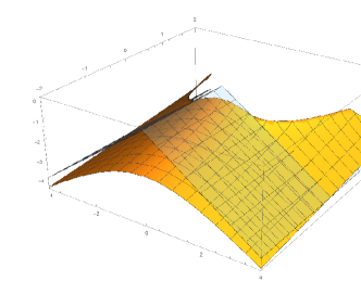
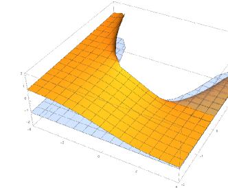
Figure 4.1: Left: The function $(\xi,h)\mapsto{\mathcal{W}}(\xi,h)$ compared with $-|\xi|$. Right: The function ${\mathcal{W}}_{\xi}$ compared with $-1$. In both cases the intersection occurs for $h=0$ and $\xi\geq\overline{\mathfrak{p}}=1$.

5 Discussion

Here we provide some discussion points concerning the notions of evolutionary -convergence. But first in Section 5.1 we highlight that it is important to study the -convergence of ${\mathcal{J}}_{\varepsilon}$ in the weak$\times$strong topology, since using the weak$\times$weak topology results in a smaller dissipation function ${\mathcal{M}}_{\mathrm{w}}$ that is obviously useless, as it does not longer satisfies the estimate ${\mathcal{M}}_{\mathrm{w}}(u,v,\xi)\geq v\xi$. In Section 5.2 we recall the notion of evolutionary -convergence of weak-type introduced in [Vis15]. Also there, it is strongly highlighted that the topology for -convergence needs to be strong enough to make the bilinear mapping $(v,\xi)\mapsto\int_{0}^{T}\langle\xi(t),v(t)\rangle\;\!\mathrm{d}t$ continuous. The last subsections highlight the difference between EDP-convergence and relaxed EDP-convergence.

5.1 -limit in weak$\times$weak topology

We now consider $\mathfrak{J}_{\varepsilon}$ on ${\mathrm{W}}^{1,p}(0,T)\times{\mathrm{L}}^{p^{\prime}}(0,T)$ equipped with the weak$\times$weak topology, which is the natural topology for the family $\mathfrak{J}_{\varepsilon}$ in the sense that is exactly the coarsest topology in which we have equi-coercivity (i.e.  $\mathfrak{J}_{\varepsilon}(u_{\varepsilon},\xi_{\varepsilon})\leq C_{1}$ implies $\|u_{\varepsilon}\|_{{\mathrm{W}}^{1,p}}+\|\xi_{\varepsilon}\|_{{\mathrm{L}}^{p^{\prime}}}\leq C_{2}$). Fortunately, in our wiggly-energy model we have a better convergence for $\xi_{\varepsilon}$ because of the relation $\xi_{\varepsilon}=-{\mathrm{D}}_{u}{\mathcal{E}}_{\varepsilon}(\cdot,u_{\varepsilon})+\Omega_{\varepsilon}(u_{\varepsilon})$, which gave strong convergence.

Here we want to highlight that taking the -limit in the weak$\times$weak topology leads to a functional

$$\mathfrak{J}_{\mathrm{w}}:(u,\xi)\mapsto\int_{0}^{T}{\mathcal{M}}_{\mathrm{w}}(u,\dot{u},\xi)\;\!\mathrm{d}t$$

that is too small. Indeed, using the same techniques as in Section 3 it can be shown that the -limit with respect to this weaker topology is given by

$${\mathcal{M}}_{\mathrm{w}}(u,v,\xi)=\min_{z\in{\mathrm{W}}^{1,p}_{v}(0,1)}\bigg{\{}\int_{0}^{1}{\mathcal{R}}\big{(}u,|v|\dot{z}(s)\big{)}\;\!\mathrm{d}s+{\mathcal{R}}^{*}\Big{(}u,\xi-\int_{0}^{1}\partial_{y}\kappa(u,z(s))\;\!\mathrm{d}s\Big{)}\;\bigg{\}}.$$

We clearly obtain ${\mathcal{M}}_{\mathrm{w}}\leq{\mathcal{M}}$ with ${\mathcal{M}}$ from (1.6). Note that ${\mathcal{M}}_{\mathrm{w}}(u,v,\xi)$ is jointly convex in $(v,\xi)$, so it must be smaller that ${\mathcal{M}}(u,v,\xi)$ in cases where the latter is not convex in $\xi$.

While convexity may be considered as a nice add-on, the lower bound ${\mathcal{M}}_{\mathrm{w}}(u,v,\xi)\geq v\xi$ is essential for the energy-dissipation principle to go back from the energy-dissipation estimate to the subdifferential inclusion. However, ${\mathcal{M}}_{\mathrm{w}}$ does no longer satisfy this important lower bound. To see this, we consider the example ${\mathcal{R}}(u,\dot{u})=\frac{1}{2}\dot{u}^{2}$ and $\kappa(u,y)=a|y|$ for $|y|\leq\frac{1}{2}$ and then periodically extended. Assuming $a,v>0$ and inserting the piecewise interpolant of the points $z(0)=0$, $z(\frac{3}{4})=\frac{1}{2}$, and $z(1)=1$ into the minimization problem defining ${\mathcal{M}}_{\mathrm{w}}$ a simple calculation yields the upper bound ${\mathcal{M}}_{\mathrm{w}}(v,\xi)\leq\frac{2}{3}v^{2}+\frac{1}{2}(\xi-\frac{a}{2})^{2}$. Hence, we obtain ${\mathcal{M}}_{\mathrm{w}}(\frac{a}{2},\frac{a}{2})\leq\frac{1}{6}a^{2}$ which is strictly smaller than $v\xi=\frac{1}{4}a^{2}$.

5.2 Evolutionary $\Gamma$-convergence of weak-type

The definition of EDP-convergence and in particular that of relaxed EDP-convergence is relatively close to the notion of evolutionary $\Gamma$-convergence of the weak-type introduced in [Vis13, Vis15, Vis17a]. There the class of monotone flows in the form

$$\dot{q}+{\bm{A}}(q)\ni\ell(t)$$ (5.1)

are studied, where ${\bm{A}}$ is a maximal monotone operator on an evolution triple ${\bm{Q}}\subset{\bm{H}}\sim{\bm{H}}^{*}\subset{\bm{Q}}^{*}$. The operator ${\bm{A}}$ can be represented in the sense of Fitzpatrick by a function ${\mathcal{G}}:{\bm{Q}}\times{\bm{Q}}^{*}\to{\mathbb{R}}$ as follows:

$${\mathcal{G}}\text{ is convex and }{\mathcal{G}}(q,\xi)\geq\langle\xi,q\rangle\text{ for all }(q,\xi)\in{\bm{Q}}\times{\bm{Q}}^{*},$$

$$\xi\in{\bm{A}}(q)\quad\Longleftrightarrow\quad(q,\xi)\in\mathsf{C}_{\mathcal{G}}=\big{\{}\,(\eta,v)\>\big{|}\>{\mathcal{G}}(v,\eta)=\langle\eta,v\rangle\,\big{\}}.$$

The energy-dissipation principle is replaced by an extended Brezis-Ekeland-Nayroles principle, namely

$$\frac{1}{2}\|q(T)\|_{\bm{H}}^{2}+\mathfrak{G}(q,\ell)=\frac{1}{2}\|q(0)\|_{\bm{H}}^{2},\text{ where }\mathfrak{G}(q,\ell):=\int_{0}^{T}\big{(}{\mathcal{G}}(q,\ell{-}\dot{q})-\langle\ell,q\rangle\big{)}\;\!\mathrm{d}t.$$

For families of monotone flows and associated representation functions ${\mathcal{G}}_{\varepsilon}$ one can then study “static -convergence” for the functionals $\mathfrak{G}_{\varepsilon}$. The applicability of this theory to monotone operators certainly generalizes aspects of our general EDP-convergence in Section 2.2, however it is also more restrictive as these monotone flows are only singly nonlinear, which means for gradient systems $({\bm{Q}},{\mathcal{E}},{\mathcal{R}})$ that ${\mathcal{R}}(q,v)$ cannot depend on $q\in{\bm{Q}}$ and that either ${\mathcal{E}}$ or ${\mathcal{R}}$ are quadratic.

More general classes of pseudo-monotone operators are considered with a further extension of the Brezis–Ekeland–Nayroles principle in [Vis17b].

5.3 Mosco convergence implies EDP-convergence

A simple abstract framework for EDP-convergence can be developed in cases where we have

$${\mathcal{E}}_{\varepsilon}\overset{\Gamma}{\rightharpoonup}{\mathcal{E}}_{0}\quad\text{and}\quad{\mathcal{R}}_{\varepsilon}\overset{\Gamma}{\rightharpoonup}{\mathcal{R}}_{0}.$$

However, these two convergences are certainly not sufficient for EDP-convergence, as they are satisfied in our wiggly-energy model with ${\mathcal{R}}_{0}={\mathcal{R}}$, but $({\mathbb{R}},{\mathcal{E}}_{0},{\mathcal{R}})$ is certainly not the correct limit.

A general abstract theory was developed in [MRS13, Th. 4.8], see also [Mie16, Sec. 3.3.2] for a simplified case and discussion. It relies on the more restrictive notion of Mosco convergence ${\mathcal{F}}_{\varepsilon}\overset{{\mathrm{M}}{\mathrm{o}}}{\longrightarrow}{\mathcal{F}}_{0}$ on a Banach space ${\bm{Q}}$, which means ${\mathcal{F}}_{\varepsilon}\overset{\Gamma}{\to}{\mathcal{F}}_{0}$ and ${\mathcal{F}}_{\varepsilon}\overset{\Gamma}{\rightharpoonup}{\mathcal{F}}_{0}$.

The setup starts from a reflexive Banach space ${\bm{Q}}$ and a densely and compactly embedded energy space ${\bm{Z}}\Subset{\bm{Q}}$. The energies ${\mathcal{E}}_{\varepsilon}:{\bm{Q}}\to{\mathbb{R}}_{\infty}:={\mathbb{R}}\cup\{\infty\}$ are assumed to be equi-coercive in ${\bm{Z}}$ and satisfy ${\mathcal{E}}_{\varepsilon}\overset{\Gamma}{\rightharpoonup}{\mathcal{E}}_{0}$ in ${\bm{Z}}$, which is equivalent to ${\mathcal{E}}\overset{{\mathrm{M}}{\mathrm{o}}}{\longrightarrow}{\mathcal{E}}_{0}$ in ${\bm{Q}}$.

The dissipation potentials ${\mathcal{R}}_{\varepsilon}:{\bm{Z}}\times{\bm{Q}}\to[0,\infty]$ satisfy $p$-equicoercivity with $p>1$:

$$\exists\,c_{1},C_{2},C_{3}>0\ \forall\,\varepsilon\in[0,1]\ \forall\,q\in{\bm{Z}}\ \forall\,v\in{\bm{Q}}:\quad c_{1}\|v\|_{\bm{Q}}^{p}-C_{3}\leq{\mathcal{R}}_{\varepsilon}(q,v)\leq C_{2}\|v\|_{\bm{Q}}^{p}+C_{3}.$$

The convergence of ${\mathcal{R}}_{\varepsilon}$ to ${\mathcal{R}}_{0}$ is the following Mosco convergence:

$$\text{If }q_{\varepsilon}\rightharpoonup q_{0}\text{ in }{\bm{Z}},\ \text{ then }{\mathcal{R}}_{\varepsilon}(q_{\varepsilon},\cdot)\overset{{\mathrm{M}}{\mathrm{o}}}{\longrightarrow}{\mathcal{R}}_{0}(q_{0},\cdot)\text{ in }{\bm{Q}}.$$ (5.2)

Still these conditions are not enough for EDP-convergence (as they hold in our wiggly-energy model), so the crucial additional condition in [MRS13, Thm. 4.8] is the closedness of the subdifferentials of the family $({\mathcal{E}}_{\varepsilon})_{\varepsilon\in[0,1]}$, i.e.

$$\left\{{c}q_{\varepsilon}\to q_{0},\ \xi_{\varepsilon}\rightharpoonup\xi_{*}\text{ in }{\bm{Q}}^{*},\\ \xi_{\varepsilon}\in\partial{\mathcal{E}}_{\varepsilon}(q_{\varepsilon}),\ {\mathcal{E}}_{\varepsilon}(q_{\varepsilon})toE_{0}\right\}\ \Longrightarrow\ \xi_{*}\in\partial{\mathcal{E}}_{0}(q_{0})\text{ and }E_{0}={\mathcal{E}}_{0}(q_{0}).$$

This can be achieved if one has equi-$\lambda$-convexity, i.e. there exists $\lambda_{*}\in{\mathbb{R}}$, such that all functions $q\mapsto{\mathcal{E}}_{\varepsilon}(q)+\lambda_{*}\|q\|_{\bm{Q}}^{2}$ are convex.

If all these conditions (together with some other standard conditions) hold, then one obtains $({\bm{Q}},{\mathcal{E}}_{\varepsilon},{\mathcal{R}}_{\varepsilon})\overset{\mathrm{EDP}}{\longrightarrow}({\bm{Q}},{\mathcal{E}}_{0},{\mathcal{R}}_{0})$. Indeed, in [MRS13, Thm. 4.8] EDP-convergence is not mentioned, however, the proof of evolutionary -convergence is done in a way which exactly shows all ingredients of EDP-convergence.

This is in contrast to the typical Sandier-Serfaty approach [SaS04, Ser11], where only estimates along the precise solutions of the gradient flows are needed.

5.4 EDP-convergence versus relaxed EDP-convergence

More advanced cases of EDP-convergence are discussed in [LM^∗17]. We recall that EDP-convergence distinguishes from relaxed EDP-convergence that the limiting dissipation functional $\mathfrak{D}_{0}$ is given in terms of ${\mathcal{M}}$ having the form

$${\mathcal{M}}(q,v,\xi)={\mathcal{M}}_{\mathrm{eff}}(q,v,\xi):={\mathcal{R}}_{\mathrm{eff}}(q,v)+{\mathcal{R}}^{*}_{\mathrm{eff}}(q,\xi).$$

In the general case this identity is not true, and it is interesting to ask whether we have an estimate of the form ${\mathcal{M}}\geq{\mathcal{M}}_{\mathrm{eff}}$, since only this estimate is needed to show evolutionary -convergence. Yet, for our wiggly-energy model Proposition 4.8 yields the opposite estimate, namely

$${\mathcal{M}}_{\mathrm{eff}}(0,\xi)={\mathcal{R}}_{\mathrm{eff}}^{*}(\xi)>{\mathcal{R}}^{*}(\xi{-}\overline{\mathfrak{p}})=M_{0}(\xi)={\mathcal{M}}(0,\xi)\text{ for all }\xi>\overline{\mathfrak{p}}.$$

Moreover, for $0<v\ll 1$ and $\xi\in[\underline{\mathfrak{p}},\overline{\mathfrak{p}}]$ we have ${\mathcal{M}}(v,\xi)=vM_{1}(\xi)+o(v)_{v\to 0}$ with $M_{1}(\xi)=\int_{0}^{1}|\xi{-}\mathfrak{p}(y)|\;\!\mathrm{d}y$, see Lemma 4.3. For $\xi\in{[0,\overline{\mathfrak{p}}[}$ we have $M_{1}(\xi)<M_{1}(\overline{\mathfrak{p}})=\overline{\mathfrak{p}}$, so we again have ${\mathcal{M}}_{\mathrm{eff}}(v,\xi)=v\overline{\mathfrak{p}}+o(v)>{\mathcal{M}}(v,\xi)=vM_{1}(\xi)+o(v)$.

We feel that this is the typical feature of relaxed EDP-convergence, and conjecture that ${\mathcal{M}}(v,\xi)\leq{\mathcal{M}}_{\mathrm{eff}}$ and that equality holds only in the case of true EDP-convergence. Of course, the difference of ${\mathcal{M}}_{\mathrm{eff}}-{\mathcal{M}}$ always vanishes on the contact set $\mathsf{C}_{\mathcal{M}}$, which highlights that the representation of the operator $v\mapsto\partial{\mathcal{R}}_{\mathrm{eff}}(v)$ can well be given in terms of a function ${\mathcal{M}}$ that is smaller that ${\mathcal{M}}_{\mathrm{eff}}$. We illustrate this by looking at the following special case.

Example 5.1

We want to justify our conjecture by an example calculation for the case ${\mathcal{R}}(v)=\frac{1}{2}v^{2}$ and $\mathfrak{p}$ taking the two values $\pm 1$ with weight $1/2$.

For $\xi>1$ we find ${\mathrm{D}}{\mathcal{R}}^{*}_{\mathrm{eff}}(\xi)=\xi-1/\xi$ and hence ${\mathcal{R}}_{\mathrm{eff}}$ and ${\mathcal{R}}^{*}_{\mathrm{eff}}$ have the form

$${\mathcal{R}}_{\mathrm{eff}}(v)=\frac{1}{4}\big{(}v^{2}+|v|\sqrt{v^{2}{+}4}\big{)}+\mathrm{Asinh}(|v|/2)\ \text{ and }\ {\mathcal{R}}_{\mathrm{eff}}:\xi\mapsto\frac{1}{2}\max\{0,\xi^{2}{-}1\}-\max\{0,\log\xi\}.$$

We can also evaluate ${\mathcal{W}}$ explicitly and find ${\mathcal{W}}(\xi,h)=-\frac{1}{2}\big{(}\sqrt{(\xi{-}1)^{2}-2h}+\sqrt{(\xi{-}1)^{2}-2h}\big{)}$, and Lemma 4.13 gives $\overline{\mathcal{M}}(\xi,h)=h-V(\xi,h){\mathcal{W}}(\xi,h)=h+\sqrt{(\xi{-}1)^{2}-2h}\sqrt{(\xi{-}1)^{2}-2h}$, where $v=V(\xi,h):=1/{\mathcal{W}}_{h}(\xi,h)>0$. Thus, we may check our conjecture for positive $v$, because $v=V(\xi,h)$ tends to $0$ for $h\to-\infty$ and to $\infty$ for $h\nearrow\frac{1}{2}\min\{(\xi{+}1)^{2},(\xi{-}1)^{2}\}$. We can now compare ${\mathcal{M}}$ and ${\mathcal{M}}_{\mathrm{eff}}$ by plotting them over the $(\xi,h)$-plane, and indeed Figure 5.1 shows that the conjecture holds for this simple case.

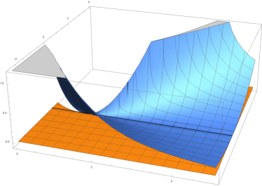
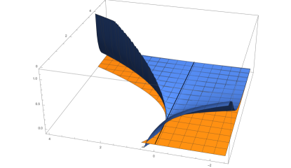
Figure 5.1: Confirmation of the conjecture ${\mathcal{M}}\leq{\mathcal{M}}_{\mathrm{eff}}$ for a special case: The left figure shows that the graph of $(\xi,h)\mapsto{\mathcal{M}}(V(\xi,h),h)-\xi V(\xi,h)$ lies above $0$. The left figure shows that $(\xi,h)\mapsto{\mathcal{M}}_{\mathrm{eff}}(V(\xi,h),h)-{\mathcal{M}}(V(\xi,h)$ lies above $0$. In both cases the functions equal $0$ the bold line $\{\,(\xi,h)\>|\>h=0,\;\xi\geq 1\,\}$. The values for $|\xi|<1$ and $h>0$ are not relevant, because they do not correspond to any $v$.

5.5 Non-convergence of primal and dual dissipation parts

The main observation is that EDP-convergence, and even more relaxed EDP-convergence, are able to work in cases where the nature of the dissipation potential can change its structure. In our wiggly-energy model we found that even though ${\mathcal{R}}_{\varepsilon}={\mathcal{R}}$ we have ${\mathcal{R}}_{\mathrm{eff}}\neq{\mathcal{R}}$. Moreover, for quadratic ${\mathcal{R}}$ we obtain an ${\mathcal{R}}_{\mathrm{eff}}$ that behaves like $v\mapsto\overline{\mathfrak{p}}|v|$ for small $v$.

Such nontrivial changes in the dissipation structure were already observed in [LM^∗17]. For instance it is shown that the diffusion through a layer of thickness $\varepsilon$ with a mobility $a\varepsilon$ has a EDP-limit that describes the jump conditions at a membrane with transmission coefficient $a>0$. The natural gradient structure for diffusion is $({\mathrm{L}}^{1}(\Omega),{\mathcal{E}},{\mathcal{R}}_{\varepsilon})$ with the relative entropy ${\mathcal{E}}(u)=\int_{\Omega}(u\log u-u+1)\;\!\mathrm{d}x$ and the quadratic dissipation potentials of Wasserstein-Kantorovich type, namely

$${\mathcal{R}}_{\varepsilon}^{*}(u,\xi)=\int_{\Omega}\tfrac{A_{\varepsilon}(x)}{2}\,|\nabla\xi(x)|^{2}\,u(x)\;\!\mathrm{d}x$$

The mobility $A_{\varepsilon}$ equals $1$ except for the small layer. It is shown in [Lie12, LM^∗17] that we have EDP-convergence to $({\mathrm{L}}^{1}(\Omega),{\mathcal{E}},{\mathcal{R}}_{\mathrm{eff}})$, and the surprising fact is that ${\mathcal{R}}_{\mathrm{eff}}$ is non-quadratic in $\xi$, because it involves exponential function of the jump of $\xi$ over the limiting membrane.

This change in the structure of the dissipation potentials highlights a general point in EDP-convergence, even when we restrict to exact solutions $q_{\varepsilon}$ of the gradient systems $({\bm{Q}},{\mathcal{E}}_{\varepsilon},{\mathcal{R}}_{\varepsilon})$. Clearly, we have

$${\mathcal{E}}_{\varepsilon}(q_{\varepsilon}(T))+\mathfrak{D}_{\varepsilon}(q_{\varepsilon})={\mathcal{E}}_{\varepsilon}(q_{\varepsilon}(0)).$$

Assume $q_{\varepsilon}(0)\rightharpoonup q_{0}(0)$ and ${\mathcal{E}}_{\varepsilon}(q_{\varepsilon}(0))\to{\mathcal{E}}_{0}(q_{0}(0))$ (i.e. well-prepared initial conditions), the convergence $q_{\varepsilon}\rightharpoonup q_{0}$ in ${\mathrm{W}}^{1,p}(0,T;{\bm{Q}})$ implies

$${\mathcal{E}}_{\varepsilon}(q_{\varepsilon}(t))\to{\mathcal{E}}_{0}(q_{0}(t))\text{ for all }t\in[0,T]\quad\text{and }\mathfrak{D}_{\varepsilon}(q_{\varepsilon})\to\mathfrak{D}_{0}(q_{0}).$$

This means that $q_{\varepsilon}(t)$ is a recovery sequence for the energies ${\mathcal{E}}_{\varepsilon}$ and $q_{\varepsilon}(\cdot)$ is a recovery sequence for the dissipation functionals.

However, the dissipation potential $\mathfrak{D}_{\varepsilon}$ can be understood as the sum of a primal part $\mathfrak{D}_{\varepsilon}^{\mathrm{prim}}$ given via ${\mathcal{R}}_{\varepsilon}$ and of a dual part $\mathfrak{D}_{\varepsilon}^{\mathrm{dual}}$ given via ${\mathcal{R}}^{*}_{\varepsilon}$:

$$\mathfrak{D}_{\varepsilon}^{\mathrm{prim}}(q)=\int_{0}^{T}{\mathcal{R}}_{\varepsilon}(q(t),\dot{q}(t))\;\!\mathrm{d}t\quad\text{and}\quad\mathfrak{D}_{\varepsilon}^{\mathrm{dual}}(q)=\int_{0}^{T}{\mathcal{R}}^{*}_{\varepsilon}\big{(}q(t),{-}{\mathrm{D}}{\mathcal{E}}_{\varepsilon}(q(t))\big{)}\;\!\mathrm{d}t.\quad$$

To understand how the effective dissipation potential ${\mathcal{R}}_{\mathrm{eff}}$ differs from the limits of ${\mathcal{R}}_{\varepsilon}$ we may consider the separate limits

$$\mathsf{D}^{\mathrm{prim}}(q_{0}):=\lim_{\varepsilon\to 0}\mathfrak{D}^{\mathrm{prim}}_{\varepsilon}(q_{\varepsilon})\quad\text{and}\quad\mathsf{D}^{\mathrm{dual}}(q_{0}):=\lim_{\varepsilon\to 0}\mathfrak{D}^{\mathrm{dual}}_{\varepsilon}(q_{\varepsilon})$$

along solutions $q_{\varepsilon}$ of $({\bm{Q}},{\mathcal{E}}_{\varepsilon},{\mathcal{R}}_{\varepsilon})$ converging to a solution $q_{0}$ of $({\bm{Q}},{\mathcal{E}}_{0},{\mathcal{R}}_{\mathrm{eff}})$. Setting

$$\mathfrak{D}_{\mathrm{eff}}^{\mathrm{prim}}(u_{0}):=\int_{0}^{T}{\mathcal{R}}_{\mathrm{eff}}(q_{0},\dot{q}_{0})\;\!\mathrm{d}t\quad\text{and}\quad\mathfrak{D}_{\mathrm{eff}}^{\mathrm{dual}}(u_{0}):=\int_{0}^{T}{\mathcal{R}}^{*}_{\mathrm{eff}}(q_{0},{-}{\mathrm{D}}{\mathcal{E}}_{0}(q_{0}))\;\!\mathrm{d}t.$$

we emphasize that, in general, (relaxed) EDP-convergence does not imply the identities

$$\mathsf{D}^{\mathrm{prim}}(q_{0})=\mathfrak{D}_{\mathrm{eff}}^{\mathrm{prim}}(u_{0})\quad\text{and}\quad\mathsf{D}^{\mathrm{dual}}(q_{0})=\mathfrak{D}_{\mathrm{eff}}^{\mathrm{dual}}(u_{0}).$$ (5.3)

However, for the case considered in Section 5.3 these identities are established in [MRS13, Eqn. (4.29c)] based on the Mosco convergences ${\mathcal{R}}_{\varepsilon}\overset{{\mathrm{M}}{\mathrm{o}}}{\longrightarrow}{\mathcal{R}}_{0}={\mathcal{R}}_{\mathrm{eff}}$, cf. (5.2).

The problems in more general cases are most easily understood when considering $p$-homogenous dissipation potentials ${\mathcal{R}}$ with $p>1$. Then, Euler’s formula gives $\langle\partial{\mathcal{R}}(v),v\rangle=p{\mathcal{R}}(v)$ and $\langle\xi,\partial{\mathcal{R}}^{*}(\xi)\rangle=p^{\prime}{\mathcal{R}}^{*}(\xi)$. Moreover, we have

$$\xi\in\partial{\mathcal{R}}(v)\ \Longrightarrow\ p{\mathcal{R}}(v)={\mathcal{R}}(v){+}{\mathcal{R}}^{*}(\xi)=\langle\xi,v\rangle=p^{\prime}{\mathcal{R}}^{*}(\xi).$$

Thus, if all dissipation potentials ${\mathcal{R}}_{\varepsilon}$ are $p$-homogeneous, we have $\mathfrak{D}^{\mathrm{prim}}_{\varepsilon}(q_{\varepsilon})=\frac{1}{p}\mathfrak{D}_{\varepsilon}(q_{\varepsilon})$ and $\mathfrak{D}^{\mathrm{dual}}_{\varepsilon}(q_{\varepsilon})=\frac{1}{p^{\prime}}\mathfrak{D}_{\varepsilon}(q_{\varepsilon})$, and the convergence of $\mathfrak{D}_{\varepsilon}(q_{\varepsilon})\to\mathfrak{D}_{0}(q_{0})$ yields

$$\mathsf{D}^{\mathrm{prim}}(q_{0})=\frac{1}{p}\mathfrak{D}_{0}(q_{0})\text{ and }\mathsf{D}^{\mathrm{dual}}(q_{0})=\frac{1}{p^{\prime}}\mathfrak{D}_{0}(q_{0}).$$

Of course, by (relaxed) EDP-convergence we have the representation

$$\mathfrak{D}_{0}(q_{0})=\int_{0}^{T}{\mathcal{M}}(q_{0},\dot{q}_{0},{-}{\mathrm{D}}{\mathcal{E}}(q_{0}))\;\!\mathrm{d}t=\mathfrak{D}_{\mathrm{eff}}^{\mathrm{prim}}(q_{0})+\mathfrak{D}_{\mathrm{eff}}^{\mathrm{dual}}(q_{0}).$$

Here the second identity follows since $q_{0}$ is a solutions such that $(\dot{q}_{0},{-}{\mathrm{D}}{\mathcal{E}}_{0}(q_{0}))$ lies in $\mathsf{C}_{\mathcal{M}}$, where ${\mathcal{M}}$ equals ${\mathcal{M}}_{\mathrm{eff}}$, as both functional equal $\langle\xi,v\rangle$ on $\mathsf{C}_{\mathcal{M}}$.

The question as to whether the two identities in (5.3) hold is now reduced to the question whether ${\mathcal{R}}_{\mathrm{eff}}(q,\cdot)$ is still $p$-homogeneous. Thus, in the Sandier-Serfaty approach, where $p=2$ for $\varepsilon>0$ as well as for $\varepsilon=0$, we have the desired identity.

However, in our wiggly-energy model we can start with arbitrary $p>1$ for $\varepsilon>0$ but end up with ${\mathcal{R}}_{\mathrm{eff}}$ satisfying $\langle\partial{\mathcal{R}}_{\mathrm{eff}}(u,v),v\rangle=\alpha(u,v){\mathcal{R}}_{\mathrm{eff}}(v)$ with $\alpha(u,v)\in{[1,p[}$, see Proposition 4.10. Hence, we obtain a strict inequality, namely

$$\mathsf{D}^{\mathrm{prim}}(u_{0})\ =\ \frac{1}{p}\mathfrak{D}_{0}(u_{0})\ =\ \frac{1}{p}\int_{0}^{T}\big{(}{\mathcal{R}}_{\mathrm{eff}}(u_{0},\dot{u}_{0})+{\mathcal{R}}^{*}_{\mathrm{eff}}(u_{0},{-}{\mathrm{D}}{\mathcal{E}}_{0}(u_{0}))\big{)}\;\!\mathrm{d}t$$

$$=\ \frac{1}{p}\int_{0}^{T}\!\!\partial_{v}{\mathcal{R}}_{\mathrm{eff}}(u_{0},\dot{u}_{0})\dot{u}_{0}\;\!\mathrm{d}t\ =\ \int_{0}^{T}\!\!\frac{\alpha(u_{0},\dot{u}_{0})}{p}{\mathcal{R}}_{\mathrm{eff}}(u_{0},\dot{u}_{0})\;\!\mathrm{d}t\ \lneqq\ \int_{0}^{T}\!{\mathcal{R}}_{\mathrm{eff}}(u_{0},\dot{u}_{0})\;\!\mathrm{d}t.$$

Because $\alpha(u,0)=1$ the effect is stronger if $\dot{u}_{0}$ is small, i.e. when we are close to the rate-independent case.

In the membrane limit of thin layers discussed in [Lie12, LM^∗17] we have quadratic dissipation potentials for $\varepsilon>0$, i.e. $p=2$. However, for $\varepsilon=0$ one obtains ${\mathcal{R}}_{\mathrm{eff}}$ with a growth like $|v|\log|v|$ for $|v|\gg 1$. Again we have $\langle\partial{\mathcal{R}}_{\mathrm{eff}}(\dot{q}),\dot{q}\rangle=b(\dot{q}){\mathcal{R}}_{\mathrm{eff}}(\dot{q})$, where $b(\dot{q})\leq 2$ and $b(\dot{q})<2$ for certain $\dot{q}$. However, there the effect is stronger for large $\dot{q}$ and disappears for $\dot{q}\to 0$.

For both cases we see that in the limiting primal part of the dissipation functional $\int_{0}^{T}{\mathcal{R}}_{\mathrm{eff}}(q_{0},\dot{q}_{0})\;\!\mathrm{d}t$ is larger than the limit $\mathsf{D}^{\mathrm{prim}}(q_{0})=\lim_{\varepsilon\to 0}\mathfrak{D}^{\mathrm{prim}}_{\varepsilon}(q_{\varepsilon})$. This is also seen in the inequality ${\mathcal{R}}_{\varepsilon}\overset{\Gamma}{\rightharpoonup}{\mathcal{R}}_{0}\leq{\mathcal{R}}_{\mathrm{eff}}$. We interpret this as the effect of microscopic dissipative processes that need to be modeled on the macroscale for the limit system $({\bm{Q}},{\mathcal{E}}_{0},{\mathcal{R}}_{\mathrm{eff}})$.

It is an interesting question to understand whether relaxed EDP-convergence always leads to an increase for the primal part of the dissipation functional; more precisely, do we always have $\mathsf{D}^{\mathrm{prim}}(q_{0})\leq\int_{0}^{T}{\mathcal{R}}_{\mathrm{eff}}(q_{0},\dot{q}_{0})\;\!\mathrm{d}t$?

References

• [AbK88] R. Abeyaratne and J. K. Knowles. On the dissipative response due to discontinuous strains in bars of unstable elastic material. Internat. J. Solids Structures, 24(10), 1021–1044, 1988.
• [AbK97] R. Abeyaratne and J. K. Knowles. On the kinetics of an austenite $\rightarrow$ martensite phase transformation induced by impact in a CuAlNi shape-memory alloy. Acta Materialia, 45(4), 1671 – 1683, 1997.
• [ACJ96] R. Abeyaratne, C.-H. Chu, and R. James. Kinetics of materials with wiggly energies: theory and application to the evolution of twinning microstructures in a Cu-Al-Ni shape memory alloy. Phil. Mag. A, 73, 457–497, 1996.
• [AGS05] L. Ambrosio, N. Gigli, and G. Savaré. Gradient flows in metric spaces and in the space of probability measures. Lectures in Mathematics ETH Zürich. Birkhäuser Verlag, Basel, 2005.
• [Att84] H. Attouch. Variational Convergence of Functions and Operators. Pitman Advanced Publishing Program. Pitman, 1984.
• [BdV08a] M. Buliga, G. de Saxcé, and C. Valleé. Existence and construction of bipotentials for graphs of multivalued laws. J. Convex Anal., 15(1), 87–104, 2008.
• [BdV08b] M. Buliga, G. de Saxcé, and C. Valleé. Non maximal cyclically monotone graphs and construction of a bipotential for the Coulomb’s dry friction law. arXiv:0802.1140v1, 2008.
• [Bha99] K. Bhattacharya. Phase boundary propagation in a heterogeneous body. R. Soc. Lond. Proc. Ser. A Math. Phys. Eng. Sci., 455(1982), 757–766, 1999.
• [BoP16] G. A. Bonaschi and M. A. Peletier. Quadratic and rate-independent limits for a large-deviations functional. Contin. Mech. Thermodyn., 28(4), 1191–1219, 2016.
• [Bra02] A. Braides. $\Gamma$-Convergence for Beginners. Oxford University Press, 2002.
• [Bra13] A. Braides. Local minimization, Variational Evolution and Gamma-convergence. Lect. Notes Math. Vol. 2094. Springer, 2013.
• [Bud17] M. Buliga and G. de Saxcé. A symplectic Brezis-Ekeland-Nayroles principle. Math. Mech. Solids, 22(6), 1288–1302, 2017.
• [Dal93] G. Dal Maso. An Introduction to $\Gamma$-Convergence. Birkhäuser Boston Inc., Boston, MA, 1993.
• [DKW17] P. W. Dondl, M. W. Kurzke, and S. Wojtowytsch. The Effect of Forest Dislocations on the Evolution of a Phase-Field Model for Plastic Slip. arXiv.org, July 2017.
• [DMT80] E. De Giorgi, A. Marino, and M. Tosques. Problems of evolution in metric spaces and maximal decreasing curve. Atti Accad. Naz. Lincei Rend. Cl. Sci. Fis. Mat. Natur. (8), 68(3), 180–187, 1980.
• [EfM06] M. Efendiev and A. Mielke. On the rate–independent limit of systems with dry friction and small viscosity. J. Convex Anal., 13(1), 151–167, 2006.
• [EkT76] I. Ekeland and R. Temam. Convex Analysis and Variational Problems. North Holland, 1976.
• [EsC93] J. Escobar and R. Clifton. On pressure-shear plate impact for studying the kinetics of stress-induced phase transformations. Materials Science and Engineering: A, 170(1), 125 – 142, 1993.
• [Fen49] W. Fenchel. On conjugate convex functions. Canadian J. Math., 1, 73–77, 1949.
• [GaM05] A. Garroni and S. Müller. $Gamma$-limit of a phase-field model of dislocations. SIAM Journal on Mathematical Analysis, 36(6), 1943–1964 (electronic), 2005.
• [GaM06] A. Garroni and S. Müller. A variational model for dislocations in the line tension limit. Archive For Rational Mechanics And Analysis, 181(3), 535–578, 2006.
• [GiD17] P. Gidoni and A. DeSimone. On the genesis of directional friction through bristle-like mediating elements crawler. ESAIM Control Optim. Calc. Var., 23(3), 1023–1046, 2017.
• [Jam96] R. D. James. Hysteresis in phase transformations. In ICIAM 95 (Hamburg, 1995), volume 87 of Math. Res., pages 135–154. Akademie Verlag, Berlin, 1996.
• [Lie12] M. Liero. Variational Methods for Evolution. PhD thesis, Institut für Mathematik, Humboldt-Universität zu Berlin, 2012.
• [LM17] M. Liero, A. Mielke, M. A. Peletier, and D. R. M. Renger. On microscopic origins of generalized gradient structures. Discr. Cont. Dynam. Systems Ser. S, 10(1), 1–35, 2017.
• [LMS17] M. Liero, A. Mielke, and G. Savaré. Optimal entropy-transport problems and the Hellinger–Kantorovich distance. Invent. math., 2017. Accepted. WIAS preprint 2207, arXiv:1508.07941v2.
• [Men02] G. Menon. Gradient systems with wiggly energies and related averaging problems. Arch. Rat. Mech. Analysis, 162, 193–246, 2002.
• [Mie11] A. Mielke. Complete-damage evolution based on energies and stresses. Discr. Cont. Dynam. Systems Ser. S, 4(2), 423–439, 2011.
• [Mie12] A. Mielke. Emergence of rate-independent dissipation from viscous systems with wiggly energies. Contin. Mech. Thermodyn., 24(4), 591–606, 2012.
• [Mie16] A. Mielke. On evolutionary $\Gamma$-convergence for gradient systems (Ch. 3). In A. Muntean, J. Rademacher, and A. Zagaris, editors, Macroscopic and Large Scale Phenomena: Coarse Graining, Mean Field Limits and Ergodicity, Lecture Notes in Applied Math. Mechanics Vol. 3, pages 187–249. Springer, 2016. Proc. of Summer School in Twente University, June 2012.
• [MiT12] A. Mielke and L. Truskinovsky. From discrete visco-elasticity to continuum rate-independent plasticity: rigorous results. Arch. Rational Mech. Anal., 203(2), 577–619, 2012.
• [MoM77] L. Modica and S. Mortola. Un esempio di $\Gamma$-convergenza. Boll. Un. Mat. Ital. B, 14, 285–299, 1977.
• [MoP12] R. e. Monneau and S. Patrizi. Homogenization of the Peierls-Nabarro model for dislocation dynamics. Journal of Differential Equations, 253(7), 2064–2105, 2012.
• [MPR14] A. Mielke, M. A. Peletier, and D. R. M. Renger. On the relation between gradient flows and the large-deviation principle, with applications to Markov chains and diffusion. Potential Analysis, 41(4), 1293–1327, 2014.
• [MRS09] A. Mielke, R. Rossi, and G. Savaré. Modeling solutions with jumps for rate-independent systems on metric spaces. Discr. Cont. Dynam. Systems Ser. A, 25(2), 585–615, 2009.
• [MRS12] A. Mielke, R. Rossi, and G. Savaré. BV solutions and viscosity approximations of rate-independent systems. ESAIM Control Optim. Calc. Var., 18(1), 36–80, 2012.
• [MRS13] A. Mielke, R. Rossi, and G. Savaré. Nonsmooth analysis of doubly nonlinear evolution equations. Calc. Var. Part. Diff. Eqns., 46(1-2), 253–310, 2013.
• [MRS16] A. Mielke, R. Rossi, and G. Savaré. Balanced-viscosity (BV) solutions to infinite-dimensional rate-independent systems. J. Europ. Math. Soc., 18, 2107–2165, 2016.
• [PoG12] V. L. Popov and J. A. T. Gray. Prandtl-Tomlinson model: History and applications in friction, plasticity, and nanotechnologies. Z. angew. Math. Mech. (ZAMM), 92(9), 692–708, 2012.
• [Pra28] L. Prandtl. Gedankenmodel zur kinetischen Theorie der festen Körper. Z. angew. Math. Mech. (ZAMM), 8, 85–106, 1928.
• [PRV14] M. A. Peletier, F. Redig, and K. Vafayi. Large deviations in stochastic heat-conduction processes provide a gradient-flow structure for heat conduction. J. Math. Physics, 55, 093301/19, 2014.
• [PuT02a] G. Puglisi and L. Truskinovsky. A mechanism of transformational plasticity. Contin. Mech. Thermodyn., 14, 437–457, 2002.
• [PuT02b] G. Puglisi and L. Truskinovsky. Rate independent hysteresis in a bi-stable chain. J. Mech. Phys. Solids, 50(2), 165–187, 2002.
• [PuT05] G. Puglisi and L. Truskinovsky. Thermodynamics of rate-independent plasticity. J. Mech. Phys. Solids, 53, 655–679, 2005.
• [Roc70] R. T. Rockafellar. Convex Analysis. Princeton University Press, 1970.
• [SaS04] E. Sandier and S. Serfaty. Gamma-convergence of gradient flows with applications to Ginzburg-Landau. Comm. Pure Appl. Math., LVII, 1627–1672, 2004.
• [Ser11] S. Serfaty. Gamma-convergence of gradient flows on Hilbert spaces and metric spaces and applications. Discr. Cont. Dynam. Systems Ser. A, 31(4), 1427–1451, 2011.
• [SK09] T. J. Sullivan, M. Koslowski, F. Theil, and M. Ortiz. On the behaviour of dissipative systems in contact with a heat bath: Application to andrade creep. J. Mech. Phys. Solids, 57(7), 1058–1077, 2009.
• [Ste08] U. Stefanelli. The Brezis-Ekeland principle for doubly nonlinear equations. SIAM J. Control Optim., 47(3), 1615–1642, 2008.
• [Sul09] T. J. Sullivan. Analysis of Gradient Descents in Random Energies and Heat Baths. PhD thesis, Dept. of Mathematics, University of Warwick, 2009.
• [Tom29] G. A. Tomlinson. A molecular theory of friction. Philos. Mag., 7, 905–939, 1929.
• [Vis13] A. Visintin. Variational formulation and structural stability of monotone equations. Calc. Var. Part. Diff. Eqns., 47, 273–317, 2013.
• [Vis15] A. Visintin. Structural stability of flows via evolutionary $\Gamma$-convergence of weak-type. arxiv:1509:03819, 2015.
• [Vis17a] A. Visintin. Evolutionary $\Gamma$-convergence of weak type. arXiv:1706.02172, pages 1–8, 2017.
• [Vis17b] A. Visintin. Structural compactness and stability of pseudo-monotone flows. arXiv:1706.02176, 2017.