Asymmetric melting of one-third plateau in kagome quantum antiferromagnets

Abstract

Asymmetric destruction of the one-third magnetization plateau upon heating is found in the spin-1/2 kagome Heisenberg antiferromagnets using the typical pure quantum state approach. The asymmetry originates from a larger density of states of low-lying excited states of $N_{\rm s}$ spin systems with magnetization $(1/3-2/N_{\rm s})$ than that of low-lying states with magnetization $(1/3+2/N_{\rm s})$. The enhanced specific heat and entropy that reflect the larger density of states in the lower-field side of the plateau are detectable in candidate materials of the kagome antiferromagnets. We discuss that the asymmetry originates from the unprecedented preservation of the ice rule around the plateau.

I Introduction

Interplay between the geometrical frustrations and the quantum fluctuations often prohibits spontaneous symmetry breakings and induces quantum spin liquid states in many-body quantum spins. The spin-1/2 antiferromagnet on the kagome lattice is one of the promising candidates of the quantum spin liquids and intensive theoretical studies have been done  Jiang et al. (2008); Lu et al. (2011); Yan et al. (2011); Depenbrock et al. (2012); Jiang et al. (2012); Nishimoto et al. (2013); Läuchli et al. (2016); Ran et al. (2007); Nakano and Sakai (2011); Iqbal et al. (2015); He et al. (2017). Although recent highly-accurate simulations show that the long-range magnetic order is absent in the kagome lattice, it is still under hot debate what kind of the quantum spin liquid (e.g. gapped $Z_{2}$ spin liquid Jiang et al. (2008); Lu et al. (2011); Yan et al. (2011); Depenbrock et al. (2012); Jiang et al. (2012); Nishimoto et al. (2013); Läuchli et al. (2016) or gapless $U(1)$ Dirac spin liquid Ran et al. (2007); Nakano and Sakai (2011); Iqbal et al. (2015); He et al. (2017)) is realized.

The magnetization process of the kagome Heisenberg model has attracted much interest because the magnetization plateaus under magnetic fields show exotic orders Zhitomirsky (2002); Hida (2001); Zhitomirsky and Tsunetsugu (2004); Nakano and Sakai (2010); Nishimoto et al. (2013); Picot et al. (2016). Recent theoretical calculations have shown that the one-third magnetization plateau appears in the spin-1/2 kagome Heisenberg model Hida (2001); Nishimoto et al. (2013); Capponi et al. (2013); Picot et al. (2016). The detailed exact diagonalization study, however, claims that the one-third plateau is not conventional plateau by examining the critical exponents of the magnetization process Nakano and Sakai (2010); Sakai and Nakano (2011); Nakano and Sakai (2014). It is also an unresolved issue what kind of magnetic order realizes in the one-third plateau because different magnetic orders are suggested Nishimoto et al. (2013); Picot et al. (2016).

Because the one-third magnetization plateau is characteristic of the candidate materials for the kagome antiferromagnets Ishikawa et al. (2015), it is an important issue to clarify how the finite-temperature effects stabilize or destabilize the one-third plateau. Although finite-temperature properties at zero magnetic field have been studied by several numerical methods Elstner and Young (1994); Misguich and Sindzingre (2007); Sindzingre (2007); Misguich and Bernu (2005); Nakamura and Miyashita (1995); Sugiura and Shimizu (2013); Shimokawa and Kawamura (2016), finite-temperature properties under magnetic fields such as the finite-temperature magnetization are not systematically examined.

In this paper, we study the thermodynamics of the antiferromagnetic Heisenberg model on the kagome lattice under magnetic fields by using the TPQ state method Sugiura and Shimizu (2012) that enables us to calculate thermodynamics of the quantum many-body systems including the kagome antiferromagnets Sugiura and Shimizu (2013); Shimokawa and Kawamura (2016) in an unbiased way. We note that similar methods were proposed in the pioneering works Imada and Takahashi (1986); Hams and De Raedt (2000); Jaklič and Prelovšek (1994). We focus on the finite-temperature effects around the one-third magnetization plateau.

As a result, we have found that the peculiar asymmetric collapse of the one-third plateau occurs at finite temperatures. This asymmetric collapse can be explained by the large degeneracy existing just below the plateau. We will discuss that the asymmetric degeneracy can be explained by the preservation of the ice rule. In the one-third plateau, we have shown that the $\sqrt{3}\times\sqrt{3}$ magnetic order is realized at the ground state but several apparent disordered states compete with the $\sqrt{3}\times\sqrt{3}$ order, which is consistent with previous studies Honecker et al. (2005); Cabra et al. (2005); Picot et al. (2016). Reflecting the anomalous degeneracies, the entropy remains large even at the plateau down to the lowest temperatures. We have also found that the enhancement of the entropy and the specific heat just below the plateau appears, which can be detected experimentally.

This paper is organized as follows: In Sec. II, we introduce the antiferromagnetic Heisenberg model on the kagome lattice and explains the details of the TPQ method. In Sec. III, we show the results of the finite-temperature effects on the one-third magnetization plateau. In Sec. IV, we analyze the low-energy excited states around the one-third magnetization plateau by using the locally optimal block conjugate gradient (LOBCG) method. In Sec. V, we show results of the magnetic field dependence of the thermodynamic properties such as the entropy and the specific heat. Sec. VI is devoted to the summary and discussions.

II Model and Methods

We study the antiferromagnetic Heisenberg model on the kagome lattice defined as

$${\cal H} =J\sum_{\langle i,j\rangle}\boldsymbol{S}_{i}\cdot\boldsymbol{S}_{j}-h\sum_{i}S_{i}^{z}$$ (1)

where $\boldsymbol{S}_{i}$ is a spin operator of the localized spin-1/2 at $i$th site and $h$ denotes the magnetic field. The antiferromagnetic interactions $J>0$ only exist between the nearest-neighbor sites $\langle i,j\rangle$ on the kagome lattice. The magnetization $m$ is defined as $m=\frac{1}{SN_{\rm s}}\sum_{i}\langle S_{i}^{z}\rangle$, where $N_{\rm s}$ is the number of the sites and we take $S=1/2$. In this definition, saturation magnetization is given by $m_{\rm s}=1$. We mainly analyze 27 site and 36 site clusters for the kagome lattice with a periodic boundary condition in the present paper. For comparison, we perform the calculations for the triangular lattice (27 site clusters), which also has the one-third plateau under magnetic fields.

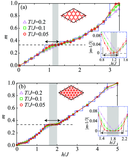
Figure 1: (color online). Finite-temperature magnetization process of the spin-1/2 antiferromagnetic Heisenberg model (a) on the kagome lattice and (b) the triangular lattice. The magnetization at $T=0$ is also shown by a solid line. In the left insets, the lattice structures for 36 site kagome lattice and 27 site triangular lattice are shown. The one-third plateau region ($m=1/3$ within error bars) at $T/J=0.05$ is shown by the shaded region. The arrow shows the region where the one-third plateau appears at zero temperature for $N_{\rm s}=36$ (kagome lattice) and $N_{\rm s}=27$ (triangular lattice). In the right insets, we show $|m-1/3|$ around the plateaus for both lattices.

In this paper, we use the TPQ state to analyze the finite-temperature properties. In the TPQ method, we iteratively generate the $k$th TPQ state as

$$|\psi_{k}\rangle\equiv\frac{(l-\hat{\cal{H}}/N_{\rm s})|\psi_{k-1}\rangle}{|(l-\hat{\cal{H}}/N_{\rm s})|\psi_{k-1}\rangle|},$$ (2)

where $|\psi_{0}\rangle$ is an initial random wavefunction and $l$ is a constant that is larger than the maximum eigenvalue of ${\cal{H}}/N_{\rm s}$ Sugiura and Shimizu (2012). In this study, we typically take $l/J=3$. From the $k$th TPQ state, we can calculate thermodynamic properties such as temperature, internal energy, and the spin correlations Sugiura and Shimizu (2012); Kawamura et al. (2017). To examine properties of the ground state and low-energy excited states, we also perform the LOBCG method Knyazev (2001).

Here, we mention about the limitation of the TPQ method. Although the TPQ method gives the unbiased and essentially exact results for given finite system sizes, the errors of the TPQ method, which are defined by the standard deviations of the statistical distribution of the initial random vectors $|\psi_{0}\rangle$, is bounded by the residual entropy Sugiura and Shimizu (2012, 2013). If the residual entropy is large, the errors of the TPQ method become smaller, i.e., the initial vector dependence of the physical quantities becomes small. Thus, in the previous works Sugiura and Shimizu (2013); Yamaji et al. (2014); Shimokawa and Kawamura (2016); Misawa and Yamaji (2018); Laurell and Okamoto (2020), the TPQ method is used for examining the finite-temperature properties of the quantum spin liquid where the large remaining entropy is expected. As shown in Appendix A, for s small system size, we confirm that the TPQ method well reproduces the result obtained by the full diagonalization (see Fig. 5). We note that the average values of the physical quantities become exact in the limit of a large number of samplings when we independently evaluate the averages of the distribution function and the physical quantities, as is done in the canonical TPQ method Sugiura and Shimizu (2013).

In the following calculations, we evaluate the error bars of the TPQ calculations by choosing several independent initial vectors. As we show later, in the relevant temperature region ($T\geq 0.05$), the errors of the TPQ calculations are small. We can safely discuss the finite-temperature effects on the 1/3 plateau in the kagome lattice.

III Finite-temperature effects on the one-third magnetization plateau

In Fig. 1(a) and (b), we show the finite-temperature magnetization process of the Heisenberg model on the kagome lattice and the triangular lattice. To see the finite-temperature effects on the one-third plateaus, we show the width of the one-third plateaus at zero temperature as arrows for both lattices.

At high temperature ($T/J=0.2$), the magnetization changes smoothly as a function of the magnetic field for both lattices. By lowering the temperature, a plateau-like structure appears around $h/J=1.2$ in the kagome lattice and $h/J=1.8$ in the triangular lattice (see the right insets in Fig.1). We, however, find that the width of the plateau in the kagome lattice is largely different from that of the zero-temperature limit even at the lowest temperature ($T/J=0.05$), while the width of the plateau in the triangular lattice seems to smoothly converge to the zero-temperature limit. The asymmetric behavior in the kagome lattice indicates that the low-energy excitations above and below the one-third plateau are different, i.e., the density of states for the lower-field side is larger than the density of states for the higher-field side. We will confirm that the asymmetric structure exists in the low-energy excited states. We note that error bars around the 1/3 plateau in the kagome lattice are large, and this may originate from the peculiar degeneracy in the 1/3 plateau, as we will discuss later.

In Fig. 2(a), we show that the temperature dependence of the magnetization in the kagome lattice for several different magnetic fields. Dashed vertical lines show the temperatures where we plot the magnetization process in Fig. 1(a). When the temperature is decreased, the magnetization converges to $m=1/3$ around $h/J=1.2$, which indicates the formation of the plateau at the finite temperature. As shown in Fig. 2(b), we confirm that the magnetization converges to $m=1/3$ at low temperatures around $h/J=1.2$.

As we mentioned above, around $h/J=0.9$, the plateau appears at zero temperature while it vanishes at finite temperatures ($T/J=0.05$). As shown in Fig. 2(c), because we find that finite-size effects are small at $h/J=0.9$, it is plausible that the fragility of the magnetization plateau at a low magnetic field side is intrinsic phenomena.

In addition to the one-third plateau around $h/J=1.2$, we find that the apparent magnetization plateau ($m=14/36$) exists slightly above the one-third plateau, i.e., around $h/J=1.6$ as shown in Figs. 2(a) and (c). Because the system size dependence of the apparent plateau is large, as shown in Fig. 2(c), the additional plateau seems to be an artifact of the finite-size effects and may vanish in the thermodynamic limit. The apparent magnetization originates from the “ramp” structure observed in zero-temperature calculations, where the magnetization smoothly converges to the plateau above the one-third plateau Nakano and Sakai (2010). In finite-size systems, this ramp structure induces the apparent plateau due to the discreteness of the magnetization.

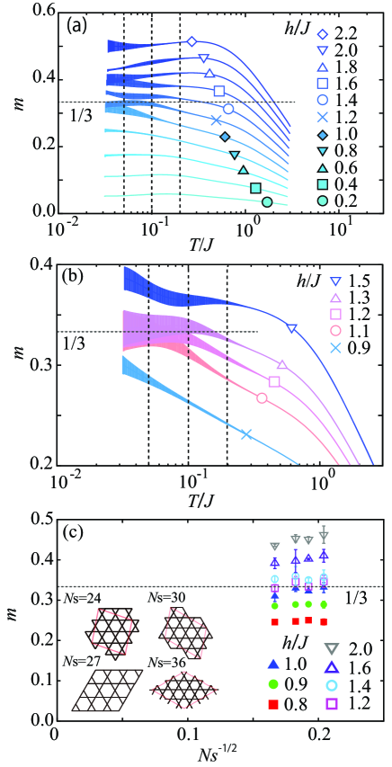
Figure 2: (color online).  (a) Temperature dependence of the magnetization in the kagome lattice (36 site clusters) for several different magnetic fields. Around $h/J=1.2$, magnetization saturates to $1/3$. Slightly above the one-third plateau, we also find the signature of another apparent plateau around $h/J=1.6$. However, we conclude that this plateau is induced by the finite-size effects as we discussed in the main text. (b) Temperature dependence of the magnetization around the $1/3$ plateau. For $h/J=1.1,1.2,$ and $1.3$, the magnetizations converge to 1/3 at low temperatures. (c) Size-dependence of the magnetization at $T/J=0.05$ for different magnetic fields. We take $N_{\rm s}=24,27,30$, and $36$ clusters. In the insets, the shapes of the used clusters are shown. The size-dependent error bars around 1/3 plateau may originate from the peculiar degeneracy in the 1/3 plateau.

IV Low-energy excitations around the one-third plateau

Here, we examine the low-energy excitations around the plateau by using LOBCG method Knyazev (2001). In the inset of Fig. 3(a), we show the lowest 128 eigenvalues for the 27 site cluster and the lowest 16 eigenenergies for the 36 site cluster around the plateau. Irrespective of the system sizes, we find a large density of states exists just below the plateau, i.e., $m=7/27$ ($m=10/36$) for the 27 (36) site clusters. We define the density of states as the number of eigenstates per unit energy $J$. As we show, we confirm that the slope of the magnetization curve (susceptibility) is proportional to the density of states, i.e., $\frac{\partial m}{\partial h}\propto{\rm(density~{}of~{}states)}$ For the 27 site clusters, all the 128 eigenenergies exist within $0.2J$ from the ground states. In sharp contrast to this, the density of states is small just above the plateau [$m=11/27$ (27 sites) and $m=14/36$ (36 sites)]. We note that the large density of states is consistent with the anomalous steep magnetization process just below the plateau, which is pointed out in the previous studies Nakano and Sakai (2010); Sakai and Nakano (2011); Nakano and Sakai (2014). This can be rephrased as the difference of the degeneracy induces the ramp structure in the magnetization process Nakano and Sakai (2010), i.e., the large degeneracy below the plateau induces the steep change in the magnetization and small degeneracy above the plateau induces the small slope in magnetization process.

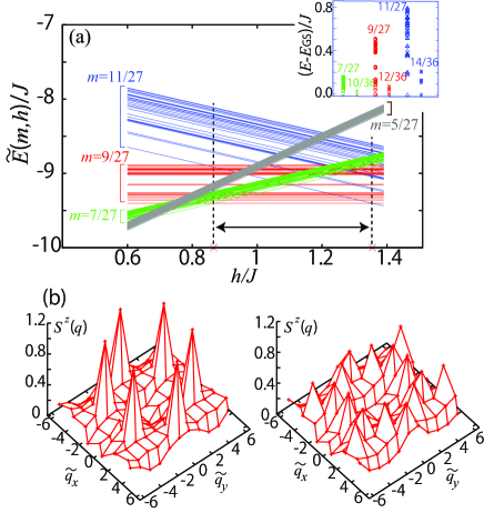
Figure 3: (color online).  (a) Low-energy spectrum around the one-third magnetization plateau for the 27 site cluster. We plot $\tilde{E}(m,h)=E(m)-h\times(m-1/3)$ for $m=7/27,9/27=1/3,11/27$. Dotted lines show the position of the crossing points of the lowest energies. The arrow indicates the width of the plateau at zero temperature. In the inset, we show the lowest 128 eigenenergies for 27 site clusters ($m={5/27},7/27,9/27,11/27$) and the lowest 16 eigenenergies for 36 site clusters ($m=10/36,12/36,14/36$). The eigenenergies are measured from the ground-state energy $E_{\rm GS}$. (b) Spin structure factors in the extended Brillouin zone for the 36 site cluster at $m=1/3$ for the ground state (left panel) and the third excited state (right panel), where $\tilde{q}_{\alpha}=q_{\alpha}\times\frac{3}{\pi}~{}(\alpha=x,y)$. In the ground state, there are sharp peaks at $\boldsymbol{q}=(\pm 4\pi/3,0),(\pm 2\pi/3,\pm 2\pi/\sqrt{3})$, which correspond to the $\sqrt{3}\times\sqrt{3}$ order. In contrast to that, we find no significant peaks in the spin structure factor in the third excited state whose energy difference is given by $E_{\rm third}-E_{\rm GS}\sim 0.04J$.

To see how the asymmetric low-energy excitations affect the finite-temperature magnetization process, we plot the magnetic field dependence of the low-energy spectrum $\tilde{E}(m,h)=E(m)-h(m-1/3)$ in Fig. 3(a). Because the degeneracy between different $m$ sectors, i.e., $m=1/3$ and $m=7/27$, exists around the lower endpoint of the plateau $h/J\sim 0.8$, the different magnetizations can be easily mixed by the finite-temperature effects. We also point out that $m=5/27$ can largely affect the lower bound of the plateau as shown in Fig. 3(a). This is the reason why the plateau is destroyed around $h/J\leq 0.9$ even at the lowest temperature $T/J=0.05$. In contrast to that, around the higher endpoint of the plateau ($h/J\sim 1.2$), the degeneracy is weak and the magnetization plateau is robust against the finite-temperature effects.

In Fig. 3(b), we show the spin structure factors $S^{z}(\boldsymbol{q})$, which is defined as

$$S^{z}(\boldsymbol{q})=\frac{1}{N_{\rm s}}\sum_{i,j}e^{{\rm i}\boldsymbol{q}(\boldsymbol{r}_{i}-\boldsymbol{r}_{j})}(S_{i}^{z}-\langle S_{i}^{z}\rangle)(S_{j}^{z}-\langle S_{j}^{z}\rangle),$$ (3)

where $r_{i}$ denotes the position of the lattice point in the two dimensions. We find that spin structure factors have sharp peaks at $\boldsymbol{q}=(\pm 4\pi/3,0),(\pm 2\pi/3,\pm 2\pi/\sqrt{3})$ in the ground state. This indicates that the $\sqrt{3}\times\sqrt{3}$ spin structures realize in the ground state. We also find that the several excited states that do not show any signature of magnetically ordered states compete with the $\sqrt{3}\times\sqrt{3}$ orders (see the right panel in Fig. 3(b)). One of the candidates of the apparent disordered state is the nematic state. Further detailed analysis of the nature of the disordered state is left for future studies. This result indicates that degeneracy still exists even in the plateau region Cabra et al. (2005); Picot et al. (2016). As we show later, this degeneracy induces the large remaining entropy at low temperature.

V Magnetic-field dependence of entropy and specific heat

In Fig. 4(a), we show the temperature dependence of the specific heat $C$, which is defined as

$$C=\frac{\langle H^{2}\rangle-\langle H\rangle^{2}}{N_{\rm s}T^{2}}.$$ (4)

At $h=0$, we obtain the same temperature dependence of the specific heat in the previous studies Sugiura and Shimizu (2013); Shimokawa and Kawamura (2016). We find that the shoulder structure at $h/J=0$ below $T/J\sim 0.2$, which roughly corresponds to the singlet-triplet excitation gap Waldtmann et al. (1998); Nakano and Sakai (2011), is immediately vanished by applying the magnetic field ($h/J=0.2$). Thus, as shown in Fig. 4(b), the entropy at finite temperatures ($T/J\leq 0.1$), which is defined as

$${S(T)=1-\frac{1}{\rm ln2}\int_{T}^{\infty}\frac{C}{T}\mathrm{d}T},$$ (5)

increases when the magnetic fields are applied. In the plateau region, the entropy is relatively low but the entropy is not fully released down to the lowest temperature $T/J=0.05$. This result is consistent with the fact that the degeneracy still exists in the plateau.

We show the magnetic-field dependence of the specific heat coefficient $C/T$ in Fig. 4(c). Just below the one-third plateau, we find the enhancement of $C/T$, which is consistent with the degeneracy existing in the low-energy excited state. This large enhancement of $C/T$ is the characteristic feature of the plateau in the kagome lattice and is expected to be detected in experiments. We note that the behaviors of the specific heat around the saturation field (peaks and dip around $h/J=3$) are consistent with those of the hard hexagon model Zhitomirsky and Tsunetsugu (2004), which well describes the low-energy degrees of freedom of the quantum kagome Heisenberg model around the saturation field.

Here, we clarify the origin of the asymmetric plateau melting and the difference in the density of states for $m=1/3-2/N_{\rm s}$ and $m=1/3+2/N_{\rm s}$ in the kagome-lattice Heisenberg model. The asymmetry originates from the ice-rule configuration of spins around the one-third plateau. As shown in the inset of Fig. 4(b), the ground-state and low-lying excited-state wave functions show a large probability of adhering to the ice rule at $m=1/3$ for the kagome lattice while the probability is relatively low for the triangular lattice. Therefore, we can assume that the spin configurations for $m\sim 1/3$ are generated by keeping the ice-rule constraint as much as possible. Under the constraint, there are $N_{\rm s}/3$ ($2N_{\rm s}/3$) flippable spins to increment (decrement) the total $S^{z}$ from the one-third plateau by 1. This asymmetry is the origin of the asymmetric plateau melting. The degeneracy lifting by the kinetic energy of a defect (flipped spin) in the ice manifold for $m=1/3+2/N_{\rm s}$ may explain the smaller entropy for $m>1/3$ than that for the $m=1/3$ state. We note that the preservation of the ice-rule is consistent with the fact that the one-third plateau at the Heisenberg point has a large overlap with its Ising limit Cabra et al. (2005).

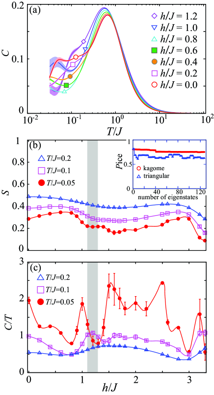
Figure 4: (color online).  (a) Temperature dependence of the specific heat for several different magnetic fields. (b) Magnetic field dependence of the entropy $S$ for several different temperatures. The region where the one-third plateau appears at $T/J=0.05$ is represented by the shaded region. In the inset, we show the probability of the ice rule $P_{\rm ice}$ for 128 eigenstates in 27 site clusters. $P_{\rm ice}$ is defined in Appendix B. (c) Magnetic-field dependence of the specific heat $C/T$ for several different temperatures. At $T/t=0.05$, we find that $C/T$ has peaks at both the sides of the one-third plateau. We note that the finite-size effects are small around the one-third plateau for both $S$ and $C/T$. Solid curves are guides for eyes.

VI Summary and Discussions

In summary, we analyze the thermodynamic properties of the spin-1/2 antiferromagnetic Heisenberg model on the kagome lattice by using the TPQ method. We show that the one-third magnetization plateau in the kagome lattice is asymmetrically destroyed at finite temperatures.

By using the LOBCG method, we show that the large degeneracy exists just below the plateau. The degeneracy induces the asymmetric behavior and the enhancement of both the entropy and the specific heat. We also identify that the origin of the degeneracy is the unexpected robustness of the ice-rule configurations at the plateau. Our detailed and unbiased analyses on the thermodynamics of the ideal quantum kagome antiferromagnets under magnetic fields offer a firm basis for characterizing the experimental candidates of the kagome antiferromagnets Ishikawa et al. (2015); Hiroi et al. (2001); Shores et al. (2005); Mendels and Bert (2010); Okamoto et al. (2009, 2011).

Recently, it is shown that we can treat up to 50-site systems by reducing the size of Hilbert dimensions using the symmetries inherent in systems Wietek and Läuchli (2018). By taking such large system size, we can obtain a more definitive conclusion on the anomalous thermodynamic properties on the 1/3 plateau. We note that it is also a challenging problem to study the temperature dependence of the static and dynamical spin correlation function based on the TPQ method Yamaji et al. (2018). Further investigations along this direction are intriguing but left for future studies.

Note added.— Recently, we became aware of independent numerical work Chen et al. (2018) that treats the finite-temperature properties of the kagome-lattice Heisenberg model but focuses on a different aspect. We also became aware that the similar asymmetric melting was independently reported in Ref. [Schnack et al., 2018] after submitting the article.

Appendix A Comparison with full diagonalization

Here, we examine the accuracy of the TPQ method by comparing with the result obtained by the full diagonalization. In Fig. 5, for 18-site kagome lattice with total $S_{z}=0$ (dimension of the Hilbert space is 48620), we show the temperature dependence of the energy obtain by the TPQ method and the full diagonalization. From this result, we confirm that the TPQ method well reproduces exact results.

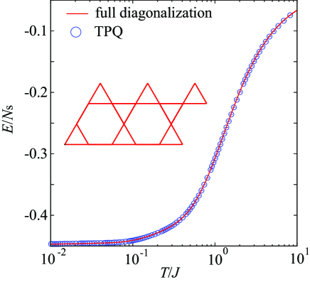
Figure 5: (color online). Temperature dependence of the energy obtained by the TPQ method (blue circles) and the full diagonalization (red curve). For the TPQ calculations, we perform 5 independent runs and regard its standard deviation as error bars. In the inset, we show the geometry used in the calculation.

Appendix B Definitions of ice rule

In this appendix, we show the definitions of the ice rule. We defined the local measure of the ice rule on one upper triangular defined as

$$n_{\triangle} =\frac{1}{3}\left\{\left(S^{z}_{\triangle(1)}-\frac{1}{2}\right)\left(S^{z}_{\triangle(2)}-\frac{1}{2}\right)\left(S^{z}_{\triangle(3)}+\frac{1}{2}\right)\right.$$ (6)

$$\quad+\left(S^{z}_{\triangle(1)}-\frac{1}{2}\right)\left(S^{z}_{\triangle(2)}+\frac{1}{2}\right)\left(S^{z}_{\triangle(3)}-\frac{1}{2}\right)$$ (7)

$$\quad+\left.\left(S^{z}_{\triangle(1)}+\frac{1}{2}\right)\left(S^{z}_{\triangle(2)}-\frac{1}{2}\right)\left(S^{z}_{\triangle(3)}-\frac{1}{2}\right)\right\}$$ (8)

$$=S^{z}_{\triangle(1)}S^{z}_{\triangle(2)}S^{z}_{\triangle(3)}$$

$$\quad-\frac{1}{6}\left(S^{z}_{\triangle(1)}S^{z}_{\triangle(2)}+S^{z}_{\triangle(2)}S^{z}_{\triangle(3)}+S^{z}_{\triangle(3)}S^{z}_{\triangle(1)}\right)$$ (9)

$$\quad-\frac{1}{12}\left(S^{z}_{\triangle(1)}+S^{z}_{\triangle(2)}+S^{z}_{\triangle(3)}\right)$$

$$\quad+\frac{1}{8},$$

where $S^{z}_{\triangle(i)}$ is the $z$ component of the spin operator $S^{z}$ at the $i$th site of the upper triangle. We note how to index the three sites on the triangular does not affect because these sites are equivalent.

By using this $n_{\triangle}$, we calculate $P_{\rm ice}$ as follows:

$$\Delta =\sum_{\triangle}n_{\triangle},$$ (10)

$$P_{\rm ice} =\frac{1}{N_{\rm norm}}\sum_{i}|a_{i}|^{2}\langle i|\Delta|i\rangle,$$ (11)

where $a_{i}$ is a coefficient of the $i$th real-space configuration $|i\rangle$, $\Delta$ is number of upward triangles that satisfy the ice rule, and $N_{\rm norm}$ is defined for $P_{\rm ice}$ becomes one when the ice rule is completely satisfied. We note that $P_{\rm ice}\sim 0.4707$ ($N_{\rm s}=27$) for a random configuration of spins irrespective of the lattice geometry.

References

- Jiang et al. (2008) H. C. Jiang, Z. Y. Weng, and D. N. Sheng, Phys. Rev. Lett. 101, 117203 (2008).
- Lu et al. (2011) Y.-M. Lu, Y. Ran, and P. A. Lee, Phys. Rev. B 83, 224413 (2011).
- Yan et al. (2011) S. Yan, D. A. Huse, and S. R. White, Science 332, 1173 (2011).
- Depenbrock et al. (2012) S. Depenbrock, I. P. McCulloch, and U. Schollwöck, Phys. Rev. Lett. 109, 067201 (2012).
- Jiang et al. (2012) H.-C. Jiang, Z. Wang, and L. Balents, Nat. Phys. 8, 902 (2012).
- Nishimoto et al. (2013) S. Nishimoto, N. Shibata, and C. Hotta, Nat. Commun. 4, 2287 (2013).
- Läuchli et al. (2016) A. M. Läuchli, J. Sudan, and R. Moessner, arXiv:1611.06990 (2016).
- Ran et al. (2007) Y. Ran, M. Hermele, P. A. Lee, and X.-G. Wen, Phys. Rev. Lett. 98, 117205 (2007).
- Nakano and Sakai (2011) H. Nakano and T. Sakai, J. Phys. Soc. Jpn. 80, 053704 (2011).
- Iqbal et al. (2015) Y. Iqbal, D. Poilblanc, and F. Becca, Phys. Rev. B 91, 020402(R) (2015).
- He et al. (2017) Y.-C. He, M. P. Zaletel, M. Oshikawa, and F. Pollmann, Phys. Rev. X 7, 031020 (2017).
- Zhitomirsky (2002) M. E. Zhitomirsky, Phys. Rev. Lett. 88, 057204 (2002).
- Hida (2001) K. Hida, J. Phys. Soc. Jpn. 70, 3673 (2001).
- Zhitomirsky and Tsunetsugu (2004) M. E. Zhitomirsky and H. Tsunetsugu, Phys. Rev. B 70, 100403(R) (2004).
- Nakano and Sakai (2010) H. Nakano and T. Sakai, J. Phys. Soc. Jpn. 79, 053707 (2010).
- Picot et al. (2016) T. Picot, M. Ziegler, R. Orús, and D. Poilblanc, Phys. Rev. B 93, 060407(R) (2016).
- Capponi et al. (2013) S. Capponi, O. Derzhko, A. Honecker, A. M. Läuchli, and J. Richter, Phys. Rev. B 88, 144416 (2013).
- Sakai and Nakano (2011) T. Sakai and H. Nakano, Phys. Rev. B 83, 100405(R) (2011).
- Nakano and Sakai (2014) H. Nakano and T. Sakai, J. Phys. Soc. Jpn. 83, 104710 (2014).
- Ishikawa et al. (2015) H. Ishikawa, M. Yoshida, K. Nawa, M. Jeong, S. Krämer, M. Horvatić, C. Berthier, M. Takigawa, M. Akaki, A. Miyake, et al., Phys. Rev. Lett. 114, 227202 (2015).
- Elstner and Young (1994) N. Elstner and A. P. Young, Phys. Rev. B 50, 6871 (1994).
- Misguich and Sindzingre (2007) G. Misguich and P. Sindzingre, Euro. Phys. J. B 59, 305 (2007).
- Sindzingre (2007) P. Sindzingre, arXiv:0707.4264 (2007).
- Misguich and Bernu (2005) G. Misguich and B. Bernu, Phys. Rev. B 71, 014417 (2005).
- Nakamura and Miyashita (1995) T. Nakamura and S. Miyashita, Phys. Rev. B 52, 9174 (1995).
- Sugiura and Shimizu (2013) S. Sugiura and A. Shimizu, Phys. Rev. Lett. 111, 010401 (2013).
- Shimokawa and Kawamura (2016) T. Shimokawa and H. Kawamura, J. Phys. Soc. Jpn. 85, 113702 (2016).
- Sugiura and Shimizu (2012) S. Sugiura and A. Shimizu, Phys. Rev. Lett. 108, 240401 (2012).
- Imada and Takahashi (1986) M. Imada and M. Takahashi, J. Phys. Soc. Jpn. 55, 3354 (1986).
- Hams and De Raedt (2000) A. Hams and H. De Raedt, Phys. Rev. E 62, 4365 (2000).
- Jaklič and Prelovšek (1994) J. Jaklič and P. Prelovšek, Phys. Rev. B 49, 5065 (1994).
- Honecker et al. (2005) A. Honecker, D. Cabra, M. Grynberg, P. Holdsworth, P. Pujol, J. Richter, D. Schmalfua, and J. Schulenburg, Physica B: Condensed Matter 359-361, 1391 (2005).
- Cabra et al. (2005) D. C. Cabra, M. D. Grynberg, P. C. W. Holdsworth, A. Honecker, P. Pujol, J. Richter, D. Schmalfuß, and J. Schulenburg, Phys. Rev. B 71, 144420 (2005).
- Kawamura et al. (2017) M. Kawamura, K. Yoshimi, T. Misawa, Y. Yamaji, S. Todo, and N. Kawashima, Comput. Phys. Commun. 217, 180 (2017).
- Knyazev (2001) A. V. Knyazev, SIAM journal on scientific computing 23, 517 (2001).
- Yamaji et al. (2014) Y. Yamaji, Y. Nomura, M. Kurita, R. Arita, and M. Imada, Phys. Rev. Lett. 113, 107201 (2014).
- Misawa and Yamaji (2018) T. Misawa and Y. Yamaji, Journal of the Physical Society of Japan 87, 023707 (2018).
- Laurell and Okamoto (2020) P. Laurell and S. Okamoto, npj Quantum Materials 5 (2020).
- Waldtmann et al. (1998) C. Waldtmann, H.-U. Everts, B. Bernu, C. Lhuillier, P. Sindzingre, P. Lecheminant, and L. Pierre, Eur. Phys. J. B 2, 501 (1998).
- Hiroi et al. (2001) Z. Hiroi, M. Hanawa, N. Kobayashi, M. Nohara, H. Takagi, Y. Kato, and M. Takigawa, J. Phys. Soc. Jpn. 70, 3377 (2001).
- Shores et al. (2005) M. P. Shores, E. A. Nytko, B. M. Bartlett, and D. G. Nocera, J. Am. Chem. Soc. 127, 13462 (2005).
- Mendels and Bert (2010) P. Mendels and F. Bert, J. Phys. Soc. Jpn. 79, 011001 (2010).
- Okamoto et al. (2009) Y. Okamoto, H. Yoshida, and Z. Hiroi, J. Phys. Soc. Jpn. 78, 033701 (2009).
- Okamoto et al. (2011) Y. Okamoto, M. Tokunaga, H. Yoshida, A. Matsuo, K. Kindo, and Z. Hiroi, Phys. Rev. B 83, 180407(R) (2011).
- Wietek and Läuchli (2018) A. Wietek and A. M. Läuchli, Physical Review E 98, 033309 (2018).
- Yamaji et al. (2018) Y. Yamaji, T. Suzuki, and M. Kawamura, arXiv preprint arXiv:1802.02854 (2018).
- Chen et al. (2018) X. Chen, S.-J. Ran, T. Liu, C. Peng, Y.-Z. Huang, and G. Su, Science Bulletin 63, 1545 (2018).
- Schnack et al. (2018) J. Schnack, J. Schulenburg, and J. Richter, Phys. Rev. B 98, 094423 (2018).
- hph (a) http://www.pasums.issp.u-tokyo.ac.jp/HPhi/.
- hph (b) https://github.com/issp-center-dev/HPhi.