Bootstrapping hypercubic and hypertetrahedral
theories in three dimensions

Abstract

There are three generalizations of the Platonic solids that exist in all dimensions, namely the hypertetrahedron, the hypercube, and the hyperoctahedron, with the latter two being dual. Conformal field theories with the associated symmetry groups as global symmetries can be argued to exist in $d=3$ spacetime dimensions if the $\varepsilon=4-d$ expansion is valid when $\varepsilon\to 1$. In this paper hypercubic and hypertetrahedral theories are studied with the non-perturbative numerical conformal bootstrap. In the $N=3$ cubic case it is found that a bound with a kink is saturated by a solution with properties that cannot be reconciled with the $\varepsilon$ expansion of the cubic theory. Possible implications for cubic magnets and structural phase transitions are discussed. For the hypertetrahedral theory evidence is found that the non-conformal window that is seen with the $\varepsilon$ expansion exists in $d=3$ as well, and a rough estimate of its extent is given.

1 Introduction

The numerical conformal bootstrap [1] in three dimensions has produced impressive results, especially concerning critical theories in universality classes that also contain scalar conformal field theories (CFTs). For the Ising universality class the bootstrap is in fact the state-of-the-art method for the determination of critical exponents [2, 3, 4, 5]. For theories with continuous global symmetries there has also been significant progress, with important developments for the Heisenberg universality class [6, 7, 8]. In this work we study critical theories with discrete global symmetries in three dimensions, focusing on the hypercubic and hypertetrahedral symmetry groups.

The motivation for our considerations is twofold. First, in the cubic case with $N=3$ scalar fields the issue of its stability relative to the $O(3)$ theory has, to our knowledge, remained unresolved; see [9, 10] and references therein. Second, in the hypertetrahedral case there exists a non-conformal window, at least as far as the $\varepsilon$ expansion is concerned [11, 12], meaning that there is a range of the number $N$ of scalar fields for which there are no hypertetrahedral fixed points, while such fixed points can be found below and above that range. In this paper we study these questions directly in $d=3$ with the bootstrap by considering a single four-point function, namely that of the scalar operator $\phi_{i},i=1,\ldots,N$.

To our knowledge there have been no non-perturbative Monte Carlo studies of hypercubic or hypertetrahedral CFTs in $d=3$, although the cubic deformation at the $O(3)$ fixed point has been studied with Monte Carlo methods in [13]. The standard lore (see e.g. [9]) is thus mostly based on the perturbative $\varepsilon=4-d$ expansion [14] with the use of resummation techniques [15, 16]. The $\varepsilon$ expansion has proven to be quite powerful in the $O(N)$ and Ising models, among others. Nevertheless, it is hard to argue rigorously and in generality about its effectiveness in $d=3$, or $\varepsilon=1$. Therefore, it is very important to check the results of the $\varepsilon$ expansion whenever non-perturbative methods are available. In this paper we attempt to do this for hypercubic and hypertetrahedral theories using the bootstrap. Our expectation is that the predictions of the $\varepsilon$ expansion should persist beyond perturbation theory. Various results for the hypercubic and hypertetrahedral theories obtained with the $\varepsilon$ expansion were recently summarized in [12]. Many quantitative results for the hypercubic theory can be found in [9] and references therein, while some newer results can be found in [17], notably pertaining to non-singlet and non-scalar operators.

One aim of this work is to provide general bounds on scaling dimensions of operators in hypercubic and hypertetrahedral theories. In some cases these bounds are found to display kinks. In the bootstrap we typically think of kinks as special positions in parameter space where the bounds are saturated by actual theories. We are also interested in bounds on OPE coefficients, especially the central charge. Such bounds also display features that we attribute to saturation from actual CFTs.

In this work we find that the solution of crossing that saturates a certain bound with a kink (Fig. 2 below) has properties that do not agree with the $\varepsilon$ expansion. To be more specific, we are referring to the $N=3$ case, where our bootstrap results show that the first singlet scalar, i.e. what one would call the “$\phi^{2}$” operator, has scaling dimension that differs significantly between the $O(3)$ fixed point and the solution at the kink, called $C_{3}^{b}$ here. The $\varepsilon$ expansion indicates that the “$\phi^{2}$” operator should have more or less the same scaling dimension both at the $O(3)$ and the cubic theory $C_{3}^{\varepsilon}$ accessed with it [18, 19, 9].

Furthermore, when we study the stability of the $C_{3}^{b}$ solution, we find another surprise. Based on the $\varepsilon$ expansion results of [20] it is expected that, if it exists, the stable fixed point under a given set of deformations is unique. From our bootstrap analysis we find that the $C_{3}^{b}$ solution is stable, i.e. it has only one relevant scalar singlet operator (namely the “$\phi^{2}$” operator). Now, stable fixed points should describe physical systems at second order phase transitions reached by tuning the temperature. However, in cubic magnets, where the cubic deformation is important, the critical exponents appear to take the $O(3)$ or $C_{3}^{\varepsilon}$ values according to experiments [9]. Since we find the critical exponents of the $C_{3}^{b}$ solution to be very different from those of the $C_{3}^{\varepsilon}$ and $O(3)$ models, we see that despite the fact that the $C_{3}^{b}$ solution is stable, it is the $O(3)$ or $C_{3}^{\varepsilon}$ theory that describes cubic magnets at criticality. From these observations one concludes that neither the $C_{3}^{b}$ solution nor one of the $O(3)$ or $C_{3}^{\varepsilon}$ theories has a second relevant operator, directly contradicting the perturbative result of [20]. To our knowledge there is no contradiction with having two stable fixed points non-perturbatively.

Our solution $C_{3}^{b}$ appears unrelated to the $C_{3}^{\varepsilon}$ theory found with the $\varepsilon$ expansion. We are unable to determine if the $C_{3}^{b}$ solution at the kink corresponds to an actual CFT. Perhaps it does not, in which case the kink is an artifact of the numerics. $C_{3}^{b}$ could also correspond to a theory with cubic symmetry that cannot be obtained with the $\varepsilon$ expansion. We are unable to settle this question in this work.

For the hypertetrahedral theories we find that our non-perturbative results are consistent with the perturbative ones. Focusing on the non-conformal window, we find that its range as estimated with the bootstrap is reasonably close to that obtained with the $\varepsilon$ expansion. We should note, however, that our bootstrap determination is approximate. We expect that more accurate results can be obtained by considering a mixed-correlator bootstrap.

The structure of the paper is as follows. In the next section we outline some group theory that allows us to obtain the hypercubic crossing equation. In section 3 we use the numerical bootstrap method to find operator dimension bounds in various sectors of hypercubic theories, analyze the spectrum of the solution at a bound, and discuss extensively possible implications of our results both for cubic magnets and for structural phase transitions. We also obtain bounds on the central charge. In section 4 we derive the hypertetrahedral crossing equation. Finally, in section 5 we get operator dimension bounds in hypertetrahedral theories and comment on the non-conformal window. We conclude in section 6. In an appendix we perform a bootstrap analysis of the cubic crossing equation in $d=3.8$.

Note Added: While this manuscript was in preparation [21] appeared which also considered the bootstrap with hypertetrahedral symmetry. There is a small overlap of their results with ours in sections 4 and 5.

2 Hypercubic symmetry

For the hypercubic (or hyperoctahedral since hypercubes are dual to hyperoctahedra) group at $N=4$ useful references include [22, 23]. For general $N$ a useful reference is [24].

To start, let us go through the $N=3$ cubic symmetry group in some detail. In Coxeter notation this is the group $C_{3}$ (or $B_{3}$). It is given by the semi-direct product $\mathcal{S}_{3}\ltimes\mathbb{Z}_{2}{}^{3}\simeq\mathcal{S}_{4}\ltimes\mathbb{Z}_{2}$, where $\mathcal{S}_{n}$ is the permutation group of $n$ elements. $C_{3}$ is a subgroup of $O(3)$. The group $O(3)$ keeps the dot product of two arbitrary three-vectors invariant. If these vectors have integer coefficients in the canonical $\mathbb{R}^{3}$ basis, then $C_{3}$ also preserves that property. This statement generalizes to $C_{N}=S_{N}\ltimes\mathbb{Z}_{2}{}^{N}$ [24], which has $2^{N}N!$ elements.

The irreducible representations of $C_{3}$ are those of $\mathcal{S}_{4}$ (for each parity due to the $\mathbb{Z}_{2}$), which are known to be the $\boldsymbol{1},\bar{\boldsymbol{1}},\boldsymbol{2},\boldsymbol{3}$ and $\bar{\boldsymbol{3}}$. If $C_{3}$ is viewed as a subgroup of $O(3)$, it is the traceless symmetric representation of $O(3)$ that gives rise to the representations $\boldsymbol{2}$ and $\bar{\boldsymbol{3}}$. Terms that belong to the diagonal make up the $\boldsymbol{2}$, while off-diagonal terms give rise to the $\bar{\boldsymbol{3}}$. $\bar{\boldsymbol{1}}$ is the one-dimensional sign representation, taking into account only the signature of the permutation. Finally, $\boldsymbol{1}$ is the trivial representation and $\boldsymbol{3}$ corresponds to the antisymmetric representation. For our purposes operators exchanged in the $\phi_{i}\times\phi_{j}$ OPE need to be considered. There are singlets of even spin and antisymmetric tensors of odd spin, and, instead of traceless symmetric operators of even spin as in the $O(3)$ case, there are operators of even spin in the $\boldsymbol{2}$ and $\bar{\boldsymbol{3}}$ of $C_{3}$.

It turns out that many statements in the previous paragraph generalize to the $C_{N}$ case. For example, the singlet and antisymmetric representation of $O(N)$ remain irreducible under $C_{N}$ [24], while the traceless-symmetric representation of $O(N)$ splits into two irreducible representations under $C_{N}$, furnished separately by diagonal and off-diagonal terms.

In the case of $O(N)$ symmetry the four-point function $\langle\phi_{i}(x_{1})\phi_{j}(x_{2})\phi_{k}(x_{3})\phi_{l}(x_{4})\rangle$ was decomposed in conformal blocks in [25, 6]. In the $12\to 34$ channel, for example,

$$\begin{split}x_{12}^{2\Delta_{\phi}}x_{34}^{2\Delta_{\phi}}\langle\phi_{i}(x_{1})\phi_{j}(x_{2})\phi_{k}(x_{3})\phi_{l}(x_{4})\rangle&=\sum_{\text{S}^{+}_{\mathbin{\scalerel*{\bigcirc}{t}}}}\lambda_{\mathcal{O}}^{2}\hskip 1.0pt\delta_{ij}\delta_{kl}\hskip 1.0ptg_{\Delta,\hskip 1.0pt\ell}(u,v)\\ &\quad+\sum_{\text{T}^{+}_{\mathbin{\scalerel*{\bigcirc}{t}}}}\lambda_{\mathcal{O}}^{2}\hskip 1.0pt\Big{(}\delta_{ik}\delta_{jl}+\delta_{il}\delta_{jk}-\frac{2}{N}\delta_{ij}\delta_{kl}\Big{)}\hskip 1.0ptg_{\Delta,\hskip 1.0pt\ell}(u,v)\\ &\quad+\sum_{\text{A}^{-}_{\mathbin{\scalerel*{\bigcirc}{t}}}}\lambda_{\mathcal{O}}^{2}\hskip 1.0pt(\delta_{ik}\delta_{jl}-\delta_{il}\delta_{jk})\hskip 1.0ptg_{\Delta,\hskip 1.0pt\ell}(u,v)\,,\end{split}$$ (2.1)

where three classes of operators contribute, namely even-spin singlets, even-spin traceless-symmetric tensors, and odd-spin antisymmetric tensors, as follows from the representation theory of $O(N)$. In the hypercubic case the first and the last term in (2.1) remain the same, but the middle term gets further decomposed under the hypercubic group. In particular, the diagonal terms, with $i=j$ and $k=l$, need to be distinguished from the non-diagonal terms.

To proceed we introduce the tensors

$$A_{ijkl}=\delta_{ijkl}\,,\qquad B_{ijkl}=\delta_{ij}\delta_{kl}-\delta_{ijkl}\,,\qquad\delta_{ijkl}=\begin{cases}1,&i=j=k=l\\ 0,&\text{otherwise}\end{cases}\,.$$ (2.2)

The tensor $B_{ijkl}$ is only symmetric under $i\leftrightarrow j$, $k\leftrightarrow l$ and $ij\leftrightarrow kl$. This allows us to separate the diagonal terms, with $i=j$ and $k=l$, from the non-diagonal terms in (2.1). Indeed, using (2.2) equation (2.1) can be decomposed to the hypercubic form

$$\begin{split}x_{12}^{2\Delta_{\phi}}x_{34}^{2\Delta_{\phi}}\langle\phi_{i}(x_{1})\phi_{j}(x_{2})\phi_{k}(x_{3})\phi_{l}(x_{4})\rangle&=\sum_{\text{S}_{\square}^{+}}\,\lambda_{\mathcal{O}}^{2}\hskip 1.0pt(A_{ijkl}+B_{ijkl})\hskip 1.0ptg_{\Delta,\hskip 1.0pt\ell}(u,v)\\ &\quad+\sum_{\text{V}_{\square}^{+}}\lambda_{\mathcal{O}}^{2}\hskip 1.0pt\bigg{(}\Big{(}2-\frac{2}{N}\Big{)}A_{ijkl}-\frac{2}{N}B_{ijkl}\bigg{)}\hskip 1.0ptg_{\Delta,\hskip 1.0pt\ell}(u,v)\\ &\quad+\sum_{\text{Y}_{\square}^{+}}\lambda_{\mathcal{O}}^{2}\hskip 1.0pt(B_{ikjl}+B_{iljk})\hskip 1.0ptg_{\Delta,\hskip 1.0pt\ell}(u,v)\\ &\quad+\sum_{\text{A}_{\square}^{-}}\lambda_{\mathcal{O}}^{2}\hskip 1.0pt(B_{ikjl}-B_{iljk})\hskip 1.0ptg_{\Delta,\hskip 1.0pt\ell}(u,v)\,,\end{split}$$ (2.3)

where there are now four classes of operators that contribute, since the even-spin $\text{T}^{+}_{\mathbin{\scalerel*{\bigcirc}{t}}}$ operators of (2.1) decompose into the $\text{V}_{\square}^{+}$ and $\text{Y}_{\square}^{+}$ operators under hypercubic symmetry. Equation (2.3) has appeared already in [17].

The hypercubic crossing equation can be derived by exchanging $(1,i)\leftrightarrow(3,k)$, collecting terms that multiply the same tensor structure, and symmetrizing/antisymmetrizing in $u,v$. Defining

$$F_{\Delta,\hskip 1.0pt\ell}^{\pm}(u,v)=v^{\Delta_{\phi}}g_{\Delta,\hskip 1.0pt\ell}(u,v)\pm u^{\Delta_{\phi}}g_{\Delta,\hskip 1.0pt\ell}(v,u)\,,$$ (2.4)

we find

$$\sum_{\text{S}_{\square}^{+}}\lambda_{\mathcal{O}}^{2}\begin{pmatrix}0\\ F^{-}_{\Delta,\hskip 1.0pt\ell}\\ F^{+}_{\Delta,\hskip 1.0pt\ell}\\ F^{-}_{\Delta,\hskip 1.0pt\ell}\end{pmatrix}+\sum_{\text{V}_{\square}^{+}}\lambda_{\mathcal{O}}^{2}\begin{pmatrix}0\\ -\tfrac{2}{N}F^{-}_{\Delta,\hskip 1.0pt\ell}\\ -\tfrac{2}{N}F^{+}_{\Delta,\hskip 1.0pt\ell}\\ (2-\tfrac{2}{N})F^{-}_{\Delta,\hskip 1.0pt\ell}\end{pmatrix}+\sum_{\text{Y}_{\square}^{+}}\!\lambda_{\mathcal{O}}^{2}\begin{pmatrix}F^{-}_{\Delta,\hskip 1.0pt\ell}\\ F^{-}_{\Delta,\hskip 1.0pt\ell}\\ -F^{+}_{\Delta,\hskip 1.0pt\ell}\\ 0\end{pmatrix}+\sum_{\text{A}_{\square}^{-}}\lambda_{\mathcal{O}}^{2}\begin{pmatrix}F^{-}_{\Delta,\hskip 1.0pt\ell}\\ -F^{-}_{\Delta,\hskip 1.0pt\ell}\\ F^{+}_{\Delta,\hskip 1.0pt\ell}\\ 0\end{pmatrix}=\begin{pmatrix}0\\ 0\\ 0\\ 0\end{pmatrix}.$$ (2.5)

Compared to the $O(N)$ case we have one more crossing equation for the hypercubic theory.

Another way to derive the hypercubic crossing equation is to recall the presence of a rank-four traceless-symmetric primitive invariant tensor $d_{ijkl}$ in theories with hypercubic symmetry, satisfying [12]

$$d_{ijmn}d_{mnkl}=\frac{N}{(N+2)^{2}}\Big{(}\delta_{ik}\delta_{jl}+\delta_{il}\delta_{jk}-\frac{2}{N}\delta_{ij}\delta_{kl}\Big{)}+\frac{N-2}{N+2}\hskip 1.0ptd_{ijkl}\,.$$ (2.6)

We can then define the linearly-independent invariant projectors

$$\begin{split}P_{ijkl}^{(1)}&=\frac{1}{N}\delta_{ij}\delta_{kl}\,,\\ P_{ijkl}^{(2)}&=d_{ijkl}+\frac{1}{N+2}\Big{(}\delta_{ik}\delta_{jl}+\delta_{il}\delta_{jk}-\frac{2}{N}\delta_{ij}\delta_{kl}\Big{)}\,,\\ P_{ijkl}^{(3)}&=-d_{ijkl}+\frac{N}{2(N+2)}\Big{(}\delta_{ik}\delta_{jl}+\delta_{il}\delta_{jk}-\frac{2}{N}\delta_{ij}\delta_{kl}\Big{)}\,,\\ P_{ijkl}^{(4)}&=-\tfrac{1}{2}(\delta_{ik}\delta_{jl}-\delta_{il}\delta_{jk})\,,\end{split}$$ (2.7)

that satisfy

$$P_{ijmn}^{(I)}P_{nmkl}^{(J)}=P_{ijkl}^{(I)}\hskip 1.0pt\delta^{IJ}\,,\qquad\sum_{I}P^{(I)}_{ijkl}=\delta_{il}\delta_{jk}\,,\qquad P_{ijkl}^{(I)}\hskip 1.0pt\delta_{il}\delta_{jk}=d_{r}^{(I)}\,,$$ (2.8)

where $d_{r}^{(I)}$ is the dimension of the representation indexed by $I$. The four-point function of $\phi$ can be decomposed in the basis of tensors $P^{(I)}$, and it is easy to check that the crossing equation that follows is equivalent to (2.5). Note that the three rank-four projectors of $O(N)$ are given by $P^{(1)}_{ijkl},P^{(2)}_{ijkl}+P^{(3)}_{ijkl}$, and $P^{(4)}_{ijkl}$.

3 Bounds in hypercubic theories

We are now ready to obtain bounds using (2.5). In this work we use PyCFTBoot [26] to produce the input for SDPB [27], which performs the numerical optimization. Unless otherwise noted, for the plots of this paper we use $\texttt{nmax}=9$, $\texttt{mmax}=6$, $\texttt{kmax}=36$, $\texttt{cutoff}=10^{-10}$ in PyCFTBoot, and we include spins up to $\ell_{\text{max}}=26$. For SDPB we use the options --findPrimalFeasible and --findDualFeasible, and we set $\texttt{precision}=660$, $\texttt{dualErrorThreshold}=10^{-20}$ and default values for other parameters. We have found that with these choices we obtain $O(N)$ bounds that look identical to those of [6]. The bounds are obtained with a vertical tolerance of $10^{-3}$.

3.1 Operator dimension bounds

A bound on the dimension of the first singlet scalar in the OPE of $\phi_{i}\times\phi_{j}$ is shown in Fig. 1.

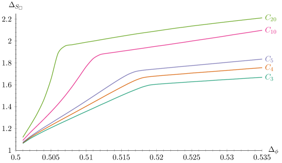
Fig.​ 1: Upper bound on the dimension of the first singlet scalar in the $\phi_{i}\times\phi_{j}$ OPE as a function of the dimension of $\phi$. Areas above the curves are excluded in the corresponding theories.

The high degree of similarity of Fig. 1 with the $O(N)$ bounds of [6] suggests that although we only require hypercubic symmetry, the bound on $\Delta_{S_{\square}}$ is saturated by the $O(N)$ solution. For $N=3$ we have explicitly checked that the bound obtained from the crossing equation (2.5) is exactly the same as that obtained from the $O(3)$ crossing equation. In the singlet sector, therefore, the $O(N)$ solution gets in the way and does not allow saturation of the bound with purely hypercubic theories, which lie somewhere in the allowed region.

We now move on to the $\text{V}_{\square}^{+}$ sector. A bound on the first scalar operator in that sector, called $V_{\square}$ here, is shown in Fig. 2.

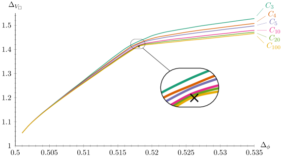
Fig.​ 2: Upper bound on the dimension of the first scalar operator in the $\text{V}^{+}_{\square}$ sector of the $\phi_{i}\times\phi_{j}$ OPE as a function of the dimension of $\phi$. Areas above the curves are excluded in the corresponding theories. The x-marker indicates the position of the decoupled Ising theory.

Perturbation theory gives us two hypercubic fixed points: one is fully interacting, while the other is obtained by taking $N$ decoupled Ising models [12]. In the latter case $V_{\square}$ has the scaling dimension of the $\epsilon$ operator in the Ising model, $\Delta_{\epsilon}\approx 1.4126$. While the putative theory that saturates the bound of Fig. 2 for small $N$ is unknown to us at this point, we can easily see that it is not the decoupled Ising one. Of course the latter is always in the allowed region, and in fact at large $N$ the bound gets closer to it.

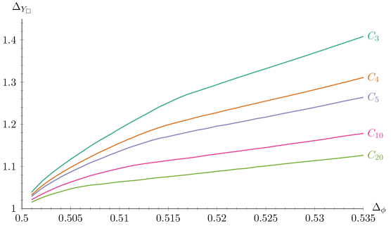
Fig.​ 3: Upper bound on the dimension of the first scalar operator in the $\text{Y}^{+}_{\square}$ sector of the $\phi_{i}\times\phi_{j}$ OPE as a function of the dimension of $\phi$. Areas above the curves are excluded in the corresponding theories.

We can also obtain bounds for the first scalar operator in the $\text{Y}_{\square}^{+}$ sector and the first vector operator in the $\text{A}_{\square}^{-}$ sector. These bounds are shown in Figs. 3 and 4, respectively. Unfortunately, they do not show any interesting features. In Fig. 4 the genaralized free theory line $2\Delta_{\phi}+1$ is of course in the allowed region of all bounds. Note that because the hypercubic symmetry is discrete we do not have a conserved current in the $\text{A}_{\square}^{-}$ sector.

Fig.​ 4: Upper bound on the dimension of the first vector operator in the $\text{A}^{-}_{\square}$ sector of the $\phi_{i}\times\phi_{j}$ OPE as a function of the dimension of $\phi$. Areas above the curves are excluded in the corresponding theories.

To recover the $O(N)$ solution the $V_{\square}$ and $Y_{\square}$ operators should have the same scaling dimension and combine to the lowest-dimension scalar traceless-symmetric operator of $O(N)$ with dimension $\Delta_{T_{\mathbin{\scalerel*{\bigcirc}{t}}}}$. That possibility should be allowed by our bounds in Figs. 2 and 3, i.e. $\Delta_{T_{\mathbin{\scalerel*{\bigcirc}{t}}}}$ should be in the allowed region of the corresponding bound in both Figs. 2 and 3. It is immediately verified based on the results of [6, 7] that this is indeed the case.

Some of our bounds can be compared with the $\varepsilon$ expansion using the three-loop result, see e.g. [28] or [17],

$$\Delta_{\phi}^{\varepsilon}=1-\tfrac{1}{2}\hskip 1.0pt\varepsilon+\frac{(N-1)(N+2)}{108N^{2}}\hskip 1.0pt\varepsilon^{2}+\frac{(N-1)(109N^{3}-222N^{2}+1728N-1696)}{11664N^{4}}\hskip 1.0pt\varepsilon^{3}+\text{O}(\varepsilon^{4})\,,$$ (3.1)

and the two-loop results of [17],

$$\begin{split}\Delta_{V_{\square}}^{\varepsilon}&=2-\frac{2(N+1)}{3N}\hskip 1.0pt\varepsilon+\frac{19N^{3}+131N^{2}-538N+424}{162N^{3}}\hskip 1.0pt\varepsilon^{2}+\text{O}(\varepsilon^{3})\,,\\ \Delta_{Y_{\square}}^{\varepsilon}&=2-\frac{3N-2}{3N}\hskip 1.0pt\varepsilon+\frac{3N^{3}-127N^{2}+530N-424}{162N^{3}}\hskip 1.0pt\varepsilon^{2}+\text{O}(\varepsilon^{3})\,.\end{split}$$ (3.2)

As an example, choosing $N=3$ and sending $\varepsilon\to 1$ neglecting $\text{O}(\varepsilon^{4})$ or $\text{O}(\varepsilon^{3})$ terms we find $\Delta_{\phi}^{\varepsilon=1}\approx 0.52$, $\Delta_{V_{\square}}^{\varepsilon=1}\approx 1.23$ and $\Delta_{Y_{\square}}^{\varepsilon=1}\approx 1.25$. These values are in the allowed regions of the corresponding bounds in Fig. 2 and Fig. 3. At large $N$ $\Delta_{\phi}^{\varepsilon=1}\approx 0.52$, $\Delta_{V_{\square}}^{\varepsilon=1}\approx 1.45$, and $\Delta_{Y_{\square}}^{\varepsilon=1}\approx 1.02$, so in that case $\Delta_{V_{\square}}^{\varepsilon=1}$ is in the excluded region of Fig. 2. Of course these $\varepsilon=1$ results should be taken with a grain of salt. Higher-order results for $\Delta_{V_{\square}}^{\varepsilon}$ and $\Delta_{Y_{\square}}^{\varepsilon}$ would allow proper resummations and the extraction of more meaningful results.

3.2 Analysis of the spectrum of the $C_{3}$ boundary solution

So far we have applied the standard numerical bootstrap logic for operator dimension bounds. Let us summarize it briefly and schematically here. First, we bring the crossing equation to the form

$$\sum_{\text{all sectors}}\!\!\!\!\lambda_{\mathcal{O}}^{2}\hskip 1.0pt\vec{V}_{\Delta,\hskip 1.0pt\ell}=-\vec{V}_{0,0}\,,$$ (3.3)

where in the right-hand side we have isolated the contribution of the identity operator, whose OPE coefficient has been normalized to unity. The vectors $\vec{V}$ stand for the various contributions in (2.5) for example. Now we take a linear functional $\vec{\alpha}$ of appropriate dimension and form the inner product with (3.3), i.e. we write

$$\sum_{\text{all sectors}}\!\!\!\!\lambda_{\mathcal{O}}^{2}\,\vec{\alpha}\cdot\vec{V}_{\Delta,\hskip 1.0pt\ell}=-\vec{\alpha}\cdot\vec{V}_{0,0}\,.$$ (3.4)

At this point we make an assumption on the spectrum and we scan over the space of linear functionals $\vec{\alpha}$ demanding

$$\vec{\alpha}\cdot\vec{V}_{0,0}=1\,,\qquad\vec{\alpha}\cdot\vec{V}_{\Delta,\hskip 1.0pt\ell}\geq 0\,,\text{ for all allowed }\Delta,\hskip 1.0pt\ell.$$ (3.5)

If we manage to find such a functional, then (3.4) leads to a contradiction and so the assumption we made on the spectrum is not consistent with unitarity (i.e. with assuming that all $\lambda_{\mathcal{O}}$’s are real).

Right at the boundary of the allowed region knowledge of the functional is enough to give us information about the spectrum of the actual solution to crossing symmetry there [29, 30]. This is because when we cross the bound we go from having a functional to not having one, which means that right on the boundary of the allowed and the disallowed region (on the disallowed side) the action of the associated extremal functional should saturate the inequalities in (3.5) and give zero on $\vec{V}_{\Delta,\hskip 1.0pt\ell}$ for all physical operators in the spectrum. In other words, right on the bound (on the disallowed side) the left-hand side of (3.4) is zero because all contributions (at discrete $\Delta$’s for allowed $\ell$’s) are zero. Note that the right-hand side of (3.4) is equal to $-1$ due to (3.5). The functional we obtain is thus truly extremal when for generic $\Delta,\ell$ outside the spectrum $\vec{\alpha}\cdot\vec{V}_{\Delta,\hskip 1.0pt\ell}/\vec{\alpha}\cdot\vec{V}_{0,0}\to\infty$.

Our results below are extracted by plotting the logarithm of the action of the functional on the convolved conformal blocks and looking at the positions of the dips in those plots. These give us the scaling dimensions of operators that solve crossing at the bound.

Let us first obtain the functional along the bound of Fig. 1. From the spectrum in the $\text{V}_{\square}^{+}$, $\text{Y}_{\square}^{+}$ and $\text{A}_{\square}^{-}$ sectors we can verify that our $\Delta_{S_{\square}}$ bound is saturated by the $O(N)$ solution. Indeed, operators in the $\text{V}_{\square}^{+}$ and $\text{Y}_{\square}^{+}$ sectors have the same scaling dimension, and the first operator in the $\text{A}_{\square}^{-}$ sector has dimension exactly equal to two.

We will now perform an analysis of the spectrum along the $C_{3}$ bound using the functional obtained from Fig. 2. We will refer to the spectrum at the kink as the $C_{3}^{b}$ solution. Note that we have obtained the bound of Fig. 2 with a vertical tolerance of $10^{-6}$ for the spectrum analysis that follows. We would like to mention that the results reported in the remainder of this section do not change by making the numerics more demanding. We have checked this by running with $\texttt{nmax}=11$, $\texttt{mmax}=8$, $\texttt{kmax}=36$, $\texttt{cutoff}=10^{-12}$ in PyCFTBoot, and including spins up to $\ell_{\text{max}}=32$.

First, we look at the dimension of $S_{\square}^{b}$ in the $C_{3}^{b}$ solution in Fig. 5. Our result is that the $C_{3}^{b}$ solution at the kink, occurring at $\Delta_{\phi}\approx 0.518$, has much lower $\Delta_{S_{\square}^{b}}$ than $\Delta_{S_{\mathbin{\scalerel*{\bigcirc}{t}}}}$ at the $O(3)$ fixed point. Indeed, we find $\Delta_{S_{\square}^{b}}\approx 1.329$, while [8] gives $\Delta_{S_{\mathbin{\scalerel*{\bigcirc}{t}}}}\approx 1.5957$. This suggests that the $C_{3}^{b}$ solution does not correspond to the $C_{3}^{\varepsilon}$ theory found with the $\varepsilon$ expansion, where the scaling dimensions $\Delta_{S_{\square}^{\varepsilon}}$ and $\Delta_{S_{\mathbin{\scalerel*{\bigcirc}{t}}}}$ at $C_{3}^{\varepsilon}$ and $O(3)$, respectively, are calculated to be nearly degenerate [18, 19, 9].

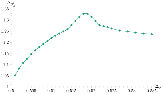
Fig.​ 5: The dimension of $S_{\square}^{b}$ at the $C_{3}^{b}$ solution, i.e. assuming that $\Delta_{V_{\square}}$ is equal to the bound of Fig. 2. The markers indicate the points at which we have computed the spectrum.

We would also like to note here that we now have a further indication that the bound in Fig. 2 is not saturated by the decoupled Ising theory. Indeed, if that were the case then the dimension of $S_{\square}^{b}$ should be equal to that of the $\epsilon$ operator in the Ising model, which is clearly not the case based on Fig. 5.

We can also fix $\Delta_{\phi}$ to its value at the kink, $\Delta_{\phi}=0.518$, and obtain a bound on $\Delta_{V_{\square}}$ by imposing a gap on $\Delta_{S_{\square}}$ in the allowed region of Fig. 1. That is, instead of allowing $\Delta_{S_{\square}}$ above the unitarity bound, we allow it only above the value in the figure. This bound is shown in Fig. 6.

We may also obtain the dimension of the second scalar singlet in the $\phi_{i}\times\phi_{j}$ OPE, called $S_{\square}^{\prime\hskip 0.5ptb}$ here. If the scaling dimension of this operator were less than three, then $C_{3}^{b}$ would be a tricritical solution (two relevant scalar singlets). From Fig. 7 we see that $\Delta_{S_{\square}^{\prime\hskip 0.5ptb}}>3$ around $\Delta_{\phi}=0.518$, and so $C_{3}^{b}$ is a critical solution (one relevant scalar singlet).

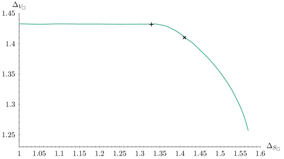
Fig.​ 6: Upper bound on $\Delta_{V_{\square}}$ as a function of the gap on $\Delta_{S_{\square}}$ assuming $\Delta_{\phi}=0.518$ for $N=3$. The x- and +-markers indicate the position of the decoupled Ising and the $C_{3}^{b}$ solution, respectively.

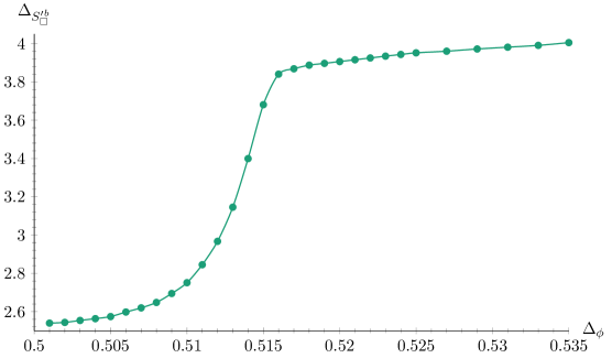
Fig.​ 7: The dimension of $S_{\square}^{\prime\hskip 0.5ptb}$ at the $C_{3}^{b}$ solution, i.e. assuming that $\Delta_{V_{\square}}$ is equal to the bound of Fig. 2. The markers indicate the points at which we have computed the spectrum.

3.3 Discussion

Our results may have implications for the theory of structural phase transitions. It was suggested a long time ago [18] that critical exponents of the $C_{3}^{\varepsilon}$ theory should be compared to experiment, for example the structural phase transition of $\text{SrTiO}_{3}$ (strontium titanate) [33, 34, 35, 36, 37] where the lattice structure undergoes a transition from cubic to tetragonal at a critical temperature $T_{c}\approx 100\text{ K}$. Crystals of the type ABX₃ are called perovskites. X is usually oxygen. The undistorted (high-temperature) phase has A on the corners of a cube, B at the base center, and X₃ at the face centers; see Fig. 8.

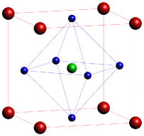
Fig.​ 8: The perovskite structure ABX₃. A is red, B is green, and X₃ is blue.

In these systems, and in the context of the Landau theory of phase transitions, a term preserving cubic symmetry is allowed in the expansion of the free energy, and so its effects need to be taken into consideration [38, sec. I.4.2]. A transition to a distorted phase occurs due to rotations of the X₃ octahedra around a four-fold axis of the cube as the temperature is lowered below a critical value. The phase transition is continuous (second order), in the sense that the rotation of the octahedra is continuous. The crystal structure above and below the transition temperature is depicted in Fig. 9 in a top-down view.

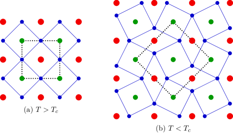
Fig.​ 9: The crystal structure in a top-down view above (a) and below (b) the critical transition temperature $T_{c}\approx 100\text{ K}$. The unit cell is highlighted by the dotted line.

In the third direction two adjacent octahedra rotate in opposite directions and so the unit cell is enlarged by a factor of 2 in that direction. Taking everything into account the unit cell of the distorted phase is enlarged by $\sqrt{2}\times\sqrt{2}\times 2$ relative to the undistorted phase, and so it belongs to the tetragonal crystal system. The symmetry of the undistorted phase is given by the group $O_{h}$ (which is the same as what we call $C_{3}$), while that of the distorted phase is given by the 16-element group $D_{4h}$. A review on structural phase transitions is [38, 39], while some information can also be found in [40, Chapter XIV].

As we already mentioned, the $\varepsilon$ expansion gives $\Delta_{S_{\square}^{\varepsilon}}$ very close to $\Delta_{S_{\mathbin{\scalerel*{\bigcirc}{t}}}}$ [18, 19, 9], which was already noticed in [18] as a possible disagreement with experiment. It was later suggested that residual strains in the crystals used in the experiments may be responsible for a crossover to Ising-like behavior [41]. The Ising critical exponents match the experimental results very well, thus offering a way out of the apparent incompatibility between the $\varepsilon$ expansion results and the experiments. The suggestion that systematic strains induce an Ising-like behavior was investigated in subsequent experiments [42]. To our knowledge critical exponents in strain-free crystals have not been reported, although such results are mentioned in [37] (presumably pertaining to [43]) to be close to those obtained in crystals with strains. In light of our results it would be very interesting to revisit these experiments in order to see if our $C_{3}^{b}$ solution corresponds to the theory describing structural phase transitions of strain-free perovskites.

Our results also imply that the $C_{3}^{b}$ solution is not relevant for cubic magnets, whose critical exponents have been measured and found close to those predicted by the $O(3)$ model and the $C_{3}^{\varepsilon}$ theory [9]. This is despite the fact that the $C_{3}^{b}$ solution has only one relevant scalar singlet, as we deduce from Fig. 7. We do not know if the cubic deformation is relevant in the $O(3)$ theory. Note that in the $O(N)$ model the cubic deformation is drawn from a traceless-symmetric scalar operator with four $O(N)$ indices, $\mathcal{O}_{ijkl}$ [9]. In the $\varepsilon$ expansion it is known that, when it exists, the stable fixed point is unique [20]. If the $C_{3}^{b}$ solution were to correspond to the $C_{3}^{\varepsilon}$ theory, then the non-perturbative situation would contradict that intuition. On the one hand cubic magnets would be described by the $O(3)$ theory at criticality according to the experimental results. This would mean that at the $O(3)$ fixed point the cubic deformation is not relevant. On the other hand the bootstrap would be showing that $C_{3}^{b}$ has just one relevant operator and so it would correspond to a stable fixed point. Despite that, cubic magnets at criticality would not be in this universality class.

We would then be forced to conclude that neither the $C_{3}^{b}$ or $O(3)$ fixed point has a second relevant operator (assuming that the critical exponents of cubic magnets have been measured correctly). Besides the possibility that both fixed points are stable, it could also be that the $O(3)$ model has an exactly marginal operator. A Monte Carlo study of the cubic deformation at the $O(3)$ fixed point was performed in [13]. Their results for the anomalous dimension of the cubic deformation are consistent with the value zero. If zero were indeed the correct answer, this would obviously imply that the cubic deformation is exactly marginal at the $O(3)$ fixed point. The necessary condition is that a traceless-symmetric scalar operator $\mathcal{O}_{ijkl}$ of the $O(3)$ theory has dimension exactly equal to three. To our knowledge this has not been excluded in the literature, but without a principle that would fix the dimension of $\mathcal{O}_{ijkl}$ to three it seems unlikely.

3.4 Central charge bounds

Without any assumptions we can bound the central charge $C_{\square}$ as a function of $\Delta_{\phi}$. Here we present lower bounds on the ratio $C_{\square}/C_{\text{free}}$, where $C_{\text{free}}=\frac{3}{2}N$. We remind the reader that $C$ appears in the coefficient of the two-point function of the stress-energy tensor, which in $d$ dimensions is constrained by conformal invariance to be of the form

$$\langle T_{\mu\nu}(x)\hskip 0.5ptT_{\rho\sigma}(0)\rangle=C\frac{1}{S_{d}^{\hskip 0.5pt2}}\frac{1}{(x^{2})^{d}}\hskip 1.0pt\mathcal{I}_{\mu\nu\rho\sigma}(x)\,,$$ (3.6)

where $S_{d}=2\pi^{\frac{1}{2}d}/\Gamma(\frac{1}{2}d)$ and

$$\qquad\mathcal{I}_{\mu\nu\rho\sigma}=\tfrac{1}{2}(I_{\mu\rho}\hskip 1.0ptI_{\nu\sigma}+I_{\mu\sigma}\hskip 1.0ptI_{\nu\rho})-\frac{1}{d}\hskip 1.0pt\eta_{\mu\nu}\eta_{\rho\sigma}\,,\qquad I_{\mu\nu}=\eta_{\mu\nu}-\frac{2}{x^{2}}\hskip 1.0ptx_{\mu}x_{\nu}\,.$$ (3.7)

In these conventions a free scalar’s contribution to the central charge is equal to $d/(d-1)$.

Without any assumptions the bounds are shown in Fig. 10. They are essentially identical to the ones obtained for the $O(N)$ models [6].

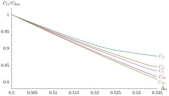
Fig.​ 10: Lower bound on the central charge as a function of the dimension of $\phi$. Areas below the curves are excluded in the corresponding theories.

For $C_{3}$ we may assume, as we have before, that $\Delta_{V_{\square}}$ saturates the bound of Fig. 2 (obtained with a vertical tolerance of $10^{-6}$). The value of $C_{\square}^{b}$ is then shown in Fig. 11. Much like in the $O(N)$ and Ising models there is a minimum. As we see it is rather wide and is attained slightly to the left of $\Delta_{\phi}=0.52$. Based on Fig. 11 we may conclude that the $C_{3}^{b}$ solution has a central charge slightly higher than the $O(3)$ value [6], namely $C_{\square}^{b}\approx 0.947\times 3\times\frac{3}{2}$, while $C_{\mathbin{\scalerel*{\bigcirc}{t}}}\approx 0.944\times 3\times\frac{3}{2}$.

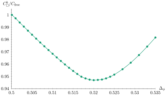
Fig.​ 11: Value of the central charge of the $C_{3}^{b}$ solution as a function of the dimension of $\phi$.

4 Hypertetrahedral symmetry

Hypertetrahedral symmetry may be implemented by considering $N+1$ vectors $e_{i}{\!}^{\alpha}$, $\alpha=1,2,\dots,N+1$, forming the vertices of an $N$-dimensional hypertetrahedron, satisfying

$${\sum_{\alpha}}\,e_{i}{\!}^{\alpha}=0,\,\qquad{\sum_{\alpha}}\,e_{i}{\!}^{\alpha}e_{j}{\!}^{\alpha}=\delta_{ij}\,,\qquad e_{i}{\!}^{\alpha}e_{i}{\!}^{\beta}=\delta^{\alpha\beta}-\frac{1}{N+1}\equiv P^{\alpha\beta}\,.$$ (4.1)

In this case the symmetry group is $T_{N}=\mathcal{S}_{N+1}$, and we can borrow some results from the literature. Crucial representation theory was worked out in [44, 45]. In [46] the four-point function of the field $\phi^{\alpha}=e_{i}{\!}^{\alpha}\phi_{i}$ was given. Using results of [47, 48] one can indeed write, in the $12\rightarrow 34$ channel,

$$\begin{split}x_{12}^{2\Delta_{\phi}}x_{34}^{2\Delta_{\phi}}\langle\phi^{\alpha}(x_{1})\phi^{\beta}(x_{2})\phi^{\gamma}(x_{3})\phi^{\delta}(x_{4})\rangle&=\sum_{\text{S}^{+}_{\triangle}}\lambda_{\mathcal{O}}^{2}\hskip 1.0ptP^{\alpha\beta}P^{\gamma\delta}g_{\Delta,\hskip 1.0pt\ell}(u,v)+\sum_{\text{V}^{+}_{\triangle}}\lambda_{\mathcal{O}}^{2}\hskip 1.0ptQ^{\alpha\beta\gamma\delta}\hskip 1.0ptg_{\Delta,\hskip 1.0pt\ell}(u,v)\\ &\quad+\sum_{\text{Y}^{+}_{\triangle}}\lambda_{\mathcal{O}}^{2}\hskip 1.0ptR^{\alpha\beta\gamma\delta}g_{\Delta,\hskip 1.0pt\ell}(u,v)+\sum_{\text{A}^{-}_{\triangle}}\lambda_{\mathcal{O}}^{2}\hskip 1.0ptS^{\alpha\beta\gamma\delta}g_{\Delta,\hskip 1.0pt\ell}(u,v)\,,\end{split}$$ (4.2)

where

$$\begin{split}Q^{\alpha\beta\gamma\delta}&=\Big{(}\delta^{\alpha\beta}-\frac{2}{N+1}\Big{)}\Big{(}\delta^{\gamma\delta}-\frac{2}{N+1}\Big{)}\Big{(}\delta^{\alpha\gamma}+\delta^{\alpha\delta}+\delta^{\beta\gamma}+\delta^{\beta\delta}-\frac{4}{N+1}\Big{)}\,,\\ R^{\alpha\beta\gamma\delta}&=\delta^{\alpha\neq\beta}\delta^{\gamma\neq\delta}\Big{(}\delta^{\alpha\gamma}\delta^{\beta\delta}+\delta^{\alpha\delta}\delta^{\beta\gamma}-\frac{1}{N-1}(\delta^{\alpha\gamma}+\delta^{\alpha\delta}+\delta^{\beta\gamma}+\delta^{\beta\delta})+\frac{2}{N(N-1)}\Big{)}\,,\\ S^{\alpha\beta\gamma\delta}&=\delta^{\alpha\gamma}\delta^{\beta\delta}-\delta^{\alpha\delta}\delta^{\beta\gamma}-\frac{1}{N+1}(\delta^{\alpha\gamma}-\delta^{\alpha\delta}-\delta^{\beta\gamma}+\delta^{\beta\delta})=P^{\alpha\gamma}P^{\beta\delta}-P^{\alpha\delta}P^{\beta\gamma}\,.\end{split}$$ (4.3)

It is easy to show that

$$Q^{\alpha\beta\gamma\delta}=4\hskip 1.0pt\Big{(}P^{\alpha\beta}P^{\alpha\gamma}P^{\gamma\delta}-\frac{1}{N+1}(P^{\alpha\beta}P^{\alpha\delta}+P^{\beta\gamma}P^{\gamma\delta})+\frac{1}{(N+1)^{2}}P^{\beta\delta}\Big{)}\,,$$ (4.4)

and, using $\delta^{a\neq\beta}=1-\delta^{\alpha\beta}$, that

$$\begin{split}R^{\alpha\beta\gamma\delta}&=-\frac{N+1}{2\hskip 0.5pt(N-1)}\hskip 1.0ptQ^{\alpha\beta\gamma\delta}+P^{\alpha\gamma}P^{\beta\delta}+P^{\alpha\delta}P^{\beta\gamma}-\frac{2}{N}P^{\alpha\beta}P^{\gamma\delta}\,.\end{split}$$ (4.5)

With (4.4) and (4.5) the crossing equation that arises from (4.2) can be easily worked out. We find

$$\sum_{\text{S}_{\triangle}^{+}}\lambda_{\mathcal{O}}^{2}\begin{pmatrix}0\\ F^{-}_{\Delta,\hskip 1.0pt\ell}\\ F^{+}_{\Delta,\hskip 1.0pt\ell}\\ 0\end{pmatrix}+\sum_{\text{V}_{\triangle}^{+}}\lambda_{\mathcal{O}}^{2}\begin{pmatrix}0\\ 0\\ -\frac{4}{N+1}F^{+}_{\Delta,\hskip 1.0pt\ell}\\ F^{-}_{\Delta,\hskip 1.0pt\ell}\end{pmatrix}+\sum_{\text{Y}_{\triangle}^{+}}\!\lambda_{\mathcal{O}}^{2}\begin{pmatrix}F^{-}_{\Delta,\hskip 1.0pt\ell}\\ \frac{2\hskip 0.5pt(N-1)}{N}\hskip 1.0ptF^{-}_{\Delta,\hskip 1.0pt\ell}\\ -\tfrac{(N+1)(N-2)}{N(N-1)}F^{+}_{\Delta,\hskip 1.0pt\ell}\\ -\frac{N+1}{2\hskip 0.5pt(N-1)}F^{-}_{\Delta,\hskip 1.0pt\ell}\end{pmatrix}+\sum_{\text{A}_{\triangle}^{-}}\lambda_{\mathcal{O}}^{2}\begin{pmatrix}F^{-}_{\Delta,\hskip 1.0pt\ell}\\ 0\\ F^{+}_{\Delta,\hskip 1.0pt\ell}\\ 0\end{pmatrix}=\begin{pmatrix}0\\ 0\\ 0\\ 0\end{pmatrix}.$$ (4.6)

This crossing equation is equivalent to the one that recently appeared in [21].

Using the primitive invariant tensor $d_{ijkl}$ of [12] for the hypertetrahedral case and the relation

$$d_{ijmn}d_{mnkl}=\frac{N(N-2)}{(N+1)(N+2)^{2}}\Big{(}\delta_{ik}\delta_{jl}+\delta_{il}\delta_{jk}-\frac{2}{N}\delta_{ij}\delta_{kl}\Big{)}+\frac{N^{2}-3N-2}{(N+1)(N+2)}\hskip 1.0ptd_{ijkl}\,,$$ (4.7)

we can find the projectors

$$\begin{split}P_{ijkl}^{(1)}&=\frac{1}{N}\delta_{ij}\delta_{kl}\,,\\ P_{ijkl}^{(2)}&=\frac{N+1}{N-1}\hskip 1.0ptd_{ijkl}+\frac{N}{(N-1)(N+2)}\Big{(}\delta_{ik}\delta_{jl}+\delta_{il}\delta_{jk}-\frac{2}{N}\delta_{ij}\delta_{kl}\Big{)}\,,\\ P_{ijkl}^{(3)}&=-\frac{N+1}{N-1}\hskip 1.0ptd_{ijkl}+\frac{(N-2)(N+1)}{2(N-1)(N+2)}\Big{(}\delta_{ik}\delta_{jl}+\delta_{il}\delta_{jk}-\frac{2}{N}\delta_{ij}\delta_{kl}\Big{)}\,,\\ P_{ijkl}^{(4)}&=-\tfrac{1}{2}(\delta_{ik}\delta_{jl}-\delta_{il}\delta_{jk})\,.\end{split}$$ (4.8)

Just like in the hypercubic case these satisfy (2.7).

It is straightforward to verify that for $N=3$ (4.6) and (2.5) are equivalent, with $\text{V}^{+}_{\triangle}\leftrightarrow\text{Y}^{+}_{\square}$ and $\text{Y}^{+}_{\triangle}\leftrightarrow\text{V}^{+}_{\square}$ . This equivalence is a consequence of the fact that for $N=3$ the vertices of the tetrahedron also form diagonals of the cube [11]. For other $N$ the hypertetrahedral group is not a subgroup of the hypercubic group. We should note here that our symmetry group is really $\mathcal{S}_{N+1}\times\mathbb{Z}_{2}$. The $\mathbb{Z}_{2}$ gives a minus sign to all fields, and it can be broken if we assume that $\phi^{\gamma}$ appears in the OPE $\phi^{\alpha}\times\phi^{\beta}$. In this work we do not make this assumption.

Let us now mention some results that the $\varepsilon$ expansion gives for hypertetrahedral theories [12]. For generic $N$ there are two hypertetrahedral fixed points with

$$\begin{split}\Delta_{\phi}^{\!T^{(1)}_{N}}&=\tfrac{1}{2}(d-2)+\frac{(N+1)(N+7)}{108\,(N+3)^{2}}\varepsilon^{2}+\frac{(N+1)(109N^{3}+969N^{2}+5463N+7411)}{11664(N+3)^{4}}\,\varepsilon^{3}\,,\\ \Delta_{\phi}^{\!T^{(2)}_{N}}&=\tfrac{1}{2}(d-2)+\frac{(N-1)(N-2)(N^{2}-6N+11)}{108\,(N^{2}-5N+8)^{2}}\,\varepsilon^{2}\\ &+\frac{(N-1)(N-2)(109N^{6}-1752N^{5}+12336N^{4}-48804N^{3}+114807N^{2}-151944N+88208)}{11664(N^{2}-5N+8)^{4}}\,\varepsilon^{3}\,.\end{split}$$ (4.9)

These fixed points do not exist for all $N$. In the framework of the $\varepsilon$ expansion one can see that the hypertetrahedral fixed points collide and disappear into the complex plane at some $N_{-}$, and again reappear at some $N_{+}$. These are given by [12]

$$N_{\pm}=5+6\,\varepsilon+\tfrac{281}{32}\,\varepsilon^{2}-\tfrac{61}{8}\,\zeta_{3}\,\varepsilon^{2}\pm\sqrt{24\,\varepsilon+\tfrac{289}{4}\,\varepsilon^{2}-30\,\zeta_{3}\,\varepsilon^{2}}\,,$$ (4.10)

where $\zeta_{3}$ is Apéry’s constant. For $N_{-}<N<N_{+}$ there are no hypertetrahedral fixed points. If we brazenly plug in $\varepsilon=1$ to (4.10) we find

$$N_{\pm}\approx 10.62\pm 7.76\,.$$ (4.11)

5 Bounds in hypertetrahedral theories

In the singlet sector the bound on $\Delta_{S_{\triangle}}$ is again saturated by the $O(N)$ solution. A bound on the dimension of the first scalar operator in the $\text{V}^{+}_{\triangle}$ sector is shown in Fig. 12.

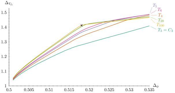
Fig.​ 12: Upper bound on the dimension of the first scalar operator in the $\text{V}^{+}_{\triangle}$ sector of the $\phi^{\alpha}\times\phi^{\beta}$ OPE as a function of the dimension of $\phi$. Areas above the curves are excluded in the corresponding theories. The x-marker indicates the position of the decoupled Ising theory.

As we see, for low values of $N$ there is no kink in the bounds. The kink develops as $N$ increases; this is consistent with the absence of CFTs with hypertetrahedral symmetry for low values of $N$ as expected from (4.11). We also see that at large $N$ the decoupled Ising theory is in the allowed region and in fact saturates the bound.

Although for $N=3$ there is no kink in the bound of Fig. 12, a kink appears in the $\text{Y}_{\triangle}^{+}$ sector as in Fig. 13. Indeed, for $N=3$ we see a kink in the dimension of $Y_{\triangle}\equiv V_{\square}$. This is the same as the kink in the $C_{3}$ curve of Fig. 2, and so its interpretation as a CFT is questionable. No kink is seen for other values of $N$, however, consistently with our expectations from the $\varepsilon$ expansion.

Although a precise determination of $N_{\pm}$ with the bootstrap of a single correlator is perhaps not feasible, we expect $N_{-}\lesssim 4$ and $N_{+}\lesssim 15$ based on the presence of a kink in the bound of $\Delta_{V_{\triangle}}$. We have looked at the spectrum of the solution that saturates the bounds of Fig. 12, but we have not been able to identify a feature that can serve as a conclusive indicator of the existence of a CFT. It would be interesting to study this important problem in a mixed-correlator setting.

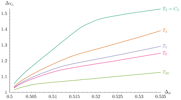
Fig.​ 13: Upper bound on the dimension of the first scalar operator in the $\text{Y}^{+}_{\triangle}$ sector of the $\phi^{\alpha}\times\phi^{\beta}$ OPE as a function of the dimension of $\phi$. Areas above the curves are excluded in the corresponding theories.

6 Conclusion

In this paper we studied hypercubic and hypertetrahedral theories in $d=3$ with the non-perturbative numerical conformal bootstrap. We focused mainly on the $N=3$ cubic theory due to its importance for phase transitions of cubic magnets and perovskites. We found that the bound of the first scalar operator in the $\text{V}_{\square}^{+}$ sector is saturated by a kink solution, called $C_{3}^{b}$, with properties that cannot be reconciled with the $\varepsilon$ expansion.

There are (at least) three possibilities for the fate of $C_{3}^{b}$ (and $C_{N}^{b}$):

1. it corresponds to a hypercubic CFT that is inaccessible with the $\varepsilon$ expansion,

2. it corresponds to the hypercubic CFT found with the $\varepsilon$ expansion,

3. it does not correspond to an actual CFT.

Perhaps the most conservative possibility is the last one. The presence of the kink would then be an artifact of the numerics. In any case, without independent arguments at our disposal we cannot convincingly settle on the correct interpretation of $C_{N}^{b}$.

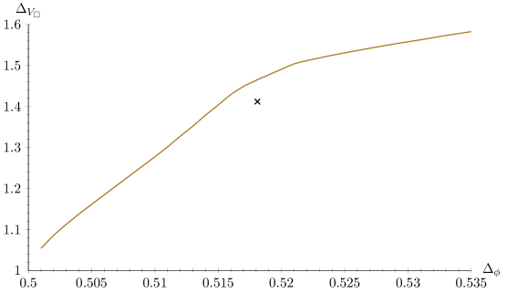
Fig.​ 14: Upper bound on the dimension of the first $\text{V}_{\square}^{+}$ scalar operator in the $\phi_{i}\times\phi_{j}$ OPE as a function of the dimension of $\phi$ for $N=2$. The area above the curve is excluded. The x-marker indicates the position of the decoupled Ising theory.

According to the $\varepsilon$ expansion for $N=2$ there is no fully-interacting CFT other than the $O(2)$ model in $d=4-\varepsilon$ [12]. The only solution with “cubic symmetry” for $N=2$ is the decoupled Ising model. We would thus expect the $N=2$ bound on $\Delta_{V_{\square}}$ to be saturated at the Ising point. This is, however, not what we find, as we see in Fig. 14. The bound is in fact weaker than the $C_{3}$ bound of Fig. 2. The (smooth) kink observed suggests that there may be a CFT not seen by the $\varepsilon$ expansion, or that a CFT with higher symmetry gets in the way. It could also be an artifact of the numerics and correspond to no actual CFT.

Let us close by reminding the reader that when $N\to\infty$ the hypercubic theory should go the constrained Ising model [49, 50, 51], in which the first scalar singlet has scaling dimension $3-\Delta_{\epsilon}\approx 1.5874$. This is a non-perturbative result. We have checked that this is not what happens for $C_{\infty}^{b}$, i.e. for the solution obtained at the kink of the bound on the dimension of $V_{\square}$ at large $N$. However, in the $\Delta_{V_{\square}}\text{-}\Delta_{\phi}$ slice of parameter space there are two CFTs at the same exact position for $N\to\infty$. One is the decoupled Ising theory, and the other is the constrained Ising one. In the former the lowest-dimension singlet scalar has dimension $\Delta_{\epsilon}\approx 1.4126$, while in the latter it has dimension $3-\Delta_{\epsilon}$. Therefore, the interpretation of the spectrum of the $C_{\infty}^{b}$ solution in that case, solely derived from the solution at the kink in the $\Delta_{V_{\square}}\text{-}\Delta_{\phi}$ slice, is unclear. It is plausible that in order to derive meaningful results one needs to use information from other sectors of operators, specifically those in which the two CFTs do not have spectra of operators with the same scaling dimensions.

Acknowledgments

I would like to thank Stefanos R. Kousvos and Theodore N. Tomaras for collaboration in the initial stages of this project, and for many helpful discussions. I also thank Connor Behan for help with PyCFTBoot, and Kostas Siampos and Alessandro Vichi for very useful discussions and comments. Finally, I am grateful to Amnon Aharony, Hugh Osborn, David Poland, Slava Rychkov, and Alessandro Vichi for comments on the manuscript. The numerical computations in this paper were run on the LXPLUS cluster at CERN.

Appendix A. An analysis of $C_{3}^{b}$ in $d=3.8$

In this appendix we study the $C_{3}^{b}$ solution in fractional spacetime dimension, namely $d=3.8$. We expect our analysis not to be invalidated by the fact that in such fractional dimensions unitarity is not expected to be present [52]. For the Ising model a similar analysis was performed in [53]. Our aim is to explore the properties of the $C_{3}^{b}$ solution, and compare with the $\varepsilon$ expansion at $\varepsilon=0.2$, a value we expect is low enough for perturbative results to be more trustworthy than in the $\varepsilon=1$ case. Again, $\Delta_{S_{\square}^{\varepsilon}}$ and $\Delta_{S_{\mathbin{\scalerel*{\bigcirc}{t}}}}$ are expected to be very close according to the $\varepsilon$ expansion. For the plots of this appendix we use $\texttt{nmax}=9$, $\texttt{mmax}=6$, $\texttt{kmax}=40$, $\texttt{cutoff}=10^{-15}$ in PyCFTBoot, and the same options and parameters as before for SDPB. We find the bounds with a vertical tolerance of $10^{-6}$.

First, we obtain a bound on the first singlet scalar in the $O(3)$ model, using the $O(N)$ crossing equation directly [6]. The bound is shown in Fig. 15, and it displays a strong kink around $\Delta_{\phi}=0.9005$. If the $O(3)$ model lives on the kink, then $\Delta_{S_{\mathbin{\scalerel*{\bigcirc}{t}}}}\approx 1.8969$.

The bound on the scaling dimension of $V_{\square}$ is shown in Fig. 16. There is again a very sharp kink. On the bound at $\Delta_{\phi}\approx 0.90045$ we have $\Delta_{V_{\square}}\approx 1.8710$. At this point it is not easy to tell if the kink is actually saturated by the decoupled Ising theory, for in the latter case the dimension of $V_{\square}$ would be equal to the dimension of the $\epsilon$ operator in the Ising model, which in $d=3.8$ is very close to 1.87. This can be seen both with the $\varepsilon$ expansion [54], and by looking at the relevant kink in [53]. To resolve this we look at the spectrum.

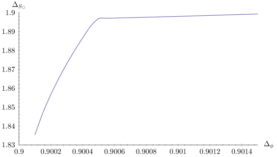
Fig.​ 15: Upper bound on the dimension of the first singlet scalar in the $\phi_{i}\times\phi_{j}$ OPE as a function of the dimension of $\phi$ in the $O(3)$ model in $d=3.8$.

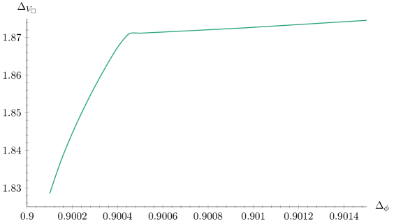
Fig.​ 16: Upper bound on the dimension of the first $\text{V}_{\square}^{+}$ scalar operator in the $\phi_{i}\times\phi_{j}$ OPE as a function of the dimension of $\phi$ in the $C_{3}$ theory in $d=3.8$.

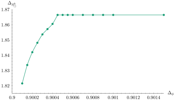
Fig.​ 17: The dimension of $S_{\square}^{b}$ at the $C_{3}^{b}$ solution in $d=3.8$, i.e. assuming that $\Delta_{V_{\square}}$ is equal to the bound of Fig. 16. The markers indicate the points at which we have computed the spectrum.

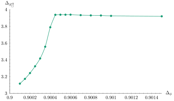
Fig.​ 18: The dimension of $S_{\square}^{\prime\hskip 0.5ptb}$ at the $C_{3}^{b}$ solution in $d=3.8$, i.e. assuming that $\Delta_{V_{\square}}$ is equal to the bound of Fig. 16. The markers indicate the points at which we have computed the spectrum.

The scaling dimensions of the first and second scalar singlet of $C_{3}^{b}$ are shown in Figs. 17 and 18, respectively. At the kink we have $\Delta_{S_{\square}^{b}}\approx 1.8665$. Although close to $\Delta_{V_{\square}^{b}}\approx 1.8710$, the two dimensions are different which gives us confidence that we are not in the decoupled Ising theory. For the second scalar singlet we have $\Delta_{S_{\square}^{\prime\hskip 0.5ptb}}>3.8$, which means that the $C_{3}^{b}$ solution is critical in $d=3.8$.

Finally we can compare with $\Delta_{S_{\mathbin{\scalerel*{\bigcirc}{t}}}}\approx 1.8969$ in $d=3.8$. For $\varepsilon=0.2$ we have $\Delta_{S_{\mathbin{\scalerel*{\bigcirc}{t}}}}-\Delta_{S_{\square}^{b}}\approx 0.03$. The results for $\Delta_{S_{\mathbin{\scalerel*{\bigcirc}{t}}}}$ and $\Delta_{S_{\square}^{b}}$ are significantly closer compared to the $\varepsilon=1$ case considered in the main text, where $\Delta_{S_{\mathbin{\scalerel*{\bigcirc}{t}}}}-\Delta_{S_{\square}^{b}}\approx 0.2667$. Nevertheless, we would expect a much smaller $\Delta_{S_{\mathbin{\scalerel*{\bigcirc}{t}}}}-\Delta_{S_{\square}^{b}}$ if the $C_{3}^{b}$ solution at the kink were to become the $C_{3}^{\varepsilon}$ CFT found with the $\varepsilon$ expansion at $\varepsilon=0.2$. Using the five-loop results of [54, 28] we find, using a simple Padé[3, 4] approximant, $\Delta_{S_{\mathbin{\scalerel*{\bigcirc}{t}}}}-\Delta_{S_{\square}^{\varepsilon=0.2}}\approx-2.5\times 10^{-4}$. The negative sign here seems to be at odds with the bootstrap results, but, given the smallness of $|\Delta_{S_{\mathbin{\scalerel*{\bigcirc}{t}}}}-\Delta_{S_{\square}^{\varepsilon=0.2}}|$, we expect this issue to be resolved by considering higher-order corrections and/or more robust resummation techniques. With the same Padé[3, 4] approximant we find $\Delta_{S_{\mathbin{\scalerel*{\bigcirc}{t}}}}-\Delta_{S_{\square}^{\varepsilon=1}}\approx 0.01$. At $\varepsilon=1$ more advanced resummation techniques give $\Delta_{S_{\mathbin{\scalerel*{\bigcirc}{t}}}}-\Delta_{S_{\square}^{\varepsilon=1}}\approx 6\times 10^{-4}$ [19, 9]. From this analysis we may then conclude that it is not likely that the $C_{3}^{b}$ solution at the kink is related to the $C_{3}^{\varepsilon}$ cubic CFT. However, given that there is a sharp kink in Fig. 16 we may speculate that the $C_{3}^{b}$ solution is in fact accessible with the $\varepsilon$ expansion. We hope to return to these issues in the future.

References

- [1] R. Rattazzi, V. S. Rychkov, E. Tonni & A. Vichi, “Bounding scalar operator dimensions in 4D CFT”, JHEP 0812, 031 (2008), arXiv:0807.0004 [hep-th]
- [2] S. El-Showk, M. F. Paulos, D. Poland, S. Rychkov, D. Simmons-Duffin & A. Vichi, “Solving the 3D Ising Model with the Conformal Bootstrap”, Phys. Rev. D86, 025022 (2012), arXiv:1203.6064 [hep-th]
- [3] S. El-Showk, M. F. Paulos, D. Poland, S. Rychkov, D. Simmons-Duffin & A. Vichi, “Solving the 3d Ising Model with the Conformal Bootstrap II. c-Minimization and Precise Critical Exponents”, J. Stat. Phys. 157, 869 (2014), arXiv:1403.4545 [hep-th]
- [4] F. Kos, D. Poland & D. Simmons-Duffin, “Bootstrapping Mixed Correlators in the 3D Ising Model”, JHEP 1411, 109 (2014), arXiv:1406.4858 [hep-th]
- [5] D. Simmons-Duffin, “The Lightcone Bootstrap and the Spectrum of the 3d Ising CFT”, JHEP 1703, 086 (2017), arXiv:1612.08471 [hep-th]
- [6] F. Kos, D. Poland & D. Simmons-Duffin, “Bootstrapping the vector models”, JHEP 1406, 091 (2014), arXiv:1307.6856 [hep-th]
- [7] F. Kos, D. Poland, D. Simmons-Duffin & A. Vichi, “Bootstrapping the O(N) Archipelago”, JHEP 1511, 106 (2015), arXiv:1504.07997 [hep-th]
- [8] F. Kos, D. Poland, D. Simmons-Duffin & A. Vichi, “Precision Islands in the Ising and Models”, JHEP 1608, 036 (2016), arXiv:1603.04436 [hep-th]
- [9] A. Pelissetto & E. Vicari, “Critical phenomena and renormalization group theory”, Phys. Rept. 368, 549 (2002), cond-mat/0012164
- [10] M. Tissier, D. Mouhanna, J. Vidal & B. Delamotte, “Randomly dilute Ising model: A nonperturbative approach”, Phys. Rev. B65, 140402 (2002)
- [11] R. K. P. Zia & D. J. Wallace, “Critical Behavior of the Continuous N Component Potts Model”, J. Phys. A8, 1495 (1975)
- [12] H. Osborn & A. Stergiou, “Seeking Fixed Points in Multiple Coupling Scalar Theories in the Expansion”, arXiv:1707.06165 [hep-th]
- [13] M. Caselle & M. Hasenbusch, “The Stability of the O(N) invariant fixed point in three-dimensions”, J. Phys. A31, 4603 (1998), cond-mat/9711080
- [14] K. G. Wilson & M. E. Fisher, “Critical exponents in 3.99 dimensions”, Phys. Rev. Lett. 28, 240 (1972)
- [15] J. C. Le Guillou & J. Zinn-Justin, “Critical Exponents for the N Vector Model in Three-Dimensions from Field Theory”, Phys. Rev. Lett. 39, 95 (1977)
- [16] J. C. Le Guillou & J. Zinn-Justin, “Critical Exponents from Field Theory”, Phys. Rev. B21, 3976 (1980)
- [17] P. Dey, A. Kaviraj & A. Sinha, “Mellin space bootstrap for global symmetry”, JHEP 1707, 019 (2017), arXiv:1612.05032 [hep-th]
- [18] A. Aharony, “Critical Behavior of Anisotropic Cubic Systems”, Phys. Rev. B8, 4270 (1973)
- [19] J. M. Carmona, A. Pelissetto & E. Vicari, “The N component Ginzburg-Landau Hamiltonian with cubic anisotropy: A Six loop study”, Phys. Rev. B61, 15136 (2000), cond-mat/9912115
- [20] L. Michel, “Renormalization-group fixed points of general -vector models”, Phys. Rev. B29, 2777 (1984)
- [21] J. Rong & N. Su, “Scalar CFTs and Their Large N Limits”, arXiv:1712.00985 [hep-th]
- [22] M. Baake, B. Gemunden & R. Odingen, “Structure and Representations of the Symmetry Group of the Four-dimensional Cube”, J. Math. Phys. 23, 944 (1982), [Erratum: J. Math. Phys. 23, 2595 (1982)]
- [23] M. Baake, B. Gemunden & R. Odingen, “On the Relations Between Irreducible Representations of the Hyperoctahedral Group and and ”, J. Math. Phys. 24, 1021 (1983)
- [24] M. Baake, “Structure and representations of the hyperoctahedral group”, J. Math. Phys. 25, 3171 (1984)
- [25] R. Rattazzi, S. Rychkov & A. Vichi, “Bounds in 4D Conformal Field Theories with Global Symmetry”, J. Phys. A44, 035402 (2011), arXiv:1009.5985 [hep-th]
- [26] C. Behan, “PyCFTBoot: A flexible interface for the conformal bootstrap”, Commun. Comput. Phys. 22, 1 (2017), arXiv:1602.02810 [hep-th]
- [27] D. Simmons-Duffin, “A Semidefinite Program Solver for the Conformal Bootstrap”, JHEP 1506, 174 (2015), arXiv:1502.02033 [hep-th]
- [28] H. Kleinert & V. Schulte-Frohlinde, “Exact five loop renormalization group functions of phi**4 theory with O(N) symmetric and cubic interactions: Critical exponents up to epsilon**5”, Phys. Lett. B342, 284 (1995), cond-mat/9503038
- [29] D. Poland & D. Simmons-Duffin, “Bounds on 4D Conformal and Superconformal Field Theories”, JHEP 1105, 017 (2011), arXiv:1009.2087 [hep-th]
- [30] S. El-Showk & M. F. Paulos, “Bootstrapping Conformal Field Theories with the Extremal Functional Method”, Phys. Rev. Lett. 111, 241601 (2013), arXiv:1211.2810 [hep-th]
- [31] J. D. Hunter, “Matplotlib: A 2D graphics environment”, Computing In Science & Engineering 9, 90 (2007)
- [32] A. Rohatgi, “WebPlotDigitizer v. 4.0”, https://automeris.io/WebPlotDigitizer
- [33] K. A. Müller & W. Berlinger, “Static Critical Exponents at Structural Phase Transitions”, Phys. Rev. Lett. 26, 13 (1971)
- [34] T. Riste, E. Samuelsen, K. Otnes & J. Feder, “Critical behaviour of near the 105 K phase transition”, Solid State Communications 9, 1455 (1971)
- [35] T. von Waldkirch, K. A. Müller, W. Berlinger & H. Thomas, “Fluctuations and Correlations in for ”, Phys. Rev. Lett. 28, 503 (1972)
- [36] T. von Waldkirch, K. A. Müller & W. Berlinger, “Fluctuations in near the 105-K Phase Transition”, Phys. Rev. B 7, 1052 (1973)
- [37] R. A. Cowley & S. M. Shapiro, “Structural Phase Transitions”, Journal of the Physical Society of Japan 75, 111001 (2006), cond-mat/0605489
- [38] R. Cowley, “Structural phase transitions I. Landau theory”, Advances in Physics 29, 1 (1980)
- [39] A. D. Bruce, “Structural phase transitions. II. Static critical behaviour”, Advances in Physics 29, 111 (1980)
- [40] L. D. Landau & E. M. Lifshitz, “Statistical Physics, Part 1”, Butterworth-Heinemann (1980)
- [41] A. Aharony & A. D. Bruce, “Polycritical Points and Floplike Displacive Transitions in Perovskites”, Phys. Rev. Lett. 33, 427 (1974)
- [42] K. A. Müller & W. Berlinger, “Behavior of near the [100]-Stress-Temperature Bicritical Point”, Phys. Rev. Lett. 35, 1547 (1975)
- [43] S. M. Shapiro, J. D. Axe, G. Shirane & T. Riste, “Critical Neutron Scattering in and ”, Phys. Rev. B 6, 4332 (1972)
- [44] D. J. Wallace & A. P. Young, “Spin anisotropy and crossover in the Potts model”, Phys. Rev. B 17, 2384 (1978)
- [45] J. B. Remmel, “A formula for the Kronecker products of Schur functions of hook shapes”, Journal of Algebra 120, 100 (1989)
- [46] M. Hogervorst, M. Paulos & A. Vichi, “The ABC (in any D) of Logarithmic CFT”, JHEP 1710, 201 (2017), arXiv:1605.03959 [hep-th]
- [47] R. Vasseur & J. L. Jacobsen, “Operator content of the critical Potts model in dimensions and logarithmic correlations”, Nucl. Phys. B880, 435 (2014), arXiv:1311.6143 [cond-mat.stat-mech]
- [48] R. Couvreur, J. Lykke Jacobsen & R. Vasseur, “Non-scalar operators for the Potts model in arbitrary dimension”, J. Phys. A50, 474001 (2017)
- [49] M. E. Fisher, “Renormalization of Critical Exponents by Hidden Variables”, Phys. Rev. 176, 257 (1968)
- [50] V. J. Emery, “Critical properties of many-component systems”, Phys. Rev. B11, 239 (1975)
- [51] A. Aharony, “Dependence of Universal Critical Behaviour on Symmetry and Range of Interaction”, in “Phase Transitions and Critical Phenomena”, ed: C. Domb & M. S. Green, Academic Press (1976)
- [52] M. Hogervorst, S. Rychkov & B. C. van Rees, “Unitarity violation at the Wilson-Fisher fixed point in 4- dimensions”, Phys. Rev. D93, 125025 (2016), arXiv:1512.00013 [hep-th]
- [53] S. El-Showk, M. Paulos, D. Poland, S. Rychkov, D. Simmons-Duffin & A. Vichi, “Conformal Field Theories in Fractional Dimensions”, Phys. Rev. Lett. 112, 141601 (2014), arXiv:1309.5089 [hep-th]
- [54] H. Kleinert, J. Neu, V. Schulte-Frohlinde, K. G. Chetyrkin & S. A. Larin, “Five loop renormalization group functions of symmetric theory and expansions of critical exponents up to ”, Phys. Lett. B272, 39 (1991), hep-th/9503230, [Erratum: Phys. Lett. B319, 545 (1993)]