A Mathematical Model for Tumor Cell Population Dynamics Based on Target Theory and Tumor Lifespan

Abstract

Radiation Therapy (XRT) is one of the most common cancer treatment methods. In this paper, a new mathematical model is proposed for the population dynamics of heterogeneous tumor cells following external beam radiation treatment. According to the Target Theory, the tumor population is divided into $m$ different subpopulations based on the diverse effects of ionizing radiation on human cells. A hybrid model consists of a system of differential equations with random variable coefficients representing the transition rates between subpopulations is proposed. This model is utilized to simulate the dynamics of cell subpopulations within a tumor. The model also describes the cell damage heterogeneity and the repair mechanism between two consecutive dose fractions. As such, a new definition of tumor lifespan based on population size is introduced. Finally, the stability of the system is studied by using the Gershgorin theorem. It is proven that the probability of target inactivity post radiation plays the most important role in the stability of the system.

1 Introduction

It has been experimentally verified that the ionization process initiated by radiating particles leads to lesions in the cells [1]. The negative effect on DNA structure, makes lesions the most harmful consequence of radiotherapy [2], [3]. Substantial progress has been made both in the classification and evaluation of XRT treatment planning through probabilistic modeling. The most well-known models are Tumor Control Probability (TCP) [4], [5], [6] and Normal Tissue Complication Probability (NTCP) [7], [8].

There have been numerous advances in stochastic modeling of tumor response to radiation treatment, including the linear quadratic model [4], [9], cell population dynamics models [10], [11], [12], mixed-effects behavioral models [13] and cell cycle models [14]. However, many of these models are constructed to evaluate certain important features of XRT, but they do not incorporate biological tumor damage heterogeneity, which is the focus of our study. We refer the reader to Michelson and Leith [15] for further information on different types of heterogeneity.

The key concept in understanding XRT biology is the target theory [16]. A target is a radio-sensitive site within a cell. Each cell contains a certain number of targets, which may be deactivated after being hit by radiation particles. Moreover, between two consecutive dose fractions, each target may become active again following immune system reaction [17]. Despite the development of several complex interpretations of the target theory, the essential principle entails radiation-induced apoptosis of the organism on account of target(s) inactivation within the organism. Although targets are considered functioning biological units [18], the number of targets and their locations in an organism are not always clear. With regard to cell sensitivity, the majority of models usually assume that cell sensitivity is constant during radiation [19], [20], [21]. The same assumption is also made for cell populations, in that the viability of a surviving cell is similar to an irradiated cell, i.e., all cells are assumed to have the same survival probabilities. However, theses assumptions may not be completely accurate, as there is strong evidence that damaged cells are unable to resist radiation [19], [20].

The clinical significance of the intra-tumor heterogeneity of cell phenotypes and cell damage is discussed in [22], and [23]. As such, providing a definition of a suitable treatment duration is rather a clinical challenge, especially when considering therapeutic response variability. In this regard, Keinj et al. developed a discrete-time Markov chain multinomial model for tumor response [19], which employs the target theory. This model inspects the number of surviving cells in the tumor but does not consider the tumor lifespan to be able to measure the tumor’s response to treatment.

In this study, we model tumor population dynamics via a system of ordinary differential equations. Thereafter, we evaluate the transition rates using a Markov chain. The model is then applied to the special case of $m=3$, which is related to the effect of radiation on cells by dividing them into three subpopulations: cells with no effect ($x_{0}$), cells with single-strand break ($x_{1}$) and cells with double-strand breaks ($x_{2}$). In addition, we analyze the system’s stability in this case as well as the system bifurcation with two parameters.

The paper is organized as follows: Section (2) introduces the general theory and preliminary findings. In section (3), the tumor growth model is discussed terms of a system of ordinary differential equations with Markov chain coefficients. The model calibration is presented in section (4). Thereafter, a new definition for tumor lifespan is proposed in section (5). Three targets in each cell and the model parameters are employed to analytically investigate the obtained ODE system stability in section (6). Finally, section (7) concludes the study.

2 Modeling assumptions and framework

We have considred the following assumptions in our modeling framework:

1. Cells have the same phenotype but they act independently.

2. In the radiotherapy process, the magnitude of each dose fraction ($u_{0}$) is constant during treatment (i.e. $u_{0}=2~{}Gy$). The time lag between two consecutive dose fractions is 24 hours.

3. Each cell consists of $m$ targets, which may be deactivated with probability $q$ after each dose fraction. $\textbf{P}(i,j)$ represents the treatment probability matrix in the transition from $i$ to $j$ inactive targets, i.e., deactivating $j$ targets when $i$ targets has been disabled before [19]. $\textbf{P}(i,j)$ is written as:

   $$\textbf{P}(i,j)=\left\{{{{{m-i}\choose{j-i}}q^{j-i}(1-q)^{m-j}}\atop{0}}\hskip 28.45274pt{{i\leq j}\atop{j<i}}\right.$$ (2.1)

4. Each target may be revived with probability $r$. As described previously [19], $\textbf{R}(i,j)$ represents the repair probability matrix in the transition from $i$ to $j$, as given by:

   $$\textbf{R}(i,j)=\left\{{{{i\choose j}r^{i-j}(1-r)^{j}}\atop{0}}\hskip 28.45274pt{{j\leq i<m}\atop{i<j}}\right.$$ (2.2)

   where $\textbf{R}(m,m)=1$ and $\textbf{R}(m,j)=0$ for $m\neq j$.

5. $x_{i}$ indicates the cell subpopulation with $i$ deactivated target(s), where $i=0,...,(m-1)$. For $i\neq j$, each cell can move from $x_{i}$ to $x_{j}$ with the constant time-independent transition rate of $\alpha(i,j)$.

6. A cell will undergo radiation-induced apoptosis if all targets are deactivated. The cell death rate in subpopulation $x_{i}$ is considered as constant, $D_{i}$.

7. Cells can reproduce if all targets become active. For simplicity, we assume that just before the repair mechanism acts, cells in subpopulation $x_{0}$ can give birth to new cells proportional to subpopulation $x_{0}$ with a constant rate of $\beta$. As such, each cell in subpopulation $x_{0}$ can divide into exactly two daughter cells with probability $\mu$ or it can remain unchanged with probability $(1-\mu)$ between two consecutive dose fractions.

3 Model derivation

As indicated in Fig. (1), tumor dynamics is generally described as the effect of radiotherapy on the different tumor cell subpopulations. The conservation law for subpopulation $x_{i}$’s, $i=0,\dots,m-1$ is written as follows. For $i=0$:

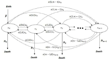
Figure 1: Schematic illustration of tumor cell population model.

$${dx_{0}(t)\over dt}=\underbrace{\beta~{}x_{0}(t)}_{\text{Birth due to mitosis}}+\underbrace{\sum_{j=1}^{m-1}\alpha(j,0)x_{j}(t)}_{\text{transition to $x_{0}$}}-\overbrace{\Big{[}\sum_{k=1}^{m-1}\alpha(0,k)\Big{]}~{}x_{0}(t)}^{\text{transition from $x_{0}$}}-\overbrace{D_{0}~{}x_{0}(t)}^{\text{Death}}$$ (3.1)

and for $i\neq 0$:

$${dx_{i}(t)\over dt}=\underbrace{\displaystyle{\sum_{\underset{j\neq i}{j=0}}^{m-1}\alpha(j,i)~{}x_{j}(t)}}_{\text{transition to $x_{i}$}}-\overbrace{\Big{[}\sum_{\underset{k\neq 1}{k=0}}^{m-1}\alpha(i,k)\Big{]}~{}x_{i}(t)}^{\text{transition from $x_{i}$}}-\overbrace{D_{i}~{}x_{i}(t)}^{\text{Death}}$$ (3.2)

These equations produce the following system:

$${dx_{0}(t)\over dt} = \beta~{}x_{0}(t)+\sum_{j=1}^{m-1}\alpha(j,0)~{}x_{j}(t)-\Big{[}\sum_{k=1}^{m-1}\alpha(0,k)+D_{0}\Big{]}~{}x_{0}(t)$$ (3.3)

$${dx_{1}(t)\over dt} = \displaystyle{\sum_{\underset{j\neq 1}{j=0}}^{m-1}\alpha(j,1)~{}x_{j}(t)}-\displaystyle{\Big{[}\sum_{\underset{k\neq 1}{k=0}}^{m-1}\alpha(1,k)+D_{1}\Big{]}~{}x_{1}(t)}$$

$$\vdots$$

$${dx_{m-1}(t)\over dt} = \sum_{j=0}^{m-2}\alpha(j,m-1)~{}x_{j}(t)-\Big{[}\sum_{k=0}^{m-2}\alpha(m-1,k)+D_{m-1}\Big{]}~{}x_{m-1}(t)$$

4 Model Calibration

The probability that a cell will remain in $x_{0}$ after radiation is $\textbf{P}(0,0)$. Therefore, the average number of births in one day after applying the $k^{th}$ dose fraction and just before the $(k+1)^{th}$ dose fraction is equal to:

$$n(k) = x_{0}(k)\hskip 5.69046pt\mu\hskip 5.69046pt\textbf{P}(0,0)$$ (4.1)

$$= x_{0}(k)\hskip 5.69046pt\mu(1-q)^{m}$$

As seen in Eq. (4.1), the newborn cells’ population size is proportional to $x_{0}$. Therefore, the birth rate can be taken as:

$$\beta=\mu(1-q)^{m}\hskip 5.69046pt$$ (4.2)

Lemma 4.1.

Suppose that a cell has $i$ deactivated target(s) just before the application of a dose fraction and $\Pi=\textbf{PR}$. After treatment and repair,

1. $\Pi(i,j)$ represents the probability that a cell with $i$ deactivated target(s) just before the application of a dose fraction has $j$ deactivated target(s) right before the application of the next dose fraction.

2. An average number of $x_{i}\Pi(i,j)$ cells move from $x_{i}$ into $x_{j}$.

3. For fixed $m$ and $k\geq 1$, the map $i\rightarrow\Pi^{k}(i,m)$ is increasing.

Proof.

1. Suppose that $\Pi=\textbf{PR}$. Therefore:

   $$\Pi(i,j)=\sum_{k=0}^{m}{\textbf{P}(i,k)\textbf{R}(k,j)}$$ (4.3)

   Eq. (2.2) shows that $\textbf{R}(m,j)=0$ for $j<m$. Therefore:

   $$\Pi(i,j)=\sum_{k=0}^{m-1}{\textbf{P}(i,k)\textbf{R}(k,j)}$$ (4.4)

   Now assume that a cell has $i$ deactivated targets just before applying a dose fraction. After radiation and right before the repair mechanism, this cell may remain in subpopulation $x_{i}$ with probability $\textbf{P}(i,i)$, or it may move to subpopulation $x_{k}$, $k=i+1,...,(m-1)$, with probability $\textbf{P}(i,k)$. Following repair, this cell may move from subpopulation $x_{k}$ to subpopulation $x_{j}$ with probability $\textbf{R}(k,j)$. Therefore, the probability of transitioning from subpopulation $x_{i}$ into subpopulation $x_{j}$ after treatment and repair (one day) is $\Pi(i,j)$.
   

2. The effect of treatment and repair on one cell is independent of the rest of the cells. Therefore, the average number of cells moving from subpopulation $x_{i}$ into subpopulation $x_{j}$ is equal to $x_{i}\Pi(i,j)$.

3. See [20].

∎

The following corollary is a direct consequence of lemma (4.1).

Corollary 4.1.

With the same assumptions described in Lemma (4.1):

1. The cells’ transition rate from subpopulation $x_{i}$ into subpopulation $x_{j}$ is equal to $\alpha(i,j)=\Pi(i,j)\hskip 5.69046pt(Day^{-1})$.

2. The death rate of subpopulation $x_{i}$ is $D_{i}=\Pi(i,m)\hskip 5.69046pt(Day^{-1})$.

Remark 4.1.

According to lemma 4.1, we can separate the tumor cells into different sub-populations according to their sensitivity to the radiation. Therefore, the death rate in a subpopulation with more deactivated targets is higher than a subpopulation with fewer deactivated targets, which can be interpreted as the treatment heterogeneity in the model.

Now, starting with subpopulation $x_{0}$, cells give birth at a constant rate of $\mu(1-q)^{m}\hskip 5.69046pt(Day^{-1})$. In addition, cells transit from subpopulation $x_{i}$ into subpopulation $x_{0}$ at a rate of $\Pi(i,0)\hskip 5.69046pt(Day^{-1})$. Conversely, cells move from subpopulation $x_{0}$ into subpopulation $x_{i}$ at a rate of $\Pi(0,i)\hskip 5.69046pt(Day^{-1})$ or may die at a rate of $\Pi(0,m)\hskip 5.69046pt(Day^{-1})$, where $\Pi$ is the transition matrix. Hence, for $i=0,...,(m-1)$ we have:

$${}\sum_{l=0}^{m}\Pi(l,i)=1$$ (4.5)

By substituting Eq. (4.5) in Eq. (3.1) we get:

$${dx_{0}(t)\over dt} = [\Pi(0,0)+\mu(1-q)^{m}-1]~{}x_{0}(t)+\sum_{l=1}^{m-1}{\Pi(l,0)x_{l}(t)}$$ (4.6)

Same analysis shows that for $i=1,\dots,(m-1)$:

$${dx_{i}(t)\over dt} = \displaystyle{\sum_{\underset{l\neq i}{l=0}}^{m-1}\Pi(l,i)~{}x_{l}(t)}-x_{i}(t)~{}\displaystyle{\sum_{\underset{l\neq i}{l=0}}^{m}{\Pi(i,l)}}$$ (4.7)

By substituting Eq. (4.5) in Eq. (3.2) we get:

$${dx_{i}(t)\over dt} = \displaystyle{\sum_{\underset{l\neq i}{l=0}}^{m-1}\Pi(l,i)~{}x_{l}(t)}-x_{i}~{}[1-\Pi(i,i)]$$ (4.8)

Finally, by substituting Eq. (4.6) and Eq. (4.8) in Eq. (3.3), the tumor growth model is described by:

$${dx_{0}(t)\over dt} = [\Pi(0,0)+\mu(1-q)^{m}-1]~{}x_{0}(t)+\sum_{l=1}^{m-1}{\Pi(l,0)x_{l}(t)}$$ (4.9)

$${dx_{1}(t)\over dt} = [\Pi(1,1)-1]~{}x_{1}(t)+\displaystyle{\sum_{\underset{l\neq 1}{l=0}}^{m-1}{\Pi(l,1)x_{l}(t)}}.$$

$$\vdots$$

$${dx_{m-1}(t)\over dt} = [\Pi(m-1,m-1)-1]~{}x_{m-1}(t)+\sum_{l=0}^{m-2}{\Pi(l,m-1)x_{l}(t)}.$$

with initial conditions $\mathrm{x}(0)=(n_{0},0,...,0)^{\top}$.

5 Tumor lifespan

What dose magnitude is required to remove the tumor completely? A small number of cells may still remain after resection, that are not visible and detectable by MRI. Therefore, it is crucial to know how many dose fractions must be applied to eliminate the remaining cancerous cells.
The tumor lifespan is defined as the minimum number of dose fractions required to remove the entire tumor [24]. Therefore, based on tumor population dynamics, the tumor lifespan is defined as:

$$L=\min\{\lfloor t\rfloor:~{}\lfloor N(t)\rfloor=0\}$$ (5.1)

where

$$N(t)=\sum_{l=0}^{m-1}{x_{l}(t)}+n(\lfloor t\rfloor)$$ (5.2)

6 Stability Analysis

Suppose that $m$ is an arbitrary integer. System (4.9) can be written as:

$$\dot{x}(t)=A(q,r)~{}x(t)$$ (6.1)

where matrix $A$ is described as:

$$A_{tk}=\left\{\begin{array}[]{lll}\Pi(0,0)+\mu(1-q)^{m}-1&i,j=0\\ \Pi(i,i)-1&i=j\hskip 14.22636ptand\hskip 14.22636pti\neq 0\\ \Pi(j,i)&i\neq j\end{array}\right.$$ (6.2)

where $t=i+1$ and $k=j+1$. Therefore

$$A_{11}=\Pi(0,0)+\mu(1-q)^{m}-1$$

and for $2\leq t\leq m$

$$A_{tt} = \Pi(t-1,t-1)-1$$

$$= \Pi(i,i)-1$$

Let $A_{m\times m}=(A_{tk})$ be a complex matrix. For $t\in{\{1,...,m\}}$ let $\displaystyle{R_{t}=\sum_{k\neq{t}}\left|A_{tk}\right|}$ denote the sum of the absolute values of the non-diagonal entries in the $t$-th row and $\displaystyle{D(A_{tt},R_{t})}$ be the closed disc centered at $A_{tt}$ with radius $R_{t}$, which is known as Gershgorin disc. Eigenvalue of $A$ lies within at least one of the Gershgorin discs $\displaystyle{D(A_{tt},R_{t})}$ (Gershgorin Theorem [25]).

Lemma 6.1.

Suppose that $B=A^{\top}$. If $R_{t}$ defines as

$$R_{t}=\sum_{k\neq t}{B_{tk}}$$ (6.4)

then

1. $$R_{t}>0$$ (6.5)

2. $$B_{tt}+R_{t}=\left\{\begin{array}[]{ll}\mu(1-q)^{m}-q^{m}&i=0\\ -q^{(m-i)}&1\leq i\leq(m-1)\\ \end{array}\right.$$ (6.8)

Proof.

1. According to (6.2), for $1\leq t\leq m$

   $$R_{t} = \sum_{k\neq t}{B_{tk}}$$ (6.9)

   $$= \sum_{j\neq i}{\Pi(i,j)}$$

   $$> 0$$

2. First consider that $B=A^{\top}$ and $t=1$. Therefore:

   $$\sum_{k=1}^{m}{B_{1k}} = B_{11}+\sum_{k=2}^{m}B_{1k}$$ (6.10)

   $$= \Pi(0,0)+\mu(1-q)^{m}-1+\sum_{j=1}^{m-1}\Pi(0,j)$$

   $$= \Pi(0,0)+\mu(1-q)^{m}-1+(1-\Pi(0,0)-\Pi(0,m))$$

   $$= \mu(1-q)^{m}-q^{m}$$

   Moreover, for $2\leq t\leq m$

   $$\sum_{k=1}^{m}{B_{tk}} = B_{tt}+\sum_{k\neq t}{B_{tk}}$$ (6.11)

   $$= (\Pi(i,i)-1)+\sum_{j\neq i}{\Pi(i,j)}$$

   $$= -\Pi(i,m)$$

   $$= -q^{m-i}$$

∎

The main result of this section is written as follows:

Theorem 6.1.

For any $m\geq 2$, $0<\mu\leq 1$ and $0<r<1$, the system $\mathbf{\dot{x}}=A(q,r)\mathbf{x}$ is stable at equilibrium point $\mathbf{0}$, where $q>0.5$.

Proof.

It is enough to show that all eigenvalues of matrix $A$ have negative real parts . To provide this we will show that for any $q>0.5$, $0<r<1$ and $m\geq 2$ any point of Gershgorin circles $D(A_{tt},R_{t})$ have negative real part, where $1\leq t\leq m$. For this purpose we apply Gershgorin Theorem on matrix $B=A^{\top}$. Based on Lemma (6.1),

$$B_{tt}+R_{t}=\left\{\begin{array}[]{ll}\mu(1-q)^{m}-q^{m}&i=0\\ -q^{(m-i)}&1\leq i\leq(m-1)\\ \end{array}\right.$$ (6.14)

Note that the function $q^{m}$ is an increasing function for $q>0$ and $m$ is an integer. Therefore, for $1-q<0.5<q$ we have:

$$\mu(1-q)^{m}<(1-q)^{m}<q^{m}$$ (6.15)

where $0\leq\mu\leq 1$.
Consequently, $B_{tt}\in\mathbb{R}$ and $B_{tt}+R_{t}<0$ where $q>0.5$ (Figure (2)). This shows that the Gershgorin Circles belong to the left half of real line. In addition, according to Gershgorin Theorem, each eigenvalue of matrix $B$ belongs in one of Gershgorin discs. Therefore, each eigenvalue of matrix $B$ has negative real part. Hence, every eigenvalue of matrix $A$ has negative real part. This completes the proof.

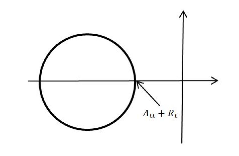
Figure 2: Gershgorin disc $B(A_{tt},R_{t})$.

∎

Theorem 6.2.

Suppose that $m\geq 2$ is an integer, $A\in\mathbb{M}^{m\times m}$ and the set $S$ denotes the value $q$ such that the system (6.1) is stable corresponding to all $0<r<1$ and $0<\mu\leq 1$. Then:

$$\inf_{q}{A}=0.5$$ (6.16)

Proof.

According to Theorem (6.1), the system (4.9) is stable for $q>0.5$. Now for any $\epsilon>0$, corresponding to $q_{0}=0.5-\epsilon$ and for $m=2$ there exists $r_{0}=1-\epsilon$ such that the system (4.9) is unstable. Hence:

$$\inf_{q}{A}=0.5$$ (6.17)

∎

7 Conclusion

In this study, the population dynamics of tumor cells in the process of radiotherapy was examined. A system of differential equations with random variable coefficients was introduced to capture the heterogeneity of cell damage and the repair mechanism between two consecutive dose fractions. Subsequently, a new definition for tumor lifespan was introduced based on tumor population size. Based on the tumor lifespan, the effects of the probability that a target will be inactive after a dose fraction (q) and the probability that a target will reactivate after the repair mechanism (r) were investigated numerically. Our results are in good agreement with previously presented results [20].

References

- [1] Curtis S B. Lethal and potentially lethal lesions induced by radiation–a unified repair model. 1986. Radiat. Res. 106, 252–279.
- [2] Wyman C, Kanaar R. DNA double-strand break repair: all’s well that ends well. Annu. Rev. Genet. 40, 363–383. 2006.
- [3] Hoeijmakers J H. Genome maintenance mechanisms for preventing cancer. Nature 411, 366–374. 2001.
- [4] Zaider M, Minerbo G N. Tumour control probability:a formulation applicable to any temporal protocol of dose delivery. Phys. Med. Biol. 45, 279–293. 2000.
- [5] Dawson A, Hillen T. Derivation of the tumour control probability(TCP) from a cell cycle model. Comput. Math. Methods Med.7, 121–141. 2006.
- [6] Gay H A, Niemierko A. A free program for calculating EUD-based NTCP and TCP in external beam radiotherapy. Phys.Med.23, 115–125. 2007.
- [7] Lyman J T. Complication probability as assessed from dose volume histograms. Radiat. Res. 104, 513–519. 1985.
- [8] Kallman P, Agren A, Brahme A. Tumour and normal tissue responses to fractionated non-uniform dose delivery. Int.J.Radiat.Biol. 62, 249–262. 1992.
- [9] Fowler J, The linear-quadratic formula and progress in fractionated radiotherapy. Br.J.Radiol.62,679–694. 1989.
- [10] Quinn T, Sinkala Z. Dynamics of prostate cancer stem cells with diffusion and organism response. BioSystems, 96(1), 69–79. 2009.
- [11] Sachs R K, Hlatky L R, Hahnfeldt P. Simple ODE models of tumor growth and anti-angiogenic or radiation treatment. Math. Comput. Modell. 33, 1297–1305. 2001.
- [12] Gámez, M., López, I., Garay, J., & Varga, Z. Observation and control in a model of a cell population affected by radiation. Biosystems, 96(2), 172-177. 2009.
- [13] Bastogne T,Samson A,Keinj R,Vallois P,Wantz-Mézières S,Pinel S,Bechet D,Barberi-Heyob M. Phenomenological modeling of tumor diameter growth based on a mixed effects model. J. Theor. Biol. 262, 544–55. 2010.
- [14] Kirkby N F, Burnet N G, Faraday D B F. Mathematical modelling of the response of tumour cells to radiotherapy. Nucl. Instrum. MethodsPhys. Res. Sect. B188, 210–215. 2002.
- [15] Michelson S, Leith J T. Tumor Heterogeneity and Growth Contr. A Survey of Models for Tumor-Immune System Dynamics. Birkuser, pp. 295–333. 1997.
- [16] Rédei G P. Encyclopedia of genetics, genomics, proteomics, and informatics. Springer Science Business Media, Volume 2. 2008.
- [17] Turner M E Some classes of hit-theory models. Mathematical Biosciences, 23(3), 219-235. 1975.
- [18] Nomiya T. Discussions on target theory: past and present. Journal of radiation research, 54(6), 1161-1163. 2013.
- [19] Keinj R, Bastogne T, Vallois P. Multinomial model-based formulations of TCP and NTCP for radiotherapy treatment planning. J.Theor.Biol. 279, 55–62. 2011.
- [20] Keinj R, Bastogne T, Vallois P. Tumor growth modeling based on cell and tumor lifespans. J.Theor.Biol. 312, 76–86. 2012.
- [21] O’Rourke S F C, McAneney H, Hillen T. Linear quadratic and tumour control probability modeling in external beam radiotherapy J. Math. Biol. 58, 799–817. 2009.
- [22] Gupta, P. B., Fillmore, C. M., Jiang, G., Shapira, S. D., Tao, K., Kuperwasser, C., & Lander, E. S. Stochastic state transitions give rise to phenotypic equilibrium in populations of cancer cells. Cell, 146(4), 633–644. 2011.
- [23] Durrett, R., Foo, J., Leder, K., Mayberry, J., & Michor, F. Intratumor heterogeneity in evolutionary models of tumor progression. Genetics, 188(2), 461–477. 2011.
- [24] Oroji, A., Omar, M., & Yarahmadian, S. An Ito stochastic differential equations model for the dynamics of the MCF-7 breast cancer cell line treated by radiotherapy. Journal of theoretical biology, 407, 128–137. 2016.
- [25] Varga, R. S. Geršgorin and his circles (Vol. 36). Springer Science & Business Media. 2010.