Proton fluxes measured by the PAMELA experiment from the minimum to the maximum solar activity for the 24th solar cycle

Abstract

Precise measurements of the time-dependent intensity of the low energy ($<50$ GeV) galactic cosmic rays are fundamental to test and improve the models which describe their propagation inside the heliosphere. Especially, data spanning different solar activity periods, i.e. from minimum to maximum, are needed to achieve comprehensive understanding of such physical phenomenon. The minimum phase between the 23^rd and the 24^th solar cycles was peculiarly long, extending up to the beginning of 2010 and followed by the maximum phase, reached during early 2014. In this paper, we present proton differential spectra measured from January 2010 to February 2014 by the PAMELA experiment. For the first time the galactic cosmic ray proton intensity was studied over a wide energy range (0.08-50 GeV) by a single apparatus from a minimum to a maximum period of solar activity. The large statistics allowed the time variation to be investigated on a nearly monthly basis. Data were compared and interpreted in the context of a state-of-the-art three-dimensional model describing the galactic cosmic rays propagation through the heliosphere.

Matteo Martucci

1 Introduction

The energy spectra of galactic cosmic rays (GCRs), measured at Earth, are significantly influenced by the Sun’s activity. Traversing the heliosphere, GCRs interact with the expanding solar wind and its embedded turbulent magnetic field, undergoing convection, diffusion, adiabatic energy losses and particle drifts because of the global curvature and gradients of the heliospheric magnetic field. As a consequence, the intensity of GCRs at Earth decreases with respect to the GCR energy spectrum outside the heliosphere, Local Interstellar Spectrum (LIS). This solar modulation has large effects on low energy cosmic rays (less than a few GeVs), while the effects gradually subside as the energy increases, becoming negligible above a few tens of GeV (e.g. [Strauss & Potgieter (2014a)]). This modulation mechanism depends on the particle species, their charge and energy per nucleon (or rigidity) and it changes with time, determined by solar activity e.g. following the 11-year cycle and the 22-year magnetic polarity cycle (see also e.g. [Potgieter (2013)]). Precise measurements of GCR spectra, at different phases of the solar cycle, are essential to understand the various processes affecting the propagation of cosmic rays in the heliosphere (e.g. see [Adriani et al. (2017), Bindi et al. (2017)]).

Since the 1950s the variability of the galactic cosmic-ray flux has been constantly monitored by a network of ground-based neutron monitors (e.g. see [Moraal et al. (2000), Shea & Smart (2000), Usoskin et al. (2005)]). However, the intensity of the galactic cosmic rays was indirectly inferred by these detectors measuring the nucleons produced by the nuclear cascade generated by cosmic rays interacting with the atmosphere. The PAMELA (Payload for Antimatter/Matter Exploration and Light-nuclei Astrophysics) space-borne experiment (Picozza, 2007; Boezio, 2009) provided direct measurements of the cosmic ray energy spectra and composition. The apparatus collected data from July 2006 to January 2016, covering the most recent solar activity period, between cycle 23^rd and the current cycle 24^th. Measurements of the proton differential energy spectra provided by the PAMELA instrument during the most recent solar minimum (from mid-2006 to the end of 2009) in the energy range from $80$ MeV to $50$ GeV, have already been published (Adriani et al., 2013). The evolution of the low energy galactic proton spectra on a solar-rotation-time basis (Carrington rotation) was presented, providing the first measurements of the changing solar modulation over a wide energy range and for a very quiet solar minimum. This period showed an extraordinary quiet heliosphere and unusually prolonged minimum. It was expected that the new solar cycle would begin early in 2008, instead minimum modulation conditions continued until the end of 2009. As a consequence, the highest low energy proton intensities since the beginning of the space age was registered during December 2009 (e.g. see Mewaldt et al. (2010)), which was unexpected given the solar magnetic field polarity epoch at that time (e.g. see Potgieter et al. (2013); Strauss & Potgieter (2014b)). Results of a state-of-the-art full three dimensional (3D) model (Potgieter et al., 2014) was used to reproduce the PAMELA observational data. This model was based on the solution of the Parker transport equation, taking into account all the physical processes involved in solar modulation and simulating the solar minimum conditions of the 23/24 cycles (Potgieter et al., 2014; Vos & Potgieter, 2015). Similar studies were conducted on the effects of solar modulation on cosmic ray electrons (Adriani et al., 2015a; Potgieter et al., 2015) from which the dependence of the solar modulation on a particle’s charge sign was observed (Di Felice et al., 2017). Following this extraordinarily deep minimum, the subsequent increase in the solar activity appeared remarkably weak in terms of e.g. sunspot number, solar wind speed and number of solar events (Schroder et al., 2017; Aslam et al., 2015; Jiang et al., 2015). According to various solar activity data, the maximum of cycle 24^th occurred in early 2014, with an estimated changing in the global axial dipole sign taking place in October 2013, while northern and southern polar fields reversing in November 2012 and March 2014, respectively (Sun et al., 2017).

The results presented in this paper refer to the evolution of the proton intensity from the end of the last solar minimum (January 2010) until the maximum of cycle 24^th (February 2014). The evolution of the low energy proton spectrum was studied on a solar rotation period basis, similarly to the previous publication (Adriani et al., 2013).

In the following, a brief description of the mission and details about the data analysis will be presented. Results on the proton flux measurements from 2010 to 2014 in the energy range from 80 MeV - 50 GeV are then presented, compared with the results of the mentioned 3D numerical model simulating the same heliospheric condition of the data-taking period, and discussed in the framework of a solar modulation theory.

2 Instrument and data analysis

After its launch, on June $15$, 2006 the PAMELA experiment had been almost continuously taking data until January 2016. The experiment was located on board the Resurs-DK1 Russian satellite placed by a Soyuz rocket at a highly inclined ($70^{\circ}$) elliptical orbit between $350$ km and $600$ km height, changed into a circular one of $580$ km in September 2010. The satellite quasi-polar orbit allowed the PAMELA instrument to sample low cutoff-rigidity orbital regions for a considerable amount of time, making it suitable for low energy particle studies. The apparatus consisted of a combination of detectors that provided information for particle identification and precise energy measurements. These detectors were (from top to bottom): a Time-of-Flight system; a magnetic spectrometer; an anti-coincidence system; an electromagnetic imaging calorimeter; a shower tail catcher scintillator and a neutron detector. Detailed information about the instrument can be found in (Picozza, 2007; Adriani et al., 2014, 2017).

The proton fluxes were evaluated on a Carrington rotation basis according to the official listing (http://umtof.umd.edu/pm/crn/). No isotopic separation (proton/deuterium) was performed in this analysis. The present analysis spans the period between Carrington rotation 2092 and 2146 (January 2010 - February 2014). Most of these observations took place during a high solar activity period characterized by numerous solar events even if it should be recalled that solar cycle 24 is considerably less active than the three preceding cycles (e.g. see Schroder et al. (2017)). A significant fraction of these events produced high energy particles (mostly protons and Helium nuclei with energies up to a few GeV). This particles reached the Earth orbit and were indistinguishable from the GCR component collected by the PAMELA instrument. For a proper study of the solar modulation of GCRs this solar component had to be excluded. The approach used in this work was to remove the periods in which this contamination was present. Data were excluded for the duration of the solar event using the information recorded by the low energy ($>60$ MeV) proton channel of GOES-15 (ftp://satdat.ngdc.noaa.gov/sem/goes/data/). Solar events have been studied by the PAMELA experiment and have been the topic of other publications (e.g. see Adriani et al. (2015b)). Also the periods of Forbush decreases observed by the PAMELA instrument (e.g. Munini et al. (2017)) were excluded from the analysis.

The analysis procedure used in this work was similar to the one applied to the proton data over the solar minimum period presented and discussed in Adriani et al. (2013). The fluxes were evaluated as follows:

$$\phi(E)=\frac{N(E)}{\epsilon(E)\times G(E)\times T\times\Delta E}$$ (1)

where $N(E)$ is the unfolded count distribution, $\epsilon(E)$ the efficiencies of the particle selections, $G(E)$ the geometrical factor, $T$ the live-time and $\Delta E$ the width of the energy interval.

The large proton statistics permitted the study of the selection efficiencies in-flight for each Carrington rotation. This was particularly relevant for the time dependent track reconstruction efficiency, which varied from $\sim$20$\%$ in December 2009 to $\sim$15$\%$ at the beginning of 2014, because of the sudden failure of some front-end chips of the tracking system (see Adriani et al. (2015a)). This experimental information was combined with Monte Carlo simulation (performed with GEANT4 (Agostinelli et al., 2003)) to properly reproduce the in-flight setup configuration as describe in (Adriani et al., 2011, 2015a).

The geometrical factor, i.e. the requirement of triggering and containment, at least 1.5 mm away from the magnet walls and the TOF-scintillator edges, was estimated with the full simulation of the apparatus and was found to be constant at 19.9 cm² sr. The live time was provided by an on-board clock that timed the periods during which the apparatus was waiting for a trigger.

Both the response of the spectrometer (i.e. the rigidity resolution) and the ionization energy losses suffered by the protons crossing the detector caused a migration of proton events from one energy bin to another. To account for these effects and obtain the unfolded count distribution a Bayesian unfolding procedure, as described in D’Agostini (1995), was applied (see also Adriani et al. (2015a) and Munini (2015)). The detector response matrix was obtained from the simulation and calculated over each Carrington rotation to follow any change in the instrumental setup.

Because of the numerous geomagnetic regions crossed by the satellite over its $\sim$92-minutes orbit, the proton energy spectrum was evaluated for sixteen different vertical geomagnetic cutoff intervals, estimated using the satellite position and the Störmer approximation. The updated (2010) version of the IGRF (https://www.ngdc.noaa.gov/IAGA/vmod/igrf.html) was used. The final fluxes were then evaluated following the approach described in Adriani et al. (2015a).

It was observed that the high energy part of the resulting spectra had a systematic time dependence beyond statistical uncertainties with the fluxes varying of several percent between 2010 and 2014. This was corrected following the procedure adopted in Adriani et al. (2013): the fluxes were normalized at high energy (30-50 GeV) to the proton flux measured over the period July 2006 - March 2008 (i.e. the proton spectrum of Adriani et al. (2011) lowered by $3.2\%$ as explained in Adriani et al. (2013)). The uncertainties on these normalization factors, of the order of one percent, were treated as a systematic uncertainty.

Other systematic uncertainties were due to the efficiencies evaluation and the unfolding procedure as discussed in Adriani et al. (2013); Munini (2015); Adriani et al. (2015a). The total systematic uncertainty shown in Figures 1 and 2 and in Table 1 was obtained quadratically summing the various systematic errors. This systematic uncertainty was about 8$\%$ over the whole energy range and time period.

Figure 1 (top panel a) shows the comparison of the proton fluxes measured during Carrington rotation 2091 (December 7, 2009 - January 3, 2010) obtained in this analysis with the corresponding ones from Adriani et al. (2013). As can be seen from the constant fit performed on the ratio (statistical errors only) between the two results (top panel b), there is an excellent agreement ($\approx 1\%$) over the whole energy range. A similar agreement, Figure 1 bottom panel a, is also found comparing the PAMELA fluxes averaged over the period from May 19, 2011 to November 26, 2013 with the corresponding AMS-02 proton fluxes (Aguilar et al., 2015) taken over the same time period. Bottom panel b shows the ratio between the two measurements along with a constant fit to the data performed above 2 GV. An excellent agreement can be seen at these rigidities. At lower rigidities the PAMELA proton fluxes are systematically higher by about 10$\%$. This discrepancy could be due to differences in data exclusion periods during solar events and Forbush decreases that have major effects below 2 GV.

Figure 1: Top panel: the proton fluxes measured during the Carrington rotation 2091 (December 7, 2009 - January 3, 2010) obtained in this analysis (red circles) and the corresponding one obtained in a previous work (Adriani et al., 2013), (black squares). The error bars are statistical and the shaded area represents the quadratic sum of all systematic uncertainties. The ratio between the two results is shown in panel b as well as the value obtained from a constant fit (dashed black line) performed on this ratio. Errors are statistical only. Bottom panel: the PAMELA fluxes averaged over the period from May 19, 2011 to November 26 2013 compared with concurrent AMS-02 measurement (Aguilar et al., 2015) (panel a). Panel b shows the ratio between the two measurements. P₀ is the result of a linear fit on this flux ratio above 2 GV. Only statistical errors are showed.

3 Results

A total of 36 proton energy spectra were obtained from the minimum to the maximum activity of solar cycle 24. Data from the Carrington rotations number 2095 to the 2102 are missing because of a system shut-down for satellite maintenance operations. Moreover, the Carrington rotations number 2113, 2115, 2121, 2123, 2125, 2126, 2135, 2136, 2137, 2143, 2145 are also missing because of the presence of solar energetic particles as previous explained.

Figure 2 (panels a,b,c) shows the time profiles of the proton fluxes for three illustrative energy intervals along with the HCS tilt angle data obtained with radial boundary conditions taken from Wilcox Solar Observatory at http://wso.stanford.edu/. (panel d). The red shaded areas represent the systematic uncertainties while the error bars represent the statistical errors. Starting from late 2009, the tilt angle rapidly increased from low values typical for a period of solar minimum activity reaching its maximum value in mid 2012. During this time period the proton fluxes between 0.08-0.095 GeV and between 0.67-0.72 GeV showed a sharp decrease of about a factor 4 and about 2.5 respectively, Figure 2 panels a and b. These large values of the tilt angle had basically been maintained, except for a few relatively short periods of decreased values, until the end of 2013. After this period, the tilt angle has decreased systematically, indicating that solar modulation has turned around to enter a new solar minimum epoch. The proton flux after mid 2012 continued to decrease until February 2014 when it reached its minimum intensity. In this time window the fluxes between 0.08-0.095 GeV and between 0.67-0.72 GeV decreased by about a factor 2.2 and by about a factor 1.4 respectively, Figure 2 panels a and b. As expected between 36.7-40 GeV, Figure 2 panel c, the proton flux is constant with time.

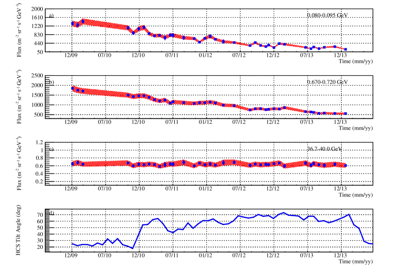
Figure 2: The time profile of the proton flux for three energy intervals: 0.08-0.095 GeV (panel a), 0.67-0.72 GeV (panel b) and 36.7-40 GeV (panel c) along with the time profile of the tilt angle obtained with radial boundary conditions taken from Wilcox Solar Observatory at http://wso.stanford.edu/ (panel d). The error bars indicate the statistical errors while the shaded area the systematic uncertainties.

Figure 3 (left panel) shows the totality of the proton fluxes evaluated from January 3, 2010 (blue data points) until February 11, 2014 (red data points) on a Carringoton rotation basis. The right panel of Figure 3 shows the variation of the proton intensities with respect to the first Carrington rotation of 2010. The energy dependence of the solar modulation is particularly evident from this figure: the low energy protons are the most affected with a decrease of nearly a factor 10 from the minimum to the maximum solar activity while above $\sim$ 30 GV the proton fluxes do not show any temporal variation within the measurement uncertainties. Table 1 presents the galactic proton spectra measured by the PAMELA experiment over four time periods. These data illustrate how the proton spectra evolved from early 2010 to early 2014. The complete data set can be found at the ASI Space Science Data Center, where all the proton energy spectra are retrievable from the Cosmic Ray Data Base (http://tools.asdc.asi.it/CosmicRays/chargedCosmicRays.jsp).

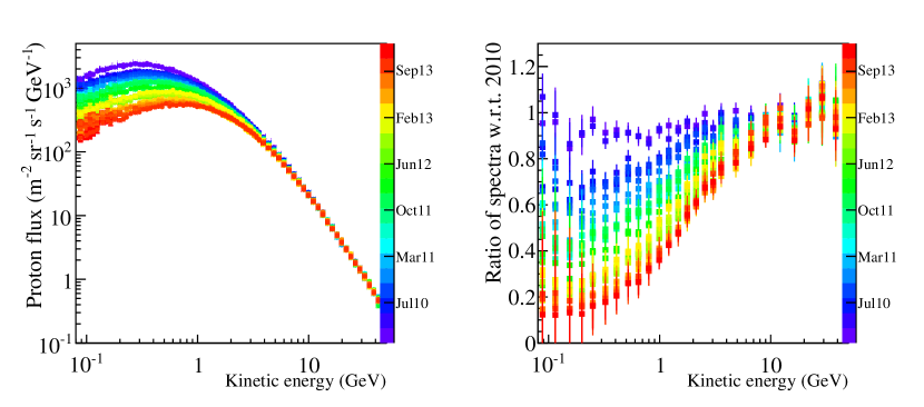
Figure 3: Left panel: the evolution of the proton spectra from the minimum to the maximum activity of solar cycle 24, from January 2010 (blue), to February 2014 (red). Right panel: the variation of the proton differential intensity with respect to the first proton spectrum of 2010.

4 Data interpretation and discussion

As shown in Figure 3 left panel the observed spectra became progressively harder with increasing solar activity as fewer low energy protons were able to reach the Earth. The spectral peaks (turning point in the value of the maximum flux of each spectrum) consequently shifted systematically to higher energy values. From 2010 to 2014 the kinetic energy value of the peak shifted from about 350 MeV to 700 MeV. The adiabatic energy loss signature (spectral shape below the turn-energy proportional to E) became therefore more evident with solar maximum spectra. This confirms that adiabatic energy losses for protons (and GCR nuclei) are a significantly important part of the solar modulation process in the heliosphere (see also Potgieter & Vos (2017)).

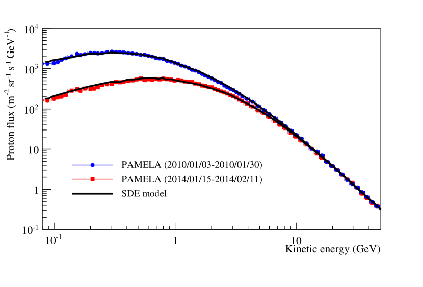
Figure 4: PAMELA proton spectra registered in two Carrington rotations during 2010 (blue circles) and 2014 (red squares). Stochastic differential equations (SDE) model (black dashed curve) is superimposed to the observational data.

In Figure 4 the PAMELA proton spectra measured in January 2010 and in early 2014 are overlaid with the corresponding computed spectra. A full 3D numerical model based on solving Parker’s transport equation (Parker, 1965) with the so-called stochastic differential equation approach was used to compute the proton differential intensity at Earth. This modeling approach and its validation against proton observations from PAMELA for the period 2006 to 2009 was published in detail by Raath et al. (2016). For a description of a global approach to the modeling of GCR’s in the heliosphere, see also Potgieter (2017).

The assumed LIS for protons is chosen according to Vos & Potgieter (2015). The modulation volume is assumed to be spherical with the heliopause (HP) position at 122 AU. The HP is considered to be the outer modulation boundary. For the period 2010 to 2014, changes in the heliospheric current sheet’s tilt angle, as shown in Figure 2 panel d, are incorporated into the model together with corresponding changes in the magnitude of the solar magnetic field B as observed at the Earth. These values were averaged for at least the previous 12 months as representation of estimated modulation conditions in the heliosphere for the prior year. This is based on the average time it takes for the frozen-in magnetic field and tilt angles to propagate from the Sun to the HP, being carried outward at the average speed of the solar wind. These averaged values therefore represent a proxy for the global modulation conditions that prevailed throughout the heliosphere for the time periods considered here. The three diffusion coefficients in this 3D approach are parallel and perpendicular, in the radial and polar directions, to the global magnetic field, and are assumed to scale as 1/B, which is the most straight forward approach from a diffusion theory point of view. This follows the basic modelling approach described also by Potgieter et al. (2015). The drift coefficient scales also as 1/B, assuming weak scattering as explained by Ngoben & Potgieter (2015).

These computed spectra for 2010 and 2014 are shown in Figure 4 together with the corresponding observations. Evidently, the model reproduces the features of the two spectra well over this wide energy range, in particular the intensity values where the spectra peak and how this peak shifts to higher energies while the spectrum decreases with increased modulation. Reproducing the 2010 spectrum (during an A$<$0 magnetic polarity cycle) required relatively minor changes to the modulation parameters used by Raath et al. (2016). However, in order to reproduce the 2014 spectrum (during an A$>$0 magnetic polarity cycle), with the amount of modulation additionally occurring as shown in Figure 3, the diffusion coefficients had to be decreased by a factor of 2 with respect to the 2010 values. Simultaneously, the drift coefficient had to be reduced to only 10% of the solar minimum value. This illustrates that reproducing the total amount of modulation occurring from maximum GCR intensity in early 2010 to minimum intensity in 2014 requires about a factor of 2 increase in the effectiveness of diffusion while drifts had to be significantly reduced, otherwise the intensity levels would have remained far too high with increasing solar modulation for this A$>$0 magnetic cycle.

5 Conclusion

The observations presented here illustrate the total modulation that had occurred from minimum modulation (highest intensity) of GCRs to maximum modulation (lowest intensity) under a relatively quiet Sun and subsequently also the heliosphere. This provides a unique opportunity to study the modulation of GCRs under such extraordinary conditions. In particular, combined with the observed electron to positron ratios reported by PAMELA in Adriani et al. (2016), it provides information useful to understand how diffusion and drifts effects vary with time and energy.

Table 1: Proton flux measured by PAMELA over four time periods. The first and second errors represent the statistical and systematic uncertainties, respectively.

Kinetic Energy (GeV)		Flux(m2 s sr GeV)-1
	2010/01/03-2010/01/30	2011/04/12-2011/05/09	2012/08/15-2012/09/11	2014/01/15-2014/02/15
0.082-0.095	1334.967 $\pm$ 82.677 $\pm$ 127.149	795.308 $\pm$ 47.742 $\pm$ 76.072	333.947 $\pm$ 40.400 $\pm$ 36.724	164.583 $\pm$ 25.663 $\pm$ 18.902
0.095-0.105	1382.404 $\pm$ 96.083 $\pm$ 133.199	836.770 $\pm$ 55.939 $\pm$ 81.172	415.946 $\pm$ 51.653 $\pm$ 45.755	181.962 $\pm$ 30.565 $\pm$ 21.320
0.105-0.110	1462.203 $\pm$ 138.301 $\pm$ 148.366	939.265 $\pm$ 83.015 $\pm$ 95.267	345.066 $\pm$ 65.980 $\pm$ 43.123	199.548 $\pm$ 44.385 $\pm$ 25.410
0.110-0.120	1682.318 $\pm$ 103.829 $\pm$ 157.830	979.690 $\pm$ 59.402 $\pm$ 92.551	438.529 $\pm$ 51.925 $\pm$ 46.809	205.254 $\pm$ 31.346 $\pm$ 22.790
0.120-0.130	1816.430 $\pm$ 106.984 $\pm$ 149.757	963.679 $\pm$ 58.432 $\pm$ 81.848	494.574 $\pm$ 54.318 $\pm$ 47.484	223.106 $\pm$ 32.338 $\pm$ 23.175
0.130-0.150	2040.187 $\pm$ 79.696 $\pm$ 180.845	1075.864 $\pm$ 43.351 $\pm$ 96.031	552.629 $\pm$ 40.069 $\pm$ 52.988	286.300 $\pm$ 25.680 $\pm$ 28.578
0.150-0.160	2343.113 $\pm$ 119.948 $\pm$ 214.642	1046.064 $\pm$ 59.954 $\pm$ 96.757	542.123 $\pm$ 55.489 $\pm$ 55.293	309.547 $\pm$ 37.346 $\pm$ 32.766
0.160-0.170	2185.130 $\pm$ 114.921 $\pm$ 199.299	1151.039 $\pm$ 62.378 $\pm$ 105.827	602.654 $\pm$ 58.035 $\pm$ 60.533	287.579 $\pm$ 35.579 $\pm$ 30.646
0.170-0.190	2302.665 $\pm$ 82.801 $\pm$ 201.218	1179.811 $\pm$ 44.381 $\pm$ 103.910	625.510 $\pm$ 41.630 $\pm$ 58.856	322.769 $\pm$ 26.411 $\pm$ 31.053
0.190-0.210	2484.283 $\pm$ 85.461 $\pm$ 215.673	1304.952 $\pm$ 46.483 $\pm$ 114.144	668.770 $\pm$ 42.942 $\pm$ 62.440	314.053 $\pm$ 25.881 $\pm$ 30.283
0.210-0.220	2469.407 $\pm$ 82.545 $\pm$ 220.425	1282.348 $\pm$ 44.210 $\pm$ 115.907	635.254 $\pm$ 39.659 $\pm$ 61.927	322.497 $\pm$ 24.950 $\pm$ 32.828
0.220-0.240	2404.784 $\pm$ 57.377 $\pm$ 207.994	1323.680 $\pm$ 31.696 $\pm$ 115.256	643.178 $\pm$ 28.150 $\pm$ 59.086	347.635 $\pm$ 18.215 $\pm$ 32.578
0.240-0.260	2452.868 $\pm$ 57.790 $\pm$ 211.535	1381.816 $\pm$ 32.343 $\pm$ 119.807	703.898 $\pm$ 29.401 $\pm$ 64.278	395.317 $\pm$ 19.325 $\pm$ 36.942
0.260-0.290	2587.382 $\pm$ 48.354 $\pm$ 219.281	1382.849 $\pm$ 26.389 $\pm$ 118.183	744.302 $\pm$ 24.665 $\pm$ 66.175	411.836 $\pm$ 16.033 $\pm$ 37.071
0.290-0.310	2660.621 $\pm$ 59.944 $\pm$ 228.362	1411.766 $\pm$ 32.628 $\pm$ 122.150	742.029 $\pm$ 30.165 $\pm$ 67.279	420.169 $\pm$ 19.762 $\pm$ 38.487
0.310-0.340	2614.418 $\pm$ 48.414 $\pm$ 221.109	1405.834 $\pm$ 26.549 $\pm$ 119.878	734.236 $\pm$ 24.507 $\pm$ 65.126	465.419 $\pm$ 16.922 $\pm$ 41.386
0.340-0.360	2600.506 $\pm$ 59.064 $\pm$ 222.681	1427.089 $\pm$ 32.739 $\pm$ 123.237	740.257 $\pm$ 30.166 $\pm$ 66.846	460.405 $\pm$ 20.562 $\pm$ 41.725
0.360-0.390	2549.032 $\pm$ 47.743 $\pm$ 215.811	1412.139 $\pm$ 26.604 $\pm$ 120.255	774.639 $\pm$ 25.225 $\pm$ 68.524	476.739 $\pm$ 17.072 $\pm$ 41.993
0.390-0.430	2443.305 $\pm$ 40.470 $\pm$ 205.093	1414.240 $\pm$ 23.069 $\pm$ 119.391	751.346 $\pm$ 21.516 $\pm$ 65.442	500.676 $\pm$ 15.152 $\pm$ 43.648
0.430-0.460	2393.106 $\pm$ 46.216 $\pm$ 202.300	1386.433 $\pm$ 26.386 $\pm$ 118.106	779.713 $\pm$ 25.300 $\pm$ 68.331	512.399 $\pm$ 17.702 $\pm$ 45.058
0.460-0.500	2328.825 $\pm$ 39.511 $\pm$ 195.569	1426.760 $\pm$ 23.225 $\pm$ 120.411	770.670 $\pm$ 21.819 $\pm$ 66.803	540.540 $\pm$ 15.766 $\pm$ 46.855
0.500-0.540	2201.917 $\pm$ 38.488 $\pm$ 185.090	1358.087 $\pm$ 22.725 $\pm$ 114.736	773.471 $\pm$ 21.932 $\pm$ 67.123	571.107 $\pm$ 16.240 $\pm$ 49.419
0.540-0.580	2232.442 $\pm$ 38.796 $\pm$ 187.522	1312.368 $\pm$ 22.390 $\pm$ 110.961	774.749 $\pm$ 22.017 $\pm$ 67.089	518.287 $\pm$ 15.498 $\pm$ 44.889
0.580-0.620	2110.885 $\pm$ 37.741 $\pm$ 177.592	1308.983 $\pm$ 22.407 $\pm$ 110.699	759.016 $\pm$ 21.854 $\pm$ 65.851	546.131 $\pm$ 15.941 $\pm$ 47.238
0.620-0.670	2013.549 $\pm$ 32.989 $\pm$ 168.502	1272.052 $\pm$ 19.810 $\pm$ 107.028	776.185 $\pm$ 19.833 $\pm$ 66.748	532.933 $\pm$ 14.124 $\pm$ 45.789
0.670-0.720	1843.377 $\pm$ 31.596 $\pm$ 154.484	1198.768 $\pm$ 19.288 $\pm$ 101.059	739.141 $\pm$ 19.425 $\pm$ 63.661	556.023 $\pm$ 14.472 $\pm$ 47.701
0.720-0.770	1802.870 $\pm$ 31.308 $\pm$ 151.032	1124.218 $\pm$ 18.736 $\pm$ 94.805	718.388 $\pm$ 19.226 $\pm$ 61.941	542.074 $\pm$ 14.337 $\pm$ 46.560
0.770-0.830	1749.204 $\pm$ 28.240 $\pm$ 146.298	1121.779 $\pm$ 17.137 $\pm$ 94.240	719.320 $\pm$ 17.639 $\pm$ 61.656	567.905 $\pm$ 13.440 $\pm$ 48.460
0.830-0.890	1570.682 $\pm$ 26.852 $\pm$ 131.498	1087.582 $\pm$ 16.923 $\pm$ 91.463	711.780 $\pm$ 17.622 $\pm$ 61.110	548.560 $\pm$ 13.250 $\pm$ 46.785
0.890-0.960	1500.112 $\pm$ 24.349 $\pm$ 125.310	1038.532 $\pm$ 15.345 $\pm$ 87.093	663.605 $\pm$ 15.808 $\pm$ 56.763	537.129 $\pm$ 12.168 $\pm$ 45.622
0.960-1.020	1409.334 $\pm$ 19.521 $\pm$ 118.330	936.771 $\pm$ 12.030 $\pm$ 79.009	646.067 $\pm$ 12.807 $\pm$ 55.601	507.792 $\pm$ 9.730 $\pm$ 43.461
1.020-1.090	1335.055 $\pm$ 17.609 $\pm$ 111.752	897.745 $\pm$ 10.933 $\pm$ 75.526	622.088 $\pm$ 11.675 $\pm$ 53.337	525.043 $\pm$ 9.184 $\pm$ 44.684
1.090-1.170	1194.435 $\pm$ 15.600 $\pm$ 99.908	860.732 $\pm$ 10.040 $\pm$ 72.209	600.630 $\pm$ 10.772 $\pm$ 51.347	511.695 $\pm$ 8.505 $\pm$ 43.441
1.170-1.250	1130.494 $\pm$ 15.201 $\pm$ 94.684	789.504 $\pm$ 9.640 $\pm$ 66.367	561.511 $\pm$ 10.457 $\pm$ 48.076	480.355 $\pm$ 8.265 $\pm$ 40.828
1.250-1.340	1043.878 $\pm$ 13.799 $\pm$ 87.331	726.467 $\pm$ 8.740 $\pm$ 61.020	548.761 $\pm$ 9.786 $\pm$ 46.897	469.432 $\pm$ 7.728 $\pm$ 39.799
1.340-1.420	938.592 $\pm$ 13.907 $\pm$ 78.904	721.208 $\pm$ 9.258 $\pm$ 60.809	496.622 $\pm$ 9.909 $\pm$ 42.723	465.878 $\pm$ 8.191 $\pm$ 39.672
1.420-1.520	895.874 $\pm$ 12.176 $\pm$ 75.005	662.716 $\pm$ 7.953 $\pm$ 55.659	488.957 $\pm$ 8.819 $\pm$ 41.800	428.841 $\pm$ 7.047 $\pm$ 36.392
1.520-1.620	818.801 $\pm$ 11.657 $\pm$ 68.713	606.027 $\pm$ 7.616 $\pm$ 51.005	445.967 $\pm$ 8.440 $\pm$ 38.274	411.672 $\pm$ 6.917 $\pm$ 34.947
1.620-1.720	741.816 $\pm$ 11.099 $\pm$ 62.396	562.603 $\pm$ 7.341 $\pm$ 47.396	435.086 $\pm$ 8.343 $\pm$ 37.298	382.659 $\pm$ 6.672 $\pm$ 32.581
1.720-1.830	673.281 $\pm$ 10.082 $\pm$ 56.557	525.954 $\pm$ 6.769 $\pm$ 44.300	391.637 $\pm$ 7.549 $\pm$ 33.642	375.139 $\pm$ 6.299 $\pm$ 31.831
1.830-1.950	631.863 $\pm$ 9.364 $\pm$ 53.079	490.276 $\pm$ 6.265 $\pm$ 41.286	370.506 $\pm$ 7.034 $\pm$ 31.736	348.823 $\pm$ 5.823 $\pm$ 29.618
1.950-2.070	575.142 $\pm$ 8.955 $\pm$ 48.483	431.415 $\pm$ 5.888 $\pm$ 36.422	340.164 $\pm$ 6.748 $\pm$ 29.239	346.174 $\pm$ 5.814 $\pm$ 29.424
2.070-2.200	519.375 $\pm$ 7.169 $\pm$ 43.745	415.325 $\pm$ 4.927 $\pm$ 35.038	332.828 $\pm$ 5.681 $\pm$ 28.518	316.716 $\pm$ 4.726 $\pm$ 26.912
2.200-2.330	468.252 $\pm$ 6.822 $\pm$ 39.547	381.339 $\pm$ 4.730 $\pm$ 32.242	314.474 $\pm$ 5.533 $\pm$ 27.009	293.339 $\pm$ 4.559 $\pm$ 24.986
2.330-2.480	442.058 $\pm$ 6.183 $\pm$ 37.266	338.366 $\pm$ 4.155 $\pm$ 28.567	290.548 $\pm$ 4.963 $\pm$ 24.913	272.463 $\pm$ 4.097 $\pm$ 23.155
2.480-2.620	382.832 $\pm$ 5.963 $\pm$ 32.457	314.857 $\pm$ 4.152 $\pm$ 26.688	271.590 $\pm$ 4.974 $\pm$ 23.412	258.542 $\pm$ 4.132 $\pm$ 22.078
2.620-2.780	346.394 $\pm$ 5.307 $\pm$ 29.322	294.360 $\pm$ 3.757 $\pm$ 24.897	250.850 $\pm$ 4.477 $\pm$ 21.578	241.663 $\pm$ 3.736 $\pm$ 20.586
2.780-2.940	317.209 $\pm$ 5.076 $\pm$ 26.883	264.513 $\pm$ 3.561 $\pm$ 22.461	223.179 $\pm$ 4.225 $\pm$ 19.268	218.276 $\pm$ 3.549 $\pm$ 18.634
2.940-3.120	295.253 $\pm$ 4.613 $\pm$ 25.014	241.820 $\pm$ 3.209 $\pm$ 20.506	206.612 $\pm$ 3.834 $\pm$ 17.809	206.426 $\pm$ 3.255 $\pm$ 17.594
3.120-3.300	262.302 $\pm$ 4.347 $\pm$ 22.278	216.080 $\pm$ 3.034 $\pm$ 18.367	188.554 $\pm$ 3.667 $\pm$ 16.281	191.244 $\pm$ 3.136 $\pm$ 16.322
3.300-3.490	238.599 $\pm$ 4.036 $\pm$ 20.280	201.418 $\pm$ 2.851 $\pm$ 17.135	179.749 $\pm$ 3.487 $\pm$ 15.538	170.347 $\pm$ 2.884 $\pm$ 14.573
3.490-3.690	204.508 $\pm$ 3.642 $\pm$ 17.442	185.956 $\pm$ 2.670 $\pm$ 15.843	162.815 $\pm$ 3.235 $\pm$ 14.113	155.731 $\pm$ 2.689 $\pm$ 13.353
3.690-4.120	178.114 $\pm$ 2.322 $\pm$ 14.930	153.363 $\pm$ 1.656 $\pm$ 12.850	139.847 $\pm$ 2.047 $\pm$ 11.850	136.054 $\pm$ 1.717 $\pm$ 11.440
4.120-4.590	150.564 $\pm$ 2.046 $\pm$ 12.646	128.540 $\pm$ 1.453 $\pm$ 10.794	114.930 $\pm$ 1.778 $\pm$ 9.773	115.714 $\pm$ 1.517 $\pm$ 9.753
4.590-5.110	117.786 $\pm$ 1.723 $\pm$ 9.924	103.522 $\pm$ 1.241 $\pm$ 8.711	95.778 $\pm$ 1.544 $\pm$ 8.163	92.180 $\pm$ 1.288 $\pm$ 7.787
5.110-5.680	94.763 $\pm$ 1.475 $\pm$ 8.008	85.760 $\pm$ 1.079 $\pm$ 7.239	80.949 $\pm$ 1.355 $\pm$ 6.919	79.408 $\pm$ 1.141 $\pm$ 6.725
5.680-6.300	74.839 $\pm$ 1.255 $\pm$ 6.340	66.203 $\pm$ 0.909 $\pm$ 5.605	64.084 $\pm$ 1.155 $\pm$ 5.497	62.411 $\pm$ 0.968 $\pm$ 5.300
6.300-6.990	59.473 $\pm$ 1.059 $\pm$ 5.048	53.257 $\pm$ 0.773 $\pm$ 4.516	50.253 $\pm$ 0.970 $\pm$ 4.319	50.251 $\pm$ 0.824 $\pm$ 4.273
6.990-7.740	45.962 $\pm$ 0.893 $\pm$ 3.925	43.370 $\pm$ 0.670 $\pm$ 3.693	42.767 $\pm$ 0.859 $\pm$ 3.688	40.426 $\pm$ 0.710 $\pm$ 3.455
7.740-8.570	37.064 $\pm$ 0.763 $\pm$ 3.170	35.503 $\pm$ 0.577 $\pm$ 3.030	32.609 $\pm$ 0.713 $\pm$ 2.826	33.508 $\pm$ 0.616 $\pm$ 2.868
8.570-9.480	28.753 $\pm$ 0.512 $\pm$ 2.471	25.887 $\pm$ 0.379 $\pm$ 2.222	26.297 $\pm$ 0.492 $\pm$ 2.286	25.380 $\pm$ 0.408 $\pm$ 2.184
9.480-10.480	22.697 $\pm$ 0.435 $\pm$ 1.956	21.708 $\pm$ 0.331 $\pm$ 1.867	21.052 $\pm$ 0.420 $\pm$ 1.840	20.517 $\pm$ 0.350 $\pm$ 1.773
10.480-11.570	18.376 $\pm$ 0.375 $\pm$ 1.594	17.469 $\pm$ 0.284 $\pm$ 1.512	17.000 $\pm$ 0.361 $\pm$ 1.493	16.431 $\pm$ 0.300 $\pm$ 1.426
11.570-12.770	13.985 $\pm$ 0.312 $\pm$ 1.218	13.673 $\pm$ 0.239 $\pm$ 1.187	13.349 $\pm$ 0.304 $\pm$ 1.177	13.135 $\pm$ 0.256 $\pm$ 1.145
12.770-14.090	10.229 $\pm$ 0.255 $\pm$ 0.899	10.112 $\pm$ 0.196 $\pm$ 0.884	10.645 $\pm$ 0.259 $\pm$ 0.944	10.221 $\pm$ 0.216 $\pm$ 0.896
14.090-15.540	8.623 $\pm$ 0.223 $\pm$ 0.761	8.455 $\pm$ 0.171 $\pm$ 0.741	8.362 $\pm$ 0.219 $\pm$ 0.747	7.718 $\pm$ 0.179 $\pm$ 0.680
15.540-17.120	6.927 $\pm$ 0.192 $\pm$ 0.613	6.545 $\pm$ 0.144 $\pm$ 0.577	6.278 $\pm$ 0.182 $\pm$ 0.564	6.095 $\pm$ 0.152 $\pm$ 0.540
17.120-18.860	4.854 $\pm$ 0.153 $\pm$ 0.432	5.109 $\pm$ 0.121 $\pm$ 0.453	5.067 $\pm$ 0.156 $\pm$ 0.458	4.840 $\pm$ 0.129 $\pm$ 0.432
18.860-20.760	3.811 $\pm$ 0.129 $\pm$ 0.343	3.756 $\pm$ 0.099 $\pm$ 0.337	3.958 $\pm$ 0.132 $\pm$ 0.361	3.805 $\pm$ 0.110 $\pm$ 0.342
20.760-22.850	2.998 $\pm$ 0.091 $\pm$ 0.272	2.950 $\pm$ 0.072 $\pm$ 0.266	2.933 $\pm$ 0.093 $\pm$ 0.271	3.044 $\pm$ 0.080 $\pm$ 0.276
22.850-25.150	2.332 $\pm$ 0.076 $\pm$ 0.214	2.318 $\pm$ 0.061 $\pm$ 0.211	2.209 $\pm$ 0.077 $\pm$ 0.208	2.307 $\pm$ 0.066 $\pm$ 0.212
25.150-27.660	1.712 $\pm$ 0.063 $\pm$ 0.159	1.770 $\pm$ 0.051 $\pm$ 0.163	1.741 $\pm$ 0.065 $\pm$ 0.165	1.753 $\pm$ 0.055 $\pm$ 0.162
27.660-30.420	1.358 $\pm$ 0.053 $\pm$ 0.128	1.497 $\pm$ 0.045 $\pm$ 0.139	1.448 $\pm$ 0.057 $\pm$ 0.138	1.445 $\pm$ 0.048 $\pm$ 0.135
30.420-33.440	1.111 $\pm$ 0.046 $\pm$ 0.105	1.149 $\pm$ 0.038 $\pm$ 0.108	1.141 $\pm$ 0.048 $\pm$ 0.111	1.116 $\pm$ 0.040 $\pm$ 0.105
33.440-36.750	0.850 $\pm$ 0.038 $\pm$ 0.082	0.840 $\pm$ 0.031 $\pm$ 0.080	0.799 $\pm$ 0.039 $\pm$ 0.080	0.787 $\pm$ 0.032 $\pm$ 0.075
36.750-40.390	0.653 $\pm$ 0.032 $\pm$ 0.064	0.585 $\pm$ 0.024 $\pm$ 0.057	0.613 $\pm$ 0.032 $\pm$ 0.062	0.607 $\pm$ 0.027 $\pm$ 0.060
40.390-44.370	0.485 $\pm$ 0.026 $\pm$ 0.048	0.465 $\pm$ 0.021 $\pm$ 0.046	0.442 $\pm$ 0.026 $\pm$ 0.046	0.460 $\pm$ 0.022 $\pm$ 0.046
44.370-48.740	0.376 $\pm$ 0.022 $\pm$ 0.038	0.389 $\pm$ 0.018 $\pm$ 0.039	0.368 $\pm$ 0.023 $\pm$ 0.038	0.386 $\pm$ 0.019 $\pm$ 0.039

References

- Adriani et al. (2011) Adriani, O., et al. 2011, Science, 332, 69
- Adriani et al. (2013) Adriani, O., et al. 2013, ApJ, 765, 91
- Adriani et al. (2014) Adriani, O., et al. 2014, Phys. Rep., 544, 4
- Adriani et al. (2015a) Adriani, O., et al. 2015a, ApJ, 810, 142
- Adriani et al. (2015b) Adriani, O., et al. 2015b, ApJ, 801, L3
- Adriani et al. (2016) Adriani, O., et al. 2016, Phys. Rev. Lett., 116, 241105
- Adriani et al. (2017) Adriani, O. et al. 2017, RIVISTA DEL NUOVO CIMENTO, 40, 473
- Aguilar et al. (2015) Aguilar, M., et al. 2015, PRL, 114, 171103
- Agostinelli et al. (2003) Agostinelli, S., et al. 2003, Nuclear Instruments and Methods in Physics Research A, 506, 250
- Aslam et al. (2015) O. P. M. Aslam et al. Sol. Phys., 290:2333–2353, August 2015.
- Bindi et al. (2017) Bindi, V., Corti, C., Consolandi, C., Hoffman, J., Whitman, K. 2017, Adv Space Res., 60, 865
- Boezio (2009) Boezio, M., et al. 2009, New J. Phys., 11, 105023
- Bruno et al. (2017) Bruno, A., et al. 2017, ApJl.
- Carrington (1863) Carrington, R, C, Monthly Notices of the Royal Astronomical Society, 23, 203, April 1863.
- D’Agostini (1995) D’Agostini, G 1995, Nuclear Instruments and Methods in Physics Research A, 362, 487
- Hathaway (2015) Hathaway, D. H. 2015, Living Rev. Solar Phys., 12, 4
- Hoeksema (1992) Hoeksema, J. T. 1992, Solar Wind Seven Colloquium, edited by E. Marsch and R. Schwenn, 1992.
- Jiang et al. (2015) J. Aslam et al. ApJ Lett., 808:L28, July 2015.
- Mewaldt et al. (2010) Mewaldt, R. A. et al., Ap. J. Lett., 723, L1, 2010.
- Moraal et al. (2000) Moraal, H., A. et al., Space Sci. Rev., 93, 285, 2000.
- Munini (2015) Munini, R. 2015, PhD thesis, Universitá degli Studi di Trieste, Italy, http://pamela.roma2.infn.it
- Munini et al. (2017) Munini, R., et al. 2017, submitted to ApJ,
- Ngoben & Potgieter (2015) Ngobeni, M. D. and Potgieter, M. S., 2015, Adv. Sp. Res., 56, 1525
- Parker (1965) Parker, E. N., 1965, ApJ, 142, 1086
- Picozza (2007) Picozza, P., et al. 2007, ApJ, 27, 296
- Potgieter (2013) Potgieter, M. S. 2013, Living Rev. Solar Phys., 10, 3
- Potgieter et al. (2013) Potgieter, M. S., et al. 2013, Proc. of the 33rd Int. Cosmic Ray Conf. (Rio de Janeiro. Brazil)
- Potgieter et al. (2014) Potgieter, M. S., et al. 2014, Sol. Phys., 289, 1
- Potgieter et al. (2015) Potgieter, M. S., et al. 2015, ApJ, 810, 141
- Potgieter (2017) Potgieter, M. S. 2017, ASR, 60, 4
- Potgieter & Vos (2017) Potgieter, M. S. and Vos, E. E : 2017, A&A, 601, A23
- Raath et al. (2016) Raath, J. L., et al. 2016, Adv. Sp. Res., 57, 9
- Di Felice et al. (2017) Di Felice, V et al. 2017, ApJ, 834, 89
- Schroder et al. (2017) Schroder, K. P., et al. 2017, Monthly Notices of the Royal Astr. Soc., 470, 1.
- Shea & Smart (2000) Shea, M. A., and D. F. Smart, Space Sci. Rev., 93, 229, 2000
- Strauss & Potgieter (2014a) Strauss, R. D. and Potgieter M. S. 2014a, Adv. Sp. Res. 53, 1015
- Strauss & Potgieter (2014b) Strauss, R. D. and Potgieter M. S. 2014b, Sol. Phys., 289, 3197
- Sun et al. (2017) Sun, X., et al. 2015, ApJ, 798, 114
- Usoskin et al. (2005) Usoskin I. G., Alanko-Huotari K., Kovaltsov G. A., Mursula K., Jour. of Geophys. Res. Space Phys., 110, A12108, 2005
- Vos & Potgieter (2015) Vos, E.E., and Potgieter, M. S. 2015, ApJ, 815, 119