Selective cooling by impulse perturbations in a simple toy model

Abstract

We show in a simple exactly-solvable toy model that a properly designed impulse perturbation can transiently cool down low-energy degrees of freedom at the expenses of high-energy ones that heat up. The model consists of two infinite-range quantum Ising models, one, the high-energy sector, with a transverse field much bigger than the other, the low-energy sector. The finite-duration perturbation is a spin-exchange that couples the two Ising models with an oscillating coupling strength. We find a cooling of the low-energy sector that is optimised by the oscillation frequency in resonance with the spin-exchange excitation. After the perturbation is turned off, the Ising model with low transverse field can even develop spontaneous symmetry-breaking despite being initially above the critical temperature.

Crystalline solids, either metallic or insulating, are characterised by electronic and lattice degrees of freedom whose dynamics is controlled by a hierarchy of energy scales and relaxation times that are directly accessible by pump-probe spectroscopyGiannetti et al. (2016); Nicoletti and Cavalleri (2016). In such experiments, a sample is driven away from equilibrium by an intense laser pulse, the pump, and the subsequent relaxation dynamics is probed by a variety of spectroscopic tools as function of the time delay from the pump pulse, with a resolution that today can well achieve the attosecondCorkum and Krausz (2007). Selected degrees of freedom can be excited by properly tuning the laser frequency, thus offering an unprecedented wide choice of non-equilibrium pathways unaccessible by conventional experiments where thermodynamic state variables, like temperature, pressure or chemical composition, are varied. Moreover, the early-time relaxation dynamics is essentially unaffected by the environment, which starts playing a role only nanoseconds after the pulse. In other words, the environment just determines the initial equilibrium conditions of the sample, which then evolves for a relatively long time as it were effectively isolated. This is just what happens in cold atoms systemsLangen et al. (2015), with the major difference that real materials are more complex, and thus potentially much richer though harder to model.
As an example, we here mention a recent pump-probe experiment on K₃C₆₀ alkali fullerides Mitrano et al. (2016). When shot by a laser pulse in the mid-infrared, $80-200$ meV, frequency range, this molecular conductor, which at equilibrium becomes a superconductor below $T_{c}\sim 20~{}\text{K}$, shows a transient, few picoseconds long, superconducting-like optical response that is observed up to temperatures $T\sim 200~{}\text{K}$, ten times higher than $T_{c}$. Bearing in mind that in K₃C₆₀, as in many other correlated superconductorsBasov et al. (2011), the transition to a normal metal occurs by gap filling rather than closing, the transient superconducting signal looks as if the laser pulse had swept away the thermal excitations that at equilibrium fill the gapNava et al. (2017). In other words, it appears that the light promotes the excitations responsible of the mid-infrared absorption, but, at the same time, it cools down the low frequency, $\lesssim 20~{}\text{meV}$, electronic degrees of freedom. An explanation of this selective cooling was proposed in Ref. Nava et al. (2017) based on the prediction that the mid-infrared absorption is due to a localised spin-triplet exciton that can be populated by light through the concurrent absorption/emission of spin-triplet particle-hole excitations of the Fermi liquid. Since at equilibrium the thermal population of spin-triplet particle-hole pairs is more abundant than that of the excitons, the net effect is an entropy flow from the former to the latter within the pulse duration. After the pulse ends, that entropy slowly flows back by the non-radiative exciton recombination, which entails the existence of a whole time interval in which the Fermi liquid is effectively cooler than at equilibrium, in agreement with the experimental evidence.

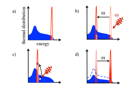
Figure 1: Pictorial explanation of the cooling mechanism within the rotating-wave approximation (RWA). a) The initial thermal distribution of low-energy (blue) and high-energy (red) excitations; b) a laser pulse with frequency $\omega$ shoots the system. In the RWA the high-energy peak is effectively shifted downward by $\omega$ for the whole pulse duration; c) the amplitude of the laser induces a transfer of thermal excitations to the formerly poorly-populated peak; d) when the laser is turned off, the peak returns back to its initial position, but it is now overpopulated at the expenses of the low-energy excitations.

Such cooling mechanism is in fact quite genericBernier et al. (2009), as it requires, in essence, the existence of an entropy sink that opens when the laser is on, while, when the laser is turned off, it gradually gives back the stolen entropy. A simple-minded pictorial explanation within the rotating-wave approximation is drawn in Fig. 1. Here we shall show how to practically achieve such cooling in a simple exactly-solvable toy model.
Specifically, we consider the following unperturbed Hamiltonian

$$H=\sum_{n=1}^{2}\,H_{n}\,,$$ (1)

where, for each $n=1,2$,

$$H_{n} =-\frac{\displaystyle J_{n}}{\displaystyle 2V}\,\sum_{\mathbf{R}\mathbf{R^{\prime}}}\,\sigma^{x}_{n\mathbf{R}}\,\sigma^{x}_{n\mathbf{R^{\prime}}}-h_{n}\,\sum_{\mathbf{R}}\,\sigma^{z}_{n\mathbf{R}}\,,$$ (2)

describes an infinite-range quantum Ising model, a special case of the so-called Lipkin-Meshkov-Glick modelLipkin et al. (1965), $V\!=\!2M$ is the number of sites, while $\sigma^{a}_{n\mathbf{R}}$ is the $a=x,y,z$ component of the $n=1,2$ Ising spin at site $\mathbf{R}$. For simplicity we shall take $J_{1}=J_{2}=1$ as energy unit.
The model (2) for each $n=1,2$ admits as conserved quantity the total spin with eigenvalue $\text{S}_{n}(\text{S}_{n}+1)$, where $\text{S}_{n}=0,1,\dots,M$. Each energy eigenstate is thus labelled also by a value of $\text{S}_{n}$ and its degeneracy $g(\text{S}_{n})=C^{2M}_{S_{n}}-C^{2M}_{S_{n}+1}$, where $C^{n}_{m}$ are binomial coefficients, corresponds to the number of ways $2M$ spin-1/2’s can give a total spin $\text{S}_{n}$. If we set $\text{S}_{n}=MN_{n}$, then, in the thermodynamic limit $M\to\infty$, $N_{n}$ effectively becomes a continuous variable $\in[0,1]$ and the partition function can be evaluated semiclassicallyLieb (1973); Das et al. (2006); Bapst and Semerjian (2012)

$$\!\!\!Z_{n}=\text{e}^{-\beta F_{n}}\!=\!\sum_{\text{S}_{n}}\,g(\text{S}_{n})\!\!\!\sum_{\text{S}_{n}^{z}=-\text{S}_{n}}^{\text{S}_{n}}\!\!\langle\text{S}_{n},\text{S}_{n}^{z}\!\mid\!\text{e}^{-\beta\,H_{n}}\!\mid\!\text{S}_{n},\text{S}_{n}^{z}\rangle$$

$$\;\;\simeq M\!\int_{0}^{1}\!\!\!dN_{n}\big{(}2\text{S}_{n}+1\big{)}\!\int\frac{\displaystyle d\cos\theta_{n}\,d\phi_{n}}{\displaystyle 4\pi}\,\text{e}^{-2M\beta f_{n}},$$ (3)

where the semiclassical free-energy density reads

$$f_{n}\!=\!-\frac{\displaystyle N_{n}^{2}}{\displaystyle 2}\sin^{2}\theta_{n}\cos^{2}\phi_{n}-h_{n}N_{n}\cos\theta_{n}-T\mathcal{S}\big{(}N_{n}\big{)}\,,$$ (4)

with the entropy density

$$\mathcal{S}\big{(}N_{n}\big{)} =\frac{\displaystyle\ln g(\text{S}_{n})}{\displaystyle 2M}\simeq\ln 2-\big{(}1+N_{n}\big{)}\ln\sqrt{1+N_{n}}$$ (5)

$$\qquad-\big{(}1-N_{n}\big{)}\ln\sqrt{1-N_{n}}\,,$$

which vanishes at $N_{n}=1$, and increases with decreasing $N_{n}$ up to $\ln 2$ at $N_{n}=0$. In the thermodynamic limit the partition function is dominated by the saddle point of (4), which also implies that at any temperature $T$ the Boltzmann density matrix becomes a projector onto the ground state $\mid\!\text{GS}_{n};N_{n}\rangle$ within the subspace with $N_{n}=N_{n}(T)$Bapst and Semerjian (2012). One readily findsBapst and Semerjian (2012) that, if $h_{n}\leq J_{n}=1$ and $T\leq T_{nc}$, where

$$T_{nc}=2h_{n}\Big{/}\ln\frac{\displaystyle 1+h_{n}}{\displaystyle 1-h_{n}}\;,$$ (6)

then $N_{n}(T)$ is the solution of the equation

$$N_{n}(T)=\tanh\beta\,N_{n}(T)\geq h_{n}\,,$$ (7)

and in the ground state $\mid\!\text{GS}_{n};N_{n}(T)\rangle$ the $Z_{2}$ symmetry, $\sigma^{x}_{n\mathbf{R}}\to-\sigma^{x}_{n\mathbf{R}}$, $\forall\,\mathbf{R}$, of the model (2) is spontaneously broken with order parameter $\langle\,\sigma^{x}_{n\mathbf{R}}\,\rangle^{2}=N_{n}(T)^{2}-h_{n}^{2}$, which corresponds to the Euler angles $\theta_{n}=\cos^{-1}h_{n}/N_{n}(T)$ and $\phi_{n}=0$ in Eq. (4). Above $T_{nc}$, or if $h_{n}>1$, the symmetry is restored, i.e. $\langle\,\sigma^{x}_{n\mathbf{R}}\,\rangle^{2}=0$, $\theta_{n}=0$, and

$$N_{n}(T)=\tanh\beta\,h_{n}\,.$$ (8)

The above semiclassical results, which are exact in the thermodynamic limit, can be rederived by a mean-field density matrix $\rho_{n}=\prod_{\mathbf{R}}\,\rho_{n\mathbf{R}}$, such that $\text{Tr}\big{(}\rho_{n\mathbf{R}}\big{)}=1$, through the variational principle

$$F_{n}\leq\min_{\{\rho_{n\mathbf{R}}\}}\!\!\bigg{(}\text{Tr}\Big{(}\rho_{n}\,H_{n}\Big{)}+T\sum_{\mathbf{R}}\text{Tr}\Big{(}\rho_{n\mathbf{R}}\,\ln\rho_{n\mathbf{R}}\Big{)}\bigg{)}\,.$$ (9)

The above inequality becomes a true equality in the thermodynamic limit because of the infinite connectivity, which implies that, for $\mathbf{R}\not=\mathbf{R^{\prime}}$, $\langle\sigma^{a}_{n\mathbf{R}}\,\sigma^{b}_{n\mathbf{R^{\prime}}}\rangle-\langle\sigma^{a}_{n\mathbf{R}}\rangle\langle\sigma^{b}_{n\mathbf{R^{\prime}}}\rangle\sim 1/M$ and thus vanishes for $M\to\infty$. Minimising the right hand side of Eq. (9), one readily findsSup that

$$\rho_{n\mathbf{R}}(T) =Z_{n\mathbf{R}}^{-1}\;U_{n\mathbf{R}}\,\text{e}^{-\beta\,H_{n\mathbf{R}}(T)}\;U_{n\mathbf{R}}^{\dagger}\,,$$ (10)

where $U_{n\mathbf{R}}=\exp\Big{(}\!-i\phi_{n}\,\sigma^{z}_{n\mathbf{R}}/2\Big{)}\exp\Big{(}\!-i\theta_{n}\,\sigma^{y}_{n\mathbf{R}}/2\Big{)}$, with the same Euler angles as before, and

$$H_{n\mathbf{R}}(T)=-\mu_{n}(T)\,\sigma^{z}_{n\mathbf{R}}\,,$$ (11)

so that $Z_{n\mathbf{R}}=2\cosh\beta\mu_{n}(T)$. The effective field $\mu_{n}(T)=N_{n}(T)$ if $h_{n}\leq 1$ and $T\leq T_{nc}$, otherwise $\mu_{n}(T)=h_{n}$. This variational scheme leads to the same free energy as in the semiclassical approach, but provides additional useful information, for instance that the energy of an excitation that changes $\text{S}_{n}$ by $\pm 1$ is simply $\mp 2\mu_{n}(T)$. We end mentioning that, even though the variational density matrix does not commute, as expected, with the total spin operator, nonetheless its relative fluctuation vanish in the thermodynamic limit.

Coming back to the full unperturbed Hamiltonian (1), we can for a start conclude that the Boltzmann density matrix can be well approximated by

$$\rho=\prod_{\mathbf{R}}\,\rho_{1\mathbf{R}}(T)\,\rho_{2\mathbf{R}}(T)\,,$$ (12)

with $\rho_{n\mathbf{R}}(T)$ of Eq. (10). Since our aim is to describe two coupled systems with degrees of freedom well separated in energy, we choose as Hamiltonian parameters $h_{1}<1$ and $h_{2}\gg 1$, so that $\mu_{2}(T)\gg\mu_{1}(T)$, see Eq. (11), and the subsystem 2 is disordered at any temperature. The phase diagram is shown in Fig. 2.

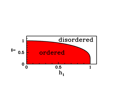
Figure 2: Phase diagram of the Hamiltonian (1) with $h_{2}=10$ as a function of $h_{1}$. In the red coloured region below the critical temperature $T_{c}$ the $Z_{2}$ symmetry of subsystem 1 is spontaneously broken.

In Fig. 3 we plot the temperature dependence of $N_{1}$ and $N_{2}$, see equations (7) and (8), and of the corresponding entropies $\mathcal{S}(N_{n})$, Eq. (5), for $h_{1}=0.5$ and $h_{2}=10$. We note the existence of a wide temperature range, which extends from well below $T_{c}$ to well above it, where subsystem 2 is poor in entropy, $\mathcal{S}(N_{2})\ll 1$, unlike subsystem 1, $\mathcal{S}(N_{1})\lesssim\ln 2$. For our purposes this is a favourable circumstance, as we can exploit subsystem 2 as entropy sink of subsystem 1. We therefore assume that initially, $t=0$, the system is prepared into the thermal state at temperature $T$ and then, from $t=0$ until $t=\tau$ the Hamiltonian changes into $H+\delta H(t)$, where the perturbation

$$\delta H(t)=-E_{0}\,\cos\omega t\,\sum_{\mathbf{R}}\,\sigma^{x}_{1\mathbf{R}}\,\sigma^{x}_{2\mathbf{R}}\,,$$ (13)

mimics a laser pulse of duration $\tau$, frequency $\omega$ and peak amplitude $E_{0}$. Above $t=\tau$ the perturbation is turned off and the system evolves unitarily, again with Hamiltonian $H$ in (1).

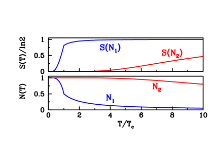
Figure 3: $N_{1}$ and $N_{2}$ (bottom panel) and the corresponding entropies, $\mathcal{S}(N_{n})$ (top panel), as function of temperature for $h_{1}=0.5$ and $h_{2}=10$.

In presence of the perturbation, $\text{S}_{1}=MN_{1}$ and $\text{S}_{2}=MN_{2}$ are not anymore conserved quantities, since $\delta H(t)$ changes both $\text{S}_{1}$ and $\text{S}_{2}$ by $\pm 1$. If $T$ is such that $N_{2}\simeq 1\gg N_{1}$, see Fig. 3, we expect that in the early stage $\delta H(t)$ lowers $\text{S}_{2}$ while raises $\text{S}_{1}$ through a sequence of elementary excitations $\text{S}_{2}\to\text{S}_{2}-1$ and $\text{S}_{1}\to\text{S}_{1}+1$, each with energy cost $\Delta=2\mu_{2}(T)-2\mu_{1}(T)$, see Eq. (11). Therefore, after the pulse stops and if $\tau$ is not too large, a net flow of entropy has occurred from subsystem 1 to 2, which thus corresponds to an effective cooling of the former and corresponding heating of the latter.
To confirm this expectation, we study the time evolution $\rho(t)$ of the density matrix (12), which, because of the infinite connectivity, can be still written as $\rho(t)=\prod_{\mathbf{R}}\,\rho_{\mathbf{R}}(t)$, where $\rho_{\mathbf{R}}(t)$ satisfies the equation of motion ($\hbar=1$) $i\,\dot{\rho}_{\mathbf{R}}(t)=\Big{[}H_{\mathbf{R}}(t)\,,\,\rho_{\mathbf{R}}(t)\Big{]}$, with boundary condition $\rho_{\mathbf{R}}(t=0)=\rho_{1\mathbf{R}}(T)\,\rho_{2\mathbf{R}}(T)$, and where

$$H_{\mathbf{R}}(t)\!=\!-\sum_{n=1}^{2}\Big{(}h_{n}\,\sigma^{z}_{n\mathbf{R}}+m_{n}(t)\,\sigma^{x}_{n\mathbf{R}}\Big{)}\!-\!E(t)\,\sigma^{x}_{1\mathbf{R}}\,\sigma^{x}_{2\mathbf{R}}\,,$$

being $E(t)=E_{0}\cos\omega t$ if $0<t\leq\tau$, and $E(t)=0$ otherwise. The time-dependent fields $m_{n}(t)$, $n=1,2$, are determined by the self-consistency condition $m_{n}(t)=\text{Tr}\Big{(}\rho_{\mathbf{R}}(t)\,\sigma^{x}_{n\mathbf{R}}\Big{)}$, $\forall\,\mathbf{R}$. The equations of motion can be numerically integrated with no particular difficultySup , and therefore we here quote just the outcomes.
In the top panel of Fig. 4 we show $N_{1}(t)$ and $N_{2}(t)$ for $h_{1}=0.5$, $h_{2}=10$, $T=1.1\,T_{c}$, $\tau=3$, $E_{0}=0.4$, and three different frequencies $\omega=18,19,20$. We observe that the maximum increase of $N_{1}(\tau)$ occurs when $\omega=19$, while for $\omega=18$ the increase is lower and for $\omega=20$ we even find a decrease. This is not surprising since $\omega=19$ is exactly in resonance with the excitation that lowers $\text{S}_{2}$ by one and concurrently increases $\text{S}_{1}$ by the same amount, and which indeed costs energy $\Delta=2\mu_{2}(T)-2\mu_{1}(T)=2h_{2}-2h_{1}=19$.

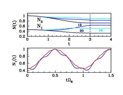
Figure 4: Top panel: time evolution of $N_{1}(t)$, the three lower curves, and $N_{2}(t)$, the three upper ones, for $h_{1}=0.5$, $h_{2}=10$, $T=1.1\,T_{c}$, $\tau=3$, $E_{0}=0.4$ and $\omega=18$, cyan lines, $\omega=19$, blue, and finally $\omega=20$, dark blue. We emphasise that beyond $\tau$, the vertical dashed line, $N_{n}(t)$ remain constant. Bottom panel: time evolution of $N_{1}(t)$ with the same $h_{1}$, $h_{2}$ and $T$ as before, $\omega=\Delta$, but now with a large $\tau$ and two different values of $E_{0}$: $E_{0}=0.5$, blue, and $E_{0}=0.2$, red. We note clear Rabi oscillations, with $\Omega_{\text{R}}=E_{0}/2\pi$ the Rabi frequency.

Hereafter we shall thus stick to resonance, $\omega=\Delta$. In the bottom panel of Fig. 4 we instead plot $N_{1}(t)$ for a large value of $\tau$, the same $h_{1}$ and $h_{2}$ as before, and two different values of $E_{0}=0.5,0.2$. The time is shown in units of the inverse Rabi frequency $\Omega_{\text{R}}=E_{0}/2\pi$. We clearly observe Rabi oscillations, so that, if our aim is to fix the pulse duration so as to get the maximum increase of $N_{1}(t)$ in the minimum $\tau$, then the best choice is $\tau$ around half of the Rabi period, which we shall adopt in what follows.
In Fig. 5, top panel, we show the energy density $E_{1}(t)=\text{Tr}\big{(}\rho(t)\,H_{1}\big{)}/V$ for different initial temperatures, from above to below $T_{c}$. Recalling that $E_{1}(t)$ remains constant for $t\geq\tau$, the results shown imply a significant cooling down of subsystem 1 after the pulse ends. This is evidently counterbalanced by a concurrent heating of subsystem 2, as shown in the bottom panel of Fig. 5.

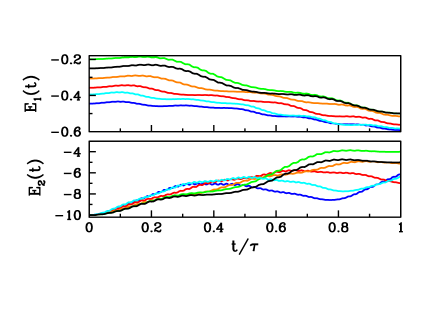
Figure 5: Time evolution of the internal energy $E_{1}(t)$ of subsystem 1, top panel, and $E_{2}(t)$ of subsystem 2, bottom panel, at $h_{1}=0.5$, $h_{2}=10$, $E_{0}=0.5$, the frequency $\omega=\Delta$ at resonance, and different temperatures, $T/T_{c}=1.2,1.0,0.94,0.90,0.86,0.80$, from the upper to the lower curve in the top panel. In the bottom panel the colours correspond to the same $T$ as in the top one.

In view of the above results, we can conceive the possibility to start with subsystem 1 in the disordered phase above $T_{c}$ and end up, after the pulse, in its symmetry broken phase. When the perturbation is turned off, the subsystem 1 evolves unitarily with the Hamiltonian $H_{1}$ in (2), which is equivalent to the classical motion in a potentialDas et al. (2006); Bapst and Semerjian (2012); Mazza and Fabrizio (2012); Sciolla and Biroli (2013)

$$V(m)=-\frac{\displaystyle N_{1}(\tau)^{2}}{\displaystyle 2}\,m^{2}-h_{1}\,N_{1}(\tau)\,\sqrt{1-m^{2}\;}\;,$$ (14)

where $m=\langle\sigma^{x}_{1\mathbf{R}}\rangle\in[-1,1]$ is the order parameter. The necessary condition for symmetry breaking to occur is that the potential (14) has a double well, which requires $N_{1}(\tau)>h_{1}$. This is indeed well possible, see Fig. 4. However, this is not sufficient; one also needs the conserved energy $E_{1}(\tau)$ to be lower than the top of the barrier separating the two minima $E_{*}(\tau)=V(0)=-N_{1}(\tau)\,h_{1}$, the broken-symmetry edge of Ref. Mazza and Fabrizio (2012). If this indeed happens, then the system will end up after the pulse into one of the two equivalent wells and keep oscillating around the minimum, which would imply a finite time-average value of the order parameter. In Fig. 6 we show an explicit case where that occurs, despite the initial temperature being greater than $T_{c}$, $T=1.1\,T_{c}$.

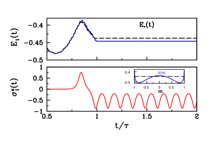
Figure 6: Top panel: time evolution of $E_{1}(t)$, blue solid curve, and $E_{*}(t)=-N_{1}(t)\,h_{1}$, black dashed one, for $h_{1}=0.5$, $h_{2}=2$, $\omega=\Delta$, $E_{0}=0.1$ and the initial $T=1.1\,T_{c}$. Bottom panel: corresponding evolution of the order parameter $\sigma^{x}_{1}(t)$. In the inset we show the classical potential after $t=\tau$ as well as the energy $E_{1}(\tau)$, dashed horizontal line.

In the top panel we plot $E_{1}(t)$, blue solid curve, and $E_{*}(t)$, dashed black one. Indeed, at the end of the pulse the system has $E_{1}(\tau)<E_{*}(\tau)$. In the bottom panel we show the time evolution of the order parameter $\sigma^{x}_{1}(t)$, which, after the pulse, is found to oscillate in the left well with negative average value.
In real materials low- and high-energy degrees of freedom, here represented by subsystems 1 and 2, respectively, are never decoupled from each other before and after the pulse, as we assume with model (1). Therefore, some time after the pulse, the longer the weaker the coupling is, the excess energy acquired by subsystem 2 must flow back to 1 till the two equilibrate to a thermal stationary state. Such thermalisation never occurs with mean-field Hamiltonians like (1). Nonetheless, we may wonder how the previous results change if already in the unperturbed Hamiltonian the two subsystems are coupled to each other. To that end, we changedSup $H$ of (1) into $H-\lambda\sum_{\mathbf{R}}\,\sigma^{x}_{1\mathbf{R}}\,\sigma^{x}_{2\mathbf{R}}$, with a very small time-independent $\lambda=0.01$. The equilibrium phase diagram is practically unchanged by such a tiny $\lambda$ with respect to Fig. 2, with the only difference that now the finite $\langle\sigma^{x}_{1\mathbf{R}}\rangle$ induces also a finite $\langle\sigma^{x}_{2\mathbf{R}}\rangle\sim\lambda\,\langle\sigma^{x}_{1\mathbf{R}}\rangle/h_{2}\ll 1$. In Fig. 7 we show the time evolution of the order parameter $\sigma^{x}_{1}(t)$ with the same Hamiltonian parameters of Fig. 6 but now with $\lambda\not=0$. We note that shortly after the pulse end, top panel, the behaviour is the same as for $\lambda=0$, bottom panel in Fig. 6. However, for longer times, the small but finite $\lambda$ starts playing a role, energy flows back to subsystem 1 and eventually the order parameter vanishes on average, bottom panel in Fig. 7. In spite of that, there does exist a sizeable time interval after the pulse where the system looks as it were ordered, albeit $T>T_{c}$.
We finally remark that the circumstance that the system gets trapped after the pulse into one of the symmetry variant subspaces depends critically on $\tau$. This is evident from Fig. 6, showing that a smaller $\tau$, below the peak in $E_{1}(t)$ at $t\sim 0.8\,\tau$, would not lead to the same result. We find that the trapping occurs most likely when the pulse stops just after the system, in its semiclassical motion, has jumped from one well into the other, which requires a sudden increase in energy to surpass the barrier and seems to be followed by $E_{1}(t)$ overshooting $E_{*}(t)$. We believe that in more realistic models endowed with dissipative channels that provide frictional forces to the semiclassical motion, such transient trapping into an ordered phase would still occur and not require too much fine-tuning of the pulse parameters.

In conclusion, we have shown in an exactly solvable toy model that a properly designed impulse perturbation can produce an effective cooling of low-energy degrees of freedom at the expenses of high-energy ones that heat up. The model is extremely simple, but the mechanism is so generic that it may work even in more realistic situations, like in the case of photo-excited alkali-doped K₃C₆₀ fullerides as suggested in Ref. Nava et al. (2017).

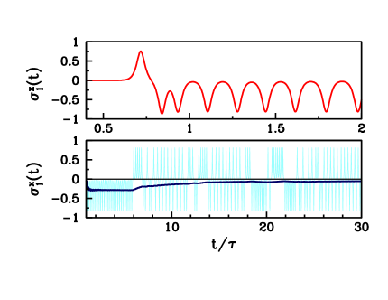
Figure 7: Top panel: same as in Fig. 6 but in presence of a very small coupling $\lambda=10^{-2}$ between the two subsystems. Bottom panel: evolution of the order parameter for longer times. The solid dark blue line is the time-average value of $\sigma^{x}_{1}(t)$.

We are grateful to Erio Tosatti and Alessandro Silva for useful comments and discussions. This work has been supported by the European Union under H2020 Framework Programs, ERC Advanced Grant No. 692670 “FIRSTORM”.

References

- Giannetti et al. (2016) C. Giannetti, M. Capone, D. Fausti, M. Fabrizio, F. Parmigiani, and D. Mihailovic, Advances in Physics 65, 58 (2016), eprint https://doi.org/10.1080/00018732.2016.1194044, URL https://doi.org/10.1080/00018732.2016.1194044.
- Nicoletti and Cavalleri (2016) D. Nicoletti and A. Cavalleri, Adv. Opt. Photon. 8, 401 (2016), URL http://aop.osa.org/abstract.cfm?URI=aop-8-3-401.
- Corkum and Krausz (2007) P. B. Corkum and F. Krausz, Nature Physics 3, 381 EP (2007), URL http://dx.doi.org/10.1038/nphys620.
- Langen et al. (2015) T. Langen, R. Geiger, and J. Schmiedmayer, Annual Review of Condensed Matter Physics 6, 201 (2015), eprint https://doi.org/10.1146/annurev-conmatphys-031214-014548, URL https://doi.org/10.1146/annurev-conmatphys-031214-014548.
- Mitrano et al. (2016) M. Mitrano, A. Cantaluppi, D. Nicoletti, S. Kaiser, A. Perucchi, S. Lupi, P. Di Pietro, D. Pontiroli, M. Riccò, S. R. Clark, et al., Nature 530, 461 (2016), URL http://dx.doi.org/10.1038/nature16522.
- Basov et al. (2011) D. N. Basov, R. D. Averitt, D. van der Marel, M. Dressel, and K. Haule, Rev. Mod. Phys. 83, 471 (2011), URL https://link.aps.org/doi/10.1103/RevModPhys.83.471.
- Nava et al. (2017) A. Nava, C. Giannetti, A. Georges, E. Tosatti, and M. Fabrizio, Nature Physics pp. EP – (2017), URL http://dx.doi.org/10.1038/nphys4288.
- Bernier et al. (2009) J.-S. Bernier, C. Kollath, A. Georges, L. De Leo, F. Gerbier, C. Salomon, and M. Köhl, Phys. Rev. A 79, 061601 (2009), propose a cooling mechanism whose physical principle is close to that of Ref. Nava et al. (2017), though in the different context of cold atom systems, URL https://link.aps.org/doi/10.1103/PhysRevA.79.061601.
- Lipkin et al. (1965) H. Lipkin, N. Meshkov, and A. Glick, Nuclear Physics 62, 188 (1965), ISSN 0029-5582, URL http://www.sciencedirect.com/science/article/pii/002955826590862X.
- Lieb (1973) E. Lieb, Communications in Mathematical Physics 31, 327 (1973), ISSN 0010-3616, URL http://dx.doi.org/10.1007/BF01646493.
- Das et al. (2006) A. Das, K. Sengupta, D. Sen, and B. K. Chakrabarti, Phys. Rev. B 74, 144423 (2006), URL https://link.aps.org/doi/10.1103/PhysRevB.74.144423.
- Bapst and Semerjian (2012) V. Bapst and G. Semerjian, Journal of Statistical Mechanics: Theory and Experiment 2012, P06007 (2012), URL http://stacks.iop.org/1742-5468/2012/i=06/a=P06007.
- (13) See Supplemental Material at … for the derivation of the variational results and of the equations of motion, whose numerical integration lead to the results shown in figures 4–7, which also includes Ref. Brankin and Gladwell (1997).
- Mazza and Fabrizio (2012) G. Mazza and M. Fabrizio, Phys. Rev. B 86, 184303 (2012), URL https://link.aps.org/doi/10.1103/PhysRevB.86.184303.
- Sciolla and Biroli (2013) B. Sciolla and G. Biroli, Phys. Rev. B 88, 201110 (2013), URL https://link.aps.org/doi/10.1103/PhysRevB.88.201110.
- Brankin and Gladwell (1997) R. W. Brankin and I. Gladwell, ACM Trans. Math. Softw. 23, 402 (1997), ISSN 0098-3500, URL http://doi.acm.org/10.1145/275323.275328.