A high-performance analog Max-SAT solver and its application to Ramsey numbers

Abstract

We introduce a continuous-time analog solver for MaxSAT, a quintessential class of NP-hard discrete optimization problems, where the task is to find a truth assignment for a set of Boolean variables satisfying the maximum number of given logical constraints. We show that the scaling of an invariant of the solver’s dynamics, the escape rate, as function of the number of unsatisfied clauses can predict the global optimum value, often well before reaching the corresponding state. We demonstrate the performance of the solver on hard MaxSAT competition problems. We then consider the two-color Ramsey number $R(m,m)$ problem, translate it to SAT, and apply our algorithm to the still unknown $R(5,5)$. We find edge colorings without monochromatic 5-cliques for complete graphs up to 42 vertices, while on 43 vertices we find colorings with only two monochromatic 5-cliques, the best coloring found so far, supporting the conjecture that $R(5,5)=43$.

Digital computing, or Turing’s model of universal computing is currently the reigning computational paradigm. However, there are large classes of problems that are intractable on digital computers, requiring resources (time, memory and/or hardware) for their solution that scale exponentially in the input size of the problem (NP-hard) MertensMoore . Such problems, unfortunately, are abundant in sciences and engineering, for example, the ground-state problem of spin-glasses in statistical physics JPhysA_B82 ; STOC_I00 , the traveling salesman problem TSP , protein folding prot , bioinformatics bioinf , medical imaging biomed1 ; biomed2 , scheduling GJ90 , design debugging, FPGA routing FPGA , probabilistic reasoning ProbReas1 ; ProbReas2 , etc. As CMOS-based digital computing is reaching its limits Moore , alternative approaches are being explored, such as analog computing and quantum computing. While the latter seems promising, there are fundamental physics challenges that still need to be solved before it realizes its potential, leaving analog computing as a currently exploitable option. Although it was explored in the ’50s, it has been abandoned in the favor of the digital approach, due to the technical challenges it posed; for a historical survey on analog machines see Ulmann . By now, however, technology matured enough to control well the physics at the small-scale and thus it makes worthwhile revisiting the analog branch of computing, at least at an application-specific level. For this reason, there has been an increasing effort dedicated recently to analog computing methods and devices specialized to address certain classes of problems Inagaki ; Takata ; McMahon ; Marandi ; Gert ; Indiveri ; Suman ; Parihar ; Emre ; Zohar1 ; Zohar2 ; Ventra ; Traversa ; Adel ; Gauthier ; Stanley ; Compiler . However, there have been recent advances also in general purpose analog computing, see the reviews Pekka ; MacLennan ; Olivier0 ; Olivier1 , and in analog computability theory Olivier1 ; Olivier2 ; Kia .

Here we focus on fully analog (continuous-time) systems, in which both the state variables $\bm{s}=(s_{1},\ldots,s_{N})$ and the time variable $t$ are real numbers, $s_{i}\in\mathbb{R}$, $t\in\mathbb{R}$, updated continuously by the algorithm (software), in form of a set of ordinary differential equations (ODEs) $d\bm{s}/dt=\bm{F}(\bm{s}(t),t)$, $t\in\mathbb{R}$, Olivier1 . The process of computation is interpreted as the evolution of the trajectory (the solution to the ODEs) $\bm{s}(t)=\bm{\Psi}_{t}(\bm{s}_{0})$, towards an attractive fixed-point state $\bm{s^{*}}$: $\lim_{t\to\infty}\bm{\Psi}_{t}(\bm{s}_{0})=\bm{s^{*}}$, representing the answer/solution to the problem. Clearly, we want to find $\bm{s^{*}}$, and the challenge is to design $\bm{F}$ such that the solutions to the problem (when they exist) appear as attractive fixed points for the dynamics and no other, non-solution attractors exist that could trap the dynamics. One such, first-principles based, continuous-time deterministic dynamical system (CTDS) has recently been proposed as an analog solver for Boolean satisfiability (SAT) in NatPhys_ET11 .

In SAT we are given a set of $M$ logical clauses in conjunctive normal form (CNF), $C_{1},C_{2},\ldots,C_{M}$ over Boolean variables $x_{1},\ldots,x_{N}$, $x_{i}\in\{0,1\}$. Typically, one studies $k$-SAT problems where every clause involves $k$ literals (a literal is a variable or its negation). The task is to set the truth values of all the variables such that all the clauses evaluate to TRUE (“0” = FALSE, “1” = TRUE). It is well known that $k$-SAT with $k\geq 3$ is NP-complete and thus any efficient solver for 3-SAT implies an efficient solver for all problems in the NP class (Cook-Levin theorem, 1971) STOC_C71 ; GareyJohnson79 . The NP class is the set of all decision-type problems where one can check in polynomial time the correctness of a proposed solution (but finding such a solution can be exponentially costly). SAT has a very large number of applications in both science and industry, becoming a dominant back-end technology, lately. Applications include scheduling (crop rotation schedules, flight schedules), planning and automated reasoning (AI, robotics), electronic design automation, circuit design verification, bounded model checking for software/hardware systems (industrial-property verification), design of experiments, correlation clustering, coding theory, cryptography, drug design, etc. SAT is part of sub-problems in many domains such as test pattern generation, optimal control, protocol design (routing), image processing in medical diagnosis, electronic trading and e-auctions. For reviews see SATRev1 ; DiscApplMath_KS07 and the book SATBook .

The SAT solving system of ODEs proposed in NatPhys_ET11 was designed such that all SAT solutions appear as attractive fixed points for the dynamics while no other, non-solution attractors exist that could trap the dynamics. Note that for hard problems the dynamics of this solver becomes chaotic, showing that problem hardness and chaos SciRep_ET12 ; PRE_16 are related notions within this context, and thus chaos theory provides a novel set of tools to study computational complexity. When the SAT problem admits solutions, the chaos is necessarily transient LaiTel11 ; PhysRep_TL08 , as the trajectory eventually settles onto one of its attracting fixed points (a SAT solution). The CTDS was shown to solve hard SAT problems in polynomial time NatPhys_ET11 , but at the expense of auxiliary variables growing exponentially. In a hardware realization, this implies a trade-off between time and energy costs. However, since one can control/generate energy much better than time itself, this presents a viable option for time-critical applications. Xunzhao proposes an analog circuit design for the CTDS from NatPhys_ET11 , showing a $10^{4}$-fold speedup (nanoseconds vs. milliseconds) on hard 3-SAT problems, when compared to the solution times by state-of-the-art digital SAT solvers (MiniSAT and variants minisat ; SATsolvers ) on the latest digital processors.

Here we propose a variant of the CTDS of NatPhys_ET11 , to solve MaxSAT problems. MaxSAT, or $k$-MaxSAT, has the same formulation as SAT (or $k$-SAT), but the task is to maximize the number of satisfied clauses (alternatively, to minimize the number of unsatisfied ones) and thus one cannot guarantee in polynomial time the optimality of the solution (unlike for SAT), for problems that do not admit full satisfiability. For this reason, MaxSAT is NP-hard.

The idea behind our approach is based on the observation that the operation of the CTDS SAT solver from NatPhys_ET11 does not assume full satisfiability and thus, even for SAT problems that do not admit full solution, the dynamics will still minimize the number of unsatisfied clauses. What we need to provide, however, is a method by which one can determine the likelihood of the optimality of the best solution found by analog time $t$, as function of $t$. We achieve this heuristically, by analyzing the statistical properties of the chaotic behavior of the solver for hard problems, through one of its dynamical invariants, the escape rate LaiTel11 ; PhysRep_TL08 . Note that when the SAT problem admits no full solution (a true MaxSAT problem) there are no attractive fixed points, so the system is permanently chaotic. Defining the “’energy”“ of the system as the number of unsatisfied clauses (in a given instant), here we introduce the notion of “energy”-dependent escape rate. The dependence of this measure on the number of unsatisfied constraints (energy) helps us to predict the energy level of the global optimum and to estimate the expected analog time needed by the solver to find it.

We first perform a statistical analysis of the solver’s performance on random 3-MaxSAT problems and demonstrate that the solver works well for problems with good statistics on energy levels and thus for large problems. We then demonstrate the performance of the solver on very hard MaxSAT benchmark problems taken from recent MaxSAT competitions, including on problems that no competition solver could handle.

Finally, we turn to the famous problem of Ramsey numbers GrahamSpencer1990 ; RamseyTheory and we show how it can be translated into CNF SAT and then tackled with our solver. The Ramsey number $R(m,m)$ is the smallest order, complete graph such that no matter how we color its edges with two colors, we cannot avoid creating monochromatic cliques of order $m$. Thus, for complete graphs of order less than the Ramsey number, the coloring is a fully solvable SAT problem, whereas at the Ramsey number, the coloring problem becomes MaxSAT for the first time. The case of $m=5$ Ramsey number is still an open problem, only the bounds $43\leq R(5,5)\leq 48$ are known RamseyNumbersSurvey ; McKayRadz . Finding $R(m,m)$ for a given $m$ is very challenging because the search space is huge: there are $2^{N\choose 2}$ possible colorings of a complete graph on $N$ nodes. Thus, if $N=43$ is the Ramsey number for $m=5$, then the search space has $\approx 10^{271}$ possible colorings, impossible to search naïvely. Ramsey theory in general, deals with the unavoidable appearance of order in large sets of objects partitioned into few classes GrahamSpencer1990 ; RamseyTheory . It has deep implications virtually in all areas of mathematics, including graph theory, combinatorics, set theory, logic, analysis and geometry Bollobas . It has practical applications for example, in communications, information retrieval and decision making Roberts1984 .

Here we show how our algorithm finds good colorings (avoiding monochromatic $m$-cliques) for complete graphs of order less than the Ramsey number and then a prediction on the Ramsey number itself; for example, finding $R(4,4)=18$ (a known result). For $m=5$ (equivalent to a $10$-SAT/MaxSAT problem) it finds good colorings for up to $N=42$ vertex complete graphs, whereas for $N=43$ it finds a coloring with only two monochromatic 5-cliques sitting on 6 nodes, the lowest energy coloring found so far, to our best knowledge. Given the efficiency of our algorithm to find solutions, this adds further support to the conjecture that $R(5,5)=43$. In all cases (competition and the Ramsey problems) we provide the solutions and the matrix of colorings in the Supplementary Information Section. We conclude with a brief discussion on analog solvers and their realization in hardware.

Results

The MaxSAT problem

Boolean satisfiability in conjunctive normal form (CNF) is a constraint satisfaction problem formulated on $N$ Boolean variables $x_{i}\in\{0,1\}$, $i=1,\ldots,N$ and $M$ clauses $C_{1},\ldots,C_{M}$. A clause is the disjunction (OR operation) of a set of literals, a literal being either the normal ($x_{i}$) or the negated (NOT) form ($\overline{x}_{i}$) of a variable, an example clause being: $C_{4}=(x_{9}\vee\overline{x}_{10}\vee x_{27})$. The task is to find an assignment for the variables such that all clauses are satisified, or alternatively, the conjunctive formula ${\cal F}=C_{1}\wedge\ldots\wedge C_{M}$ evaluates to 1 (TRUE). If all clauses contain exactly $k$ literals, the problem is $k$-SAT. For $k\geq 3$ this is an NP-complete decision problem STOC_C71 , meaning that a candidate solution is easily (poly-time) checked for satisfiability, but finding a solution can be hard (exp-time). Oftentimes, when studying the performance of algorithms over sets of randomly chosen problems the constraint density $\alpha=M/N$ is used as a rough statistical guide to problem hardness SciKS94 ; Science_MPZ02 .

Max-SAT is a more general version of SAT in that we must find an assignment that satisfies the maximum number of constraints (clearly, when the formula is satisfiable it is the same as SAT). We will define as the “energy” variable the number $E(\bm{x})$ of unsatisfied clauses given an assignment $\bm{x}$, and thus our task is to find an assignment of the variables corresponding to the global minimum of this energy function. For both SAT and MaxSAT, all known algorithms require exponentially many computational steps (in $N$) in the worst case, to find a solution. However, unlike for SAT, checking the correctness for MaxSAT is as hard as finding the solution itself, thus making the problem harder than SAT (NP-hard).

A continuous-time dynamical system solver for SAT

Here we briefly review the CTDS SAT solver introduced in NatPhys_ET11 and then modify it such as to be able to handle MaxSAT problems as well. The main strength of the solver is a one-to-one correspondence between the stable attractors of the dynamical system and the solutions of the SAT problem without introducing non-solution attractors. Starting the dynamics from almost all random initial conditions, it will keep searching until it finds a solution. For hard SAT formulas, the dynamics is transiently chaotic, revealing an interesting relation between chaos and problem hardness NatPhys_ET11 ; PRE_16 . However, when there is no solution satisfying all constraints, the global optimum is not a stable attractor anymore and we have to provide a method that can estimate the likelihood that the best solution found by analog time $t$ is the optimal MaxSAT solution.

To introduce the analog solver, we assign a variable $s_{i}=2x_{i}-1$ to every Boolean variable $x_{i}$ (when $x_{i}=0$, $s_{i}=-1$ and when $x_{i}=1$, $s_{i}=1$), but allow $s_{i}$ to vary continuously in the $[-1,1]$ interval. The continuous dynamical system $\frac{d\bm{s}}{dt}=\dot{\bm{s}}=\bm{F}$ thus generates a trajectory confined to the hypercube ${\cal H}_{N}=[-1,1]^{N}$. Clearly, the SAT solutions ${s^{*}}$ are all located in the corners of ${\cal H}_{N}$. To every clause $C_{m}$ (constraint) we associate the analog clause function $K_{m}(\bm{s})=2^{-k}\prod_{j=1}^{N}(1-c_{mj}s_{j})$, where $c_{mj}=1$ (-1) if variable $x_{i}$ appears in normal (negated) form in clause $C_{m}$, and $c_{mj}=0$ if it is missing (in either form) from $C_{m}$. The normalization $2^{-k}$ ensures that $K_{m}\in[0,1]$. One can easily check that $K_{m}=0$ only in the corners of ${\cal H}_{N}$ and if and only if (iff) clause $C_{m}$ is satisfied. To define the dynamics of the system we introduce a “potential energy” function $V$ that depends on the $K_{m}$-s such that $V=0$ iff all the clauses are satisfied, that is, $K_{m}=0$, $\forall m=1,\ldots,M$. A natural form for the potential energy is:

$$V(\bm{s},\bm{a})=\sum_{m=1}^{M}a_{m}K_{m}(\bm{s})^{2}\;.$$ (1)

Here the $a_{m}$ are time-dependent, positive weights, $a_{m}>0$, $\forall m=1,\ldots,M$, $\forall t\geq 0$. If these weights were constants, the dynamics would easily get stuck in non-solution attractors. To prevent that, the dynamics of the auxiliary variables $a_{m}$ is coupled with the evolution of the clause functions $K_{m}$. The dynamics for the $\bm{s}$ variables is a simple gradient descent on the potential energy function $V$, the full system being:

$$\frac{d\bm{s}}{dt}=\dot{\bm{s}}=-\nabla_{s}V$$ (2)

$$\frac{d\bm{a}}{dt}=\dot{\bm{a}}=\mathbb{K}\bm{a},\;\;\mathbb{K}=\mbox{diag}(K_{m})\;,$$ (3)

where $\bm{a}$ is to be interpreted as a column vector with components $a_{m}$. Clearly, Eq. (3) preserves the positivity of the auxiliary variables at all times, since the analog clause functions stay non-negative at all times. According to (3) the auxiliary variables grow exponentially whenever the corresponding clause functions are not satisfied, however, once $K_{m}=0$, $\dot{a}_{m}=0$ and it stops growing. Eq. (3) ensures that whenever the dynamics would get stuck in a local, non-solution minimum of $V$, the exponential acceleration changes the shape of $V$ such as to eliminate that local minimum. This can be seen by first solving formally (3): $a_{m}(t)=a_{m0}\exp\left(\int_{0}^{t}d\tau K_{m}(\bm{s}(\tau))\right)$, then inserting it into (1): $V=\sum_{m=1}^{M}a_{m0}e^{\int_{0}^{t}d\tau K_{m}}K_{m}^{2}$. Due to the exponentially growing weights, the changes in $V$ are dominated by the clause that was unsatisfied the longest. Keeping only that term in $V$ and inserting it into (2), it is easily seen that the dynamics drives the corresponding clause function towards zero exponentially fast, until another clause function takes over and this is repeated until all clauses are satisfied, for solvable SAT problems. In this sense, this is also a focused search dynamics Focused . The properties and performance of this solver have been discussed in previous publications NatPhys_ET11 ; SciRep_ET12 ; PRE_16 . For hard (but satisfiable) SAT formulas the dynamics is transiently chaotic, but eventually all trajectories will converge to a solution. Since the dynamics is hyperbolic NatPhys_ET11 , the probability $p(t)$ of a trajectory not finding a solution by analog time $t$ decreases exponentially: $p(t)\sim e^{-\kappa t}$. The decay rate $\kappa$ is an invariant of transient chaos, called the escape rate PNAS_KT84 ; chaosbook , and it well characterizes the hardness of the given SAT formula/instance. In SciRep_ET12 we demonstrated this on Sudoku puzzles (all Sudoku problems can easily be translated into SAT), showing that $\eta=-\log\kappa$ indeed provides a hardness measure that correlates well also with human ratings of puzzle hardness.

A continuous-time dynamical system solver for MaxSAT

Next we introduce a modified version of the above solver to solve the optimization type MaxSAT problem. In the dynamics presented in Eqs. (2-3), if the global optimum $\bm{s^{*}}$ is not a solution with $V=0$, then $V$ will keep changing in time as function of the auxiliary variables. The dynamics is still biased to flow towards the orthants of the ${\cal H}_{N}$ hypercube with low energy, and as shown, in Fig.1a, it will find the global optimum, but it will never actually halt there. Naturally, the question arises: How do we know when we have hit an optimal assignment? To tackle this question, we use a heuristic based on a statistical approach: we start many (relatively short) trajectories from random initial conditions, look for the lowest energy found by each trajectory and then exploit this statistic to help predict the lowest energy state and the time needed to get there by the solver.

However, the dynamics (1-3) cannot directly be applied for MaxSAT problems, one needs to modify the potential energy function, first. To see why, notice that the potential $V$ in the center of ${\cal H}_{N}$, in $\bm{s}=0$, is always $V(\bm{0},\bm{a})=2^{-2k}\sum_{m=1}^{M}a_{m}$, because $K_{m}(\bm{0})=2^{-k}$, $\forall m$. On the other hand, in a corner $\bm{s^{\prime}}$ of the hypercube, where $|s^{\prime}_{i}|=1$ $\forall i$, the value of each $K_{m}(\bm{s^{\prime}})$ clause function is 0 if the clause is satisfied or 1 if it is unsatisfied, so the potential $V$ in a corner is just the sum of auxiliary variables corresponding to the unsatisfied clauses, i.e., $V(\bm{s^{\prime}},\bm{a})=\sum_{\{m:K_{m}\neq 0\}}a_{m}$. Let $a$ be the average value of the auxiliary variables in a given time instance $t$, $a=\frac{1}{M}\sum_{m=1}^{M}a_{m}$. Thus $V(\bm{0},\bm{a})=2^{-2k}aM$ and $V(\bm{s^{\prime}},\bm{a})\simeq aE(\bm{s^{\prime}})$, where $E(\bm{s^{\prime}})$ is the number of unsatisfied clauses in $\bm{s^{\prime}}$ (energy). If $\bm{s^{\prime}}$ is the global optimum and it is large enough (typically at large constraint densities $\alpha$), the center of the hypercube may have a smaller potential energy value (due to the $2^{-2k}$ factor), than any of the corners of the hypercube, and it may become a stable attractor trapping the dynamics there. Figure 1 shows an example of how this can happen on a small MaxSAT problem with $N=10$ variables and $M=80$ clauses, given in the Supplementary Information (Table S1). To prevent such trapping, we need to modify the potential energy function. We do this by adding a term $V^{\prime}(\bm{s},\bm{a})$ to $V(\bm{s},\bm{a})$ such that it satisfies the following conditions: 1) it is symmetric in all $s_{i}$ so that there is no bias introduced in the search dynamics, 2) the energy in $\bm{s}=\bm{0}$ is always sufficiently large so that it never becomes an attractor 3) the added term does not modify the energy in the corners of the hypercube, and 4) similarly to the original dynamics, $\bm{s}$ always stays within the hypercube ${\cal H}_{N}$, which demands that all the partial derivatives $\partial V^{\prime}/\partial s_{i}$ vanish along the boundary of ${\cal H}_{N}$. We may imagine this added term in the form of a “hat” function: it has a maximum at $\bm{s}=\bm{0}$ that keeps growing together with the time-dependent auxiliary variables (never to become permanently smaller than the potential energy in the global optimum), but vanishing at the boundary surface of the hypercube.

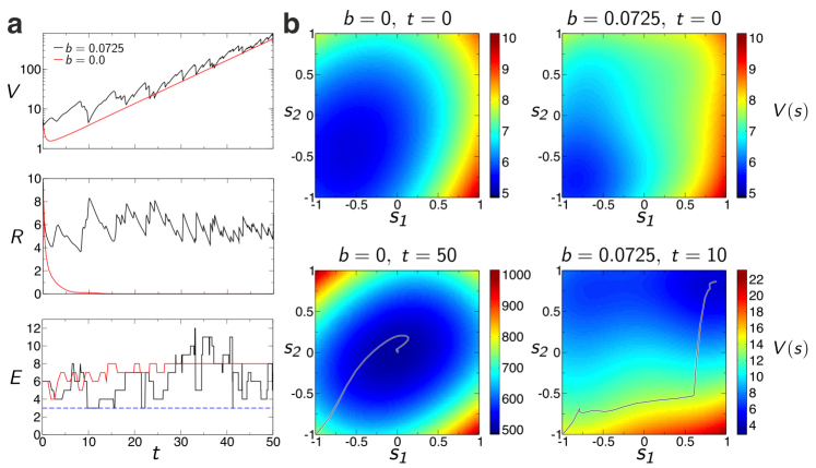
Figure 1: MaxSAT solver dynamics. The 3-MaxSAT formula used here has $N=10$, $M=80$ (clauses given in the Supplementary Table S1.) (a) The potential $V$, the radius $R=\sqrt{\sum_{i}s_{i}^{2}}$, and the number of unsatisfied clauses (energy) $E$ as function of analog time $t$ for the original dynamics corresponding to $b=0$ (red) and the modified dynamics with $b=0.0725$ (black). (b) Colormaps of the potential $V(\bm{s}(t),\bm{a}(t))$ in the plane $(s_{1},s_{2})$. At a given time instant $t$ we fix all values $s_{j}(t),j=3,\dots,N$ and $a_{m}(t),\forall m$ and change only $s_{1},s_{2}$ in the $[-1,1]\times[-1,1]$ plane, showing the instantaneous potential energy landscape $V$ in this plane. The curves indicate the projection of the trajectory onto $(s_{1},s_{2})$ up to the indicated time $t$. In $t=0$, $s_{1}=s_{2}=-1$. For $b=0$, the dynamics converges to $\bm{s}=0$, which is the centre of a deep well in the potential landscape. For $b=0.0725$, the centre is not a minimum anymore and at time $t=10$ the orthant with minimal energy $E_{min}=3$ is found (the solution), shown as a blue dotted line in the $E(t)$ figure.

There are several possibilities for such terms, here we focus on one version that works well in simulations:

$$V(\bm{s},\bm{a})=\sum_{m=1}^{M}a_{m}K_{m}(\bm{s})^{2}+b\alpha a\sum_{i=1}^{N}\cos^{2}\left(\frac{\pi}{2}s_{i}\right),$$ (4)

where $a$ is the average value of the auxiliary variables, $\alpha=M/N$ is the constraint density and $b$ is a constant factor tuning the strength of the last term to be always larger than the first, when chosen properly. The sum with the $\cos^{2}\left(\pi s_{i}/2\right)$ terms ensures the symmetric hat form, vanishing in the corners of ${\cal H}_{N}$. Note that the first term on the rhs of (4) is never larger than $aM$. We now have $V(\bm{0},\bm{a})=\left(2^{-2k}+b\right)aM$ and $b$ can be chosen such as to avoid the trapping phenomenon by the origin as described above, see also Fig.1b. To do that, we simply demand that the potential in the origin $V(\bm{0},\bm{a})$ keeps growing approximately at the same rate as the potentials in the corners of the hypercube, never getting smaller than the potential in the global minimum (the smallest potential value in the corners). Thus, as long as $V(\bm{0},\bm{a})\geq V(\bm{s^{\prime}},\bm{a})$, where $\bm{s^{\prime}}$ is some corner of the hypercube accessed by the dynamics, the dynamics will not get attracted by the origin of the hypercube. Since $V(\bm{s^{\prime}},\bm{a})\simeq aE(\bm{s^{\prime}})$, this implies that $b\geq\frac{1}{M}E(\bm{s^{\prime}})-2^{-2k}$, where $E(\bm{s^{\prime}})/M$ is the fraction of unsatisfied clauses in $\bm{s^{\prime}}$. Clearly, the $b$ value can be chosen arbitrarily large, however, if it is too large, then it forces the dynamics to keep running close to the surface of the hypercube, somewhat lowering its performance. In practice, an $E^{\prime}=E(\bm{s^{\prime}})$ is easily found by running a trajectory with a sufficiently large $b$ value for some short time, then resetting $b\geq\frac{E^{\prime}}{M}-2^{-2k}$. If chosen this way the search dynamics itself is not sensitive to this parameter $b$. The new dynamical system thus becomes:

$$\dot{s}_{i}=-\frac{\partial V}{\partial s_{i}}=\sum_{m=1}^{M}2a_{m}c_{mi}K_{mi}(\bm{s})K_{m}(\bm{s})+\frac{\pi}{2}b\alpha a\sin\left(\pi s_{i}\right)\,,\;\;\;\forall i=1,\ldots,N$$ (5)

$$\dot{a}_{m}=a_{m}K_{m}\,,\;\;\;\forall m=1,\ldots,m\;$$ (6)

where in Eq. 5 we used the notation $K_{mi}(\bm{s})=K_{m}(\bm{s})/(1-c_{mi}s_{i})$.

Fig. 1 illustrates the difference between the two dynamics (see also Fig. S1). While for $b=0$ (original system) the dynamics converges rapidly to $\bm{s}=\bm{0}$ (seen, e.g., by monitoring the radius $R^{2}=\sum_{i}s_{i}^{2}\to 0$), the modified system with a properly chosen $b>0$ continues the search. It finds an orthant with the minimum energy quite quickly (by $t=10$), but it does not halt there, it continues the dynamics and returns to this minimum repeatedly (e.g., around $t\approx 16,22,41$). Fig. 1b shows the potential energy function landscape $V(\bm{s},\bm{a})$ in the $(s_{1},s_{2})$ plane.

An energy-dependent escape rate

The escape rate is an invariant measure of the dynamics introduced for characterizing transiently chaotic systems PNAS_KT84 ; chaosbook . In a transiently chaotic system the asymptotic dynamics is not chaotic, but, for example, settles onto a simple attractor, or escapes to infinity (in open systems), however, the non-asymptotic dynamics is chaotic, usually governed by a chaotic repeller. It is well known that for hyperbolic, transiently chaotic dynamical systems the probability of a randomly started trajectory not converging to an attractor by time $t$ (i.e., not finding a SAT solution in our case) decreases exponentially in time: $p(t)\sim e^{-\kappa t}$, where $\kappa$ is the escape rate LaiTel11 ; PhysRep_TL08 ; PNAS_KT84 .

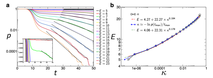
Figure 2: Energy dependent escape rate. (a) The $p(E,\,t)$ distributions for a hard, benchmark MaxSAT competition problem with $N=250$, $M=1000$ ($\alpha=4.0$) (source: benchmark14 ; benchmark16 , also the first row in table of Fig. 5). We obtain $E_{min}=5$ with our algorithm after running $\Gamma=2\times 10^{5}$ trajectories with $b=0.002375$. The escape rates are obtained from fitting $p\sim e^{-\kappa t}$ onto the last section of the distributions (black lines). (b) The energy $E$ vs the escape rate $\kappa$ using the values obtained from fitting shown in a) (black) and using the rough estimation for the escape rates $\kappa(E)\simeq-\ln(p(E,\,t_{max}))/t_{max}$ (blue). This estimation is convenient, as it is much easier to automate in the algorithm than the fitting procedure itself (see Methods). The dashed line curves show the fitting of Eq. (7). Both curves result in $E_{0}\in(4,5]$ thus predicting the global optimum $E^{pred}_{min}=5$.

The escape rate can also be interpreted as the inverse of the average lifetime $\tau$ of trajectories $\kappa=1/\tau$. For permanently chaotic systems, such as our MaxSAT solver, however, this definition does not work, as there is no simple asymptotic attractor in the dynamics and the system is closed. To be able to use a similar notion also for MaxSAT, we use a thresholding on the energy of the visited states. More precisely, we monitor the probability $p(E,\,t)$ that a trajectory has not yet found an orthant of energy smaller than $E$ by analog time $t$. Here $E$ acts as a parameter of the distribution. This can be measured by starting many trajectories from random initial conditions and monitoring the fraction of those that have not yet found a state with an energy less than $E$ by analog time $t$. In Fig.2a we show these distributions for different $E$ values for a MaxSAT problem. For large $E$, all trajectories almost immediately find orthants with fewer unsatisfied clauses, but for lower $E$ values the distributions decay exponentially. We call their decay rates energy-dependent escape rates $\kappa(E)$. Naturally, if an energy level does not exist in the system (e.g., for $E<E_{min}$), the escape rate for that energy level is meaningless (extrapolates to zero or a negative number). This suggests that the $\kappa(E)$ dependence could be used to predict where this minimum energy is reached. However, to capture this energy limit, it is more convenient to plot the $E(\kappa)$ function, instead (see Fig.2b). From extensive simulations, we observe a power-law behavior with an intercept $E_{0}$:

$$E=E_{0}+c\kappa^{\beta}\;.$$ (7)

Since $E_{0}$ is not an integer in general, we have $E_{min}=\lfloor E_{0}\rfloor+1$. This observation is at the basis of our method to predict the global energy minimum for MaxSAT.

Procedure for predicting the global minimum

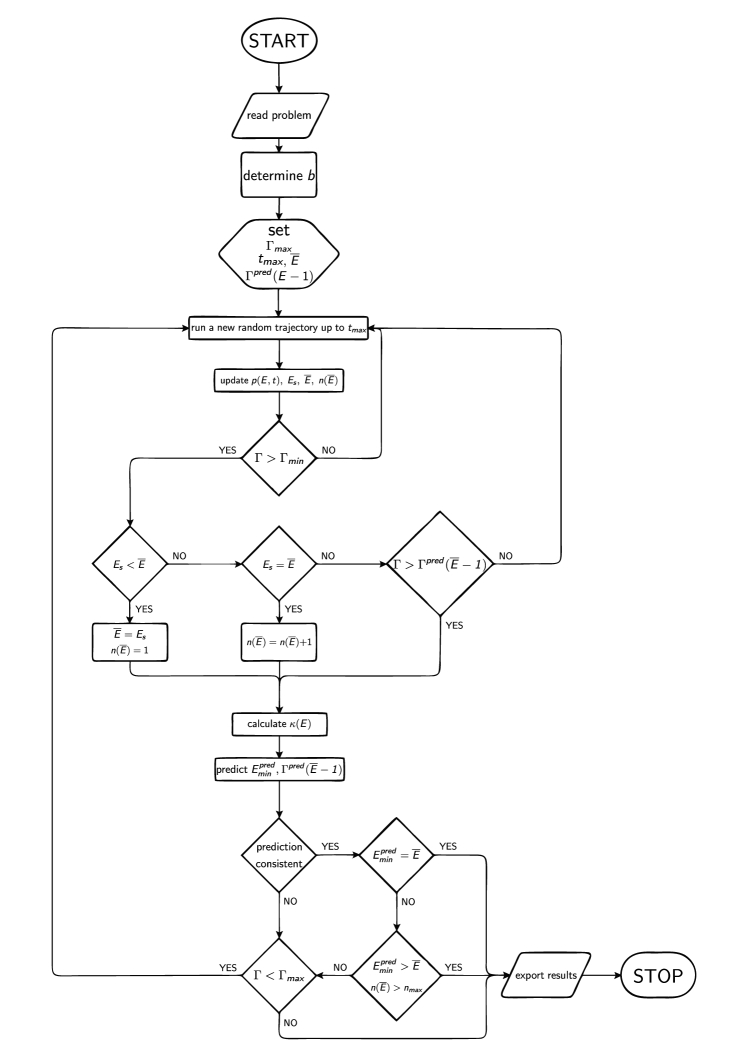
Figure S2: Flowchart of the dynamics described in detail in the Methods section.

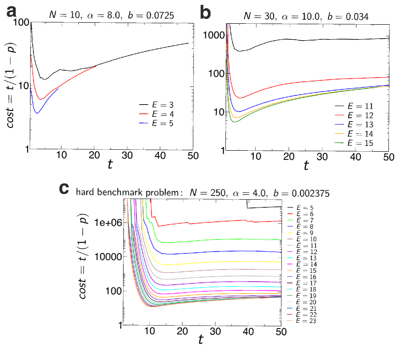
Figure S3: The cost of finding an energy level as function of time. If we run $\Gamma$ trajectories, each one up to time $t$, the total cost is proportional with $\Gamma t$. The number of times an energy level was found is equal to $\left(1-p(E,t)\right)\Gamma$, so we estimate the cost of finding a state with energy $E$ as $t/\left(1-p(E,t)\right)$. We plot this cost function for different energy levels for three different MaxSAT instances. (a) $N=10$, $\alpha=8.0$, $b=0.0725$, $E_{min}=3$. (b) $N=30$, $\alpha=10.0$, $b=0.034$, $E_{min}=11$. (c) The hard benchmark problem presented in detail in Figs. 2, 4 of the main text with $N=250$, $\alpha=4.0$, $b=0.002375$, $E_{min}=5$. The curves show a minimum at a relatively low $t$, indicating that it is much more efficient to run many short trajectories, than running a few for longer times. In case of random SAT instances with $N\leq 100$ we usually choose $t_{max}=25$. For larger instances such as the benchmark problem we used $t_{max}=50$ in our algorithm.

Here we describe the algorithm that also provides the halting criterion for the system (5-6) searching for solutions, with details of the computations presented in the Methods section along with an algorithm flowchart shown in Fig. S2. The exponentially decaying nature of the $p(E,\,t)$ distributions implies that sooner or later every trajectory will eventually visit the orthant with the lowest energy. Nevertheless, instead of leaving one trajectory to run for a very long time, it is more efficient to start many shorter trajectories from random initial conditions while tracking the lowest energy reached by each trajectory (see Fig. S3 and the Discussion section). This also generates good statistics for $p(E,\,t)$, and for obtaining the properties of the chaotic dynamics that are then exploited along with (7) to predict the value of the global minimum and to decide on the additional number of trajectories needed to find a lower energy state with high probability.

The basic step of the algorithm is to run a trajectory $\omega$ from a random initial condition up to a given time $t_{max}$ and record the lowest energy found by this particular trajectory, denoted by $E_{s}(\omega)$. Let $\Gamma$ denote the total number of trajectories run so far, ${\cal T}$ the set of these trajectories (thus $\Gamma=|{\cal T}|$), and $\overline{E}(\Gamma)=\min_{\omega\in{\cal T}}E_{s}(\omega)$ be the lowest energy found by all these trajectories. Using statistical methods and the relation between energy and escape rate $\kappa(E)$ (shown in (7)), the algorithm repeatedly predicts (as $\Gamma$ grows) the expected number of trajectories we need to run in total to find the lower energy value $\overline{E}-1$, i.e., $\Gamma^{pred}(\overline{E}-1)$ and the global minimum energy $E^{pred}_{min}$. We then monitor $E^{pred}_{min}$ for saturation and once the saturation criterion is reached, it outputs a decision $E^{dec}_{min}$, representing the final energy value predicted by the algorithm as the global minimum. If this energy value has actually already been attained (found at least one assignment for it), the algorithm outputs the corresponding assignment(s). If it did not attain it then it keeps running until finds such an assignment or reaches the preset maximum limit $\Gamma_{max}$ on the number of runs. In the latter case it outputs the lowest energy value attained and the corresponding assignment(s) and the consistency status of the predicted value. In the Methods section we provide the description of the algorithm.

Performance on random 3-MaxSAT problems

We first tested our algorithm and its prediction power on a large set (in total 4000) of random 3-MaxSAT problems with $N=30,50,100$ variables and constraint densities $\alpha=8,10$. (In 3-SAT the SAT-UNSAT transition is around $\alpha\simeq 4.267$ MezardZecchina ). We compare our results with the true minimum values ($E_{min}$) provided by the exact algorithm MaxSATZ MaxSatzAAAI ; MaxSatzJAIR .

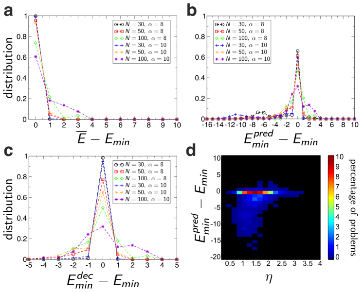
Figure 3: Algorithm statistics over random 3-MaxSAT problems. Distribution of differences between the real global minimum $E_{min}$ obtained with the exact algorithm MaxSatz and (a) the smallest energy found by the algorithm $\overline{E}$, (b) the predicted minimum value $E_{min}^{pred}$ and (c) the final decision of the algorithm $E_{min}^{dec}$ shown for problems with different $N$ and $\alpha$ values (see legends). (d) The percentage of instances indicated by color (see color bar) for different values of the error $E_{min}^{pred}-E_{min}$ and hardness $\eta$. Most instances are in the $E_{min}^{pred}-E_{min}=0$ row indicating correct prediction. Large errors occur mainly at smaller $\eta$ values, and are dominantly negative.

In Fig. 3 we compare the lowest energy found by the algorithm $\overline{E}$, the predicted minimum $E^{pred}_{min}$ and the final decision by the algorithm $E^{dec}_{min}$ with the true optimum $E_{min}$, by showing the distribution of differences across many random problem instances. We apply $t_{max}=25$ and limit the number of trajectories to $\Gamma_{max}=150\,000$, after which we stop the algorithm even if the prediction and the decision are not final. For that reason, it is expected that the performance of the algorithm decreases as $N$ increases, (e.g., at $N=100$), we would need to run more trajectories to obtain the same performance. Nevertheless, the results show that all three distributions have a large peak at $0$. Naturally, the most errors occur in the prediction phase, but many of these can be significantly reduced through simple decision rules (see Methods), because they occur most of the time in easy/small problems, where the statistics is insufficient (e.g., too few points since there are only few energy values).

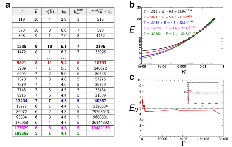
Figure 4: Performance of the algorithm illustrated on a hard benchmark problem. We use the same problem as in Fig. 2. (a) $\Gamma$ is the number of trajectories, $\overline{E}$ the lowest energy found until that point, $n(\overline{E})$ is the number of times this energy has been found, $E_{0}$ is the parameter obtained from fitting of Eq. (7), $E^{pred}_{min}$ and estimating $\Gamma^{pred}(\overline{E}-1)$. The algorithm estimates the escape rate and performs a prediction at each $\Gamma$ shown in the table and for the colored lines we show the fitting curves in (b). (c) The relevant parameter $E_{0}$ is shown as function of $\Gamma$. While it wildly fluctuates at the beginning when the statistics is small, it remains in the $E_{0}\in[4,5)$ interval, convincingly predicting $E^{pred}_{min}=5$ already after $\Gamma=7\,000$ up until the point that it finds this energy at $\Gamma=189\,562$. At this point it could be expected that we do not have a good estimate for $\kappa(5)$ because it has been found only once ($n(5)=1$), nevertheless the estimation $E^{pred}_{min}$ remains consistently the same, convincing our algorithm to accept $E^{dec}_{min}=5$ and stop.

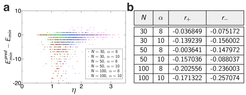
Figure S4: Correlation between the error of prediction and hardness of random 3-MaxSAT instances. (a) The difference between the predicted and real global minimum value as function of the hardness measure $\eta=-\log\kappa/\log N$, which is applicable for individual instances. We use different symbols and colors for instances with different $N$ and $\alpha$ (see legend). Large errors occur mainly in easy problems, at small $\eta$ values. (b) This is also shown by the negative values of the Pearson correlation coefficients obtained between the absolute value of errors and $\eta$, calculated separately for positive $(r_{+})$ and negative errors $(r_{-})$.

To show how the error in prediction depends on the hardness of problems, we studied the correlation between the error $E^{pred}_{min}-E_{min}$ and the hardness measure applicable to individual instances $\eta=-\ln\kappa/\ln N$ (for the origin and definition of this hardness measure see SciRep_ET12 ). In Fig. 3d we show the distribution of these values (also see Fig. S4). Interestingly, larger errors occur mainly at the easiest problems with $\eta<2$. Calculating the Pearson correlation coefficient between $|E^{pred}_{min}-E_{min}|$ and $\eta$ (excluding instances where the prediction is correct) we obtain a clear indication that often smaller $\eta$ (thus for easier problems) generates larger errors. Positive errors are much smaller and are shifted towards harder problems. There are somewhat more negative errors, which means that the algorithm consistently predicts a slightly lower energy value than the optimum, which is good, since this way we have an increased assurance that the algorithm has found the optimum state. In Fig. S4b we show the correlation coefficients calculated separately for problems with different $N$, $\alpha$ settings.

Performance evaluation on hard MaxSAT competition problems

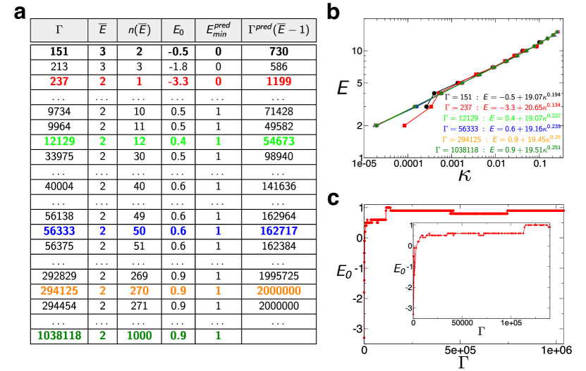
Figure S5: Performance of our algorithm on the 4-SAT problem HG-4SAT-V150-C1350 -24.cnf listed in the table of Fig. 5 of the main text. Similarly, to Fig. 4 of the main text in (a) we show the values of the relevant measures at each fitting performed. The fitting for each colored line is shown in (b). (c) The parameter $E_{0}$ that provides the final prediction of the global optimum is shown as function of $\Gamma$, the number of trajectories ran. In this case our predicition slightly underestimates the minimum, predicting 1. However, after the energy state 2 is found 1000 times we stop the search.

We next present the performance of our solver on very hard MaxSAT problems taken from competitions, listed on the site benchmark14 ; benchmark16 . For illustration purposes, here we focus on an extremely hard competition problem instance, called HG-3SAT-V250-C1000-1.cnf, which was reposted (for several years) with $N=250$ variables and $M=1000$ clauses, shown as problem No. 1 in the table of Fig. 5. This problem was also used in Fig. 2. No competition algorithm could solve this problem, or even predict the minimum energy value within the allotted time (30 mins). We ran our algorithm on a regular 2012 iMac 21.5, 3.1GHz, Intel Core i7 computer and it predicted the lowest energy of 5 (unsatisfied clauses), after 21min 24sec of running time and produced an assignment for it after 9.168h of running time. The minimum energy prediction was achieved already after $\Gamma=7000$ trajectories, whereas an assignment with this minimum energy took a total of $\Gamma=189\,562$ trajectories to run. The minimum energy assignment corresponding to $E^{dec}_{min}=5$ found by our algorithm is provided in the Supplementary Information section, Table S2. (The problem itself can be downloaded from the competition site benchmark16 ). We ran the complete and exact algorithm, MaxSatz MaxSatzAAAI ; MaxSatzJAIR for more than 5 weeks on this problem and the smallest energy it found was $E=9$! The details of how the algorithm performs are shown in Fig. 4. Similar figures for other hard problems such as for a 4-SAT problem and a spin-glass problem are shown in Figs. S5, S6.

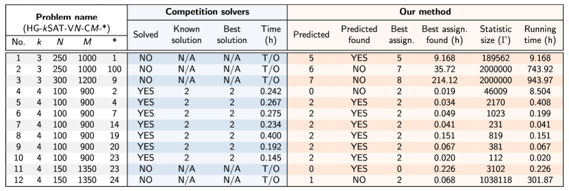
Figure 5: Algorithm performance on competition MaxSAT problems. The SAT instances can be downloaded from benchmark14 ; benchmark16 . The best solutions found by our algorithm are given in the SI.

The table of Fig. 5 shows the performance of the algorithm on several hard competition MaxSAT problems taken from the same source (notice, 9 out of 12 problems are 4-MaxSAT). Instances No. 1-3, 11, 12 were not solved by any competition solver, but our solver made a low energy prediction for all of them and for problems 1 and 11 it also did find an assignment corresponding to the predicted energy value. For No. 2, 3 and 12, it did not find a corresponding assignment, but, consistently finds an energy value that is only one higher (i.e., for 7 instead of 6, for 8 instead of 7 and 2 instead of 1). The reason for this is that the solver, by the nature of the fitting, sometimes predicts a lower energy value than the correct minimum one, as discussed previously. Note that the corresponding best assignment is found relatively early (even if the algorithm was run much longer, hoping to find a realization for the predicted value). Problems No. 4-10 were also solved by the competition solvers, achieving the best known solution (of 2 unsatisfied clauses in all cases), which was also found by our algorithm. In one instance, that of problem 4, it predicted an energy value of 0 (consistently with the observation of predicting lower values than than the minimum), which, of course it could not find, but it did find an assignment for the correct value of 2. In all these cases it found assignments faster than the competition solvers, often nearly ten times faster. In the Supplementary Information section we provide the minimum energy values and solution assignments for all the problems presented in Fig. 5.

Application to Ramsey numbers

Next we further demonstrate the ability of our analog algorithm to solve exceptionally hard MaxSAT problems. The problem of Ramsey numbers or Ramsey theory is a very active area in mathematics with applications to virtually every field of mathematics Bollobas ; RamseyTheory . Although it has several variants, in the standard, two-color Ramsey number problem we have to find the order for the smallest complete graph for which no matter how we color its edges with two colors (red and blue), we cannot avoid creating a monochromatic $m$-clique. The number of nodes for the smallest such complete graph is denoted by $R(m,m)$. The more popular formulation for $m=3$ is going back to Paul Erdős: minimum how many people $R(3,3)$ should we invite to a party to make sure that there are either 3 people who mutually all know each other or 3 people who mutually do not know each other? (In this case one edge color corresponds to people knowing each other and the other to not knowing each other). The proof that $R(3,3)=6$ is trivial. For $m=4$ the answer is $R(4,4)=18$ and it is harder to prove GG . The $m=5$ case is still open, only the bounds $43\leq R(5,5)\leq 48$ are known RamseyNumbersSurvey . The best lower bound of $43$ was first found in 1989 by Exoo Ex1 , and the upper bound was only recently reduced from 49 McKayRadz to 48 by Angeltveit and McKay R48 . Using various heuristic methods, including simulated annealing, tabu search and genetic algorithms, researchers have found in total 656 solutions (328 graphs and their complements) for the complete graph on 42 nodes McKayRadz . It has been conjectured by McKay and Radziszowski McKayRadz that there are no other solutions for $N=42$. Starting from these solutions they searched for a 5-clique-free coloring in 43 and as no solution was found, McKay, Radziszowski and Exoo made the strong conjecture that $R(5,5)=43$ McKayRadz . Other variants of Ramsey problems include specifying different clique orders for different colors and/or using more than two colors RamseyTheory .

Ramsey number problems are very challenging because the search space is huge: it grows as $2^{N(N-1)/2}=O(2^{N^{2}})$ with the order $N$ of the complete graph to be colored. To tackle Ramsey number problems with our algorithm, we first transform them into $k$-SAT: every edge $i$ ($i=1,\ldots,N(N-1)/2$) to be colored is represented by a Boolean variable $x_{i}$ (with $x_{i}\in\{0,1\}$, 1 = blue, 0 = red). A clique of size $m$ has $m(m-1)/2$ edges. We are satisfied with a coloring (a solution) when no $m$-clique is monochromatic, in other words, every $m$-clique with set of edges $\left\{i_{1},\ldots,i_{m(m-1)/2}\right\}$ must have both colors, expressed as the statement formed by the conjunction of the two clauses

$$\left(x_{i_{1}}\vee\ldots\vee x_{i_{m(m-1)/2}}\right)\wedge\left(\overline{x}_{i_{1}}\vee\ldots\vee\overline{x}_{i_{m(m-1)/2}}\right)$$ (8)

being true. This means that for every $m$-clique we have two clauses and thus there are a total of $2\binom{N}{m}$ clauses to satisfy. Since the number of clauses ($O(N^{m})$) for $m\geq 2$ grows faster in $N$ than the number of variables $N$, there will be a lowest $N$ value corresponding to UNSAT, which is the sought $R(m,m)$ Ramsey number. Thus, for $m=3$ we have a 3-SAT problem, for $m=4$ a 6-SAT problem and for $m=5$ a 10-SAT problem. For graphs with $N=42$ nodes the number of clauses is $1\,701\,336$ and the search space has over $2^{861}\simeq 1.5\times 10^{259}$ graphs! If we were to compute the familiar constraint density $\alpha$, it would be $\alpha=2\binom{42}{5}/(21\times 42)=1976$, indeed above the SAT/UNSAT transition point for random 10-SAT, which is estimated to be $\alpha_{s}{\big{|}}_{\mbox{\footnotesize 10-SAT}}\simeq 707$ 10SAT .

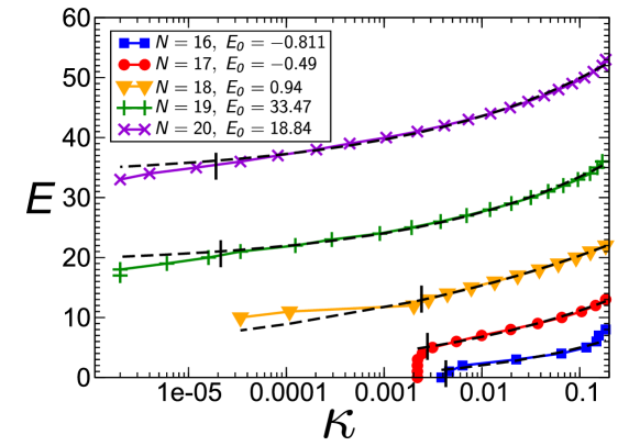
Figure 6: Finding the Ramsey number $R(4,4)$. The $E(\kappa)$ relationship for the 6-SAT problems corresponding to the $K_{N}$ complete graph colorings with two colors. $E_{0}$ is the extrapolated value based on the fit from Eq. (7) (dashed lines). The long vertical bars indicate the lower end of the fitting range. Note that for $N=16,17$, $E_{0}$ is a negative value indicating full colorability (the corresponding 6-SAT problem is fully satisfiable), whereas for $N\geq 18$, $E_{0}>0$, and thus the 6-SAT problem becomes MaxSAT.

Applying our algorithm for the $m=4$ Ramsey problem, we can easily find coloring solutions for $N\leq 17$, while for $N=18$ it predicts that there is no solution, indeed confirming that $R(4,4)=18$. This is seen from the plot of $E$ vs $\kappa$ in Fig 6. For $N\leq 17$ the smooth portion of the curve fitted by (7) suddenly cuts off, $\kappa$ being the same for all energy values lower than a threshold value, meaning that after reaching a state corresponding to the threshold energy level, the solution (i.e., $E=0$) is immediately found. This is simply due to the fact that the behavior (7) is a statistical average behavior characteristic of the chaotic trajectory, from the neighborhood of the chaotic repeller of the dynamics and away from the region in which the solution resides. However, once the trajectory enters the basin of attraction and nears the solution, the dynamics becomes simple, non-chaotic and runs into the solution, reflected by the sudden drop in energy. This is not due to statistical errors, because the curve remains consistent when plotting it using $10^{3},10^{4}$ or $10^{5}$ initial conditions (the figure shows $10^{5}$ initial conditions).

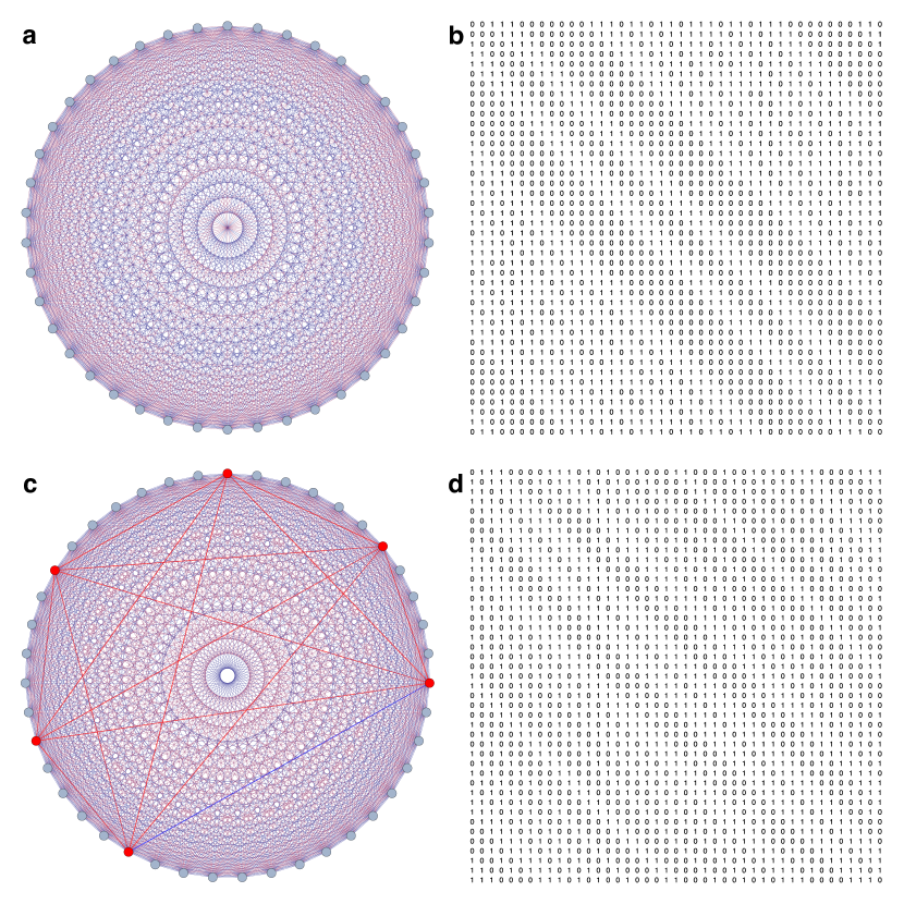
Figure 7: Colorings for the $R(5,5)$ Ramsey number problem. (a) A coloring of the complete graph on $N=42$ nodes that avoids monochromatic 5-cliques. (b) The adjacency matrix corresponding to the coloring in (a). (c) The best coloring of the complete graph on $N=43$ nodes containing only 2 monochromatic (red) 5-cliques, sitting on 6 nodes (highlighted with thicker edges). (d) The adjacency matrix corresponding to the coloring in (c).

Searching for the value of $R(5,5)$ one can relatively easily find coloring solutions without 5-cliques up to $N=35$ for which the number of variables is $595$ and the number of clauses $649\,264$, already huge for a 10-SAT problem for other types of SAT and MaxSAT solvers. To find solutions faster for $N\geq 36$, however, we employ a strategy based on circulant matrices Cyclic helping us find solutions (proper colorings) up to and including $N=42$ in a relatively short time (on the order of hours), which we describe next.

Kalbfleisch Cyclic argued that there should be coloring solutions of complete graphs for the Ramsey problem that can be described with a circulant form adjacency matrix (e.g., all red edges are 1-s, blue edges are 0-s in this matrix), or matrices that are close to such a circulant form. This was then later applied by many authors in improving bounds for Ramsey numbers and finding corresponding colorings. Although there is no formal proof of this statement, one expects this to be true also from the SAT formulation of the Ramsey problem. In the SAT formulation, the clauses have a very high degree of symmetry: all variables participate in the same way (8) in all the clauses, which run over all the possible $m$-cliques. This observation on symmetry can be exploited, allowing us to do part of the search in a much smaller space than the original space, where all the variables could in principle change independently from one another. More precisely, we first define a MaxSAT problem which has only $N-1$ variables (instead of the full $N(N-1)/2$) by choosing, e.g., those associated with the links of the first node: $x_{1}=a_{1,2},x_{2}=a_{1,3},\ldots,x_{N-1}=a_{1,N}$ as problem variables (here $a_{i,j}$ denotes the adjacency matrix) and defining the variables of the links of the other nodes by the circular permutation of this vector $\bm{x}$, to obtain a circulant matrix (e.g., $a_{2,3}=a_{1,2}$, $a_{i,j}=a_{i-1,j-1}$). Taking the MaxSAT form of the Ramsey problem we replace the variable of a link $a_{i,j}$ with $x_{j-i}$, thus reducing the number of independent variables from $N(N-1)/2$ to $N-1$. The number of clauses will also be reduced, because we can now eliminate the repeated ones. This way we obtain a much smaller MaxSAT problem, on which we apply our solver and starting from random initial conditions we search for low-energy states, which are relatively easily found. We save the $\bm{x}$ vectors (the Boolean values) corresponding to such low-energy circulant matrix states. For $N=42$ we have found circulant type matrices having only 6, 14, 20, 26 etc. monochromatic 5-cliques, indicating that they may already be close to a solution. After saving these circulant matrix states (with small number of monochromatic 5-cliques) we return to the original 10-SAT problem (with $N(N-1)/2$ variables, without the symmetry constraint), and start a new trajectory from the corner of the hypercube corresponding to the saved matrix state, but now without symmetry restriction. This places the trajectories relatively close to the solution and a proper coloring can be found in hours even for $N=42$, (see Fig. 7a, b, and Table S15 for an easily readable list of edge colorings), for which other heuristic algorithms take many days of computational time McKayRadz , even with the circulant matrix strategy. Applying the same strategy for $N=43$ we did not find any complete coloring solutions, however, we did find a coloring that creates only two (out of $962\,598$ possible) monochromatic 5-cliques, see Fig. 7c, d, and the specific coloring provided in the Supplementary Information Table S16. This adds further support to the conjecture that $R(5,5)=43$.

Discussion

In summary, here we presented a novel, continuous-time dynamical system approach to solve a quintessential discrete optimization problem, MaxSAT. The solver is based on a deterministic set of ordinary differential equations and a heuristic method that is used to predict the likelihood that the optimal solution has been found by analog time $t$. The prediction part of the algorithm uses the statistics of the ensemble of trajectories started from random initial conditions, by introducing the notion of energy-dependent escape rate and extrapolating this dependence to predict both the minimum energy value (lowest number of unsatisfied clauses) and the expected time needed by the algorithm to reach that value. The statistical analysis of the ensemble of trajectories presented here is very simple; it is quite possible that more sophisticated, extreme value statistical methods can be used to better predict minima values and time lengths. Due to its general character, the presented approach is generalizable to other optimization problems as well, to be presented in forthcoming publications.

Despite the fact that we are running our solver on digital computers (using a Runge-Kutta algorithm with adaptive step-size, 5th order Cash-Karp method for solving the ODEs) and not on an analog device, it still shows superior performance on very hard MaxSAT problems, compared to competition solvers. This is because analog dynamical systems represent an entirely novel family of solvers and search dynamics, and for this reason they behave differently and thus can perform better than existing algorithms on hard problems or certain classes of hard problems. Trying to solve large, but simple MaxSAT problems on digital computers with this method, however, would show a weaker performance than digital MaxSAT solvers, simply because evolving a large number of coupled ODEs on digital machines is costly. Direct hardware implementations, however, for example, via analog circuits are expected to run orders of magnitude faster than any state-of-the-art SAT solver run on the latest digital computers, as shown in Xunzhao . One reason for this is that in such analog circuits the von Neumann bottleneck is eliminated, with the circuit itself serving its own processor and memory, see Xunzhao for details. It is also important to note that the system (5-6) is not unique, other ODEs can be designed with similar or even better properties. This is useful, because the form given in (5-6) is not readily amenable to simple hardware implementations, due to the constantly growing auxiliary variable dynamics (all variables represent a physical characteristic such as a voltage or a current and thus they will have to have an upper limit value for a given device). However, the auxiliary variables do not need to grow always exponentially, there are other solver variants in which they only grow exponentially when needed, otherwise they can decay as well ModSystem , allowing for better hardware implementations.

To illustrate the effectiveness of our solver, as an application, we used it to find colorings in the famous two-color Ramsey problem and in particular for $R(5,5)$, which is still open. We have shown, that the two-color Ramsey problem avoiding monochromatic $m$-cliques can be translated into an $\frac{m(m-1)}{2}$-SAT problem and thus into a $10$-SAT problem for $m=5$. Note that most digital SAT solving algorithms focus on 3-SAT or 4-SAT problems, and usually are unable to handle directly the much harder $10$-SAT. Our solver when run on the corresponding $10$-SAT (or $10$-MaxSAT) was able to find colorings of the complete graph of order 42 avoiding monochromatic 5-cliques, and a coloring with only two (!) monochromatic 5-cliques on 6 nodes for the complete graph on 43 vertices (existing colorings in the literature for $N=43$ quote 500+ monochromatic 5-cliques), adding further support to the conjecture that $R(5,5)=43$.

Methods

1. Algorithm description

Here we give a simple, non-optimized variant of the algorithm (see flowchart in Fig. S2). Certainly, better implementations can be devised, for example with better fitting routines, however the description below is easier to follow and works well. Given a SAT problem, we first determine the $b$ parameter as described previously, then:

• Initially we set $\overline{E}=M$, $\Gamma_{min}$, $\Gamma_{max}\gg\Gamma_{min}$, $\Gamma^{pred}\left(\overline{E}-1\right)=\Gamma_{min}+1$ and $t_{max}$. Unless specified otherwise, in our simulations we used $\Gamma_{min}=100$, $\Gamma_{max}=2\times 10^{6}$, $t_{max}=50$.

• To initialize our statistics, we run $\Gamma_{min}$ trajectories up to $t_{max}$, each from a random initial condition. For every such trajectory $\omega$ we update the $p(E,\,t)$ distributions as function of the energies of the orthants visited by $\omega$. We record the lowest energy value found $\overline{E}(\Gamma_{min})$.

• Starting from $\Gamma=\Gamma_{min}+1$ and up to $\Gamma_{max}$, we continue running trajectories in the same way and for each one of them check:

  • if $E_{s}\leq\overline{E}$, set $\overline{E}\mathrel{\vbox{\hbox{\scriptsize.}\hbox{\scriptsize.}}}=\min(E_{s},\overline{E})$, update $p(E,\,t)$ and go to step 4.

  • if $\Gamma$ just reached $\Gamma^{pred}\left(\overline{E}-1\right)$, go to step 4.

  • if $\Gamma=\Gamma_{max}$, output “Maximum number of steps reached, increase $\Gamma_{max}$.”, output the lowest energy value found, the predicted $E^{pred}_{min}$ and the quality of fit for $E^{pred}_{min}$, then halt.

• Using the $p(E,\,t)$ distributions, estimate the escape rates $\kappa(E)$ as described in Methods section 2.

• The $\kappa(E)$ curve is extrapolated to the $E-1$ value obtaining $\kappa(E-1)$ and then using this we predict $\Gamma^{pred}\left(\overline{E}-1\right)$ (Methods section 3). Further extrapolating the $\kappa(E)$ curve to $\kappa=0$ we obtain $E^{pred}_{min}$ (see Methods section 4).

• We check the consistency of the prediction defined here as saturation of the predicted values. We call it consistent, if $E^{pred}_{min}$ has not changed during the last 5 predictions. If it is not consistent yet, we go to step 4 and continue running new trajectories. If the prediction is consistent, we check for the following halting conditions:

  • if $E^{pred}_{min}=\overline{E}(\Gamma)$ then we decide the global optimum has been found: $E^{dec}_{min}=E^{pred}_{min}=\overline{E}(\Gamma)$ and go to step 7.

  • if the fitting is consistently predicting $E^{pred}_{min}>\overline{E}(\Gamma)$ (usually it is very close, $\overline{E}(\Gamma)+1$) we check the number of trajectories that has attained states with $\overline{E}(\Gamma)$, i.e., $n(\overline{E})=\left[1-p(\overline{E}(\Gamma),\,t_{max})\right]\Gamma$. If it is large enough (e.g. $>100$), we decide to stop running new trajectories and set $E^{dec}_{min}=\overline{E}(\Gamma)$ and go to step 7.

  • if $E^{pred}_{min}<\overline{E}(\Gamma)$ then we most probably have not found the global optimum yet and we go to step 4.

  We added additional stopping conditions that can shorten the algorithm in case of easy problems, see Methods section 5, but these are not so relevant.

• The algorithm ends and outputs $E^{pred}_{min}$, $E^{dec}_{min}$, $\overline{E}$ values, the Boolean variables corresponding to the optimal state found, along with the quality of fit.

2. Estimation of the escape rates $\kappa(E)$

As seen in Fig. 2 and Fig. S1 the exponential decay of the $p(E,\,t)$ distribution settles in after a short transient period. Theoretically the escape rate can be obtained by fitting the exponential on that last part of the curves (Fig. 2a). However, while running the algorithm it would be difficult to automatically estimate the region where the exponential should be fitted. The simple approach that works well is to estimate the escape rates as $\kappa(E)\simeq-\ln(p(E,\,t_{max})/t_{max}$, which practically would correspond to the exponential behavior being valid on the whole $(0,t_{max})$ interval. Note, the $p(E,\,t)$ is a cumulative distribution with $p(E,\,0)=1$. Usually this estimation is very close to the fitted values (Fig. 2b), but notice that what matters here is the scaling behavior of the escape rates, and this is quite precisely obtained this way because it simply uses the scaling behavior of the $p(E,\,t_{max})$ values, instead of the fittings, which is sensitive to the chosen interval.

3. Predicting the number of trajectories needed to find a lower energy

After calculating the escape rates $\kappa(E)$ one can estimate the number of expected trajectories needed to find a lower energy value: $\Gamma^{pred}(\overline{E}-1)$ as described below. Clearly, $p(E,\,t_{max})$ is the probability that a trajectory has not reached the energy level $E$ up to time $t_{max}$. This means that $1-p(E,\,t_{max})$ is the probability that a trajectory did reach energy $E$, up to time $t_{max}$. Running $\Gamma$ trajectories, thus $n(\overline{E})=[1-p(E,t_{max})]\Gamma$ will give the expected number of trajectories that reached energy $E$. Thus, the expected number of trajectories we need to run in total to find the $\overline{E}-1$ energy value at least once is:

$$\Gamma^{pred}(\overline{E}-1)=\frac{1}{1-p(t_{max},\;\overline{E}-1)}\;.$$ (9)

However, no trajectory has reached energy $\overline{E}-1$ yet, and thus we don’t have $p(\overline{E}-1,\,t_{max})$. Instead, it is computed from $p(\overline{E}-1,\,t_{max})\simeq e^{-\kappa(\overline{E}-1)t_{max}}$, after extrapolating the $\kappa(E)$ curve to obtain $\kappa(\overline{E}-1)$.

4. Predicting the global optimum

When fitting the curve $E=E_{0}+a\kappa^{\beta}$ on our data points we used the Numerical Recipes implementation NumRec92 of the Levenberg-Marquardt non-linear curve fitting method Levenberg44 ; Marquardt63 . This implementation has some weaknesses, one could choose to use other implementations or other methods. Sometimes a 3-parameter fitting is too sensitive and does not give good results. Because we do not need a very precise value for $E_{0}$ (we just need to find the integer interval it falls into, because $E_{min}^{pred}=[E_{0}]+1$, $[.]$ meaning the integer part) we perform a series of fittings always fixing $E_{0}$ and leaving only 2 unknown parameters ($a,\beta$). For each $E_{0}=\overline{E},\overline{E}-0.1,\overline{E}-0.2,....$ we then perform a fitting and check the $\chi^{2}$ error. The fitting with minimal error is chosen as the final $E_{0}$ and final fitted curve.

5. Additional stopping conditions

There are cases usually for easy problems, when the fitting using the form (7) does not work well, but based on certain simple conditions we can trust that the global optimum has been found. For example:

• if there are not enough (e.g less than 5) data points in the $\kappa(E)$ curve fitted (this partly explains why the fitting does not give good prediction), but the lowest energy has already been found many times ($n(\overline{E})>n_{max}$, e.g. $n_{max}=1000$). This happens for very easy problems.

• The fitting is consistently predicting another $E^{pred}_{min}\neq\overline{E}$, but $n(\overline{E})$ is very large and $\Gamma>\Gamma^{pred}(\overline{E}-1)$, so according to the dynamics, it seems a lower energy should have been found already.

In such cases we exit the algorithm (step 7) with the decision: $\overline{E}\neq E^{pred}_{min},E^{dec}_{min}=\overline{E}$.

Author Contributions

The authors designed the methods and algorithm together, contributed analysis and tools equally. Both ZT and MER wrote and reviewed the manuscript.

Additional Information

Competing financial interests The authors declare no competing financial interests.

Supplementary Information

Supplementary Figures

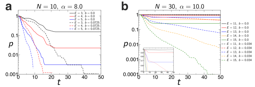
Figure S1: The $p(E,t)$ distribution of transient times compared between the SAT-solver algorithm presented in NatPhys_ET11 and the new max-SAT solver dynamics. $p(E,t)$ is the probability that up to time $t$ a trajectory has not yet visited an orthant with energy smaller than E. As shown for two max-SAT instances (a) $N=10$, $\alpha=8.0$, $b=0.0725$, $E_{min}=3$. (b) $N=30$, $\alpha=10.0$, $b=0.034$, $E_{min}=11$, when $b=0$ (the original analog SAT solver dynamics) the exponential decay of the distribution stops at relatively small $t$ indicating that many trajectories have been trapped at $\bm{s}=0$. When $b>0$ the distribution is much steeper and the trapping phenomenon does not occur.

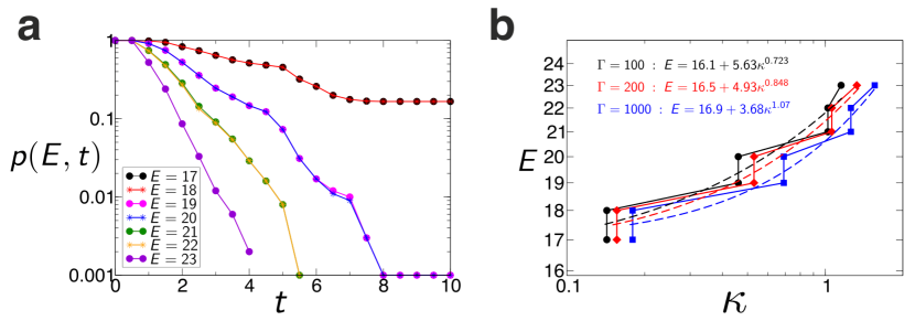
Figure S6: Predicting the global optimum in a spin-glass hard benchmark problem. $k=2$, $N=27$, $M=162$, $E_{min}=17$, $b=0.042438$ (the problem instance t3pm3-5555.spn.cnf can be downloaded from benchmark14 ). Note, Max-2-SAT is also NP-hard, unlike 2-SAT, which is in P. (a) The $p(E,t)$ distributions after running $\Gamma=1000$ trajectories. Because of the special structure of the spin-glass problem pairs of consecutive energy levels show the same distributions (a single spin-flip can change the energy only in units of 2). (b) The energy $E$ as function of the estimated $\kappa(E)$ values after running $\Gamma=100,200,1000$ trajectories (see legend). The fitted curves are shown with dashed lines. $E_{0}\in[16,17)$ indicating a correct prediction already after $\Gamma=100$ trajectories. This is an easy problem for our algorithm and $E_{min}=17$ is found 79 times by the first $\Gamma=100$ trajectories.

Supplementary tables and data

Table S1: The 3-SAT problem shown in Figure 1 of the main text. We have $N=10$ variables and $M=80$ clauses (constraints) in conjunctive normal form. Each clause is shown in parenthesis as the series of 3 variables or their negation (indicated by negative sign). For example, the first triple in parantheses indicates the clause/constraint: ($x_{5}$ OR (NOT $x_{8}$) OR $x_{9}$).

(5,-8,9)(-1,-3,-7)(9,4,-8)(-1,-9,4)(7,2,3)(9,5,4)(8,9,-3)(10,-5,9)(9,7,8)(3,1,6) (7,10,3)
(-5,10,-3)(-7,6,4)(-8,1,-10)(-1,-2,3)(-9,-2,-3)(5,7,8)(-5,-3,4)(9,-2,1)(-3,-1,-7)(10,5,4)
(-7,-10,-4)(-9,-10,3)(2,-1,10)(-5,-10,-7)(-9,6,8)(-9,-4,-8)(-5,-3,-8)(-9,3,-7)(-6,2,5)
(-2,1,-8)(1,6,9)(5,-9,2)(10,-1,7)(5,-1,-3)(6,-7,2)(8,-5,7)(-8,-7,-3)(4,-7,3)(4,-9,2)(1,6,-7)
(-9,-2,5)(10,-4,-5)(4,-2,-9)(-7,2,1)(4,2,-8)(-2,-10,-5)(6,-3,7)(-1,-3,7)(-1,6,4)(-9,-4,3)
(-4,10,-5)(9,6,-2)(-8,-2,5)(2,-1,3)(-6,-4,10)(7,-5,2)(7,3,-5)(-7,9,-6)(-4,6,2)(-6,9,-5)
(-10,-1,2)(5,-8,-7)(8,7,-2)(-8,-2,1)(6,1,-8)(8,5,-2)(-8,3,6)(10,2,-3)(9,-7,2)(-6,10,2)
(1,-3,4)(6,2,-8)(9,2,10)(2,5,-1)(-1,8,4)(-3,1,-4)(-10,9,-7)(-4,-5,-9)(-6,-7,10)

The problem instances with the solutions presented in Tables S2-S13 below can all be downloaded from benchmark14 , benchmark16 .

Table S2: The optimal solution (list of Boolean variables corresponding to the optimal state found) found for the HG-3SAT-V250-C1000-1.cnf MaxSAT competition problem: $E_{min}=5$.

0 1 1 1 1 0 1 1 0 1 1 1 1 1 0 0 0 1 0 0 0 0 0 1 1 1 1 1 1 1 0 1 1 0 0 0 0 1 1 0 0 1 0 0 0 0 0 1 1 1

0 0 1 1 1 0 1 1 1 1 1 0 0 1 1 0 0 0 0 0 1 0 0 0 0 1 1 0 1 0 1 0 0 0 1 1 1 0 0 1 0 0 0 1 1 1 1 0 1 0

0 0 1 0 0 0 0 0 0 0 0 0 0 0 0 1 1 0 0 1 0 0 1 1 0 1 0 0 0 0 1 1 1 0 0 0 1 0 0 1 0 1 1 0 0 0 1 1 1 0

0 0 1 0 0 1 1 1 0 1 1 0 1 1 1 0 0 0 1 0 0 0 0 1 0 1 1 1 0 1 1 1 1 1 0 1 0 1 0 0 0 0 1 0 0 1 1 0 0 1

0 0 1 1 1 0 0 1 1 1 1 1 0 0 1 1 0 0 1 0 1 0 1 0 1 0 0 0 0 0 1 0 1 0 1 1 0 0 1 0 0 0 1 0 1 0 1 0 0 1

Table S3: HG-3SAT-V250-M1000-100.cnf optimal solution found: $E_{min}=7$.

1 1 1 0 1 1 1 0 0 1 0 1 0 1 1 1 1 0 0 0 1 0 0 1 0 0 1 1 1 1 1 0 1 1 1 1 0 0 1 1 1 1 1 1 0 0 1 0 1 0

0 0 1 0 0 1 0 1 1 1 0 1 0 0 1 1 1 1 0 1 1 0 0 0 1 1 1 1 1 1 1 0 0 0 1 0 1 1 1 1 1 0 1 1 0 0 0 0 1 0

1 0 1 1 0 0 0 1 1 0 1 0 0 0 1 0 1 0 0 0 1 1 1 1 0 0 0 0 0 0 1 0 1 0 1 0 0 0 1 0 1 0 0 0 1 0 0 1 0 1

1 0 0 1 0 1 1 0 0 1 0 1 0 1 1 1 1 1 1 1 1 0 0 0 0 1 0 0 1 0 1 1 1 0 0 0 0 1 0 1 1 0 0 0 1 1 0 1 1 0

0 0 1 1 0 0 1 0 1 0 0 0 1 1 1 1 1 0 0 0 0 1 1 1 1 0 1 0 0 0 0 1 1 0 0 0 1 1 1 0 0 0 0 0 0 1 1 0 1 1

Table S4: HG-3SAT-V300-M1200-9.cnf optimal solution found: $E_{min}=8$.

1 1 1 1 1 0 1 1 0 0 1 0 0 1 0 0 1 1 0 1 1 1 1 0 1 0 0 0 0 0 1 0 0 0 0 0 1 1 1 1 0 1 1 0 1 1 1 0 1 0 0

0 1 1 0 1 1 0 0 1 0 1 0 1 1 1 0 0 1 1 0 0 1 0 1 0 0 0 1 0 1 0 1 1 0 0 0 1 0 0 1 0 0 1 1 1 1 1 0 1 1 0

0 1 1 1 1 1 1 1 1 1 0 0 1 0 1 0 0 0 0 0 0 1 0 0 1 1 1 0 1 0 0 1 1 0 0 0 0 0 1 1 0 1 0 0 1 1 1 1 0 1 1

0 1 1 1 0 0 1 0 1 0 0 0 0 0 1 0 0 0 1 1 0 1 1 1 0 0 0 1 1 1 1 1 0 0 0 0 0 0 0 0 0 1 0 1 1 0 0 0 1 0 1

0 1 1 1 0 1 1 0 1 1 0 1 0 1 1 1 1 0 1 1 1 0 0 0 1 1 0 1 0 1 1 0 1 0 0 1 1 0 1 0 1 1 0 0 0 0 0 1 1 0 1

1 1 0 0 1 0 0 1 0 0 0 1 1 1 1 0 0 0 0 0 0 0 1 0 1 0 1 0 1 1 0 0 0 1 0 1 1 1 1 0 0 1 1 1 1

Table S5: HG-4SAT-V100-M900-2.cnf optimal solution found: $E_{min}=2$.

1 1 0 1 1 1 0 1 1 1 1 1 1 0 1 0 1 0 0 0 0 0 1 1 1 1 0 0 1 0 0 1 0 0 1 1 1 0 1 1 0 0 0 0 0 1 1 1 0 0 1

0 1 1 0 1 1 0 1 1 1 0 0 0 0 0 0 1 1 1 0 0 0 1 0 0 1 0 1 0 1 0 1 1 1 0 0 0 0 1 1 1 0 1 1 0 0 1 0 1

Table S6: HG-4SAT-V100-M900-4.cnf optimal solution found: $E_{min}=2$.

0 0 1 1 1 1 0 0 1 1 0 0 0 0 0 0 0 1 0 0 1 1 1 0 1 1 0 1 1 0 0 1 0 1 1 1 0 0 1 1 0 1 0 1 0 1 1 0 1 1 1

0 0 1 0 0 1 0 1 0 0 0 0 0 0 1 0 0 1 1 0 1 0 0 0 1 1 1 0 1 0 1 0 0 1 0 0 1 1 1 0 0 0 0 1 1 0 0 0 0

Table S7: HG-4SAT-V100-M900-7.cnf optimal solution found: $E_{min}=2$.

0 1 1 1 1 0 0 0 1 0 1 0 1 0 0 0 0 1 1 1 0 1 0 1 0 1 1 1 0 0 0 0 1 0 1 0 1 1 0 0 0 0 1 0 1 0 0 1 1 0 1

1 1 1 0 1 1 0 0 1 1 1 0 1 1 0 1 0 1 1 0 0 1 1 0 1 1 1 1 0 1 0 1 1 0 1 1 0 0 1 1 1 1 1 1 1 0 0 0 1

Table S8: HG-4SAT-V100-M900-14.cnf optimal solution found: $E_{min}=2$.

0 0 1 0 0 0 1 1 1 1 1 1 1 1 0 0 1 0 0 0 1 0 1 1 0 0 0 1 1 1 0 1 1 0 1 0 0 1 0 0 1 0 0 1 1 1 1 0 0 0 1

1 0 0 1 0 1 0 0 0 0 0 0 0 0 1 1 0 0 0 0 1 1 1 0 1 1 1 0 1 1 0 0 0 0 1 1 0 0 0 0 1 1 1 0 0 1 1 1 1

Table S9: HG-4SAT-V100-M900-19.cnf optimal solution found: $E_{min}=2$.

0 1 1 1 0 1 0 0 1 1 1 0 0 0 0 0 1 1 1 1 1 0 1 0 1 0 0 1 0 0 0 1 0 0 0 0 0 0 1 0 1 1 1 1 1 0 1 1 1 0 1

1 1 1 1 1 1 1 1 1 1 0 0 0 0 1 0 1 1 1 0 0 1 0 1 1 1 1 1 0 0 0 0 0 1 0 1 1 0 0 0 1 0 1 1 1 0 0 1 1

Table S10: HG-4SAT-V100-M900-20.cnf optimal solution found: $E_{min}=2$.

1 0 0 1 0 1 0 0 0 0 0 0 0 0 1 0 1 1 0 0 1 1 1 1 0 1 0 1 1 1 0 1 1 0 1 0 1 1 0 0 1 1 0 0 0 0 1 1 1 0 0 1

1 0 1 1 1 1 0 1 1 1 1 1 1 1 1 0 0 0 1 1 0 1 0 1 0 0 0 0 1 1 1 0 0 0 1 0 0 1 1 1 1 1 0 0 0 1 0 0

Table S11: HG-4SAT-V100-M900-23.cnf optimal solution found: $E_{min}=2$.

0 0 0 0 1 0 1 0 1 0 0 0 0 1 0 1 1 0 0 0 0 1 0 1 1 0 1 0 1 0 1 0 1 0 1 1 0 1 0 0 0 1 1 0 0 1 1 0 0 0 1 1

1 0 1 0 1 0 1 1 1 0 1 0 1 0 1 0 1 0 1 1 0 0 0 1 0 0 1 1 1 0 1 1 1 1 0 0 0 0 0 0 1 0 1 0 0 0 0 1

Table S12: HG-4SAT-V150-M1350-23.cnf optimal solution found: $E_{min}=0$.

0 1 1 0 0 0 0 1 1 0 1 1 1 0 0 0 0 1 1 0 1 1 0 1 1 1 0 0 1 1 1 0 1 0 1 0 0 1 0 0 0 0 0 0 1 0 0 1 0 1 0 1 1

0 1 0 0 0 1 0 1 0 1 1 0 0 1 1 0 0 1 0 0 0 0 0 1 1 1 0 1 0 1 0 1 1 0 1 1 1 1 0 1 1 0 0 1 0 1 1 1 1 1 0 0 0

1 1 0 1 0 1 1 1 1 1 1 0 1 1 1 0 0 0 0 0 0 1 0 1 0 1 0 1 1 0 1 0 0 0 0 1 1 1 1 0 0 1 1 0

Table S13: HG-4SAT-V150-M1350-24.cnf optimal solution found: $E_{min}=2$.

0 0 1 0 1 0 1 0 0 0 0 1 1 1 0 0 0 1 0 1 0 0 1 1 1 0 0 0 0 1 1 0 1 1 1 1 0 1 1 0 1 0 0 0 1 0 0 0 0 1 0 0

0 0 0 0 1 0 0 0 0 1 0 0 0 0 1 0 1 1 1 1 1 0 1 1 0 1 0 0 1 0 1 0 0 0 1 1 0 0 1 0 1 0 1 0 1 1 1 1 1 1 1 1

1 0 1 0 0 1 1 1 1 1 1 0 0 1 0 1 1 1 0 1 0 1 0 0 0 0 0 1 1 1 0 1 1 0 1 1 0 0 0 1 0 0 0 1 0 0

Table S14: Spin-glass problem t3pm3-5555.spn presented in Fig S6. Optimal solution found: $E_{min}=17$.

0 0 0 1 0 1 1 0 1 1 0 1 1 1 0 0 1 0 0 1 1 1 1 1 0 0 0

Table S15: The matrix shown in Fig. 7b of the main text that gives a complete Ramsey coloring of a complete graph on 42 nodes. There are no monochromatic 5-cliques ($E_{min}=0$).

0 0 1 1 1 0 0 0 0 0 0 0 1 1 1 0 1 1 0 1 1 0 1 1 1 0 1 1 0 1 1 1 0 0 0 0 0 0 0 1 1 0
0 0 0 1 1 1 0 0 0 0 0 0 0 1 1 1 0 1 1 0 1 1 1 1 1 1 0 1 1 0 1 1 1 0 0 0 0 0 0 0 1 1
1 0 0 0 1 1 1 0 0 0 0 0 0 0 1 1 1 0 1 1 0 1 1 1 0 1 1 0 1 1 0 1 1 1 0 0 0 0 0 0 0 1
1 1 0 0 0 1 1 1 0 0 0 0 0 0 0 1 1 1 0 1 1 0 1 1 0 0 1 1 0 1 1 0 1 1 1 0 0 0 1 0 0 0
1 1 1 0 0 0 1 1 1 0 0 0 0 0 0 0 1 1 1 0 1 1 0 1 1 0 0 1 1 0 1 1 0 1 1 1 0 0 0 0 0 0
0 1 1 1 0 0 0 1 1 1 0 0 0 0 0 0 0 1 1 1 0 1 1 0 1 1 1 1 1 1 0 1 1 0 1 1 1 0 0 0 0 0
0 0 1 1 1 0 0 0 1 1 1 0 0 0 0 0 0 0 1 1 1 0 1 1 0 1 1 1 1 1 1 0 1 1 0 1 1 1 0 0 0 0
0 0 0 1 1 1 0 0 0 1 1 1 0 0 0 0 0 0 0 1 1 1 0 1 1 0 1 1 0 0 1 1 0 1 1 0 1 1 1 0 0 0
0 0 0 0 1 1 1 0 0 0 1 1 1 0 0 0 0 0 0 0 1 1 1 0 1 1 0 1 1 0 0 1 1 0 1 1 0 1 1 1 0 0
0 0 0 0 0 1 1 1 0 0 0 1 1 1 0 0 0 0 0 0 0 1 1 1 0 1 1 0 1 1 0 1 0 1 0 1 1 0 1 1 1 0
0 0 0 0 0 0 1 1 1 0 0 0 1 1 1 0 0 0 0 0 0 0 1 1 1 0 1 1 0 1 1 0 1 1 1 0 1 1 0 1 1 1
0 0 0 0 0 0 0 1 1 1 0 0 0 1 1 1 0 0 0 0 0 0 0 1 1 1 0 1 1 0 1 1 0 0 1 1 0 1 1 0 1 1
1 0 0 0 0 0 0 0 1 1 1 0 0 0 1 1 1 0 0 0 0 0 0 0 1 1 1 0 1 1 0 1 1 0 0 1 1 0 1 1 0 1
1 1 0 0 0 0 0 0 0 1 1 1 0 0 0 1 1 1 0 0 0 0 0 0 0 1 1 1 0 1 1 0 1 1 0 1 1 1 0 1 1 0
1 1 1 0 0 0 0 0 0 0 1 1 1 0 0 0 1 1 1 0 0 0 0 0 0 0 1 1 1 0 1 1 0 1 1 1 1 1 1 0 1 1
0 1 1 1 0 0 0 0 0 0 0 1 1 1 0 0 0 1 1 1 0 0 0 0 0 0 1 1 1 1 0 1 1 0 1 1 1 0 1 1 0 1
1 0 1 1 1 0 0 0 0 0 0 0 1 1 1 0 0 0 1 1 1 0 0 0 0 0 0 0 1 1 1 0 1 1 0 1 1 0 0 1 1 0
1 1 0 1 1 1 0 0 0 0 0 0 0 1 1 1 0 0 0 1 1 1 0 0 0 0 0 0 0 1 1 1 0 1 1 0 1 1 0 0 1 1
0 1 1 0 1 1 1 0 0 0 0 0 0 0 1 1 1 0 0 0 1 1 1 0 0 0 0 0 0 0 1 1 1 0 1 1 0 1 1 1 1 1
1 0 1 1 0 1 1 1 0 0 0 0 0 0 0 1 1 1 0 0 0 1 1 1 0 0 0 0 0 0 0 1 1 1 0 1 1 0 1 1 1 1
1 1 0 1 1 0 1 1 1 0 0 0 0 0 0 0 1 1 1 0 0 0 1 1 1 0 0 0 0 0 0 0 1 1 1 0 1 1 0 1 1 0
0 1 1 0 1 1 0 1 1 1 0 0 0 0 0 0 0 1 1 1 0 0 0 1 1 1 0 0 0 0 0 0 0 1 1 1 0 1 1 0 1 1
1 1 1 1 0 1 1 0 1 1 1 0 0 0 0 0 0 0 1 1 1 0 0 0 1 1 1 0 0 0 0 0 0 0 1 1 1 0 1 1 0 1
1 1 1 1 1 0 1 1 0 1 1 1 0 0 0 0 0 0 0 1 1 1 0 0 0 1 1 1 0 0 0 0 0 0 0 1 1 1 0 1 1 0
1 1 0 0 1 1 0 1 1 0 1 1 1 0 0 0 0 0 0 0 1 1 1 0 0 0 1 1 1 0 0 0 0 0 0 0 1 1 1 0 1 1
0 1 1 0 0 1 1 0 1 1 0 1 1 1 0 0 0 0 0 0 0 1 1 1 0 0 0 1 1 1 0 0 0 0 0 0 0 1 1 1 0 1
1 0 1 1 0 1 1 1 0 1 1 0 1 1 1 1 0 0 0 0 0 0 1 1 1 0 0 0 1 1 1 0 0 0 0 0 0 0 1 1 1 0
1 1 0 1 1 1 1 1 1 0 1 1 0 1 1 1 0 0 0 0 0 0 0 1 1 1 0 0 0 1 1 1 0 0 0 0 0 0 0 1 1 1
0 1 1 0 1 1 1 0 1 1 0 1 1 0 1 1 1 0 0 0 0 0 0 0 1 1 1 0 0 0 1 1 1 0 0 0 0 0 0 0 1 1
1 0 1 1 0 1 1 0 0 1 1 0 1 1 0 1 1 1 0 0 0 0 0 0 0 1 1 1 0 0 0 1 1 1 0 0 0 0 0 0 0 1
1 1 0 1 1 0 1 1 0 0 1 1 0 1 1 0 1 1 1 0 0 0 0 0 0 0 1 1 1 0 0 0 1 1 1 0 0 0 0 0 0 0
1 1 1 0 1 1 0 1 1 1 0 1 1 0 1 1 0 1 1 1 0 0 0 0 0 0 0 1 1 1 0 0 0 1 1 1 0 0 0 0 0 0
0 1 1 1 0 1 1 0 1 0 1 0 1 1 0 1 1 0 1 1 1 0 0 0 0 0 0 0 1 1 1 0 0 0 1 1 1 0 0 0 0 0
0 0 1 1 1 0 1 1 0 1 1 0 0 1 1 0 1 1 0 1 1 1 0 0 0 0 0 0 0 1 1 1 0 0 0 1 1 1 0 0 0 0
0 0 0 1 1 1 0 1 1 0 1 1 0 0 1 1 0 1 1 0 1 1 1 0 0 0 0 0 0 0 1 1 1 0 0 0 1 1 1 0 0 0
0 0 0 0 1 1 1 0 1 1 0 1 1 1 1 1 1 0 1 1 0 1 1 1 0 0 0 0 0 0 0 1 1 1 0 0 0 1 1 1 0 0
0 0 0 0 0 1 1 1 0 1 1 0 1 1 1 1 1 1 0 1 1 0 1 1 1 0 0 0 0 0 0 0 1 1 1 0 0 0 1 1 1 0
0 0 0 0 0 0 1 1 1 0 1 1 0 1 1 0 0 1 1 0 1 1 0 1 1 1 0 0 0 0 0 0 0 1 1 1 0 0 0 1 1 1
0 0 0 1 0 0 0 1 1 1 0 1 1 0 1 1 0 0 1 1 0 1 1 0 1 1 1 0 0 0 0 0 0 0 1 1 1 0 0 0 1 1
1 0 0 0 0 0 0 0 1 1 1 0 1 1 0 1 1 0 1 1 1 0 1 1 0 1 1 1 0 0 0 0 0 0 0 1 1 1 0 0 0 1
1 1 0 0 0 0 0 0 0 1 1 1 0 1 1 0 1 1 1 1 1 1 0 1 1 0 1 1 1 0 0 0 0 0 0 0 1 1 1 0 0 0
0 1 1 0 0 0 0 0 0 0 1 1 1 0 1 1 0 1 1 1 0 1 1 0 1 1 0 1 1 1 0 0 0 0 0 0 0 1 1 1 0 0

Table S16: The coloring matrix shown in Fig. 7d with only 2 monochromatic 5-cliques sitting on 6 vertices of a complete graph with 43 nodes ($E_{min}=2$).

0 1 1 1 0 0 0 0 1 1 1 0 1 0 1 0 0 1 0 0 0 1 1 0 0 0 1 0 0 1 0 1 0 1 1 1 0 0 0 0 1 1 1
1 0 1 1 1 0 0 1 0 1 1 1 0 1 0 1 0 0 1 0 0 0 1 1 0 0 0 1 0 0 1 0 1 0 1 1 1 0 0 0 0 1 1
1 1 0 1 1 1 0 0 1 0 1 1 1 0 1 0 1 0 0 1 0 0 0 1 1 0 0 0 1 0 0 1 0 1 0 1 1 1 0 1 0 0 1
1 1 1 0 1 1 1 0 0 1 0 1 1 1 0 1 0 1 0 0 1 0 0 0 1 1 0 0 0 1 0 0 1 0 1 0 1 1 1 0 1 0 0
0 1 1 1 0 1 1 1 0 0 0 0 1 1 1 0 1 0 1 0 0 1 0 0 0 1 1 0 0 0 1 0 0 1 0 1 0 1 1 1 0 1 0
0 0 1 1 1 0 1 1 1 0 0 0 0 1 1 1 0 1 0 1 0 0 1 0 0 0 1 1 0 0 0 1 0 0 1 0 1 0 1 1 1 0 0
0 0 0 1 1 1 0 1 1 1 0 0 0 0 1 1 1 0 1 0 1 0 0 1 0 0 0 1 1 0 0 0 1 0 0 1 0 1 0 1 1 1 0
0 1 0 0 1 1 1 0 1 1 1 0 0 1 0 1 1 1 0 1 0 1 0 0 1 0 0 0 1 1 0 0 0 1 0 0 1 0 1 0 1 1 1
1 0 1 0 0 1 1 1 0 1 1 1 0 0 1 0 1 1 1 0 1 0 1 0 0 1 0 0 0 1 1 0 0 0 1 0 0 1 0 1 0 1 1
1 1 0 1 0 0 1 1 1 0 1 1 1 0 0 1 0 1 1 1 0 1 0 1 0 0 1 0 0 0 1 1 0 0 0 1 0 0 1 0 1 0 1
1 1 1 0 0 0 0 1 1 1 0 1 1 1 0 0 0 0 1 1 1 0 1 0 1 0 0 1 0 0 0 1 1 0 0 0 1 0 0 1 0 1 0
0 1 1 1 0 0 0 0 1 1 1 0 1 1 1 0 0 0 0 1 1 1 0 1 0 1 0 0 1 0 0 0 1 1 0 0 0 1 0 0 1 0 1
1 0 1 1 1 0 0 0 0 1 1 1 0 1 1 1 0 0 1 0 1 1 1 0 1 0 1 0 0 1 0 0 0 1 1 0 0 0 1 0 0 1 0
0 1 0 1 1 1 0 1 0 0 1 1 1 0 1 1 1 0 0 1 0 1 1 1 0 1 0 1 0 0 1 0 0 0 1 1 0 0 0 1 0 0 1
1 0 1 0 1 1 1 0 1 0 0 1 1 1 0 1 1 1 0 0 1 0 1 1 1 0 1 0 1 0 0 1 0 0 0 1 1 0 0 0 1 0 0
0 1 0 1 0 1 1 1 0 1 0 0 1 1 1 0 1 1 1 0 0 0 0 1 1 1 0 1 0 1 0 0 1 0 0 0 1 1 0 0 0 1 0
0 0 1 0 1 0 1 1 1 0 0 0 0 1 1 1 0 1 1 1 0 0 0 0 1 1 1 0 1 0 1 0 0 1 0 0 0 1 1 0 0 0 1
1 0 0 1 0 1 0 1 1 1 0 0 0 0 1 1 1 0 1 1 1 0 0 1 0 1 1 1 0 1 0 1 0 0 1 0 0 0 1 1 0 0 0
0 1 0 0 1 0 1 0 1 1 1 0 1 0 0 1 1 1 0 1 1 1 0 0 1 0 1 1 1 0 1 0 1 0 0 1 0 0 0 1 1 0 0
0 0 1 0 0 1 0 1 0 1 1 1 0 1 0 0 1 1 1 0 1 1 1 0 0 1 0 1 1 1 0 1 0 1 0 0 1 0 0 0 1 1 0
0 0 0 1 0 0 1 0 1 0 1 1 1 0 1 0 0 1 1 1 0 1 1 1 0 0 0 0 1 1 1 0 1 0 1 0 0 1 0 0 0 1 1
1 0 0 0 1 0 0 1 0 1 0 1 1 1 0 0 0 0 1 1 1 0 1 1 1 0 0 0 0 1 1 1 0 1 0 1 0 0 1 0 0 0 1
1 1 0 0 0 1 0 0 1 0 1 0 1 1 1 0 0 0 0 1 1 1 0 1 1 1 0 0 0 0 1 1 1 0 1 0 1 0 0 1 0 0 0
0 1 1 0 0 0 1 0 0 1 0 1 0 1 1 1 0 1 0 0 1 1 1 0 1 1 1 0 0 1 0 1 1 1 0 1 0 1 0 0 1 0 0
0 0 1 1 0 0 0 1 0 0 1 0 1 0 1 1 1 0 1 0 0 1 1 1 0 1 1 1 0 0 1 0 1 1 1 0 1 0 1 0 0 1 0
0 0 0 1 1 0 0 0 1 0 0 1 0 1 0 1 1 1 0 1 0 0 1 1 1 0 1 1 1 0 0 1 0 1 1 1 0 1 0 1 0 0 1
1 0 0 0 1 1 0 0 0 1 0 0 1 0 1 0 1 1 1 0 0 0 0 1 1 1 0 1 1 1 0 0 0 0 1 1 1 0 1 0 1 0 0
0 1 0 0 0 1 1 0 0 0 1 0 0 1 0 1 0 1 1 1 0 0 0 0 1 1 1 0 1 1 1 0 0 0 0 1 1 1 0 1 0 1 0
0 0 1 0 0 0 1 1 0 0 0 1 0 0 1 0 1 0 1 1 1 0 0 0 0 1 1 1 0 1 1 1 0 0 1 0 1 1 1 0 1 0 1
1 0 0 1 0 0 0 1 1 0 0 0 1 0 0 1 0 1 0 1 1 1 0 1 0 0 1 1 1 0 1 1 1 0 0 1 0 1 1 1 0 1 0
0 1 0 0 1 0 0 0 1 1 0 0 0 1 0 0 1 0 1 0 1 1 1 0 1 0 0 1 1 1 0 1 1 1 0 0 1 0 1 1 1 0 1
1 0 1 0 0 1 0 0 0 1 1 0 0 0 1 0 0 1 0 1 0 1 1 1 0 1 0 0 1 1 1 0 1 1 1 0 0 0 0 1 1 1 0
0 1 0 1 0 0 1 0 0 0 1 1 0 0 0 1 0 0 1 0 1 0 1 1 1 0 0 0 0 1 1 1 0 1 1 1 0 0 0 0 1 1 1
1 0 1 0 1 0 0 1 0 0 0 1 1 0 0 0 1 0 0 1 0 1 0 1 1 1 0 0 0 0 1 1 1 0 1 1 1 0 0 1 0 1 1
1 1 0 1 0 1 0 0 1 0 0 0 1 1 0 0 0 1 0 0 1 0 1 0 1 1 1 0 1 0 0 1 1 1 0 1 1 1 0 0 1 0 1
1 1 1 0 1 0 1 0 0 1 0 0 0 1 1 0 0 0 1 0 0 1 0 1 0 1 1 1 0 1 0 0 1 1 1 0 1 1 1 0 0 1 0
0 1 1 1 0 1 0 1 0 0 1 0 0 0 1 1 0 0 0 1 0 0 1 0 1 0 1 1 1 0 1 0 0 1 1 1 0 1 1 1 0 0 0
0 0 1 1 1 0 1 0 1 0 0 1 0 0 0 1 1 0 0 0 1 0 0 1 0 1 0 1 1 1 0 0 0 0 1 1 1 0 1 1 1 0 0
0 0 0 1 1 1 0 1 0 1 0 0 1 0 0 0 1 1 0 0 0 1 0 0 1 0 1 0 1 1 1 0 0 0 0 1 1 1 0 1 1 1 0
0 0 1 0 1 1 1 0 1 0 1 0 0 1 0 0 0 1 1 0 0 0 1 0 0 1 0 1 0 1 1 1 0 1 0 0 1 1 1 0 1 1 1
1 0 0 1 0 1 1 1 0 1 0 1 0 0 1 0 0 0 1 1 0 0 0 1 0 0 1 0 1 0 1 1 1 0 1 0 0 1 1 1 0 1 1
1 1 0 0 1 0 1 1 1 0 1 0 1 0 0 1 0 0 0 1 1 0 0 0 1 0 0 1 0 1 0 1 1 1 0 1 0 0 1 1 1 0 1
1 1 1 0 0 0 0 1 1 1 0 1 0 1 0 0 1 0 0 0 1 1 0 0 0 1 0 0 1 0 1 0 1 1 1 0 0 0 0 1 1 1 0

References

- (1) Moore, C. & Mertens, S. The nature of computation (Oxford University Press, 2011).
- (2) Barahona, F. On the computational complexity of Ising spin glass models. J. Phys. A: Math. Gen. 15, 3241–3253 (1982).
- (3) Istrail, S. Statistical mechanics, three-dimensionality and NP-completeness: I. Universality of intractability for the partition function of the Ising model across non-planar surfaces. In Proceedings of the thirty-second annual ACM symposium on Theory of computing (STOC00), 87–96 (ACM Press, 2000).
- (4) Lawler, E. L., Lenstra, J. K., Kan, A. R., Shmoys, D. B. et al. The traveling salesman problem: a guided tour of combinatorial optimization (Wiley New York, 1985).
- (5) Fraenkel, A. S. Complexity of protein folding. Bulletin of mathematical biology 55, 1199–1210 (1993).
- (6) Sperschneider, V. Bioinformatics: Problem solving paradigms (Springer Science & Business Media, 2008).
- (7) Asano, T., Brimkov, V. E. & Barneva, R. P. Some theoretical challenges in digital geometry: A perspective. Discrete Applied Mathematics 157, 3362–3371 (2009).
- (8) Wang, J. et al. Segmenting subcellular structures in histology tissue images. In Biomedical Imaging (ISBI), 2015 IEEE 12th International Symposium, 556–559 (IEEE, 2015).
- (9) Garey, M. & Johnson, D. Computers and Intractability: A Guide to the Theory of NP-Completeness (W. H. Freeman & Co Ltd, New York, USA, 1990).
- (10) Wu, Y.-L., Tsukiyama, S. & Marek-Sadowska, M. On computational complexity of a detailed routing problem in two dimensional FPGAs. In Design Automation of High Performance VLSI Systems. GLSV’94, 70–75 (IEEE, 1994).
- (11) Cooper, G. F. The computational complexity of probabilistic inference using Bayesian belief networks. Artificial intelligence 42, 393–405 (1990).
- (12) Dagum, P. & Luby, M. Approximating probabilistic inference in Bayesian belief networks is NP-hard. Artificial intelligence 60, 141–153 (1993).
- (13) Waldrop, M. M. More than Moore. Nature 530, 144–147 (2016).
- (14) Ulmann, B. Analog computing (Walter de Gruyter, 2013).
- (15) Inagaki, T. et al. A coherent Ising machine for 2000-node optimization problems. Science 354, 603–606 (2016).
- (16) Takata, K. et al. A 16-bit coherent Ising machine for one-dimensional ring and cubic graph problems. Scientific Reports 6, 34089 (2016).
- (17) McMahon, P. L. et al. A fully-programmable 100-spin coherent Ising machine with all-to-all connections. Science aah5178 (2016).
- (18) Marandi, A., Wang, Z., Takata, K., Byer, R. L. & Yamamoto, Y. Network of time-multiplexed optical parametric oscillators as a coherent Ising machine. Nature Photonics 8, 937–942 (2014).
- (19) Joshi, S., Kim, C., Ha, S. & Cauwenberghs, G. From algorithms to devices: Enabling machine learning through ultra-low-power VLSI mixed-signal array processing. In Custom Integrated Circuits Conference (CICC), 2017 IEEE, 1–9 (IEEE, 2017).
- (20) Mostafa, H., Müller, L. K. & Indiveri, G. An event-based architecture for solving constraint satisfaction problems. Nature Communications 6, 8941 (2015).
- (21) Parihar, A., Shukla, N., Jerry, M., Datta, S. & Raychowdhury, A. Vertex coloring of graphs via phase dynamics of coupled oscillatory networks. Scientific Reports 7, 911 (2017).
- (22) Parihar, A., Shukla, N., Datta, S. & Raychowdhury, A. Exploiting synchronization properties of correlated electron devices in a non-Boolean computing fabric for template matching. IEEE Journal on Emerging and Selected Topics in Circuits and Systems 4, 450–459 (2014).
- (23) Neftci, E. O., Augustine, C., Paul, S. & Detorakis, G. Event-driven random back-propagation: Enabling neuromorphic deep learning machines. Frontiers in Neuroscience 11, 324 (2017).
- (24) Hu, D., Ronhovde, P. & Nussinov, Z. Phase transitions in random Potts systems and the community detection problem: Spin-glass type and dynamic perspectives. Philos. Mag. 92, 406 (2012).
- (25) Nussinov, S. & Nussinov, Z. A Novel approach to complex problems. arXiv preprint arXiv:cond-mat/0209155v1 (2002).
- (26) Pershin, Y. V. & Di Ventra, M. Practical approach to programmable analog circuits with memristors. IEEE Transactions on Circuits and Systems I: Regular Papers 57, 1857–1864 (2010).
- (27) Traversa, F. L. & Di Ventra, M. Polynomial-time solution of prime factorization and NP-complete problems with digital memcomputing machines. Chaos: An Interdisciplinary Journal of Nonlinear Science 27, 023107 (2017).
- (28) Ahmadyan, S. N. & Vasudevan, S. Duplex: Simultaneous parameter-performance exploration for optimizing analog circuits. In Computer-Aided Design (ICCAD), 2016 IEEE/ACM International Conference, 1–8 (IEEE, 2016).
- (29) Haynes, N. D., Soriano, M. C., Rosin, D. P., Fischer, I. & Gauthier, D. J. Reservoir computing with a single time-delay autonomous Boolean node. Physical Review E 91, 020801 (2015).
- (30) Kumar, S., Strachan, J. P. & Williams, R. S. Chaotic dynamics in nanoscale Mott memristors for analogue computing. Nature 548, 318 (2017).
- (31) Achour, S., Sarpeshkar, R. & Rinard, M. C. Configuration synthesis for programmable analog devices with Arco. In ACM SIGPLAN Notices, vol. 51, 177–193 (ACM, 2016).
- (32) Orponen, P. A survey of continous-time computation theory. In Advances in algorithms, languages, and complexity, 209–224 (1997).
- (33) MacLennan, B. J. Analog computation. In Encyclopedia of complexity and systems science, 271–294 (Springer, 2009).
- (34) Bournez, O. & Campagnolo, M. New computational paradigms. Changing conceptions of what is computable, chap. A survey on continuous time computations, 383–423 (Springer-Verlag, 2008).
- (35) Bournez, O. & Pouly, A. Handbook of Computability and Complexity in Analysis, chap. A survey on analog models of computation (Springer in cooperation with the Association Computability in Europe., in press).
- (36) Bournez, O. & Pouly, A. A Universal Ordinary Differential Equation. In 44th International Colloquium on Automata, Languages, and Programming (ICALP 2017), vol. 80, 116:1–116:14 (2017).
- (37) Kia, B., Lindner, J. F. & Ditto, W. L. A simple nonlinear circuit contains an infinite number of functions. IEEE Transactions on Circuits and Systems II: Express Briefs 63, 944–948 (2016).
- (38) Ercsey-Ravasz, M. & Toroczkai, Z. Optimization hardness as transient chaos in an analog approach to constraint satisfaction. Nature Physics 7, 966 (2011).
- (39) Cook, S. The complexity of theorem-proving procedures. In Proceedings of the Third Annual ACM Symposium on Theory of Computing, 151 (ACM, 1971).
- (40) Garey, M. & Johnson, D. Computers and Intractability: A Guide to the Theory of NP-Completeness (Series of Books in the Mathematical Sciences) (W. H. Freeman & Co Ltd, 1979).
- (41) Claessen, K. et al. SAT-solving in practice, with a tutorial example from supervisory control. Discrete Event Dynamic Systems 19, 495 (2009).
- (42) Kautz, H. & Selman, B. The state of SAT. Discrete Applied Mathematics 155, 1514–1524 (2007).
- (43) Biere, A., Heule, M. & van Maaren, H. Handbook of satisfiability, vol. 185 (IOS press, 2009).
- (44) Ercsey-Ravasz, M. & Toroczkai, Z. The chaos within Sudoku. Scientific Reports 2, 725 (2012).
- (45) Varga, M., Sumi, R., Toroczkai, Z. & Ercsey-Ravasz, M. Order-to-chaos transition in the hardness of random Boolean satisfiability problems. Physical Review E 93, 052211 (2016).
- (46) Lai, Y.-C. & Tél, T. Transient Chaos: Complex Dynamics on Finite-Time Scales (Springer, 2011).
- (47) Tél, T. & Lai, Y.-C. Chaotic transients in spatially extended systems. Physics Reports 460, 245 (2008).
- (48) Yin, X. et al. Efficient analog circuits for Boolean satisfiability. IEEE Transactions on Very Large Scale Integration (VLSI) Systems 26, 155–167 (2017).
- (49) Eén, N. & Sörensson, N. An extensible SAT-solver. In International conference on theory and applications of satisfiability testing, 502–518 (Springer, 2003).
- (50) Van Harmelen, F., Lifschitz, V. & Porter, B. Handbook of knowledge representation, vol. 1 (Elsevier, 2008).
- (51) Graham, R. & Spencer, J. Ramsey theory. Stientific American 263, 112–117 (1990).
- (52) Graham, R. L., Rothschild, B. L. & Spencer, J. H. Ramsey theory, vol. 20 (John Wiley & Sons, 1990).
- (53) Radziszowski, S. P. Small Ramsey numbers. The Electronic Journal of Combinatorics DS1 (2014).
- (54) McKay, B. D. & Radziszowski, S. P. Subgraph counting identities and Ramsey numbers. Journal of Combinatorial Theory, Series B 69, 193–209 (1997).
- (55) Bollobás, B. Modern graph theory, vol. 184 (Springer Science & Business Media, 2013).
- (56) Roberts, F. S. Applications of Ramsey theory. Discrete Applied Mathematics 9, 251–261 (1984).
- (57) Kirkpatrick, S. & Selman, B. Critical-behavior in the satisfiability of random Boolean expressions. Science 264, 1297–1301 (1994).
- (58) Mezard, M., Parisi, G. & Zecchina, R. Analytic and algorithmic solution of random satisfiability problems. Science 297, 812–815 (2002).
- (59) Seitz, S., Alava, M. & Orponen, P. Focused local search for random 3-satisfiability. Journal of Statistical Mechanics: Theory and Experiment 2005, P06006 (2005).
- (60) Kadanoff, L. & Tang, C. Escape rate from strange repellers. Proceedings of the National Academy of Science, USA 81, 1276 (1984).
- (61) Cvitanović, P., Artuso, R., Mainieri, R., Tanner, G. & Vattay, G. Chaos: Classical and Quantum (Niels Bohr Institute, Copenhagen, 2009).
- (62) http://www.maxsat.udl.cat/14/benchmarks/index.html.
- (63) http://www.maxsat.udl.cat/16/benchmarks/index.html.
- (64) Mézard, M. & Zecchina, R. Random k-satisfiability problem: From an analytic solution to an efficient algorithm. Physical Review E 66, 056126 (2002).
- (65) Li, C., Manyà, F. & Planes, J. Detecting disjoint inconsistent subformulas for computing lower bounds for max-SAT. In Proceedings, The Twenty-First National Conference on Artificial Intelligence and the Eihteenth Innovative Applications of Artificial Intelligence Conference (AAAI Press, 2006).
- (66) Li, C., Manyà, F. & Planes, J. New inference rules for max-SAT. J. Artif. Intell. Res. 30, 321–359 (2007).
- (67) Greenwood, R. E. & Gleason, A. M. Combinatorial relations and chromatic graphs. Canad. J. Math 7, 7 (1955).
- (68) Exoo, G. A lower bound for . Journal of graph theory 13, 97–98 (1989).
- (69) Angeltveit, V. & McKay, B. D. . arXiv preprint arXiv:1703.08768 (2017).
- (70) Mertens, S., Mézard, M. & Zecchina, R. Threshold values of random k-SAT from the cavity method. Random Structures & Algorithms 28, 340–373 (2006).
- (71) Kalbfleisch, J. Construction of special edge-chromatic graphs. Canadian Mathematical Bulletin 8, 575–584 (1965).
- (72) Toroczkai, Z. et al. A continuous-time SAT solver with exponentially suppressed auxiliary variable dynamics. Preprint, to be submitted.
- (73) Press, W. H., Teukolsky, S. A., Vetterling, W. T. & Flannery, B. P. Numerical Recipes in C. The Art of Scientific Computing (Cambridge University Press, 1992), 2nd edn.
- (74) Levenberg, K. A method for the solution of certain non-linear problems in least squares. Quarterly of Applied Mathematics 2, 164–168 (1944).
- (75) Marquardt, D. An algorithm for least-squares estimation of nonlinear parameters. SIAM Journal on Applied Mathematics 11, 431–441 (1963).
Acknowledgments
We thank to Xiaobo S. Hu, S. Datta, S. Basu, Z. Néda, E. Regan, X. Yin, F. Molnár and S. Kharel for useful comments and discussions. We also thank Brendan D. MacKay for pointing out errors in some of the SI tables in the first version of the article. This work was supported in part by a grant of the Romanian National Authority for Scientific Research and Innovation CNCS/CCCDI-UEFISCDI, project nr. PN-III-P2-2.1-BG-2016-0252 (MER), the GSCE-30260-2015 Grant for Supporting Excellent Research of the Babeş-Bolyai University (BM, MER). It was also supported in part by the National Science Foundation under Grants CCF-1644368 and 1640081, and by the Nanoelectronics Research Corporation, a wholly-owned subsidiary of the Semiconductor Research Corporation, through Extremely Energy Efficient Collective Electronics, an SRC-NRI Nanoelectronics Research Initiative under Research Task ID 2698.004 (ZT, MV).