Spectroscopic and photometric confirmation of chromospheric activity in four stars

Abstract

We present analysis of medium resolution optical spectra and long term $V$ band photometry of four cool stars, BD+13 5000, BD+11 3024, TYC 3557-919-1 and TYC 5163-1764-1. Our spectroscopic analysis reveals that the stars are giant or sub-giant from K0 or K1 spectral type, and all of them exhibit emission features in their Ca ii H& K lines. These features appear to be modulated with the rotation of the stars. Except BD+11 3024, we observe that the radial velocities of the target stars are not stable, which suggests that each of them might be a member of a binary system. Global analysis of photometric data indicates clear cyclic variation for BD+13 5000 and TYC 5163-1764-1 with a period of 8.0$\pm$0.3 and 5.04$\pm$0.04 year, respectively. Besides that, we observe a dramatic increase ($\sim$07) in the mean brightness of BD+11 3024, accompanied with a $2.87\pm 0.12$ cyclic variation, embedded into the global brightening trend, which indicates possible multiple cycles on this star.

1 Introduction

Advent of the Automatic Photoelectric Telescopes (APT, see, e.g. Henry & Eaton 1995; Strassmeier et al. 1997) enabled precise and efficient long term photometric observations of chromospherically active stars, which exhibit emission in their Ca ii H& K lines. Observed stars are usually brighter than 10 magnitude in $V$ band. Nowadays, these stars have continuous photometry for more than twenty years, which were used in many studies on analysing photometric activity cycles (Oláh et al. 2009; Jetsu et al. 2017), indirect surface imaging (Roettenbacher et al. 2011), and relation between light curve properties and photometric periods (see, e.g. Fekel et al. 2002; Özdarcan et al. 2010; Fekel & Henry 2005).

Further contribution in terms of collecting continuous photometry came from photometric surveys, such as The All Sky Automated Survey (ASAS, Pojmanski 1997, 2002; Pojmanski et al. 2005), and Northern Sky Variability Survey (NSVS, Woźniak et al. 2004). From these databases, numerous variable stars, which are fainter relative to the stars observed by APTs, were discovered. BD+11 3024, BD+13 5000, TYC 3557-919-1 and TYC 5163-1764-1 are such targets.

BD+11 3024 exhibits strong X-ray emission (Zickgraf et al. 2003) and photometric variability with a period of 2169 (Bernhard 2008). TYC 3557-919-1 was listed in the catalogue of Haakonsen & Rutledge (2009), where the near-infrared counter parts of X-ray sources in ROSAT Bright Source Catalogue (Voges et al. 1999) were presented. Photometric variability of the star was reported by Bernhard (2008) with a period of 2508. BD+13 5000 took place in the catalogue published by Boyle et al. (1997), which provides optical counterpart of some X-ray sources in the ROSAT catalogue. Hoffman et al. (2009) identified the star as a new variable. Kiraga (2012) identified it as a rotating variable with a period of 1814, while Lloyd et al. (2011) classified the star as chromospherically active. Among our target stars in this work, TYC 5163-1764-1 has the least literature information. The star was identified as an X-ray source in ROSAT catalogue (Voges et al. 1999), and then its photometric variability was reported by Lloyd et al. (2011) with a variation period of 2608. All the four targets have no detailed study on their atmospheric properties and photometric characteristics.

In the scope of this study, we obtained medium resolution optical spectra of these targets to determine their spectral characteristics and investigate spectroscopic binarity of them. Furthermore, we collected differential $V$ band photometry of the targets from three different sources. Collected data enabled us to investigate seasonal and long term photometric behaviour of the targets, as well as their seasonal photometric periods. In the next section, we describe our spectroscopic observations, data reductions and analysis. Sources of collected photometric data, together with global and seasonal photometric analysis are given in Section 3. In the last section, we summarize our findings on each target.

2 Spectroscopy

2.1 Observations and data reduction

We carried out optical spectroscopic observations of the program stars with Turkish Faint Object Spectrograph Camera (TFOSC) attached to the 1.5 m Russian – Turkish telescope at TÜBİTAK National Observatory (TNO). Back illuminated 2048 $\times$ 2048 pixels CCD camera with a pixel size of 15 $\times$ 15 $\mu m^{2}$ was used together with the spectrograph. Using échelle mode of TFOSC, we were able to record spectra between 3900 – 9100 Å in 11 échelle orders, which provided spectral resolution of R = $\lambda/\Delta\lambda$ $\sim$ 2800 around 6500 Å.

We follow standard procedure for reducing échelle spectra, which basically includes bias correction, flat-field division of Fe-Ar calibration frames and science frames, followed by scattered light correction and cosmic rays removal, and finally extraction of spectra from échelle orders. Wavelength calibration of reduced and extracted science spectra are done via Fe-Ar images, and wavelength calibrated science spectra are normalized to the unity by using 4th or 5th order cubic spline function.

2.2 Radial velocities

We give a brief log of spectroscopic observations in Table 1. Note that, in addition to the target star observations, we obtained optical spectra of 35 Peg (K0 III) and $\theta$ Psc (K1 III) with the same instrumental set-up, and used them as spectroscopic comparison and radial velocity template. We measure radial velocities of the targets by cross-correlating each of their spectrum with the observed templates using the technique described in Tonry & Davis (1979). We apply the technique by using $fxcor$ task (Fitzpatrick 1993) of IRAF software. We use $\theta$ Psc as radial velocity template for BD+13 5000, while 35 Peg is the template for the remaining target stars. Resulting cross-correlation functions exhibit sharp and single peak for each target, indicating either these stars are single, or SB1 systems which can not be resolved in our resolution.

Table 1: Log of spectroscopic observations. Exposure time is in second, signal-to-noise ratio (S/N) is measured around 5500 Å. Radial velocity (V_r) and its standard error ($\sigma_{V_{r}}$) are given in km s^-1.

Star	HJD	Exp.	S/N	Vr	$\sigma_{V_{r}}$
	(24 57000+)	(s)
	378.2194	3600	208	$-$39.3	4.1
	604.5612	3600	138	$-$43.9	2.4
BD+13 5000	605.4999	3600	177	$-$37.3	5.8
	671.4607	3600	239	32.9	2.9
	672.4661	3600	225	46.3	1.6
	604.4006	3600	107	$-$38.8	2.0
	605.4410	3600	122	$-$36.1	2.2
	671.4051	3600	182	9.8	1.7
TYC 3557-919-1	672.4114	3600	166	12.9	2.2
	853.5443	1095	98	$-$24.4	2.2
	854.4724	3200	70	$-$27.3	3.4
	604.4871	3600	107	36.1	4.2
TYC 5163-1764-1	605.3279	3600	41	27.4	4.3
	671.3019	3600	165	$-$13.2	3.3
	672.2491	3600	179	$-$12.2	3.5
	604.3434	3600	200	11.1	3.9
BD+11 3024	605.3820	3600	200	8.9	4.6
	832.6153	3600	248	3.9	2.7
	854.4324	2700	276	$-$6.3	4.3

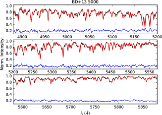
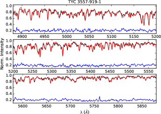
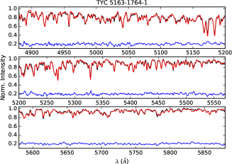
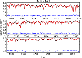
Figure 1: Observed (black) and best-matched synthetic spectrum (red) for each target stars. Residuals from the best-matched spectrum are shown in blue and shifted by 0.2 upwards for the sake of simplicity.

Inspecting Table 1, one can notice non-stable radial velocities for each target. Difference between measured maximum and minimum radial velocities is the smallest and about 17 km s^-1 for BD+11 3024, but much larger for the others. This could be result of a motion on a Kepler orbit, i.e. each star may actually be a member of an SB1 system. Although the clear difference between measured radial velocities of each individual star, we can not check this possibility with a preliminary orbital solution due to the less number of observed spectra sparsely distributed in time. However, we plot phase-folded radial velocities of each target in the appendix, for visual evaluation of radial velocity patterns with respect to the calculated photometric periods (see Section 3.3.2 and Table 5).

2.3 Spectral types and features

We compare spectra of target stars with the observed template spectra of 35 Peg and $\theta$ Psc to determine spectral type of each target. We choose a single observed spectrum for each target, which has the highest S/N, for comparison. In the first step we observe that the spectrum of 35 Peg provides close match to the spectra of TYC 3557-919-1, TYC 5163-1764-1 and BD+11 3024, thus indicating K0 III spectral type, while spectrum of $\theta$ Psc is similar to the spectra of BD+13 5000 and pointing out K1 III spectral type. In the second step, we adopt previously determined atmospheric parameters of 35 Peg and $\theta$ Psc (Sharma et al. 2016), as initial atmospheric parameters of corresponding target star, and switch to the spectrum synthesizing method to find the best matching synthetic spectrum to the observed spectrum of each target. Atmospheric parameters of the best matching synthetic spectrum is adopted as the final atmospheric parameters of the corresponding target.

We use the latest version of python framework $iSpec$ (Blanco-Cuaresma et al. 2014), which includes different spectrum synthesis codes, model atmospheres and line lists. In our case, we adopt SPECTRUM code (Gray & Corbally 1994) in conjunction with MARCS model atmospheres (Gustafsson et al. 2008) and the updated line list from Vienna Atomic Line Database (VALD, Ryabchikova et al. 2015). We calculate synthetic spectra for effective temperatures between 4000–5500 K with a step of 250 K, log$g$ value between 2.0–4.5 with a step of 0.5, and metallicity values ([M/H]) between $-$1.0 and 0.0 in steps of 0.25. We convolve each synthesized spectrum with a proper Gaussian line-spread function to match the resolution of TFOSC spectra. Then, we re-normalize the observed spectrum with respect to the instrumentally broadened synthetic spectrum, in order to compensate continuum level uncertainty coming from normalization by cubic splines in IRAF. Finally, we compare synthesized spectrum with the re-normalized observed spectrum by considering residuals. Since numerical fitting methods are not very efficient due to the resolution of TFOSC spectra, we only calculate synthetic spectra for available MARCS models, and refrain from any interpolation between the available model atmospheres. In the whole process, we keep micro-turbulence velocity fixed at 2 km s^-1. Considering resolution and S/N of TFOSC spectra, and grid steps of MARCS models for effective temperature, log$g$ and metallicity, we estimated uncertainties as 200 K in $T_{\rm eff}$, 0.5 in log$g$ and 0.25 in $[$M/H$]$. We list the atmospheric parameters of the synthetic spectra, that provides the closest match to the observed spectra of the target stars, in Table 2. In Figure 1, we plot observed and best-matched spectra at optical wavelengths, together with residuals from the best-matched synthetic spectra.

Table 2: Final atmospheric parameters of target stars. Sp denotes estimated spectral type.

Star	$T_{\rm eff}$	log$g$	$[$M/H$]$	Sp.
	(K)	(cgs)
BD+13 5000	4750	3.5	0.0	K0IV
TYC 3557-919-1	4750	3.0	0.0	K0III-IV
TYC 5163-1764-1	4500	2.5	-0.5	K2III
BD+11 3024	4750	3.0	-0.5	K0III-IV

We observe noticeable spectral characteristics of H_α and Ca ii H& K lines, which are sensitive to the chromospheric activity in cool stars. In Figure 2, we plot observed spectra around these lines. For all stars, Ca ii H& K lines are in form of emission. Very strong emission in Ca ii H& K lines, which exceeds continuum, and varying H_α profiles are remarkable for BD+13 5000 and TYC 3557-919-1, while BD+11 3024 and TYC 5163-1764-1 show variable H_α line profiles, but usually in form of filled absorption, which can be concluded by comparing their line profiles with the template star spectrum. Considering variable strength of emission features at different observation epochs, these features appear to be modulated with the rotation of the star. These spectral features and atmospheric parameters of the target stars clearly indicate chromospheric activity.

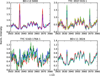
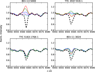
Figure 2: Observed spectra around Ca ii H& K lines (left four plots) and H_α line (right four plots). For each star, we plot all observed spectra with continuous lines in different colors, indicating different Julian dates given in Table 1. In H_α plots, note that we over plot observed spectrum of 35 Peg with thick dashed line for BD+13 5000, while the same thick dashed line denotes observed spectrum of $\theta$ Psc in the remaining plots.

3 Photometry

We collect differential $V$ photometry of our target stars with respect to a proper nearby comparison and check stars. We list basic data of all program stars in Table 3.

Table 3: Basic data of program stars. $V$ magnitudes and $B-V$ colours are from Tycho-2 catalogue (Høg et al. 2000), while $JHK$ magnitudes are from 2MASS All Sky Catalog of point sources (Cutri et al. 2003).

Star	Identifier	$\alpha$ (2000)	$\delta$ (2000)	$V$	$B-V$	$J$	$H$	$K$
Variable	BD+13 5000	22h 50m 24s	$+$14∘ 31′ 43′′	1061	113	8455	7895	7748
Comparison	2MASS 22502241+1434264	22h 50m 22s	$+$14∘ 34′ 26′′	—	—	11105	10946	10858
Check	BD+13 5001	22h 50m 30s	$+$14∘ 36′ 45′′	994	031	9276	9183	9124
Variable	TYC 3557-919-1	19h 43m 40s	$+$46∘ 40′ 03′′	1122	100	9232	8684	8536
Comparison	2MASS 19432561+4641206	19h 43m 26s	$+$46∘ 41′ 21′′	—	—	10135	9730	9617
Check	2MASS 19430979+4642507	19h 43m 10s	$+$46∘ 42′ 51′′	—	—	11947	11852	11827
Variable	TYC 5163-1764-1	20h 23m 34s	$-$01∘ 45′ 02′′	11335	133	—	—	—
Comparison	TYC 5163-1960-1	20h 23m 06s	$-$01∘ 35′ 08′′	1140	141	9625	9101	8984
Check	TYC 5163-1652-1	20h 23m 09s	$-$01∘ 42′ 16′′	1170	106	9924	9424	929
Variable	BD+11 3024	16h 41m 53s	$+$11∘ 40′ 21′′	1013	110	7890	7294	7077
Comparison	BD+11 3026p	16h 42m 26s	$+$11∘ 40′ 55′′	1059	056	9467	9188	9132
Check	BD+11 3026	16h 42m 28s	$+$11∘ 41′ 35′′	990	044	8953	8773	8698

Differential $V$ photometry comes from three sources. The first and the second sources are The All Sky Automated Survey (ASAS), and All-Sky Automated Survey for Supernovae Sky Patrol (ASAS-SN, Shappee et al. 2014; Kochanek et al. 2017) databases, and the third source is our Bessell $V$ CCD observations obtained at TNO.

3.1 ASAS and ASAS-SN photometry

We extract all available $V$-band photometric data of program stars from ASAS and ASAS-SN databases. Since we only have differential magnitudes from T60 observations, we convert standard magnitudes to differential magnitudes in order to evaluate observations on a common scale. We calculate average standard $V$ magnitude of each comparison star in the databases, and subtract it from each individual standard $V$ magnitudes of corresponding target star, thus obtain differential magnitudes in the sense of variable-minus-comparison. We estimate the precision of differential magnitudes with respect to the check-minus-comparison magnitudes. For check-minus-comparison measurements, we consider observing nights where simultaneous measurements from both check and comparison stars are available at exactly the same Julian date, and then obtain check-minus-comparison magnitudes. We list a brief information on collected data from ASAS and ASAS-SN databases in Table 4.

Table 4: Brief information on data collected from ASAS, ASAS-SN databases and T60 telescope. N and $\sigma$ show number of data points and standard deviation calculated from check-minus-comparison measurements for corresponding star.

	ASAS
Star	HJD range	N	$\sigma$
	(24 00000+)		(mag)
BD+13 5000	52765-55167	252	0.066
TYC 3557-919-1	—	—	—
TYC 5163-1764-1	51985-55145	369	0.045
BD+11 3024	52688-55093	357	0.033
	ASAS-SN
Star	HJD range	N	$\sigma$
	(24 00000+)		(mag)
BD+13 5000	56216-57932	354	0.029
TYC 3557-919-1	56695-57950	371	0.009
TYC 5163-1764-1	56389-57931	387	0.009
BD+11 3024	56337-57930	373	0.005
	T60
Star	HJD range	N	$\sigma$
	(24 00000+)		(mag)
BD+13 5000	56506-57365	164	0.010
TYC 3557-919-1	56536-57731	220	0.014
TYC 5163-1764-1	56533-57285	140	0.012
BD+11 3024	56532-57534	107	0.007

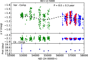
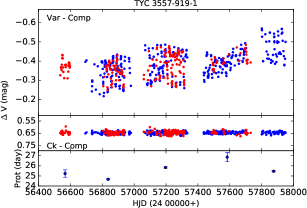
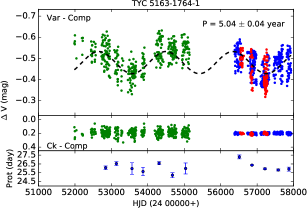
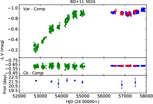
Figure 3: Differential photometry of program stars. Var, comp and ck denote variable, comparison and check stars, respectively. Black dashed lines inside plot windows of BD+13 5000 and TYC 5163-1764-1 indicate estimated period for long term brightness variation. The estimated periods are shown in each window together with their uncertainties. Green, red and blue filled points show photometry from ASAS, T60, and ASAS-SN, respectively. Lowermost panel of each window shows seasonal photometric periods (see Section 3.3.2, and Table 5).

3.2 T60 photometry

We collect Bessell $V$ CCD observations with 0.6 m robotic telescope (T60) at TNO, equipped with 2048 $\times$ 2048 pixels FLI ProLine 3041–UV CCD camera with a pixel size of 15 $\times$ 15 $\mu m^{2}$. We reduce automatically obtained CCD images with $ccdred$ package in IRAF environment, following bias subtraction and then flat field division of science frames. The CCD has an efficient cooling system, which cools down the CCD to $-$60 C and strictly stabilizes it during the whole night, hence bias and dark frame counts are almost same and we do not apply dark subtraction. We extract magnitudes of program stars from reduced science frames with $phot$ package in IRAF. Since comparison stars are just a few arc minutes away from target stars, we did not apply atmospheric extinction correction. In Table 4, we tabulate the brief information on our T60 observations.

We present T60, ASAS and ASAS-SN $V$ observations in Figure 3. Lower precision of ASAS measurements is noticeable compared to the T60 and ASAS-SN observations. Although the observational scatter can be as large as amplitude of individual light curves for ASAS data, it still confirms global stability of comparison stars, but with lower precision. T60 and ASAS-SN data provide further confirmation for the stability of comparison stars, with better precision.

3.3 Photometric analysis

3.3.1 Global photometric variation

We observe variable mean brightness and light curve amplitude for all targets. BD+13 5000 and TYC 5163-1764-1 exhibit cyclic mean brightness variation in time. Application of Lomb-Scargle periodogram (Lomb 1976; Scargle 1982) using $scipy$ package under $Python$ environment leads to 8.0$\pm$0.3 and 5.04$\pm$0.04 year cycle period for BD+13 5000 and TYC 5163-1764-1, respectively. No evidence is found for mean brightness variation with a longer period. In the case of TYC 3557-919-1, collected data cover only four years of time range, and variation pattern does not show any cyclic variation, but a $\sim$01 global brightening trend.

On the other hand, BD+11 3024 exhibits a striking increase in global brightness in ASAS photometry. The amount of increase is $\sim$07 and this increase is accompanied with a variable light curve amplitude from season to season. T60 and ASAS-SN observations show that the star somehow maintains its maximum brightness observed at the end of ASAS data. We apply second order polynomial fit to the ASAS data of the star, and linear fit to ASAS-SN and T60 data, to de-trend the whole light curve, and search for a signal of any cyclic brightness variation. Application of Lomb-Scargle periodogram to the de-trended data indicates $2.87\pm 0.12$ year cyclic variation with an amplitude of 003, which is shown in Figure 4.

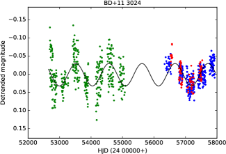
Figure 4: 2.87-yr cyclic brightness variation (black curve) detected in the de-trended photometric data of BD+11 3024. Meaning of colors are the same as Figure 3.

Table 5: Brightness levels and photometric periods found from application of the ANOVA method to the seasonal light curves. In the first four columns, set number, beginning, end and mean heliocentric Julian dates of the corresponding light curve are given. Photometric period and its uncertainty ($P$ and $\sigma~{}(P)$) are in unit of day. The maximum, minimum and mean brightnesses, and the light curve amplitude ($A$) are given in magnitudes. In the last column, $N$ shows number of data points used in the analysis.

BD+11 3024
Set	HJD min.	HJD max.	HJD mean	$P$	$\sigma~{}(P)$	max	min	mean	$A$	$N$
	(24 00000+)	(24 00000+)	(24 00000+)
1	52688.8799	52909.4910	52799.1855	21.79	0.11	-0.323	-0.206	-0.265	0.117	65
2	53415.8809	53634.4802	53525.1806	21.60	0.16	-0.650	-0.553	-0.602	0.097	62
3	53794.8888	53909.7268	53852.3078	21.14	0.97	-0.677	-0.622	-0.649	0.055	39
4	54154.8879	54363.4964	54259.1922	21.90	0.39	-0.825	-0.731	-0.778	0.094	57
5	54520.8874	54730.4803	54625.6839	21.84	0.05	-0.938	-0.831	-0.884	0.107	60
6	54881.8918	55092.4985	54987.1952	21.46	0.29	-0.952	-0.874	-0.913	0.078	38
7	56789.5162	56896.2329	56842.8746	20.88	0.86	-0.926	-0.875	-0.901	0.051	37
8	57434.6040	57533.3902	57483.9971	21.38	0.99	-0.964	-0.923	-0.943	0.041	27
BD+13 5000
Set	HJD min.	HJD max.	HJD mean	$P$	$\sigma~{}(P)$	max	min	mean	$A$	$N$
	(24 00000+)	(24 00000+)	(24 00000+)
1	52764.9261	52989.5301	52877.2281	18.51	0.61	-1.378	-1.320	-1.349	0.058	52
2	53512.9205	53717.5263	53615.2234	18.08	0.04	-1.507	-1.263	-1.385	0.244	45
3	54250.9308	54443.5358	54347.2333	18.34	0.02	-1.506	-1.062	-1.284	0.444	52
4	54601.9120	54811.5315	54706.7218	18.04	0.02	-1.360	-1.047	-1.203	0.313	50
5	54967.9262	55166.5666	55067.2464	18.09	0.03	-1.451	-1.063	-1.257	0.388	31
6	56397.1295	56669.1541	56533.1418	17.95	0.11	-1.352	-1.160	-1.256	0.192	110
7	56782.0933	57020.6935	56901.3934	18.26	0.03	-1.424	-1.171	-1.298	0.253	132
8	57132.1243	57378.7314	57255.4279	18.09	0.04	-1.349	-1.159	-1.254	0.190	161
9	57496.1318	57745.6977	57620.9148	18.20	0.02	-1.337	-1.094	-1.215	0.243	83
TYC 3557-919-1
Set	HJD min.	HJD max.	HJD mean	$P$	$\sigma~{}(P)$	max	min	mean	$A$	$N$
	(24 00000+)	(24 00000+)	(24 00000+)
1	56536.2497	56597.1793	56566.7145	25.24	0.36	-0.431	-0.292	-0.361	0.139	29
2	56694.1694	56979.6930	56836.9312	24.67	0.05	-0.412	-0.251	-0.332	0.161	179
3	57060.6618	57333.7025	57197.1822	25.84	0.06	-0.462	-0.283	-0.373	0.179	203
4	57437.1658	57731.1923	57584.1791	26.86	0.46	-0.432	-0.363	-0.398	0.069	132
5	57801.1689	57949.8032	57875.4860	25.46	0.06	-0.567	-0.398	-0.483	0.169	48
TYC 5163-1764-1
Set	HJD min.	HJD max.	HJD mean	$P$	$\sigma~{}(P)$	max	min	mean	$A$	$N$
	(24 00000+)	(24 00000+)	(24 00000+)
1	52721.8999	52964.5131	52843.2065	26.07	0.20	-0.594	-0.463	-0.528	0.131	66
2	53082.9093	53191.7672	53137.3383	26.54	0.22	-0.541	-0.392	-0.467	0.149	25
3	53454.9023	53677.5511	53566.2267	25.98	0.65	-0.457	-0.382	-0.420	0.075	61
4	53823.8992	53913.7795	53868.8394	25.64	0.48	-0.535	-0.407	-0.471	0.128	22
5	54191.8947	54428.5135	54310.2041	26.59	0.18	-0.604	-0.488	-0.546	0.116	53
6	54559.9012	54792.5118	54676.2065	25.23	0.29	-0.574	-0.494	-0.534	0.080	63
7	54931.8943	55145.5269	55038.7106	25.99	0.62	-0.593	-0.500	-0.546	0.093	42
8	56389.0940	56636.1713	56512.6327	27.29	0.22	-0.553	-0.461	-0.507	0.092	102
9	56735.1287	56984.6854	56859.9071	26.36	0.07	-0.526	-0.376	-0.451	0.150	118
10	57094.9021	57337.5197	57216.2109	25.95	0.09	-0.501	-0.364	-0.433	0.137	170
11	57457.1418	57705.5100	57581.3259	25.82	0.11	-0.525	-0.406	-0.465	0.119	91
12	57817.1547	57930.9784	57874.0666	25.92	0.23	-0.554	-0.400	-0.477	0.154	46

3.3.2 Photometric period and seasonal brightness variations

For each target, we determine minimum, maximum and mean brightnesses of seasonal light curves, as well as corresponding light curve amplitudes and photometric periods. In most cases, light curves are asymmetric, which is a common feature observed in light curves of chromospherically active stars. Hence, application of periodogram methods based on Fourier transform would result in multiple periods, i.e. main period, which corresponds to the photometric period, and its harmonics. However, application of statistical methods, such as Phase Dispersion Minimization (PDM, Stellingwerf 1978) and Analysis of Variances (ANOVA, Schwarzenberg-Czerny 1996), are more efficient to find a single period which would be the single representative period for the observed variation, without any additional periods (i.e. harmonics). In the scope of our study, we adopt ANOVA method. In the first step of the analysis, we determine photometric period of each observing season. Second, we phased the light curve of that season with its resulting photometric period. Finally, we fit a cubic spline to the phase-folded light curve, and determine minimum and maximum brightnesses. The mean brightness and the amplitude of the light curve are calculated from determined minimum and maximum brightnesses. We tabulate our analysis results in Table 5. We plot seasonal light curves of each target in the appendix.

For any of the target star, the number of sets listed in Table 5 is insufficient for evaluation of any correlation between parameters, e.g. the photometric period and the light curve amplitude, the amplitude and the brightness, or the photometric period and the mean brightness. For example, plotted photometric periods in Figure 3 do not seem to be correlated with the mean brightness. However, considerable discontinuities in the photometric data, and observing seasons where the photometric period could not be determined due to the very low light curve amplitude reduce the number of useful datasets for analysis, thus may cause misinterpretation of the real situation. Still, we find average photometric periods as 2149, 1817, 2561 and 2611 for BD+11 3024, BD+13 5000, TYC 3557-919-1 and TYC 5163-1764-1, respectively. We use the distribution range of photometric periods and estimate $\Delta P/P=(P_{max}-P_{min})/P_{eq}$, where $P_{max}$ and $P_{min}$ denote calculated maximum and minimum photometric periods for corresponding target, and $P_{eq}$ is equatorial rotation period, which is adopted as the mean value of the measured rotation periods for each target, given in Table 5. Using periods listed in Table 5, we find $\Delta P/P$ values as 0.047, 0.031, 0.086, 0.079 for BD+11 3024, BD+13 5000, TYC 3557-919-1 and TYC 5163-1764-1, respectively.

4 Summary and discussion

We present analysis of spectroscopic and long-term photometric observations of four cool stars, BD+11 3024, BD+13 5000, TYC 3557-919-1 and TYC 5163-1764-1. Strong emission in H_α and Ca ii H& K lines, which exceeds the continuum in the case of BD+13 5000 and TYC 3557-919-1, and remarkable changes in mean brightness and light curve amplitude clearly indicate chromospheric activity on these stars. Observed emissions appear to be rotationally modulated. Furthermore, non-stable radial velocities of the target stars indicate that they might possibly be a member of a binary system. However, binary nature of these stars and rotational modulation of the emission features need to be confirmed by further observations, which would cover at least a rotational cycle.

Analysis of seasonal light curves makes possible to trace seasonal photometric periods. Distribution range of photometric periods enables us to calculate $\Delta P/P$, which gives some hints on the lower limit of the differential rotation, and spot evolution in time, which could also alter the distribution of the photometric period in time. Growth and decay of spot regions at different latitudes and longitudes (i.e. temporal and spatial evolution of spots) may cause variation in photometric period (see, e.g. Fekel et al. 2002). Less number of datasets in Table 5 do not allow one to arrive at any conclusive results, however, we notice that calculated $\Delta P/P$ values are larger than the values of spotted stars studied in Hall & Busby (1990).

We find average rotational period of BD+11 3024 as 2149. Considering the uncertainties of seasonal periods in the Table 5, it is in agreement with the period reported by Bernhard (2008). We observe more precise agreement in the case of BD+13 5000, where our average period is 1817 and the period reported by Kiraga (2012) is 1814. The average photometric period of TYC 3557-919-1 found in this study is 2561, while it was found as 2508 by Bernhard (2008). In summary, we observe no discrepancies between average photometric periods found in this study and the literature values.

Below, we discus our further findings for each star, in a separate paragraph.

BD+13 5000. Our atmospheric analysis indicates K0IV spectral type for the star. Measured radial velocities are distributed in a range of 90 km s^-1, indicating that the star could be a spectroscopic binary. Very strong emission, which exceeds the continuum, is observed in H_α and Ca ii H& K lines. These features are accompanied with a cyclic variation in the mean brightness with a period of $8.0\pm 0.3$ year, which repeats itself for two times in the time base of the current photometric data, and indicates an activity cycle. In most cases, light curve amplitudes are larger than 019. All these findings suggest a very strong and cyclic chromospheric activity.

TYC 3557-919-1. Analysis of TFOSC spectra indicates K0III-IV spectral type. Radial velocities appear to be variable, where the maximum difference among the measurements is to be 52 km s^-1, suggesting the possibility of being spectroscopic binary. Similar to BD+13 5000, H_α and Ca ii H& K lines exhibit very strong emission that exceeds the continuum. Available photometric data cover four years and only indicate a global brightening trend of $\sim$01, with a seasonal light curve amplitude usually between 01 and 02. These are clear evidence of very strong chromospheric activity.

TYC 5163-1764-1. Spectral type of the star is found as K2III. As in the cases of BD+13 5000 and TYC 3557-919-1, we observe unstable radial velocities in a range of 49 km s^-1, indicating possibility of being spectroscopic binary. Emission observed in H_α and Ca ii H& K lines are weaker compared to BD+13 5000 and TYC 3557-919-1, but still clearly observed, reaching to the continuum level around Ca ii K line. We find cyclic mean brightness variation with a period of $5.04\pm 0.04$ year, repeating itself more than three times in the time span of the photometric data. Observed light curve amplitudes are between 0075 and 0154. These findings suggest strong and cyclic chromospheric activity.

BD+11 3024. TFOSC spectra of this star indicate K0III-IV spectral type. Measured radial velocities are distributed between smaller range (17 km s^-1) compared to the other target stars, weakly indicates possibility of being spectroscopic binary. Strengths of H_α and Ca ii H& K emissions of the star are very similar to the observed emissions in TYC 5163-1764-1. Photometric data of the star exhibit very dramatic brightness increase ($\sim$07) accompanied with a $2.87\pm 0.12$ year cyclic brightness variation with 003 amplitude. The star might have multiple cycles if the global brightness increase is part of a longer term cyclic brightness change with a larger amplitude. This would not be surprising since multiple cycles appear to be observed often in active stars (Oláh et al. 2009). Seasonal light curve amplitude, usually below 01, and interesting brightness variations make this star an attractive target for further studies.

Spectroscopic and photometric characteristics of BD+13 5000, TYC 3557-919-1 and TYC 5163-1764-1 are similar to the typical RS CVn stars with strong emission in their Ca ii H& K lines, cyclic mean brightness variation and remarkable light curve amplitude, e.g. V1149 Ori (Fekel & Henry 2005; Jetsu et al. 2017), HD 208472 (Özdarcan et al. 2010, 2016), FG UMa (Fekel et al. 2002; Özdarcan et al. 2012), and many other targets studied in Oláh et al. (2009) and Jetsu et al. (2017). Individually, photometric behaviour of BD+11 3024 resembles RS CVn binary IS Vir (Fekel et al. 2002; Oláh et al. 2013), which possesses similar light curve amplitude, and a long term variation with an estimated period of 5-6 years (Oláh et al. 2013). Dramatic changes in the mean brightness of BD+11 3024 suggests strong spot activity. In this case, low light curve amplitude could be explained by either assuming that the distribution of spots is usually homogeneous on the surface of the star, or assuming the inclination of the rotational axis is low, as in the case of IS Vir, thus causing low light curve amplitude.

High resolution optical spectroscopy is required to determine more precise atmospheric properties and projected rotational velocities, as well as to trace radial velocities in order to check whether each of these stars is single or a member of a binary system. Determination of projected rotational velocities from high resolution spectroscopy would help to restrict the stellar radius, which is one of the key parameter to calculate stellar luminosity, i.e. vertical position of a star in HR diagram. Further time series photometric observations would enable one to trace activity cycles and study the relation between cycle length and rotation period (e.g. Oláh & Strassmeier 2002), as well as surface differential rotation via distribution of seasonal photometric periods in time (Hall & Busby 1990; Özdarcan et al. 2010, 2012).

Appendix A Seasonal light curves and phase folded radial velocities

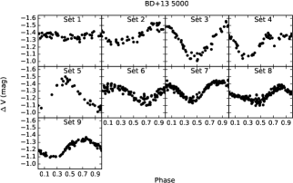
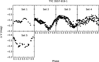
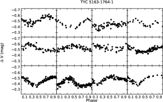
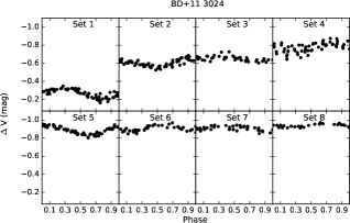
Figure 5: Phase folded seasonal light curves of the target stars. Phase folding is done with the calculated photometric period listed in Table 5 and heliocentric Julian date of the initial data point of corresponding light curve.

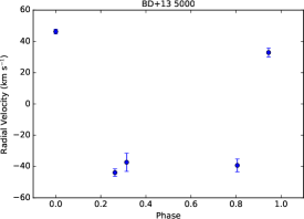
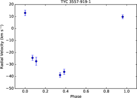
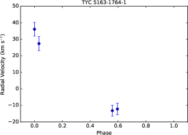
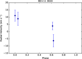
Figure 6: Phase folded radial velocities of the target stars. Phase folding is done with respect to the time of the observed positive maximum velocity (ephemeris, see Table 1) and calculated mean photometric period read from Table 5.