Phononic Rogue Waves

Abstract

We present a theoretical study of extreme events occurring in phononic lattices. In particular, we focus on the formation of rogue or freak waves, which are characterized by their localization in both spatial and temporal domains. We consider two examples. The first one is the prototypical nonlinear mass-spring system in the form of a homogeneous Fermi-Pasta-Ulam-Tsingou (FPUT) lattice with a polynomial potential. By deriving an approximation based on the nonlinear Schrödinger (NLS) equation, we are able to initialize the FPUT model using a suitably transformed Peregrine soliton solution of the NLS, obtaining dynamics that resembles a rogue wave on the FPUT lattice. We also show that Gaussian initial data can lead to dynamics featuring rogue wave for sufficiently wide Gaussians. The second example is a diatomic granular crystal exhibiting rogue wave like dynamics, which we also obtain through an NLS reduction and numerical simulations. The granular crystal (a chain of particles that interact elastically) is a widely studied system that lends itself to experimental studies. This study serves to illustrate the potential of such dynamical lattices towards the experimental observation of acoustic rogue waves.

I Introduction

Extreme wave events, such as freak or rogue waves, are waves that seem to appear out of nowhere, and then vanish without a trace r1 ; r2 ; r3 . The term rogue wave was first coined to describe an ocean wave that has an amplitude greater than twice the significant wave height r1 . Based on the classical description of waves that assumes a Rayleigh distribution of wave heights, a rogue wave should be an extremely rare event r1 . The measurement of an ocean rogue wave (the Draupner wave) in 1995 initiated an intense interest in the subject of extreme events. It has been found that ocean rogue waves occur more regularly than the statistical description predicts r1 , and a number of alternative mechanisms for the formation of rogue waves has been produced r1 . One such approach is through the derivation of simple modulation equations such as the nonlinear Schrödinger (NLS) equation from the underlying equations of motion NLS . The Peregrine soliton solution of the focusing NLS equation sits atop a finite background, and is localized in both space and time Peregrine . The maximum amplitude of the Peregrine soliton is three times greater than the background upon which it sits, and is therefore a prominent rogue wave candidate. Such structures have been studied in various media, including nonlinear optics o1 ; o2 ; o3 ; o4 , mode-locked lasers laser , superfluid helium super , hydrodynamics hydro1 ; hydro2 ; hydro3 , Faraday surface ripples Faraday , parametrically-driven capillary waves cap , plasmas plasmas , ultra-cold gases stathis and electrical transmission lines lefthand . A unifying theme of these varied physical settings of rogue waves is the relevance of the NLS setting as an approximate model equation. Rogue waves in discrete systems are far less studied. One example of such a study concerns rogue waves in the integrable Ablowitz-Ladik lattice RogueAL , which is known to have an exact solution that has similar properties as the NLS Peregrine soliton. At the level of granular systems, the pioneering work of sen2 was the first one to recognize the potential of such systems for unusually large (rogue) fluctuations in late time dynamics, in the absence of dissipation.

The present study concerns a different discrete system, namely phononic lattices, which are systems that manipulate pressure waves (as opposed to photonic latices in which light waves are manipulated). Arguably, one of the most prototypical phononic lattice is the Fermi-Pasta-Ulam-Tsingou (FPUT) lattice, which describes a one-dimensional system of masses coupled through weakly nonlinear springs FPU55 . While the amount of research efforts in the direction of the FPUT lattice is immense (see the book FPUbook , but also the recent review PGlattice ), rogue waves in FPUT lattices have not been reported on, to the best of our knowledge. In the small amplitude limit, the NLS equation is once again a valid modulation equation, suggesting that Peregrine-soliton-type dynamics are possible in phononic lattices.

To demonstrate that a phononic rogue wave could in principle be observed experimentally, we conduct a study in the case of an one-dimensional chain of beads interacting through Hertzian contacts, i.e. granular crystals. Over the last two decades, granular crystals have received considerable attention, as is now summarized in a wide range of reviews nesterenko1 ; sen08 ; theocharis_review ; vakakis_review ; gc_review ; yuli_book ; ptpaper . Granular crystals are remarkably tunable, which permits one to access weakly or strongly nonlinear dynamic responses. At the same time, it is possible to easily access and arrange the media in a wide range of configurations (homogeneous, periodic, chains with impurities, chains with local resonators, disordered chains, and many others). These aspects make the study of granular crystals fascinating from both fundamental and applied perspectives ptpaper .

The remainder of the paper is structured as follows. In Sec. II, we examine a homogeneous FPUT lattice. We derive a focusing NLS equation, which describes the modulation of small amplitude and rapidly oscillating plane waves in time and space. The Peregrine soliton of the NLS equation is used to initialize the FPUT system which leads to rogue-like wave dynamics. The prediction based on the NLS approximation coincides with the numerical simulations of the FPUT lattice up until the formation of the large amplitude wave. While the NLS approximation sees a decreasing and “vanishing” of the large amplitude wave back towards the background, the presence of a modulational instability causes the formation of outward propagating waves from the center of the lattice. We also explore generalized pulse like initial data (in the form of Gaussian wave packets), which can lead to wide variety of behavior including soliton dynamics, breathing dynamics, and rogue wave dynamics. The amplitude of the initial conditions “selects” the type of observed dynamics. In Sec. III we consider a diatomic granular crystal lattice. Using a focusing NLS equation derived as an envelope approximation of this diatomic chain, we once again use the Peregrine soliton solution of the NLS equation to initialize the lattice dynamics. We find qualitatively similar behavior to that reported for the homogeneous FPUT lattice for all mass ratios tested. A noteworthy finding is that the sensitivity to boundary effects appears to depend on the chosen mass ratio. Sec. IV draws conclusions and discusses future directions.

II Homogeneous Fermi-Pasta-Ulam-Tsingou Lattices

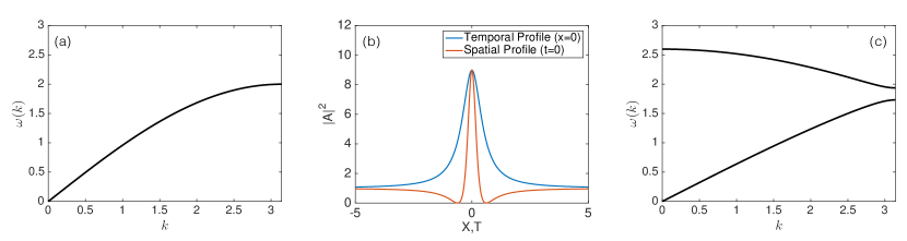
Figure 1: (a) Dispersion relation for the monomer FPUT lattice with $K_{2}=1$, which consists of an acoustic branch only. (b) The spatial profile of the Peregrine soliton at $t=0$ and the temporal profile at $x=0$. (c) Dispersion relation for the dimer FPUT lattice with $K_{2}=3/2$ and $\rho=0.8$, which consists of an acoustic branch (lower branch) and optical branch (upper branch).

II.1 Theoretical Set-up

The prototypical Fermi-Pasta-Ulam-Tsingou (FPUT) lattice has the form

$$\ddot{u}_{n}=V^{\prime}(u_{n+1}-u_{n})-V^{\prime}(u_{n}-u_{n-1})$$ (1)

with

$$V^{\prime}(x)=K_{2}x+K_{3}x^{2}+K_{4}x^{3},$$ (2)

where $n\in I$, with $I$ a countable index set, and $u_{n}=u_{n}(t)\in{\mathbb{R}}$ is the displacement of the $n$th particle from equilibrium position at time $t$. Equation (1) with $I={\mathbb{Z}}$ has the Hamiltonian

$$H=\sum_{n\in{\mathbb{Z}}}\frac{1}{2}\dot{u}_{n}^{2}+V(u_{n+1}-u_{n}).$$

The linear problem (i.e. when $K_{3}=K_{4}=0$) is solved by

$$u_{n}(t)=e^{i(kn+\omega t)}$$

for all $k\in[0,\pi]$, where $\omega$ and $k$ are related through the dispersion relation,

$$\omega(k)^{2}=4K_{2}\sin^{2}(k/2),$$

such that the cutoff point of the acoustic band is $2\sqrt{K_{2}}$, see Fig. 1(a). Motivated by prior works on rogue waves where the Peregrine soliton is used to describe the formation of such structures, we first derive the NLS equation from Eq. (1). When deriving the NLS equation as a modulation equation, one uses the multiple scale ansatz

$$u_{n}(t)\approx\psi_{n}(t):=\varepsilon\left(B(X,T)+\left[A(X,T)E+c.c.\right]\right)\,,\qquad E=e^{i(k_{0}n+\omega_{0}t)},\quad X=\varepsilon(n+ct),\quad T=\varepsilon^{2}t,$$ (3)

where $\varepsilon\ll 1$ is a small parameter, effectively parametrizing the solution amplitude (and also its inverse width). Directly substituting this ansatz into Eq. (1) and equating the various orders of $\varepsilon$ leads to the dispersion relation $\omega_{0}=\omega(k_{0})$, at $\mathcal{O}(\varepsilon)$ the group velocity relation $c=\omega^{\prime}(k_{0})$, at $\mathcal{O}(\varepsilon^{2})$ and the nonlinear Schrödinger equation

$$i\partial_{T}A(X,T)+\nu_{2}\partial_{X}^{2}A(X,T)+\nu_{3}A(X,T)|A(X,T)|^{2}=0,$$ (4)

at $\mathcal{O}(\varepsilon^{3})$, where $\nu_{2}=-\omega^{\prime\prime}(k_{0})/2>0$ and $\nu_{3}$ is a lengthy wavenumber-dependent expression. Full details of the derivation of the NLS equation starting from Eq. (1), including the higher-order terms of the ansatz, can be found e.g. in Schn10 ; Huang1 ; Huang2 . Since we seek standing wave solutions, we choose the wavenumber to be at the edge of the acoustic band $k_{0}=\pi$, such that the group velocity vanishes, $\omega_{0}=2\sqrt{K_{2}}$, and

$$\left.\nu_{3}\right|_{k_{0}=\pi}=\frac{4}{K_{2}\sqrt{K_{2}}}(3K_{2}K_{4}-4K_{3}^{2})=b.$$

Since $\nu_{2}>0$, the NLS equation (4) will be focusing if $b>0$. For our numerical computations, we consider the case example of $K_{2}=K_{4}=1$ and $K_{3}=1/\sqrt{2}$ such that $\nu_{2}=1/4$ and $b=4$. The equation for $B(X,T)$ is defined in terms of $A(X,T)$,

$$\partial_{X}B(X,T)=\frac{4K_{3}(1-\cos(k))}{(\omega^{\prime}(k))^{2}-(\omega^{\prime}(0))^{2}}|A(X,T)|^{2}.$$ (5)

II.2 Peregrine Initial Data

The focusing NLS equation has the one-parameter family of Peregrine soliton solutions Peregrine given by

$$A(X,T)=\sqrt{\frac{P_{0}}{\nu_{3}}}\left(1-\frac{4(1+2P_{0}\,iT)}{1+\frac{2}{\nu_{2}}P_{0}X^{2}+4P_{0}^{2}T^{2}}\right)e^{iP_{0}T},$$ (6)

where $P_{0}>0$ is an arbitrary parameter. This solution is localized in space and time and has a maximum (located at $(x,t)=(0,0)$) that is three times greater than its background, which are the features we desire to describe a rogue wave, see Fig. 1(b). Using the Peregrine soliton for the envelope function and a wave number $k_{0}=\pi$, $K_{2}=K_{4}=1$ and $K_{3}=1/\sqrt{2}$ we arrive at the following approximation

$$u_{n}(t) = \frac{\sqrt{\eta}}{2}\left(1-\frac{4(1+2i\eta\,t)}{1+8\eta n^{2}+4(\eta t)^{2}}\right)e^{i(\pi n+(2+\eta)t)}+c.c.+\varepsilon B(\varepsilon n,\varepsilon^{2}t)\,,\qquad\eta=P_{0}\varepsilon^{2},$$ (7)

where $B$ is defined in Eq. (5). It will be convenient to represent the solution in the strain variable formulation, that is, $y_{n}=u_{n+1}-u_{n}$ since the term $B$ in the ansatz, which introduces a linear slope, will vanish. The parameter $\eta=P_{0}\varepsilon^{2}>0$ selects the background amplitude (since $|y_{n}(0)|\rightarrow 2\sqrt{\eta}$ as $n\rightarrow\pm\infty$) and the frequency of oscillation $2+\eta$, which lies above the cutoff of the acoustic band $\omega_{0}=2$.

To test the validity of the multiscale analysis, we perform numerical simulations of the FPUT model Eq. (1) using Eq. (7) as initial data. For instance, see Fig. 2 for a simulation with $\varepsilon=0.02$, $X\in[-40,40]$ and $T\in[-5,5]$. In this simulation, our initial time is $t=-5\varepsilon^{2}$, such that $t=0$ should correspond to a peak at the middle node $n=0$. The simulations are sensitive to the boundary conditions since the background is non-zero (we employ boundary conditions that are periodic in the strain). Therefore, we take a larger spatial domain to reduce the influence of the boundary, since we are mainly concerned with the core of the solution. For times before the rogue wave appears (i.e. $t<0$) the FPUT dynamics is predicted by the NLS dynamics (compare Fig. 2(a) and  2(b)). After the formation of the rogue wave, i.e., for $t>0$, the FPUT dynamics departs from the NLS prediction. In the FPUT case, the large amplitude portion of the wave breaks into smaller, but still large relative to the background, waves. We believe that the emergence of these waves stemming from the Peregrine soliton core is a byproduct of the modulational instability of the NLS background as transcribed into the FPUT lattice and as seeded by the large amplitude perturbation induced by the wave structure.

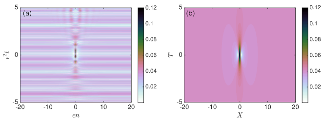
Figure 2: (a) Simulation of Eq. (1) with $\varepsilon=0.02$, $X\in[-40,40]$ and $T\in[-5,5]$ that is initialized with Eq. (3) with $A$ given by Eq. (6) with $P_{0}=1$. Color intensity corresponds to the strain $|y_{n}(t)|$. Notice that the space-time evolution here and in the figures that follow is given in terms of the rescaled variables $\varepsilon n$ and $\varepsilon^{2}t$ for space and time, respectively. (b) Corresponding NLS prediction $2\varepsilon|A(X,T)|$. Note that the background amplitude of $|y_{n}(t_{0})|$ is the same as $2\varepsilon|A(X,T_{0})|$.

II.3 Gaussian Initial Data

It has been shown through the rigorous work of bertola that Peregrine-like structures are a generic by-product of the so-called gradient catastrophe phenomenon that the (focusing) NLS is subject to for localized initial data in the semi-classical limit. This feature has led also to very clean recent observations of Peregrine solitons in optical systems suret . Also, at a numerical level, systematic explorations of Gaussian initial data have led to rogue-like waves in the focusing NLS equation for sufficiently broad Gaussians stathis . When sufficiently broad (so as to be rescalable to the semi-classical regime), the waves evolving through the equations of motion focus their energy to the center in a Peregrine structure. Even more remarkably, such initial data subsequently lead to the formation of an array of essentially identical (up to small corrections) Peregrine-like structures, arising at the poles of the so-called tritronquée solution of the Painévé I equation. On the other hand, if the Gaussian is sufficiently narrow, then a solution more akin to a soliton forms; see the top panel of Fig. 3 for a few examples. Here, we investigate if a similar phenomenology is possible in the FPUT lattice. More specifically, we consider initial data for the envelope function $A(X,T)$ of the form

$$A(X,T=0):=A_{G}(X)=\exp\left(\frac{-X^{2}}{4\sigma^{2}}\right).$$ (8)

In Fig. 3 results for simulations for the parameter values $\sigma\in\{20.1,10.5,2.5,1.3\}$ for $\varepsilon=0.1$ and $\varepsilon=0.05$ are shown. Note the strong resemblance to the NLS prediction, however, after the main peak forms, there is noticeable distortion between the NLS prediction and the actual FPUT dynamics, just as the case in the Peregrine example in the previous subsection. In this simulation the tails are decaying to zero, and thus any potential boundary effects should be minimal. These findings confirm once again the genericity of the gradient catastrophe scenario of bertola , although presumably the non-integrability of the present lattice distorts the “Christmas-tree” pattern of the subsequent Peregrines in comparison to the NLS paradigm. Nevertheless, the pattern is still clearly discernible and progressively reverts to breathing and ultimately to solitonic solutions as $\sigma$ decreases (i.e., along the horizontal direction). On the other hand, the trend of decreasing $\varepsilon$ (along the vertical direction) makes the patterns appear more and more “NLS-like” as is expected by the increased accuracy of the NLS approximation in the limit of small $\varepsilon$.

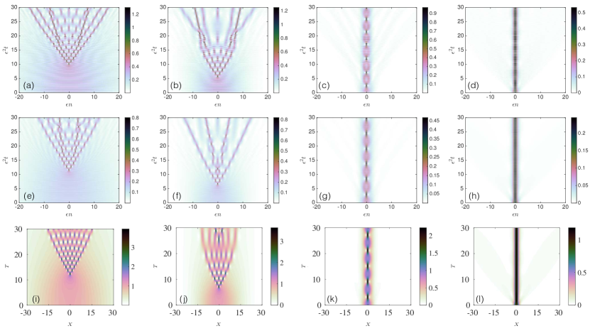
Figure 3: Simulation of Eq. (1) that is initialized with Eq. (3) with $A$ given by Eq. (8) with the following width parameters $\sigma=20.1$ for panels (a,e,i), $\sigma=10.5$ for panels (b,f,j), $\sigma=2.5$ for panels (c,g,k) and $\sigma=1.3$ for panels (d,h,l). In panels (a)-(d) the perturbation parameter value is $\varepsilon=0.1$. In panels (e)-(h) the perturbation parameter value is $\varepsilon=0.05$. Panels (i)-(l) correspond to the respective numerical simulations of the NLS equation with Gaussian initial data, see e.g. Ref. stathis .

III Diatomic Granular Crystal

III.1 Theoretical Set-up

We now turn our attention to another variant of the FPUT model that considers a so-called Hertzian contact nesterenko1 ; sen08 for the nonlinearity rather than the polynomial nonlinearity considered in Eq. (1). Such a nonlinearity is relevant in the description of granular crystals when only considering forces due to elastic compression between the particles. In this case, the model equations are

$$\ddot{u}_{n}=\frac{A_{n}}{m_{n}}[\delta_{0,n}+u_{n-1}-u_{n}]_{+}^{p}-\frac{A_{n+1}}{m_{n}}[\delta_{0,n+1}+u_{n}-u_{n+1}]_{+}^{p}\,,$$ (9)

where $u_{n}$ is the displacement of the $n$th particle measured from its equilibrium position in an initially compressed chain, $m_{n}$ is the mass of the $n$th particle, and $\delta_{n}=({F_{0}}/{A_{n}})^{1/p}$ is a static displacement for each particle that arises from the static load $F_{0}=\text{const}$. For spherical particles, the exponent is $p=3/2$ and the parameter $A_{n}$, which reflects the material and the geometry of the chain’s particles, has the form

$$A_{n}=\frac{4E_{n}E_{n+1}\sqrt{\frac{R_{n}R_{n+1}}{\left(R_{n}+R_{n+1}\right)}}}{3E_{n+1}\left(1-\nu_{n}^{2}\right)+3E_{n}\left(1-\nu_{n+1}^{2}\right)},$$ (10)

where $E_{n}$ is the elastic (Young) modulus of the $n$th particle, $\nu_{n}$ is its Poisson ratio, and $R_{n}$ is its radius. Important special cases of Eq. (9) include monoatomic (i.e., “monomer”) chains (in which all particles are identical, so $A_{n}=A$, $m_{n}=m$, and $\delta_{0,n}=\delta_{0}$), period-2 diatomic chains, and chains with impurities (e.g., a “host” monomer chain with a small number of “defect” particles of a different type). In a monomer chain with strong precompression, Eq. (9) is well approximated by the FPUT model Eq. (1). To see this, let $V^{\prime}(x)=-F(-x)$, and Taylor expand the nonlinearity $F(x)=[\delta_{0}+x]^{3/2}_{+}$ about $x=0$. This leads to

$$V^{\prime}(x)=-\delta_{0}^{3/2}+K_{2}x+K_{3}x^{2}+K_{4}x^{3},\qquad K_{2}=\frac{3}{2}\delta_{0}^{1/2},\quad K_{3}=-\frac{3}{8}\delta_{0}^{-1/2},\quad K_{4}=-\frac{3}{48}\delta_{0}^{-3/2}.$$ (11)

Thus, in the small amplitude limit (where the above Taylor expansion is valid), one can apply the same multiple scale analysis as in Sec. II. However, in the case of the coefficients given in (11) the linear and nonlinear coefficients of the NLS equation are respectively $\nu_{2}=-\omega^{\prime\prime}(\pi)/2>0$ and $\nu_{3}=(K_{2}K_{4}-4K_{3}^{2})/(K_{2}\sqrt{K_{2}})<0$, and thus, the relevant NLS equation for the monomer granular crystal is the defocusing NLS. While this case is interesting in its own right (allowing the existence of NLS dark solitons, and hence dark breathers of the granular crystal dark ; dark2 ), there are no Peregrine solitons. To obtain a focusing NLS equation (and hence the possibility of Peregrine solitons) we modify our lattice model such that there are additional branches in the dispersion. In particular, we seek a dispersion relation such that one branch has the opposite concavity of the acoustic branch of the monomer chain at $k=\pi$, namely that $-\omega^{\prime\prime}(\pi)/2<0$. Such is the case for the dimer granular crystal (see Fig. 1(c)) which consists of alternating particles of two types, so $A_{n}=A$, $\delta_{0,n}=\delta_{0}$, and the mass is $m_{n}=m$ for even $n$ and $m_{n}=M$ for odd $n$. In such a chain, the mass ratio $\rho=m/M$ is the only additional parameter beyond the monomer case. If we introduce new variables $v_{n}$ to represent the displacement of the even particles (e.g. $v_{n}=u_{2k}$) and $w_{n}$ to represent the displacement of the odd particles (e.g. $w_{n}=u_{2k+1}$), then we can re-write Eq. (9) as

$$\rho\ddot{v}_{n} = [1+w_{n-1}-v_{n}]_{+}^{3/2}-[1+v_{n}-w_{n}]_{+}^{3/2},$$ (12)

$$\ddot{w}_{n} = [1+v_{n}-w_{n}]_{+}^{3/2}-[1+w_{n}-v_{n+1}]_{+}^{3/2},$$ (13)

where we have re-scaled time and amplitude. We assume that $M>m$, such that the mass ratio $\rho<1$. Note that these equations under the assumption of small strain,

$$|w_{n-1}-v_{n}|\ll 1,\qquad|w_{n}-v_{n}|\ll 1$$

reduce to the dimer FPUT lattice,

$$\rho\ddot{v}_{n} = V^{\prime}(w_{n}-v_{n})-V^{\prime}(v_{n}-w_{n-1}),$$ (14)

$$\ddot{w}_{n} = V^{\prime}(v_{n+1}-w_{n})-V^{\prime}(w_{n}-v_{n}),$$ (15)

where

$$V^{\prime}(x)=K_{2}x+K_{3}x^{2}+K_{4}x^{3},\qquad K_{2}=\frac{3}{2},\quad K_{3}=-\frac{3}{8},\quad K_{4}=-\frac{3}{48}.$$

The linearized Eqs. (14) and (15) (i.e. where $K_{3}=K_{4}=0$) have solutions of the form $(v_{n},w_{n})^{T}=(v^{0},w^{0})^{T}e^{i(kn+\omega t)}$, where $k$ and $\omega$ are related through the dispersion relation

$$\omega(k)_{\pm}^{2}=K_{2}\left(1+\frac{1}{\rho}\right)\pm\sqrt{\left(1+\frac{1}{\rho}\right)^{2}-\frac{4}{\rho}\sin^{2}\left(\frac{k}{2}\right)},$$ (16)

where the minus and plus signs correspond to the acoustic and optical bands, respectively, of the dispersion relation, see Fig. 1(c). At the wavenumber $k=\pi$ the upper cutoff frequency of the acoustic band is $\omega_{-}(\pi)=\sqrt{2K_{2}}$ and the lower cutoff frequency of the optical band is $\omega_{+}(\pi)=\sqrt{2K_{2}/\rho}$. Since $\rho<1$ there is a band gap of size $\omega_{+}(\pi)-\omega_{-}(\pi)=\sqrt{\frac{2K_{2}}{\rho}}(1-\sqrt{\rho})$. In order to find a rogue wave, we proceed in the same way as in the previous section. Namely, we derive a focusing NLS equation from Eqs. (14) and (15) in order to obtain an approximation that has the Peregrine soliton as the envelope function. This approximation should describe a rogue wave of the dimer granular crystal for small amplitudes. We will make use of numerical simulations to test the role of the nonlinearity stemming from the Hertzian contact. To derive the NLS equation, we use the following ansatz Huang2 ,

$$v_{n}(t) = \varepsilon\left(B(X,T)+\left[A(X,T)E(n,t;0,\omega_{+}(\pi))+c.c.\right]\right),$$ (17)

$$w_{n}(t) = \varepsilon B(X,T),$$ (18)

where

$$\quad E(n,t;k_{0},\omega_{0})=e^{i(k_{0}n+\omega_{0}t)},\quad X=\varepsilon n,\quad T=\varepsilon^{2}t.$$

Here, we have already selected the plane wave at the bottom of the optical band to be modulated by the envelope function $A$, since the notation is less cumbersome than in the general wavenumber case. Substitution of this ansatz into Eqs. (14) and (15) leads to the focusing NLS equation at order $\varepsilon^{3}$

$$i\partial_{T}A(X,T)+\nu_{2}\partial_{X}^{2}A(X,T)+\nu_{3}A(X,T)|A(X,T)|^{2}=0,\qquad\nu_{2}=-\frac{\omega_{+}^{\prime\prime}(\pi)}{2},\quad\nu_{3}=\frac{K_{2}^{2}\omega_{+}(\pi)}{2}(3K_{2}K_{4}-4K_{3}).$$ (19)

Note that, since $\nu_{3}<0$ and $-\omega_{+}^{\prime\prime}(\pi)/2<0$, both $\nu_{2}$ and $\nu_{3}$ are negative such that Eq. (19) is focusing. The function $B(X,T)$ is defined in terms of $A(X,T)$ via

$$\partial_{X}B(X,T)=-\frac{4K_{3}}{K_{2}}|A(X,T)|^{2}.$$

Since $\nu_{2}$ and $\nu_{3}$ are negative, the Peregrine soliton for Eq. (19) is the same as of Eq. (6) but with the appropriate sign changes:

$$A(X,T)=\sqrt{-\frac{P_{0}}{\nu_{3}}}\left(1-\frac{4(1-2P_{0}\,iT)}{1-\frac{2}{\nu_{2}}P_{0}X^{2}+4P_{0}^{2}T^{2}}\right)e^{-iP_{0}T}.$$ (20)

Substituting this expression into Eq. (17) leads to a plane wave that oscillates with temporal frequency $\omega_{+}(\pi)-\varepsilon^{2}P_{0}$ (and hence lies within the band gap of the spectrum, since $\varepsilon\ll 1$) that is modulated by a Peregrine soliton.

III.2 Peregrine Initial data

We conduct a number of simulations of the fully nonlinear dimer crystal model Eq. (9) using the ansatz in Eqs. (17) and (18) for various mass ratios. The results are summarized in Fig. 4. For small values of the mass ratio $\rho$, the dynamics are similar to the monomer FPU chain studied above. There is the appearance of a large amplitude peak, seemingly out of nowhere, but then rather than disappearing “without a trace”, as the NLS Peregrine soliton predicts, the large amplitude portion of the wave breaks into smaller, but still large relative to the background, waves (compare Fig. 4 and Fig. 2). The same feature persists for larger mass ratios, however, the secondary pulses become broader. This is part of the manifestation of the modulational instability of the corresponding background. For sufficiently large mass ratios $\rho$, more waves seem to emerge as a result of the instability and the time scale of their interaction appears to be shorter.

We have also observed a substantial sensitivity to boundary conditions and a rapid propagation of the resulting excitations, reflecting from the boundary towards the core of the Peregrine structure. It is relevant to note here that for uncompressed granular crystals, solitary waves are found to exist at special mass ratios (the so-called anti-resonances), and severe wave attenuation occurs at other special mass ratios (the so-called resonances), JKdimer ; vak2 ; Jayaprakash1 ; Jayaprakash2 . It would be particularly interestsing to explore whether such phenomena have an analogue in the case of precompressed diatomic granular crystals and whether they have any implications towards the formation of the Peregrine solitons. Future studies concerning resonances and anti-resonances of precompressed diatomic granular chains would therefore not only be interesting in their own right, but might also help explain the observed deviations from granular crystal dynamics and the NLS predictions.

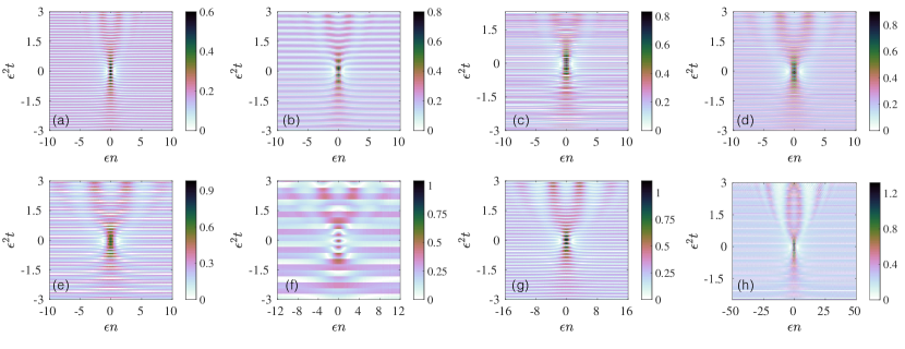
Figure 4: Simulation of Eq. (9) that is initialized with Eq. (17) and Eq. (18) with $A$ given by Eq. (20) with $P_{0}=1$, $\varepsilon=0.5$, $X\in[-40,40]$ and $T\in[-5,5]$. Color intensity corresponds to the strain $|y_{n}|$. The values of the mass ratio parameter are (a) $\rho=0.1$, (b) $\rho=0.2$, (c) $\rho=0.3$, (d) $\rho=0.4$, (e) $\rho=0.5$, (f) $\rho=0.6$, (g) $\rho=0.7$, (h) $\rho=0.9$,

IV Discussion and future directions

In the present study, we have definitively illustrated the potential of phononic lattices to support rogue wave structures. Our preliminary considerations focused on the FPUT lattice as a prototypical example where rogue waves could be excited by using the Peregrine soliton solution of the derived NLS equation as initial data. For sufficiently wide Gaussians, we also found rogue-wave patterns in line with the universality of the gradient catastrophe mechanism suggested by bertola . However, for Peregrine and Gaussian initial data, the formation of the large amplitude structures led eventually to deviations in the FPUT dynamics from the expected predictions of the NLS approximation. While part of the observed discrepancies may be attributed to boundary effects, the predominant reason for this phenomenology is the presence of the modulational instability for the background on top of which the Peregrine structure is formed. We also considered a diatomic granular crystal to demonstrate that rogue wave dynamics is possible in a system that is highly accessible in experiments in a space-time resolved way gc_review . A key challenge in that regard concerns the large scales considered in this paper (where the NLS approximation is valid) leading to large lattices. However, it may be interesting to try relevant ideas in smaller lattices; some studies have considered lattices as large as $N=81$ nodes Boechler2009 , or even $N=188$ nodes in dev . While this paper establishes important first steps for the realization of phononic rogue waves, future theoretical studies should consider further steps in some of these directions; another important one involves the suitable initialization with Peregrine-like initial data, as these lattices permit considerable control e.g. over driving the boundaries, but are less amenable to a distributed initialization over the entire chain. Such topics are presently under consideration and will be reported in future publications.

References

- (1) E. Pelinovsky and C. Kharif (eds.), Extreme Ocean Waves (Springer, NY, 2008).
- (2) C. Kharif, E. Pelinovsky, and A. Slunyaev, Rogue Waves in the Ocean (Springer, NY, 2009).
- (3) A. R. Osborne, Nonlinear Ocean Waves and the Inverse Scattering Transform (Academic Press, Amsterdam, 2010).
- (4) Catherine Sulem and Pierre-Louis Sulem, The Nonlinear Schrödinger Equation: Self-Focusing and Wave Collapse (Springer, NY, 1999)
- (5) D. H. Peregrine, J. Austral. Math. Soc. B 25, 16 (1983).
- (6) D. R. Solli, C. Ropers, P. Koonath, and B. Jalali, Nature 450, 1054 (2007).
- (7) B. Kibler et al., Nature Phys. 6, 790 (2010).
- (8) B. Kibler et al., Sci. Rep. 2, 463 (2012).
- (9) J. M. Dudley, F. Dias, M. Erkintalo, and G. Genty, Nat. Photon. 8, 755 (2014).
- (10) B. Frisquet et al., Sci. Rep. 6, 20785 (2016).
- (11) C. Lecaplain, Ph. Grelu, J. M. Soto-Crespo, and N. Akhmediev, Phys. Rev. Lett. 108, 233901 (2012).
- (12) A. N. Ganshin, V. B. Efimov, G. V. Kolmakov, L. P. Mezhov-Deglin, and P. V. E. McClintock, Phys. Rev. Lett. 101, 065303 (2008).
- (13) A. Chabchoub, N. P. Hoffmann, and N. Akhmediev, Phys. Rev. Lett. 106, 204502 (2011).
- (14) A. Chabchoub, N. Hoffmann, M. Onorato, and N. Akhmediev, Phys. Rev. X 2, 011015 (2012).
- (15) A. Chabchoub and M. Fink, Phys. Rev. Lett. 112, 124101 (2014).
- (16) H. Xia, T. Maimbourg, H. Punzmann, and M. Shats, Phys. Rev. Lett. 109, 114502 (2012).
- (17) M. Shats, H. Punzmann, and H. Xia, Phys. Rev. Lett. 104, 104503 (2010).
- (18) H. Bailung, S. K. Sharma, and Y. Nakamura, Phys. Rev. Lett. 107, 255005 (2011).
- (19) E. G. Charalampidis, J. Cuevas-Maraver, D. J. Frantzeskakis, and P. G. Kevrekidis, Rom. Rep. Phys. 70, 504 (2018).
- (20) Y. Shen, P. G. Kevrekidis, G. P. Veldes, D. J. Frantzeskakis, D. DiMarzio, X. Lan, and V. Radisic, Phys. Rev. E 95, 032223 (2017).
- (21) N. Akhmediev and A. Ankiewicz, Phys. Rev. E 83, 046603 (2011).
- (22) D. Han, M. Westley, and S. Sen, Phys. Rev. E 90, 032904 (2014).
- (23) E. Fermi, J. Pasta, and S. Ulam. Studies in nonlinear problems, I. Los Alamos report, LA 1940, 1955.
- (24) G. Gallavotti, The Fermi–Pasta–Ulam Problem: A Status Report (Springer-Verlag, Berlin, Germany, 2008).
- (25) P. G. Kevrekidis. Nonlinear waves in lattices: Past, present, future. IMA J Appl Math 76, 389-423 (2011).
- (26) V. F. Nesterenko, Dynamics of Heterogeneous Materials (Springer-Verlag, New York, NY, 2001).
- (27) S. Sen, J. Hong, J. Bang, E. Avalos, and R. Doney, Phys. Rep. 462, 21 (2008).
- (28) G. Theocharis, N. Boechler, and C. Daraio, Nonlinear phononic periodic structures and granular crystals, in Acoustic Metamaterials and Phononic Crystals, Springer-Verlag, Berlin, Germany, 2013, 217–251.
- (29) A. F. Vakakis, Analytical methodologies for nonlinear periodic media, in Wave Propagation in Linear and Nonlinear Periodic Media (International Center for Mechanical Sciences (CISM) Courses and Lectures), Springer-Verlag, Berlin, Germany, 2012, 257.
- (30) C. Chong, M. A. Porter, P. G. Kevrekidis, and C. Daraio, J. Phys.: Condens. Matter, 29, 413003 (2017).
- (31) M. A. Porter, P. G. Kevrekidis, and C. Daraio, Physics Today 68, 44 (2015).
- (32) Y. Starosvetsky, K. Jayaprakash, M. A. Hasan, and A. Vakakis, Dynamics and Acoustics of Ordered Granular Media, World Scientific, Singapore, 2017.
- (33) G. Schneider, Appl. Anal. 89, 1523 (2010).
- (34) G. Huang, Z.-P. Shi, and Z. Xu, Phys. Rev. B 47, 14561 (1993).
- (35) G. Huang and B. Hu, Phys. Rev. B 57, 5746 (1998).
- (36) M. Bertola and A. Tovbis, Comm. Pure Appl. Math. 66, 678 (2013).
- (37) A. Tikan, C. Billet, G. El, A. Tovbis, M. Bertola, T. Sylvestre, F. Gustave, S. Randoux, G. Genty, P. Suret, and J.M. Dudley Phys. Rev. Lett. 119, 033901 (2017).
- (38) C. Chong, P. G. Kevrekidis, G. Theocharis, and C. Daraio, Phys. Rev. E 87, 042202 (2013).
- (39) C. Chong, F. Li, J. Yang, M. O. Williams, I. G. Kevrekidis, P. G. Kevrekidis, and C. Daraio, Phys. Rev. E 89, 032924 (2014).
- (40) E. Kim, R. Chaunsali, H. Xu, J. Jaworski, J. Yang, P. G. Kevrekidis, and A. F. Vakakis, Phys. Rev. E 92, 062201 (2015).
- (41) Y. Zhang, D. Pozharskiy, D. M. McFarland, P. G. Kevrekidis, I. G. Kevrekidis, and A. F. Vakakis, Exp. Mech. 57, 505 (2017).
- (42) K. R. Jayaprakash, Y. Starosvetsky, and A. F. Vakakis, Phys. Rev. E 83, 036606 (2011).
- (43) K. R. Jayaprakash, Y. Starosvetsky, A. F. Vakakis, and O. V. Gendelman, J. Nonlinear Sci. 23, 363 (2013).
- (44) N. Boechler, G. Theocharis, S. Job, P. G. Kevrekidis, M. A. Porter, and C. Daraio, Phys. Rev. Lett. 104, 244302 (2010).
- (45) R. Carretero-González, D. Khatri, M.A. Porter, P.G. Kevrekidis, and C. Daraio, Phys. Rev. Lett. 102, 024102 (2009).