Universes without the Weak Force: Astrophysical Processes with Stable Neutrons

Abstract

We investigate a class of universes in which the weak interaction is not in operation. We consider how astrophysical processes are altered in the absence of weak forces, including Big Bang Nucleosynthesis (BBN), galaxy formation, molecular cloud assembly, star formation, and stellar evolution. Without weak interactions, neutrons no longer decay, and the universe emerges from its early epochs with a mixture of protons, neutrons, deuterium, and helium. The baryon-to-photon ratio must be smaller than the canonical value in our universe to allow free nucleons to survive the BBN epoch without being incorporated into heavier nuclei. At later times, the free neutrons readily combine with protons to make deuterium in sufficiently dense parts of the interstellar medium, and provide a power source before they are incorporated into stars. Almost all of the neutrons are incorporated into deuterium nuclei before stars are formed. As a result, stellar evolution proceeds primarily through strong interactions, with deuterium first burning into helium, and then helium fusing into carbon. Low-mass deuterium-burning stars can be long-lived, and higher mass stars can synthesize the heavier elements necessary for life. Although somewhat different from our own, such universes remain potentially habitable.

I Introduction

The fundamental constants that describe the laws of physics appear to have arbitrary values that cannot be explained by current theory. One possible — and partial — explanation is that other universes exist in which the fundamental constants have different values, so that they are drawn from an as-yet-unknown probability distribution. Many authors have argued that significant changes in these constants could render the universe uninhabitable to life as we know it, and as a result our universe appears to be “fine-tuned” for life Barrow and Tipler (1986); Carr and Rees (1979); Carter (1983); Hogan (2000); Rees (2000). On the other hand, recent work suggests that when multiple constants are allowed to vary, large regions of the parameter space that result in habitable universes can be found Adams (2008, 2016); Adams et al. (2015). This paper continues the exploration of alternate possibilities for the fundamental constants with a focus on the weak force.

The strength of the weak interaction is a fundamental part of the standard model of particle physics and represents one parameter that could vary from region to region. The weak interaction governs the rate of radioactive decay, the rate of conversion of hydrogen into helium via the $p(p,\nu_{e}e^{+}){\rm D}$ stage of the $pp$-chain in low-mass stars, and the cross section for neutrino interactions. The latter two effects are crucial to determining whether or not a universe can produce life. If the weak force is too weak, or absent altogether, long-lived stars fueled by weak reactions could not exist. In the absence of weak interactions, helium can still be synthesized through strong interactions during Big Bang Nucleosynthesis (BBN), as free neutrons are present, but helium production is suppressed in stellar interiors (which do not have neutrons). Once synthesized, helium can later fuse into heavier elements via the triple alpha process in sufficiently massive stars. However, without neutrino interactions, core-collapse supernova will fail to explode and will simply collapse to a degenerate remnant, thereby hampering the dispersal of heavy elements.

These effects would appear to compromise the habitability of universes where the weak force is significantly weaker than in our own. However, this standard argument has been challenged with the concept of a “weakless universe” Harnik et al. (2006), namely, a universe without any weak interaction at all. Neutrons would be stable in such a universe, and would therefore most likely have an equal abundance to protons. A universe with the same baryon density as ours would convert virtually all baryons to helium during BBN, leaving behind no free protons (no hydrogen to make water). However, if the baryon density is lower (more properly the baryon-to-photon ratio $\eta$), significant amounts of protons and deuterium can survive the BBN epoch Harnik et al. (2006) and would be available later for deuterium burning in stars (which takes place through the strong interaction). Note that stars in such a weakless universe can also produce heavier elements by strong reactions. Although core-collapse supernova might not function, at least not in the same manner as in our universe, these heavy elements could still be dispersed by Type Ia supernova and classical novae, allowing the possibility of planet formation and life.

The opposite case, where the weak interaction is significantly stronger than in our universe, would resemble our universe more closely. A stronger weak interaction increases the rate of radioactive decay, most notably the neutron lifetime, but it does not affect the stability of stable nuclei, which is governed primarily by the strong interaction. If the neutron lifetime is less than 30 seconds, BBN is suppressed because most neutrons decay before BBN begins. However, this complication is not an impediment because stars in this all-hydrogen universe will be more efficient at converting hydrogen to helium. In addition, core-collapse supernovae will be more efficient at dispersing heavy elements due to the larger neutrino interaction cross sections. The primary concern would be the shortened lifetimes of these more efficient stars. (Note that if the weak interaction is strong enough to approach the strength of the electromagnetic interaction, non-linear effects will likely render these concerns moot.)

In this paper, we update and expand upon this idea of a weakless universe in Refs. Clavelli and White (2006); Gedalia et al. (2011); Giudice et al. (2012), and in particular Ref. Harnik et al. (2006). An important parameter in this problem is the baryon-to-photon ratio $\eta$, which impacts the composition of the universe after BBN. For the value in our universe, BBN with an equal amount of neutrons and protons would result in a composition where the ⁴He abundance is greater than $90\%$. The high abundance of $\,{}^{4}\textnormal{He}$ yields short-lived stars and is problematic for the development of life. For a judicious choice of $\eta$, however, BBN can result in a richer composition with large fractions of deuterium, free protons, and free neutrons. We determine the range of $\eta$ for which weakless universes could support life, using models of galaxy formation, star formation, and subsequent stellar evolution.

One crucial issue not addressed in the original proposal Harnik et al. (2006) is the abundance of free neutrons left over from BBN, which is comparable to the abundance of free protons. These neutrons can capture onto protons at zero temperature, forming deuterium via the $n(p,\gamma){\rm D}$ reaction. As a result, nuclear fusion can occur in the interstellar medium and could potentially halt the collapse of a gas cloud. This paper considers the effects of neutron capture reactions on four scales of formation: [A] from the intergalactic medium down to the size scale of galaxies; [B] from the neutral interstellar medium (ISM) to the formation of giant molecular clouds; [C] from the cloud to molecular cloud cores – the sites of individual star formation events; and finally [D] from the cloud cores to the production of protostars themselves. Neutron fusion becomes significant during the latter stages of this hierarchy, and most of the free neutrons are processed into deuterium before the onset of stellar nuclear burning. Although gas cooling is delayed, these processes do not disrupt star formation entirely.

We next consider stellar evolution and nuclear burning in a weakless universe and the chemical evolution of the universe through successive generations of stars. Long-lived stars can exist in a weakless universe if the deuterium abundance is high enough for deuterium fusion to continue on Gyr timescales. With the main sources of heavy element dispersal being red giant winds and Type Ia supernovae, the composition of the interstellar medium will be different from our universe, relatively enriched in carbon and iron peak elements and depleted in oxygen. A low oxygen abundance could cause a dearth of water which would impose a problem to life – assuming water is an essential ingredient to life like it is on our planet. However, later generations of stars will undergo different reactions that will likely mitigate this problem.

Iron peak elements in the ISM will capture an excess of free neutrons, allowing stars to form with a small excess of protons, which can then form oxygen via the reaction ${}^{12}\textnormal{C}(2p,\gamma){}^{14}{\rm O}$. Similar reactions may lead to a deficit of nitrogen and an excess of neon compared with our universe, and likewise, the lack of core-collapse supernovae will likely lead to a deficit of non-alpha-process elements. However, the effect on the chemical evolution of the weakless universe is neither negligible nor dominant, and the necessary elements for both planet formation and organic chemistry will still be present, implying that such a universe could still be hospitable to life.

The organization of this paper is as follows. Section II details the outcome of BBN in universes with a range of $\eta$ and neutron-to-proton ratios. We examine the impact of weakless physics on: galaxy formation in Sec. III; the ISM in Sec. IV; and stellar evolution in Sec. V. Section VI contains our study of the habitability of the weakless universe. We summarize and discuss our results in Sec. VII. Throughout this paper, we use cgs units with the exception of BBN in Sec. II. We use natural units in Sec. II to be consistent with the BBN literature.

II Big Bang Nucleosynthesis

II.1 Standard versus weakless BBN

In this section, we give a brief overview of the role the weak interaction plays in Standard BBN (SBBN) and then discuss the modifications to SBBN in a weakless universe. We will use the ratio of neutrons to protons (denoted the $n/p$ ratio) extensively throughout this work

$$n/p\equiv\frac{n_{n}}{n_{p}}.$$ (1)

Note that the number densities $n_{i}$ in Eq. (1) are the total particle number densities (free particles and nucleons bound in nuclei) and not solely the free particle number densities. Reference Hayashi (1950) showed that $n/p$ would evolve due to six weak reactions during primordial nucleosynthesis. We schematically write the six reactions as

$$\nu_{e}+n \leftrightarrow p+e^{-},$$ (2)

$$e^{+}+n \leftrightarrow p+\overline{\nu}_{e},$$ (3)

$$n \leftrightarrow p+e^{-}+\overline{\nu}_{e}.$$ (4)

and colloquially refer to them as the $n\leftrightarrow p$ rates. In the approximation that the nucleon rest masses are much heavier than both the neutrino and electron masses, Ref. Grohs and Fuller (2016) gives the prescription for calculating the rates for each of the six reactions listed in Eqs. 2 – 4. At high temperature $T$, the weak interaction rates are fast and maintain the $n/p$ ratio in weak equilibrium as a function of $T$

$$n/p\,(T)=\exp\left(\frac{-\delta m_{np}+\mu_{e^{-}}-\mu_{\nu_{e}}}{T}\right),$$ (5)

where $\delta m_{np}=1.293\,\,{\rm MeV}$ is the mass difference between a neutron and proton, $\mu_{e^{-}}$ is the chemical potential of the electrons, and $\mu_{\nu_{e}}$ is the chemical potential of the electron neutrinos. In SBBN, the chemical potentials of the electron and electron neutrino are small and so the mass term dominates. Therefore, $n/p\simeq 1$ at high temperature. Figure 6 of Ref. Grohs and Fuller (2016) shows how $n/p$ initially follows an equilibrium track for temperatures above $1\,\,{\rm MeV}$, and diverges from equilibrium at lower temperature. Free neutron decay [the forward process in Eq. (4)] would eventually transmute all neutrons into protons if there were no other nuclear processes. $n/p$ would go to zero and the universe would emerge from BBN with a pure ${}^{1}\textnormal{H}$ composition. Such a scenario does not transpire as a chain of reactions assembles free protons and neutrons into $\,{}^{4}\textnormal{He}$ and some other low atomic mass nuclides. Nuclear freeze-out of $\,{}^{4}\textnormal{He}$ occurs when the temperature has reached $T\sim 100\,\,{\rm keV}$ and $n/p\sim 1/7$.

In a weakless universe, there are no weak interactions and Eqs. (2) – (4) do not apply. This implies that neutrons are stable to decay. The neutron to proton ratio is set at a high temperature and is a function of the ratio of up quarks to down quarks, $u/d$

$$n/p=\frac{2-u/d}{2u/d-1}.$$ (6)

$u/d$ ranges from $1/2$ for a pure neutron universe to $2$ for a pure proton universe. Assuming baryon number conservation, $n/p$ is fixed and does not evolve. Weakless BBN (wBBN) proceeds with a fixed $n/p$ ratio. If there are multiple families of quarks with nonzero densities, then there would be other hadrons present. We do not consider such scenarios in this work.

II.2 Description of calculations

We employ the code burst Grohs et al. (2015) to do both SBBN and wBBN calculations. burst is based off of the work in Refs. Wagoner et al. (1967) and Smith et al. (1993). In a SBBN calculation, there are four sets of quantities to evolve as a function of time. There are three thermodynamic variables: the plasma temperature $T$; the scale factor $a$; and the electron-degeneracy parameter $\phi_{e}$ where

$$\phi_{e}\equiv\frac{\mu_{e^{-}}}{T}.$$ (7)

All thermodynamic quantities of the plasma, such as energy density and pressure, are functions of $T$, $a$, and $\phi_{e}$. The last set of evolution quantities are the abundances $Y_{i}$. Abundances are related to the mass fractions $X_{i}$ via

$$Y_{i}=\frac{X_{i}}{A_{i}},$$ (8)

where $A_{i}$ is the atomic mass number for species $i$. To compare SBBN and wBBN calculations, we will employ a network of nine nuclides which include all bound nuclides up to mass number $A=7$. The nuclear reaction network includes 34 strong, electromagnetic, and weak interactions from Refs. Smith et al. (1993) and Caughlan and Fowler (1988). For more precise calculations of SBBN, one can evolve the neutrino spectra as they go out of equilibrium which can lead to changes at the $1\%$ level Grohs et al. (2016). The present work does not require this level of precision, so we always assume neutrinos are in a Fermi-Dirac distribution with zero chemical potential and a temperature given by the comoving temperature parameter $T_{\textnormal{cm}}$ as a function of scale factor $a$

$$T_{\textnormal{cm}}(a)\equiv T_{\rm in}\frac{a_{\rm in}}{a}.$$ (9)

The subscript “in” on the temperature and scale factor symbols denotes an initial epoch when the neutrinos are in thermal equilibrium with the electromagnetic components of the plasma. We must use $T_{\textnormal{cm}}$ because it is manifestly different from $T$ and has ramifications on the $n/p$ ratio Grohs and Fuller (2017).

A wBBN calculation proceeds in the same way as a SBBN one. We evolve $T$, $a$, $\phi_{e}$, and the nine nuclides as a function of time. We maintain all strong and electromagnetic cross sections unaltered from SBBN. There are two key differences between wBBN and SBBN. In a weakless universe, there are no weak nuclear interactions. We remove the $n\leftrightarrow p$ rates, i.e., Eqs. (2) – (4), and any other $\beta$-decay rates, most notably that of the three-nucleon hydrogen isotope tritium (denoted as ${\rm T}$), ${\rm T}\rightarrow\,^{3}\textnormal{He}+e^{-}+\overline{\nu}_{e}$. Tritium has a mean lifetime $\tau_{3}\sim 20\,{\rm years}$ and will not decay into $\,{}^{3}\textnormal{He}$ until well after SBBN concludes. If doing precision SBBN calculations, we would add the abundance of ${\rm T}$ to that of $\,{}^{3}\textnormal{He}$ to compare to observation Bania et al. (2002). In a weakless universe however, the difference in atomic number between T and $\,{}^{3}\textnormal{He}$ could be important in the initial stages of stellar evolution. As a result, we delineate the freeze-out ${\rm T}$ and $\,{}^{3}\textnormal{He}$ abundances in order to use them in our stellar calculations.

The other difference between SBBN and wBBN is the existence of neutrinos. Our model of SBBN in Ref. Grohs et al. (2015) assumes that neutrinos only interact via the weak interaction and gravity. We do not know the mechanism which populates the neutrino states at early times in our universe. In this work, we assume that if there is no weak interaction, then there would be no relic neutrino seas. We note that if there were neutrinos in a weakless universe, then the neutrino energy states would not necessarily be thermally populated. Alternatively, one could consider the Cosmic Microwave Background (CMB) observable $N_{\textnormal{eff}}$. $N_{\textnormal{eff}}$ is the “effective number of neutrino species” [see Eq. (3.11) in Ref. Carlstrom and et al. (2016)]. In our universe, $N_{\textnormal{eff}}\sim 3$ for the three flavors of neutrino species Planck Collaboration et al. (2016). In a weakless universe where neutrinos were present, $N_{\textnormal{eff}}$ would most likely be smaller than 3. The exact number would depend on the mechanism which created the neutrinos. The neutrinos would behave as a dark radiation component Mukohyama (2000) and wBBN would proceed with an expansion rate different than SBBN. For the wBBN calculations in this work, $N_{\textnormal{eff}}=0$.

II.3 Mass fraction evolution

In this section we discuss the evolution of the mass fractions as a function of the $T_{\textnormal{cm}}$ variable from Eq. (9). For our model of SBBN, the baryon number is the only cosmological input. We do not consider other cosmological inputs such as $N_{\textnormal{eff}}$ or neutrino chemical potentials. There are many equivalent ways to represent baryon number in BBN. We adopt the nomenclature of Ref. Smith et al. (1993) and use the baryon-to-photon ratio $\eta$

$$\eta\equiv\frac{n_{b}}{n_{\gamma}},$$ (10)

where $n_{b}$ and $n_{\gamma}$ are the proper number densities of baryons and photons, respectively. Based on the strict definition in Eq. (10), $\eta$ decreases as electrons and positrons annihilate to become photons for $T\lesssim 100\,{\rm keV}$. Therefore, we will refer to numerical values of $\eta$ after the epoch of electron-positron annihilation. In wBBN, $\eta$ and the $n/p$ ratio are both inputs. When comparing SBBN to wBBN, we will use the same value of $\eta$. There is no way to compare SBBN to wBBN using the same $n/p$ ratio as $n/p$ evolves in SBBN according to the $n\leftrightarrow p$ rates schematically shown in Eqs. (2) – (4). We will pick a value of the $n/p$ ratio to elucidate specific points on how wBBN differs from SBBN.

Figures 1 and 2 show mass fractions versus $T_{\textnormal{cm}}$ in a number of BBN cases. Solid lines are from a SBBN calculation with an evolving $n/p$ ratio and dashed lines from a wBBN calculation with a constant $n/p$ ratio. Both calculations, for a given figure, use the same value of $\eta$. For ease in reading, we only plot the mass fractions of free neutrons ($n$), free protons ($p$), deuterium (${\rm D}$), tritium (${\rm T}$), helium-3 ($\,{}^{3}\textnormal{He}$), and helium-4 ($\,{}^{4}\textnormal{He}$). We note that the mass fractions of ${}^{6}\textnormal{Li}$, ${}^{7}\textnormal{Li}$, and ${}^{7}\textnormal{Be}$ are all subsidiary to that of the hydrogen and helium isotopes in both SBBN and wBBN. We do not include other possibly stable isotopes in a weakless universe, i.e., ${}^{6}{\rm He}$.

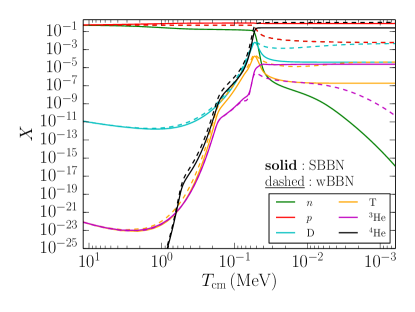
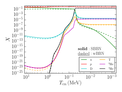
Figure 1: Mass fractions, $X$, as a function of $T_{\textnormal{cm}}$. Each color represents a different isotope. (Top) Solid lines are a SBBN calculation, and dashed lines are a wBBN calculation where $n/p=1$. The dashed green line for $n$ is coincident with the dashed red line for $p$. $\eta=6.075\times 10^{-10}$ for both calculations. (Bottom) Same as the top panel except $n/p=0.14$ for the wBBN calculation.

Figure 1 uses $\eta=6.075\times 10^{-10}$ which is consistent with the value in our universe Planck Collaboration et al. (2016). $n/p=1$ for the wBBN calculation in the top panel. At high temperatures, the abundances are in Nuclear Statistical Equilibrium (NSE). NSE abundances are functions of plasma temperature, $\eta$, $X_{n}$, $X_{p}$, and nuclear properties Burbidge et al. (1957). The mass fractions of ${\rm D}$, ${\rm T}$, and $\,{}^{3}\textnormal{He}$ are all following NSE tracks above $T\gtrsim 1\,{\rm MeV}$ ($\,{}^{4}\textnormal{He}$ also follows a NSE track below the scale of the vertical axis). For temperatures $T>\delta m_{np}$ in a SBBN calculation, Eq. (5) shows that $n/p\sim 1$, implying that the SBBN and wBBN scenarios have the same conditions for NSE. As a result, the mass fractions evolve identically for both SBBN and wBBN at high temperatures in the top panel. Although the mass fractions remain in NSE, the SBBN curves begin to diverge from the wBBN curves once $T$ becomes comparable to $\delta m_{np}$. At even lower temperatures, $n/p$ for SBBN is well below unity and the mass fractions diverge for the two scenarios. Note that the red dashed curve ($X_{p}$ in wBBN) is on top of the green dashed curve ($X_{n}$ in wBBN) in the top panel in Fig. 1. The wBBN mass fractions for $n$, $p$, and ${\rm D}$ have frozen out at the end of the horizontal plotting axis. Although neutrons and protons can interact to form deuterons, the baryon density is so low that all three mass fractions have frozen out at roughly the $1\%$ level.

For SBBN at $\eta=6.075\times 10^{-10}$, $\,{}^{4}\textnormal{He}$ freezes-out with a mass fraction $X_{\,{}^{4}\textnormal{He}}\equiv Y_{P}\simeq 0.25$, where we adopt the cosmological notation of $Y_{P}$ to denote the mass fraction of $\,{}^{4}\textnormal{He}$. The top panel of Fig. 1 shows that the number of baryons in ${\rm D}$ and $\,{}^{3}\textnormal{He}$ is only a few in $10^{5}$, implying that the vast majority of neutrons are in $\,{}^{4}\textnormal{He}$ nuclei. Therefore, $n/p\simeq 1/7=0.14$ at the conclusion of SBBN. The bottom panel of Fig. 1 shows the same SBBN calculation as the top panel, but the wBBN calculation now has $n/p=0.14$. In the NSE regime at high temperatures, there is a clear difference between the SBBN and wBBN calculations. As the temperature decreases and the $n/p$ ratios converge to one another for the two scenarios, the abundances begin to come into agreement, especially for $p$ and $\,{}^{4}\textnormal{He}$.

Nuclear reactions which involve the capture of a neutron are not subject to the Coulomb repulsion unavoidable in proton capture reactions. At low temperatures, neutrons can continue to capture on heavier nuclei or free protons. It is possible for BBN to occur over a long period if free neutrons are present and the proper baryon number density is large. For the wBBN calculation in the top panel of Fig. 1, there is a preponderance of free neutrons at $T_{\textnormal{cm}}\simeq 10\,{\rm keV}$, although the number density of baryons is low enough that there is no late-time rise in ${\rm D}$. However, the flux of neutrons is large compared to the number of $\,{}^{3}\textnormal{He}$ targets. The principal reactions which utilize neutrons and $\,{}^{3}\textnormal{He}$ nuclei as reactants, namely $\,{}^{3}\textnormal{He}(n,p){\rm T}$ and $\,{}^{3}\textnormal{He}(n,\gamma)\,^{4}\textnormal{He}$, have not frozen-out at the end of the plotting axis. As a result, the $\,{}^{3}\textnormal{He}$ mass fraction continues to decrease at the end of the simulation. Similarly, the flux of neutrons compared to ${}^{6}\textnormal{Li}$, ${}^{7}\textnormal{Li}$, and ${}^{7}\textnormal{Be}$ targets is also large in the weakless scenario. If we had plotted the mass fractions of the Li and Be isotopes, they would also be decreasing at the end of the horizontal plotting axis in much the same manner as the mass fraction for $\,{}^{3}\textnormal{He}$ does. We verified our hypotheses by extending the wBBN calculation down to temperature of $T=100\,{\rm eV}$. However, our library for the integrated cross sections (based off of that in Ref. Smith et al. (1993)) is not accurate at such low temperatures. Furthermore, the error in not finishing the wBBN calculation would be small as the mass fractions of $\,{}^{3}\textnormal{He}$ and the heavier isotopes are orders of magnitude smaller than the more abundant species. As we consider the composition of the later weakless universe, we will take the mass fractions from wBBN at the $T\sim 1\,{\rm keV}$ epoch and ignore the small error present in $\,{}^{3}\textnormal{He}$.

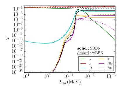
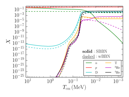
Figure 2: Mass fractions, $X$, as a function of $T_{\textnormal{cm}}$. Each color represents a different isotope. (Top) Solid lines are a SBBN calculation, and dashed lines are a weakless calculation where $n/p=1$. The dashed green line for $n$ is coincident with the dashed red line for $p$. $\eta=4.0\times 10^{-12}$ for both calculations. (Bottom) Same as the top panel except $n/p=0.026$ for the wBBN calculation.

In Fig. 2, we use a value of $\eta=4.0\times 10^{-12}$. This specific value is in line with the value chosen in Ref. Harnik et al. (2006). The top panel of Fig. 2 shows the evolution of the mass fractions for SBBN and wBBN with $n/p=1$. For SBBN, the mass fractions of ${\rm D}$, ${\rm T}$, and $\,{}^{3}\textnormal{He}$ are all increased over the freeze-out mass fractions when $\eta=6.075\times 10^{-10}$ in Fig. 1. $\,{}^{4}\textnormal{He}$ is significantly reduced for the low value of $\eta$ in Fig. 2. Conversely, in wBBN there are roughly equal amounts of $n$, $p$, ${\rm D}$, and $\,{}^{4}\textnormal{He}$. The freeze-out mass fractions are in close agreement with Fig. [1] in Ref. Harnik et al. (2006). As compared to the top panel of Fig. 1, neutrons are not predominantly incorporated into $\,{}^{4}\textnormal{He}$ nuclei for the lower value of $\eta$. In both SBBN and wBBN, the ${\rm D}$ mass fraction is comparable to that of $\,{}^{4}\textnormal{He}$. SBBN makes less $\,{}^{4}\textnormal{He}$ (and less ${\rm D}$) as the $n/p$ ratio evolves to 0.026.

The bottom panel of Fig. 2 is identical to the top panel except we run wBBN with $n/p=0.026$. Although the $n/p$ ratios are identical between SBBN and wBBN, the final freeze-out mass fractions of ${\rm D}$ and $\,{}^{4}\textnormal{He}$ differ. Furthermore, in the weakless scenario, there is a larger mass fraction of ${\rm D}$ as compared to $\,{}^{4}\textnormal{He}$. With fewer neutrons, the NSE abundances are lower. We observe this by using the top and bottom panels of Fig. 2 to compare the locations of the dashed lines of ${\rm T}$ and $\,{}^{4}\textnormal{He}$ with respect to the solid SBBN lines. The initial conditions for out-of-equilibrium nucleosynthesis occur when the $n/p$ ratio is still evolving in SBBN, i.e., $n/p>0.026$ when the mass fractions go out of equilibrium. As a result, the sum of $X_{\rm D}$ and $Y_{P}$ is larger in SBBN than wBBN. For the $n/p$ ratios to be equal at freeze-out, the deficit of neutrons in wBBN must be incorporated into a different nuclide. Indeed, the bottom panel of Fig. 2 shows a mass fraction of free neutrons on order of $1\%$. This is a key difference of SBBN compared to wBBN which was absent in Fig. 1: identical $n/p$ ratios at freeze-out do not imply identical mass fractions of ${\rm D}$ and $\,{}^{4}\textnormal{He}$. If the baryon number is low enough, out-of-equilibrium nucleosynthesis begins during weak freeze-out. The $n/p$ ratio alone is not enough to predict the final mass fractions of $\,{}^{4}\textnormal{He}$.

To conclude this section, we note neither SBBN nor wBBN possesses ${\rm D}$ and ${\rm T}$ peaks in Fig. 2. The peaks are quite visible in the bottom panel of Fig. 1 at $T_{\textnormal{cm}}\sim 50\,{\rm keV}$ for both SBBN and wBBN. The peaks stem from synthesis of ${\rm D}$ and ${\rm T}$ into larger nuclei, most notably $\,{}^{4}\textnormal{He}$, and no production channels of equivalent strength. For the lower value of $\eta$, the nuclear reaction rates freeze-out at an earlier time and the mass fractions plateau.

II.4 Parameter space scan

The previous section detailed a comparison between SBBN and wBBN at various values of $\eta$. In this subsection, we explore the $n/p$ versus $\eta$ parameter space of wBBN. We cannot directly compare with SBBN because there is no dual parameter space for cosmological inputs [see Fig. (2) in Ref. Adams et al. (2017) for SBBN mass fractions as a function of $\eta$]. As an alternative, we place a red star on the contour plots at the values $\eta=6.075\times 10^{-10}$ and $n/p=0.14$ of our universe. The red star comes from a simulation that models our universe with the weak interaction, namely the SBBN calculation in Fig. 1. $n/p$ changes with time in such a scenario. In addition, our universe contains neutrino energy density so the Hubble expansion rate is different. We emphasize that the red star is only for illustrative purposes and does not belong to the class of weakless universes. It is only meant as a guide and not for direct comparison.

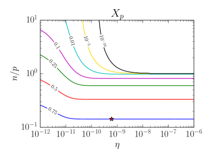
Figure 3: The neutron-to-proton ratio, $n/p$, versus the baryon-to-photon ratio, $\eta$, at contours of constant $p$ mass fraction. In a weakless universe, $n/p$ is fixed at the start of BBN and does not evolve through nuclear freeze-out. In our universe, weak interactions change $n/p$ until $\,{}^{4}\textnormal{He}$ formation when $n/p\approx 1/7$. The red star indicates the point in parameter space where $n/p$ terminates its evolution in our universe. This point should only be taken for illustrative purposes and not labeled a member of the weakless class of universes.

Figure 3 shows contours of constant $p$ mass fraction in the $n/p\,$ – $\eta$ plane. The red star is located close to the $75\%$ contour, which is in agreement with the value from SBBN as seen on the bottom panel of Fig. 1. For the range of $\eta$ plotted, a significant fraction of the baryons are free protons if $n/p$ is below unity. Once $n/p$ becomes larger than unity, few free protons remain. The isospin mirror of Fig. 3 is Fig. 4: contours of constant $X_{n}$ in the $n/p\,$ – $\eta$ plane. For $n/p$ above unity, there exists a significant fraction of free neutrons. Conversely, for $n/p$ below unity, few free neutrons remain.

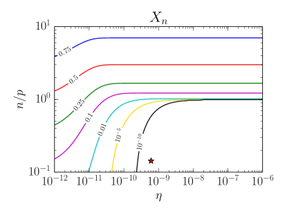
Figure 4: $n/p$ versus $\eta$ at contours of constant $n$ mass fraction. The red star indicates the point in parameter space where $n/p$ terminates its evolution in our universe.

Figures 3 and 4 show a remarkable degree of symmetry about the line $n/p=1$. The symmetry is broken, albeit slightly, in the mass fraction of ${\rm D}$. Figure 5 shows contours of constant $X_{\rm D}$ in the $n/p\,$ – $\eta$ plane. At constant $\eta$, the mass fraction of ${\rm D}$ increase as $n/p$ approaches unity from either direction. The rate of increase is larger as $n/p$ decreases towards unity. This is only evident for large $\eta$ in Fig. 5. The contours of $X_{\rm D}$ at $10^{-5}$ and $10^{-10}$ are closer in the parameter space for $n/p>1$. The value of the contours indicates that the degree of asymmetry is small – a few parts in $10^{5}$.

The red star in Fig. 5 is located on the $X_{\rm D}=2.7\times 10^{-5}$ contour. For comparison, the ${\rm D}$ mass fraction of SBBN is $4.0\times 10^{-5}$. wBBN is able to produce a large mass fraction of ${\rm D}$. The largest mass fraction of ${\rm D}$ is $X_{\rm D}=0.14$ at $n/p=1$ and $\eta=5\times 10^{-12}$.

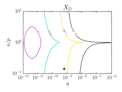
Figure 5: $n/p$ versus $\eta$ at contours of constant ${\rm D}$ mass fraction. The red star indicates the point in parameter space where $n/p$ terminates its evolution in our universe.

The symmetry about $n/p=1$ is restored in Fig. 6: contours of constant $Y_{P}$ in the $n/p\,$ – $\eta$ plane. For the parameter space shown in Fig. 6, the smallest value of $Y_{P}$ is $\sim 7\times 10^{-3}$. This value occurs for small $\eta$ and either large or small $n/p$. The mass fraction value is above our asymmetry limit of $10^{-5}$, so we cannot detect any visible asymmetry in Fig. 6. For small $\eta$, Fig. 6 shows that not all neutrons are incorporated into $\,{}^{4}\textnormal{He}$ nuclei. In fact, the mass fraction of ${\rm D}$ is larger than that of $\,{}^{4}\textnormal{He}$ for a certain range of $\eta$ if $n/p=1$. Furthermore, Fig. 4 shows that most neutrons are free at small $\eta$. For large $\eta$, the mass fraction of $\,{}^{4}\textnormal{He}$ is independent of $\eta$ in the range of $n/p$ we employ in Fig. 6. The contours of constant mass fraction are symmetrical about $n/p=1$ and horizontal. We can succinctly capture the relationship between the mass fraction of $\,{}^{4}\textnormal{He}$ and $n/p$ in this range

$$Y_{P}\simeq 2\,\frac{\min(1,n/p)}{1+n/p}.$$ (11)

If $n/p<1$, Eq. (11) reduces to the familiar $Y_{P}=2(n/p)/(1+n/p)$ Kolb and Turner (1990). Finally, we note that the location of the contours in Fig. 6 (or, more specifically, the rounded ends at low $\eta$) depends on the nuclear reaction rates versus the Hubble expansion rate. We do not include neutrinos or any other form of dark radiation in our model of wBBN. If we had, that would increase the Hubble rate and decrease $Y_{P}$. The result would be a shift of the contours in Fig. 6 in the horizontal direction towards higher $\eta$. There would be no change in the vertical direction of Fig. 6 at the level of precision presented in the parameter space.

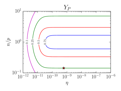
Figure 6: $n/p$ versus $\eta$ at contours of constant $Y_{P}$, the $\,{}^{4}\textnormal{He}$ mass fraction. The red star indicates the point in parameter space where $n/p$ terminates its evolution in our universe.

Table 1 gives the freeze-out mass fractions at numerous values of $\eta$ which we will use in sections III – V. $n/p=1$ for all values of $\eta$. It appears that the ${\rm D}$ mass fraction gets closer to the $n$ and $p$ mass fractions for increasing $\eta$. For $n/p=1$, ${\rm D}$ gets closest to $n$ when $\eta\simeq 10^{-7}$ at a value $X_{\rm D}/X_{n}=0.95$. ${\rm D}$ gets closest to $p$ when $\eta\simeq 5\times 10^{-8}$ at a value $X_{\rm D}/X_{p}=0.86$. The $\,{}^{3}\textnormal{He}$ mass fraction is much lower than the mass fractions for the other nuclides, as explained in Figs. 1 and 2 by the lack of a Coulomb barrier in neutron capture. By the same logic, Table 1 shows a slight excess of the $p$ mass fraction over that of free neutrons even though the universe is isospin symmetric, i.e., $n/p=1$. This is due to the high reactivity of neutrons, or equivalently, a Coulomb barrier in proton capture.

$\eta$		$10^{-11}$	$10^{-10}$	$10^{-9}$
$n$		$0.2136$	$3.420\times 10^{-2}$	$3.535\times 10^{-3}$
$p$		$0.2139$	$3.428\times 10^{-2}$	$3.545\times 10^{-3}$
${\rm D}$		$0.1197$	$2.615\times 10^{-2}$	$2.766\times 10^{-3}$
${\rm T}$		$9.764\times 10^{-4}$	$2.320\times 10^{-4}$	$2.469\times 10^{-5}$
${{}^{3}}\textnormal{He}$		$8.844\times 10^{-10}$	$2.605\times 10^{-10}$	$2.819\times 10^{-11}$
$\,{}^{4}\textnormal{He}$		$0.4518$	$0.9051$	$0.9901$

Table 1: Mass fractions at different values of $\eta$. All values for $n/p=1$.

III Galaxy Formation

This section considers how nuclear reactions involving free neutrons can potentially affect the galaxy formation process. Here we assume that structure formation involves processes that are analogous to those acting in our universe. Without weak interactions, a universe can in principle still produce dark matter Harnik et al. (2006). In this case, the timing of structure formation would remain the same, and this is the case considered here.

For completeness we note that even in the absence of dark matter, a purely baryonic universe can produce structure. In the present context, however, the baryon-to-photon ratio $\eta$ must be smaller due to BBN constraints (see Sec. II.4) so that the epoch of matter domination occurs at lower redshift. As a result, galaxy formation takes place at later epochs when the universe is more diffuse, so that galaxies are less dense for a fixed value of the amplitude $Q$ of density fluctuations. For the particular value $Q=10^{-5}$ realized in our universe, the resulting densities of galaxies could be so low that baryons have difficulty cooling and condensing Tegmark and Rees (1998); Tegmark et al. (2006). This issue can be alleviated with larger values of the fluctuation amplitude $Q$ Tegmark et al. (2006); Adams et al. (2015). With no dark matter (which has $\sim 6$ times the density of baryons in our universe) and lower $\eta$ (by a factor of $\sim 50$), the total matter density is smaller by a factor of $\sim 300$. The corresponding value of the fluctuation amplitude $Q\sim 3\times 10^{-3}$.

III.1 Properties of Dark Matter Halos

Simulations of structure formation show that dark matter halos asymptotically approach a nearly universal form. The density profile of the halo is thus taken to be a Hernquist profile of the form

$$\rho(r)={\rho_{0}\over\xi(1+\xi)^{3}}\,,$$ (12)

where the dimensionless coordinate $\xi$ is defined via

$$\xi={r\over r_{0}}\,.$$ (13)

Note that we use a slightly steeper power-law for the density distribution ($\rho\sim\xi^{-4}$ for $\xi\gg 1$) compared to the often-used NFW profile Navarro et al. (1997) ($\rho\sim\xi^{-3}$). Although only the inner part of the potential well matters for the considerations of this paper, we use the form (12) because it has a finite mass and because numerical simulations show that halo density profiles become steeper at later epochs Busha et al. (2005, 2007). Given the form of equation (12), the corresponding potential and enclosed mass have the forms

$$\Psi={\Psi_{0}\over 1+\xi}\qquad{\rm and}\qquad M(r)=M_{T}\left({\xi\over 1+\xi}\right)^{2}\,.$$ (14)

We can take $\rho_{0}$ and $r_{0}$ to be the defining parameters of the halo. The scale $\Psi_{0}$ for the potential and the total mass $M_{T}$ are then given by

$$\Psi_{0}=2\pi G\rho_{0}r_{0}^{2}\qquad{\rm and}\qquad M_{T}=2\pi\rho_{0}r_{0}^{3}\,.$$ (15)

For the example of the Milky Way galaxy, we can model the halo with a profile of the form given by equation (12) if we take the scale length $r_{0}$ = 65 kpc and the density scale $\rho_{0}$ = $10^{-25}$ g cm^-3 (see Ref. Adams and Bloch (2005) and references therein).

III.2 Hydrostatic Equilibrium

In order to assess the possible effects of nuclear reactions on galaxy formation, we need to determine the temperature and density distributions of the baryonic gas. We start with an order of magnitude estimate: the usual assumption is that dark matter collapses first, and then gas falls into the dark matter halo. The collapse of the gaseous component and subsequent shocks heat up the material to a temperature given by

$$3kT={GMm_{\rm p}\over r}\,,$$ (16)

where $M=M(r)$ is the enclosed mass of the dark matter halo at radius $r$. For the galaxy profiles considered here, this expression becomes

$$3kT={GM_{T}m_{\rm p}\over r_{0}}{\xi\over(1+\xi)^{2}}\,.$$ (17)

For the Milky Way values, the benchmark temperature scale is given by

$$T={GM_{T}m_{\rm p}\over 3kr_{0}}\approx 2.7\times 10^{6}{\rm K}\,.$$ (18)

This estimate is approximate and does not require that the gaseous density and temperature profiles approach an equilibrium condition. We thus generalize the treatment in the following discussion.

For a given dark matter halo, we can determine the density and temperature profile of the gas under the assumptions that: (1) the dark matter halo dominates the gravity of the system; (2) the gas can be considered in hydrostatic equilibrium; and (3) the equation of state for the gas is polytropic

$$P=K\rho^{\Gamma}\equiv K\rho^{1+1/n}\,,$$ (19)

where $n$ is the usual polytropic index and $K$ is a scaling constant. Hydrostatic equilibrium thus implies

$$K\Gamma\rho^{\Gamma-2}{d\rho\over d\xi}=-{\Psi_{0}\over(1+\xi)^{2}}\,,$$ (20)

so that the density profile has the form

$$\rho(\xi)=\left[{(\Gamma-1)\Psi_{0}\over K\Gamma}\right]^{1/(\Gamma-1)}(1+\xi)^{-1/(\Gamma-1)}\,.$$ (21)

To fix ideas, consider the standard case of an adiabatic equation of state for a monoatomic gas, where $\Gamma=5/3$. The density profile then becomes

$$\rho(\xi)=\left[{2\Psi_{0}\over 5K}\right]^{3/2}(1+\xi)^{-3/2}\equiv\rho_{X}(1+\xi)^{-3/2}\,,$$ (22)

where the second equality defines a benchmark density scale. The total mass in baryons is given by the integral

$$M_{b}=4\pi r_{0}^{3}\rho_{X}\int_{0}^{\xi_{\rm max}}{\xi^{2}\over(1+\xi)^{3/2}}d\xi\equiv 4\pi r_{0}^{3}\rho_{X}I(\xi_{\rm max})\,,$$ (23)

where the final equality defines the dimensionless integral $I$. Note that we must invoke a finite boundary to the density distribution of the baryons in order to keep the mass finite (for this profile). If we define $f_{b}$ to be the baryonic fraction of the total mass, then

$$M_{b}=f_{b}M_{T}=f_{b}2\pi\rho_{0}r_{0}^{3}\,.$$ (24)

Equating Eqs. (23) and (24) implies

$$2\rho_{X}I=f_{b}\rho_{0}\qquad{\rm or}\qquad\rho_{X}={f_{b}\rho_{0}\over 2I}\,.$$ (25)

The integral $I$ is of order unity. For example, if $\xi_{\rm max}=1$, the integral $I\sim 1/5$. In general, we want to consider somewhat larger values of $\xi_{\rm max}$, so we can take $2I\approx 1$ and hence use the ansatz

$$\rho_{X}=f_{b}\rho_{0}\,,$$ (26)

where $f_{b}\sim 1/6$ in our universe. Next we note that since

$$P=K\rho^{\Gamma}=\rho{kT\over m_{\rm p}}\,,$$ (27)

where $m_{\rm p}$ is the proton mass, we find that

$$kT=m_{\rm p}K\rho^{\Gamma-1}=m_{\rm p}K\rho^{2/3}=m_{\rm p}K\rho_{X}^{2/3}(1+\xi)^{-1}\,.$$ (28)

We can thus write

$$T={T_{X}\over 1+\xi}\qquad{\rm where}\qquad T_{X}\equiv{m_{\rm p}K\over k}\rho_{X}^{2/3}={2m_{\rm p}\over 5k}\Psi_{0}\,.$$ (29)

The temperature in a potential well is typically assumed to be of order $kT\sim m_{\rm p}\Psi$. For the particular case of an $n=2/3$ polytrope considered here, the last equality expresses the particular realization of this expected relation. For halos with properties of the Milky Way, the temperature scale $T_{X}\approx 8\times 10^{6}$ K, which is roughly comparable to the original estimate from equation (18).

III.3 Column Density

The discussion thus far has assumed that the radiation produced by any possible nuclear reactions escapes the halo and does not affect its structure. To verify the validity of this assumption, we need to estimate the optical depth of the halo of its internal radiation. The first step is to determine the column density. To wit, the column density of the dark matter in the halo, integrated from spatial infinity to a radial location $\xi$, is given by the expression

$$N_{\rm dm}(\xi)=\rho_{0}r_{0}\left\{\log\left[{1+\xi\over\xi}\right]-{2\xi+3\over 2(\xi+1)^{2}}\right\}\,.$$ (30)

We can use the hydrostatic profiles from the previous section to obtain the column density of the gaseous component. For simplicity, we use the solutions for $\Gamma=5/3$, and find a column density in gas

$$N_{\rm gas}(\xi)=2\rho_{X}r_{0}(1+\xi)^{-1/2}\approx 2f_{b}\rho_{0}r_{0}(1+\xi)^{-1/2}\,,$$ (31)

where we have used Eq. (26). The benchmark value $\tau_{0}$ of the optical depth of the halo to its radiation field – that generated by nuclear reactions — can be defined as

$$\tau_{0}=2f_{b}\rho_{0}r_{0}{\sigma_{T}\over m_{\rm p}}\,,$$ (32)

where we assume that the cross section for interactions between the gamma rays from the nuclear reactions and the remaining gas is given by the Thomson cross section $\sigma_{T}$. For values in our universe, this optical depth $\tau\sim 10^{-3}$. As a result, the halo does not have a photosphere – it is optically thin to the radiation it generates, so that photons freely stream outwards. In the inner regions of the galaxy, the optical depth approaches $\tau_{0}$. In the outer regions, the the optical depth has spatial dependence given by

$$\tau(\xi)\approx\tau_{0}(1+\xi)^{-1/2}\,.$$ (33)

III.4 Heating and Cooling Rates

The cooling rate per unit volume can be generically written in the form

$${dE\over dtdV}\biggr{|}_{\rm cool}=n_{e}n_{p}\Lambda(T)=n_{e}n_{p}\langle\sigma v\rangle_{\rm cool}\epsilon_{\rm cool}\,,$$ (34)

where $n_{e}$ and $n_{p}$ are the number densities of electrons and free protons, respectively. For sufficiently high gas temperature, the cooling process is primarily due to bremsstrahlung scattering Carr and Rees (1979), so the cross section is close to the Thomson cross section $\sigma_{T}$ and the speed is given by the thermal speed of the electrons $v_{s}=(kT/m_{e})^{1/2}$. The energy lost per scattering $\epsilon_{\rm cool}$ can be written in the form

$$\epsilon_{\rm cool}={4e^{2}\over\lambda}\approx 2.37\,\,{\rm keV}\qquad{\rm where}\qquad\lambda={h\over m_{e}c}\,.$$ (35)

Note that these expressions are approximate – an accurate treatment requires integration of the interactions over the thermal distribution of particles and results in corrections given by factors of order unity. We can thus write the cooling rate per unit volume in the form

$${dE\over dtdV}\biggr{|}_{\rm cool}=An_{e}n_{p}\sigma_{T}\left({kT\over m_{e}}\right)^{1/2}{4e^{2}m_{e}c\over h}\,,$$ (36)

where $A$ is a dimensionless parameter of order unity. Although Eq. (36) is highly simplified, the resulting cooling times are comparable to those found previously White and Rees (1978); Galli and Palla (1998).

This cooling treatment assumes fully ionized gas and hence high temperatures. As the temperature falls to about $T\sim 10^{4}$ K, this process becomes ineffective, and the cooling rate becomes much smaller. As a result, halo gas tends to cool down to $10^{4}$ K and then stay at that temperature.

The corresponding heating rate due to nuclear reactions can be written in the form

$${dE\over dtdV}\biggr{|}_{\rm heat}=n_{p}n_{n}\langle\sigma v\rangle_{\rm np}\epsilon_{\rm nuke}\,,$$ (37)

where $\langle\sigma v\rangle_{\rm np}\sim 10^{-19}\,{\rm cm}^{3}\,{\rm s}^{-1}$ and $\epsilon_{\rm nuke}$ is the energy deposited in the gas due to the reaction.

Most of the energy from the reaction is contained in gamma rays, which are (mostly) optically thin and hence tend to leave the system. The deuterium nucleus itself experiences a recoil energy of about 1 keV, so that the deposited energy has a lower bound $\epsilon_{\rm nuke}>1$ keV.

We can find the requirements for the heating rate (36) and the cooling rate (34) to be in balance:

$$A\sigma_{T}\left({kT\over m_{e}}\right)^{1/2}\epsilon_{\rm cool}=\chi_{n}\langle\sigma v\rangle_{\rm np}\epsilon_{\rm nuke}$$

$$\implies T={m_{e}\over k}\left({\langle\sigma v\rangle_{\rm np}\epsilon_{\rm nuke}\over A\sigma_{T}\epsilon_{\rm cool}}\right)^{2}\chi_{n}^{2}\,.$$ (38)

The parameter $\chi_{n}=n_{n}/n_{p}$ is the relative abundance of free neutrons with respect to free protons [and not equivalent to $n/p$ from Eq. (1)]. Note that we have also assumed that the gas is fully ionized so that $n_{e}=n_{p}$.

For optically thin conditions, where the gamma rays from the nuclear reactions escape, the two energy scales are comparable ($\epsilon_{\rm nuke}\approx\epsilon_{\rm cool}$) and the equilibrium temperature would be $T<1$ K. The approximations used in the cooling function break down well before this temperature is reached, so that we expect the gas to stay at $T\sim 10^{4}$ K. In the other limit, where all of the energy from the nuclear reactions is contained within the gas, then $\epsilon_{\rm nuke}\sim 1$ MeV and the equilibrium temperature would be $T\sim 8\times 10^{4}$ K.

As a result, under optically thin conditions, the heating due to nuclear reactions is ineffective and the heating and cooling of gas on galactic scales proceeds in the usual fashion. The heating due to nuclear processes would only become important if the temperature from Eq. (38) exceeds $T\sim 10^{4}$ K. This requirement, in turn, implies that the energy deposited per reaction $\epsilon_{\rm nuke}\lower 2.15277pt\hbox{$\;\buildrel>\over{\sim}\;$}1$ MeV. In order for this much energy to be retained in the gas, the optical depth must be close to unity, but Eq. (33) implies that $\tau$ reaches a maximum value of $\tau_{0}\ll 1$. As a result, the galaxy remains optically thin to the radiation generated by nuclear reactions.

III.5 Time Scales

The collapse time is given by

$$t_{G}=(G\rho)^{-1/2}\approx 95\,{\rm Myr}\left({n\over 1\,{\rm cm}^{-3}}\right)^{-1/2}$$ (39)

The cooling time is given by

$$t_{\rm cool}={3kT\over 2n\Lambda} ={3kT\over 2An\sigma_{T}v_{s}\epsilon_{\rm cool}}$$

$$\approx 5\,{\rm Myr}\left({n\over 1\,{\rm cm}^{-3}}\right)^{-1}\left({T\over 10^{6}\,{\rm K}}\right)^{1/2}\,.$$ (40)

The heating time due to nuclear reactions is given by

$$t_{\rm nuke} ={3kT\over 2n\langle\sigma v\rangle_{\rm np}\epsilon_{\rm nuke}}$$

$$\approx 41\,{\rm Gyr}\left({n\over 1\,{\rm cm}^{-3}}\right)^{-1}\left({T\over\,10^{6}{\rm K}}\right)\left({\epsilon_{\rm nuke}\over 1\,{\rm keV}}\right)^{-1}\,.$$ (41)

The cooling time is much shorter than the heating time over the entire range of applicability of the cooling function used here. Once the gas cools down to $T\sim 10^{4}$ K, the cooling processes become much less effective, and cooling processes cease to operate.

We can also find a benchmark density scale where the collapse time is equal to the heating time. This scale is given by

$$n_{\star}\approx 20\,\,{\rm cm}^{-3}\,\,\left({T\over 10^{4}\,{\rm K}}\right)^{2}\,\left({\epsilon_{\rm nuke}\over 1\,{\rm keV}}\right)^{2}\,.$$ (42)

This number density is larger than the typical mean density of the interstellar medium in the Galaxy, but smaller than the density of molecular clouds ($n\sim 10^{2}-10^{3}$ cm^-3), where star formation takes place.

In summary, nuclear reactions in this scenario do not affect structure formation for scales larger than molecular clouds. Cloud formation and subsequent evolution of star forming regions, however, can be affected and are discussed in subsequent sections.

III.6 Scaling with Amplitude of the Density Fluctuations

Our universe has initial density fluctuations, inferred from the observed inhomogeneities in the CMB radiation, with amplitude $Q\approx 10^{-5}$. In other universes, these fluctuations could be larger, with the consequence that galaxies can form earlier. This difference in timing, in turn, results in galaxies that are denser. Here we define the relative amplitude

$$q\equiv{Q\over Q_{0}}\,,$$ (43)

where $Q_{0}$ is the value in our universe. The parameters $\rho_{0}$ and $r_{0}$ of the dark matter halos vary with the fluctuation amplitude that specifies the initial conditions. For dark matter halos with density profiles given by Eq. (12), the dependence of $\rho_{0}$ and $r_{0}$ on the amplitude $Q$ has been derived previously Adams et al. (2015), where these results are based on the standard paradigm for galaxy formation White and Rees (1978). The resulting scaling laws can be written in the form

$$\rho_{0}\propto q^{3}\qquad{\rm and}\qquad r_{0}\propto q^{-1}\,.$$ (44)

The temperature scale $T_{X}$ is determined by the depth of the gravitational potential well of the halo. Since $\Psi_{0}\sim G\rho_{0}r_{0}^{2}$, the temperature scales according to

$$T_{X}\propto q\,.$$ (45)

The fluctuation amplitude can be larger by a factor of $\sim 1000$ Adams et al. (2015).

Now we consider how the time scales vary with changes in the fluctuation amplitude. Using Eqs. (44) and (45), we find the scaling laws

$$t_{G}\propto q^{-3/2},\qquad t_{\rm cool}\propto q^{-5/2},\qquad{\rm and}\qquad t_{\rm nuke}\propto q^{-2}\,.$$ (46)

We first consider the case where the gas in the halo remains optically thin, so that the deposited energy $\epsilon_{\rm nuke}\sim 1$ keV. For the larger starting temperature induced by larger $q$, the cooling rate dominates even more over the heating rate due to nuclear reactions. The gas in these denser galaxies will readily cool down to the temperature $T\sim 10^{4}$ K where these cooling processes become ineffective. However, as the galaxies create their substructures, they do so at higher densities, which can be larger than the threshold where nuclear reactions play a role [see Eq. (42)].

Conversely, the optical depth scales as $\tau\propto\rho_{0}r_{0}$ $\propto q^{2}$. For $q\lower 2.15277pt\hbox{$\;\buildrel>\over{\sim}\;$}30$, the halos become optically thick and retain most of the energy generated by the nuclear reactions. The energy scale $\epsilon_{\rm nuke}$ thus increases from $\sim 1$ keV to $\sim 1$ MeV for sufficiently dense galaxies.

IV Processes in the Interstellar Medium

IV.1 Molecular Clouds

The considerations of the previous section show that the additional heating due to nuclear reactions does not greatly inhibit the cooling of gas on galactic scales. In this section, we thus assume that galaxies form in an analogous fashion to those in our universe and have the same basic internal structures. In the next level of structure formation, the galaxy assembles molecular clouds, which in turn support the process of star formation. Molecular clouds have densities of order $n\sim 100$ cm^-3 on their largest scales, with much denser internal structure. At these densities, the nuclear reactions from stable free neutrons can act to prevent the cooling of cloud material and hence delay star formation.

To start, we consider the simplest possible model of a molecular cloud: The structure is assumed to have constant density with $n\approx 100-300$ cm^-3. Like clouds in our universe, the thermal pressure is much smaller than that provided by both magnetic fields and turbulence. These latter sources of pressure thus support the cloud, so that we can assume that its mechanical structure is largely independent of the thermal evolution of the constituent gas.

The cooling processes for the gas are different from those of the previous section. In this case, the gas is largely neutral (not ionized) and the cooling processes become inefficient. In our universe, the cooling processes become dominated by line emission from heavy elements, in spite of their low relative abundances. In this context, however, we consider the gas to be composed only of hydrogen, free neutrons, and helium. The cooling function will thus be similar to that applicable for the formation of the first stellar generation in our universe. In the limit of high density $n\to 10^{3}$ cm^-3, the gas can maintain local thermodynamic equilibrium (LTE) and the cooling function $\Lambda\propto n_{H}$ Galli and Palla (1998). Moreover, we can model the cooling function with the from

$${dE\over dtdV}\biggr{|}_{\rm cool}=n_{H}C\left({T\over 10^{4}\,{\rm K}}\right)^{3}\,,$$ (47)

where the constant

$$C=10^{-19}\,{\rm erg}\,{\rm s}^{-1}\,,$$ (48)

and where the functional form is approximate. In the approximation of constant cloud density, which holds in the absence of expansion or contraction of the gas, the time evolution of the cloud material is governed by the equation

$${3\over 2}n{d\over dt}\left(kT\right)=-nCT_{4}^{3}+n_{p}n_{n}\langle\sigma v\rangle_{\rm np}\epsilon_{\rm nuke}\,,$$ (49)

where $T_{4}=T/10^{4}$ K. The equilibrium temperature corresponds to both sides of the equation vanishing, and has the value

$$T_{\rm eq}\approx 78\,{\rm K}\,\left({n\over 300\,{\rm cm}^{-3}}\right)^{1/3}\,,$$ (50)

where we have taken $\epsilon_{\rm nuke}=1\,{\rm keV}$.

In the discussion thus far, the nuclear reactions took place on sufficiently long time scales that we did not need to consider the time evolution of $n_{p}$ and $n_{n}$ due to depletion of protons and neutrons. If the reaction $n(p,\gamma){\rm D}$ occurs when $n_{p}\neq n_{n}$, then the less abundant species will exponentially vanish, while the more abundant species will asymptotically approach a nonzero constant value. For simplicity, we assume that the starting densities of neutrons and protons are equal and evolve in the same manner. We denote the initial number density of either species as $n_{0}$. The characteristic time scale for the populations of nuclei to change is the inverse of the rate

$$\gamma=n_{0}\langle\sigma v\rangle_{\rm np}\approx 3\times 10^{-17}\,{\rm s}^{-1}\,\left({n_{0}\over 300\,{\rm cm}^{-3}}\right)\sim{1\over{\rm Gyr}}\,.$$ (51)

The population of each nuclear species will thus decrease with time according to the expression

$$n(t)={n_{0}\over 1+\gamma t}\,.$$ (52)

The full differential equation for the time evolution of the (constant density) cloud thus has the approximate form

$${3\over 2}{d\over dt}\left(kT\right)=-CT_{4}^{3}+{\gamma\epsilon_{\rm nuke}\over 1+\gamma t}\,.$$ (53)

Next we can write this evolution equation in dimensionless form by defining a time scale $t_{c}=(3/2)kT_{0}/C$, where $T_{0}=10^{4}$ K (note that $t_{c}\sim 0.67$ yr). In terms of the dimensionless time $\tau=t/t_{c}$, the evolution equation becomes

$${dT_{4}\over d\tau}=-T_{4}^{3}+{B\over 1+\Gamma\tau}\,,$$ (54)

where $B=\gamma\epsilon_{\rm nuke}/C\approx 4.8\times 10^{-7}$ and where $\Gamma=\gamma t_{c}\sim 6\times 10^{-10}$. Since the second term evolves on a much longer time scale than the dimensionless time $\tau$ in the differential equation, we can find an approximate solution by fixing the value of the second term when solving the equation, and putting the time dependence back in afterwards. We thus define

$$a=a(\tau)\equiv\left[{B\over 1+\Gamma\tau}\right]^{1/3}\,,$$ (55)

and integrate the differential equation to find the implicit solution

$$\tau =\int_{T_{4}}^{1}{dT\over T^{3}-a^{3}}$$

$$={1\over 6a^{2}}\left\{\log\left({a^{2}+a+1\over a^{2}+aT_{4}+T_{4}^{2}}\right)+2\log\left({1-a\over T_{4}-a}\right)\right\}$$

$$+{2\sqrt{3}\over 6a^{2}}\left\{\left[\tan^{-1}\left({a+2\over\sqrt{3}a}\right)-\tan^{-1}\left({a+2T_{4}\over\sqrt{3}a}\right)\right]\right\}\,.$$ (56)

This form is rather cumbersome. We can also write the integrand as a series and integrate term by term to obtain

$$\tau=\sum_{n=0}^{\infty}{a^{3n}\over 3n+2}\left[T_{4}^{-(3n+2)}-1\right]\,.$$ (57)

The first term gives us the simple form

$$T_{4}(\tau)={1\over(1+2\tau)^{1/2}}\,,$$ (58)

which describes the initial phase of evolution. In contrast, the long term evolution is given by assuming a quasi-steady-state solution for Eq. (54), which implies

$$T_{4}(\tau)={B^{1/3}\over(1+\Gamma\tau)^{1/3}}\,.$$ (59)

These solutions indicate that the gas can cool relatively quickly (over time scales measured in years) from an initial temperature of $T_{0}=10^{4}$ K down to temperatures $T\sim T_{\rm eq}\sim 80$ K. Subsequent evolution and cooling relies on the depletion of neutrons, which provide a nuclear heating source. The relevant depletion time is $\sim 1$ Gyr [see Eq. (51)].

These results suggest that the formation of molecular clouds, and the subsequent onset of star formation, will be only modestly affected by the presence of nuclear reactions due to free neutrons. Heating due to these reactions will slow the cooling of the gas material and thus delay star formation. The depletion time is of order 1 Gyr, so that, after a delay of this order, star formation could proceed unimpeded. The nuclear reactions produce deuterium, so that the stars that form will be enriched in deuterium relative to those in our universe.

IV.2 Star Formation

As the next stage of structure formation, molecular clouds produce small centrally concentrated regions which constitute the actual formation sites for individual stars Shu et al. (1987). These structures, called molecular cloud cores, slowly condense out of the larger cloud as they lose pressure support from both turbulence and magnetic fields. After the core regions reach a sufficiently concentrated configuration, they undergo dynamic collapse, with a star forming at the center of the collapse flow. A circumstellar disk forms around the star and serves as a reservoir of angular momentum. This section shows that the condensation phase of this sequence leads to the processing of most of the free neutrons into deuterium.

During the condensation phase, the density distribution of the molecular cloud core can be described by a profile of the form Adams and Shu (2007)

$$\rho(r,t)={\Lambda\over 2\pi Gt^{2}}{1\over 1+\xi^{2}}\qquad{\rm where}\qquad\xi={r\over a|t|}\,.$$ (60)

In this expression, time $t$ is defined as the time before dynamic collapse begins, so that $t$ decreases as the core grows more concentrated. The dimensionless parameter $\Lambda$ specifies the initial overdensity of the region and is of order unity. The parameter $a$ is the effective transport speed in the gas.

With the density distribution of Eq. (60), molecular cloud cores will remain optically thin until extremely short times before the onset of collapse. These short times are not realized in practice, as the solution break down once the time is shorter than $\sim 10^{4}$ years. At this time before collapse, the core experiences a rapid transition into its collapse state, where this transient phase is no longer described by Eq. (60). The total optical depth, $\tau$, of the core is given by

$$\tau={\sigma_{T}\Lambda a\over 4m_{\rm p}G|t|}\approx 1.4\times 10^{-3}\left({|t|\over 1\,{\rm Myr}}\right)^{-1}\,,$$ (61)

where $m_{\rm p}$ is the proton mass and we have taken $\Lambda a=0.3\,{\rm km/s}$. The core thus remains optically thin until a time $t\sim 1400$ yr before its dynamic collapse, and hence for the entire evolutionary time of interest.

The rate per unit volume at which neutrons are synthesized into deuterium has the form

$${dN_{n}\over dVdt}=n^{2}\langle\sigma v\rangle_{\rm np}\,.$$ (62)

The total number of nucleons processed is larger by a factor of 2. The total conversion rate is determined by integrating over the volume of the cloud core that will become the star. In this case, the reaction rate is a steeply decreasing function of radius, so that we can ignore the outer boundary of the core and integrate out to infinity,

$${dN_{n}\over dt}={\langle\sigma v\rangle_{\rm np}\over m_{\rm p}^{2}}\int_{0}^{\infty}4\pi r^{2}dr\rho^{2}={\langle\sigma v\rangle_{\rm np}\Lambda^{2}a^{3}\over 4G^{2}m_{\rm p}^{2}|t|}\,.$$ (63)

Including the factor of 2 to account for both the neutrons and the protons that are processed, the total number of nucleons burned is given by the time integral

$$\Delta N=2\int_{t_{0}}^{t_{f}}{dN_{n}\over dt}dt={\langle\sigma v\rangle_{\rm np}\Lambda^{2}a^{3}\over 2G^{2}m_{\rm p}^{2}}\log\left[{t_{0}\over t_{f}}\right]\,.$$ (64)

The solution for the condensing core only holds up to a time $t_{f}\approx 10^{4}$ yr before dynamic collapse. After this time, the core undergoes a transition before rapidly approaching a well-defined collapsing state Shu (1977). The initial time $t_{0}\approx 1-10$ Myr is determined by the time when the solution of equation (60) first holds. The logarithmic factor is thus $\sim\log 10^{3}\sim 7$, and number of converted nucleons is of order

$$\Delta N\approx 8\times 10^{56}\left({a\over 0.3\,{\rm km/s}}\right)^{3}\approx 0.64N_{\odot}\,,$$ (65)

where $N_{\odot}$ is the number of nucleons in a solar mass star. Given that roughly one third of the mass is already in deuterium (from BBN), this result indicates that most of the remaining nucleons will experience nuclear reactions during the contraction phase of the molecular clouds core that forms stars. Any remaining free neutrons are then likely to be burned during the subsequent dynamic collapse phase. As a result, we expect stars to form with relatively few free neutrons left, and to begin their evolution with a large deuterium composition.

The discussion thus far assumes that the energy produced by the nuclear reactions has a negligible effect on the evolution of the condensing cloud core. Equation (63) specifies the number of reactions per unit time integrated over the entire core structure. The total luminosity (power) generated by the core is thus given by

$$L=\epsilon_{\rm nuke}{dN_{n}\over dt}\,,$$ (66)

where $\epsilon_{\rm nuke}$ is the energy per reaction that is retained by the gas. Equation (61) shows that the core remains optically thin to the radiation produced by the reactions, implying most of the energy (2.2 MeV per reaction) is lost. Only the recoil energy is retained so that we expect $\epsilon_{\rm nuke}={\cal O}$(1 keV). The luminosity is thus given by

$$L ={\epsilon_{\rm nuke}\langle\sigma v\rangle_{\rm np}\Lambda^{2}a^{3}\over 4G^{2}m_{\rm p}^{2}|t|}$$

$$\approx 0.7L_{\odot}\left({\epsilon_{\rm nuke}\over 1\,{\rm keV}}\right)\left({a\over 0.3\,{\rm km/s}}\right)^{3}\left({t\over 1\,{\rm Myr}}\right)^{-1}\,.$$ (67)

For comparison, during the subsequent stage of dynamic collapse, the protostellar luminosities are $L\sim$ several $L_{\odot}$, and are not large enough to affect the dynamics.

The above considerations indicate that even though nuclear reactions can process most of the free neutrons into deuterium during the phase of core condensation, the energy generated has little effect on the evolution. This finding may seem counterintuitive: Nuclear reactions in our universe can power the Sun for $\sim 10$ Gyr, whereas core evolution takes place on the much shorter time scale of $\sim 1$ Myr, but both systems burn up comparable amounts of nuclear fuel. Even though the core processes essentially all of its nuclei at this faster rate (by a factor of $\sim 10^{4}$), each reaction provides only $\sim 1$ keV of usable energy, compared to $\sim 28$ MeV for each helium nucleus produced in the Sun. The effective energy resources are thus also different by a comparable factor ($\sim 10^{4}$) so that the object has about the same power ($L\sim 1\,L_{\odot}$). This result holds only because the core remains optically thin to the gamma rays produced by the reactions.

V Stellar Evolution

V.1 Changes to the MESA package

In this section we detail the changes we made to mesa Paxton et al. (2011, 2013) to compute stellar evolution in the absence of the weak interaction. The primary reaction chain for $\,{}^{4}\textnormal{He}$ synthesis in our universe is the $pp$ chain, schematically given as

$$p+p \rightarrow{\rm D}+{\nu_{e}}+e^{+}$$ (68)

$$p+{\rm D} \leftrightarrow\,^{3}\textnormal{He}+\gamma$$ (69)

$$\,{}^{3}\textnormal{He}+\,^{3}\textnormal{He} \leftrightarrow\,^{4}\textnormal{He}+2p.$$ (70)

The reactions in Eqs. (69) and (70) are electromagnetic and strong, respectively, and would be in operation in a weakless universe. Eq. (68) is a weak interaction and by definition is no longer applicable. As a result, we remove $p(p,{\nu_{e}}e^{+}){\rm D}$ from the nuclear reaction network in mesa, while preserving ${\rm D}(p,\gamma)\,^{3}\textnormal{He}$ and $\,{}^{3}\textnormal{He}(\,^{3}\textnormal{He},2p)\,^{4}\textnormal{He}$.

The BBN calculations in Table 1 show that the primordial composition can have significant contributions from ${\rm D}$. Free protons can capture on the ambient ${\rm D}$ to form $\,{}^{3}\textnormal{He}$, in line with Eq. (69). Additionally, two ${\rm D}$ nuclei can interact with each other to form larger nuclei through three channels

$${\rm D}+{\rm D} \leftrightarrow\,^{3}\textnormal{He}+n$$ (71)

$${\rm D}+{\rm D} \leftrightarrow{\rm T}+p$$ (72)

$${\rm D}+{\rm D} \leftrightarrow\,^{4}\textnormal{He}+\gamma.$$ (73)

All three of the reactions are in operation in a weakless universe. Reactions (71) and (72) are the principal means of ${\rm D}$ destruction whereas reaction (73) is subsidiary. To properly compute the nucleosynthesis in stars, we must include all three reactions in our nuclear reaction network, and in addition, we must include $n$ and tritium, ${\rm T}$, in our isotope list.

With the inclusion of free neutrons, we need to include other nuclear reactions, for example, ${\rm T}({\rm D},n)\,^{4}\textnormal{He}$ and ${\rm T}({\rm T},2n)\,^{4}\textnormal{He}$. Our final nuclear reaction network includes all of the BBN reactions which involve $A<5$ from Ref. Smith et al. (1993). In addition, we include other reactions which are not important in BBN but could be important with a high ${\rm D}$ mass fraction, e.g., ${\rm D}({\rm D},\gamma)\,^{4}\textnormal{He}$ from Eq. (73). Finally, our nuclear reaction network includes reactions which synthesize ${}^{12}\textnormal{C}$ and $\,{}^{16}\textnormal{O}$ for completeness. ${}^{12}\textnormal{C}$ is the catalyst for the CNO cycle which burns free protons into $\,{}^{4}\textnormal{He}$. The CNO cycle relies on $\beta$ decays which are not in operation in a weakless universe. We do not include any part of the CNO cycle in our calculations.

V.2 Weakless stars

We compute the deuterium-burning main sequence at zero metallicity for three cases of the weakless universe as shown in Table 1: $\eta=10^{-9},10^{-10},10^{-11}$. For all cases of $\eta$, we fix $n/p=1$. The range of $\eta$ includes the value for our universe of $6\times 10^{-10}$ Planck Collaboration et al. (2016) and the value adopted by Ref. Harnik et al. (2006) of $4\times 10^{-12}$, plus an intermediate value.

At still lower values of $\eta$, a negligible amount of primordial nucleosynthesis occurs, and the universe consists almost entirely of free protons and free neutrons, which convert to deuterium during star formation. The evolution of these stars would be similar to the $\eta=10^{-11}$ case, but their lifetimes would be roughly twice as long. At higher values of $\eta$, BBN produces a universe composed almost entirely of $\,{}^{4}\textnormal{He}$.

Notably, the only scenario that produces long-lived stars with Gyr lifetimes is $\eta=10^{-11}$. Therefore, we adopt this as the “weakless universe” where not otherwise specified, including the discussion on habitability in Sec. VI. We compute three other stellar main sequences for comparison to this weakless universe model. The weakless universe with metals is a model for stars in a weakless universe that has undergone chemical evolution as described in Section VI. This model adopts mass fractions of $X_{p}=0.01$ for free protons, $X_{\rm D}=0.53$ for deuterium, $Y=0.45$ for $\,{}^{4}\textnormal{He}$, and $Z=0.01$ for metals. “Our universe” is simply the main sequence in our universe, also computed with metals. We compute this because it is most recognizable on the Hertzsprung-Russell (H-R) diagram. Finally, we define a “weak analog universe,” which has a weak interaction, but it has the same helium abundance as the weakless universe ($Y=0.4569$) and no metals to make the closest possible comparison to the metal-free weakless universe.

We are unable to compute the very bottom end of the main sequence in a weakless universe because the minimum stellar mass is 0.013 $M_{\odot}$, the deuterium-burning limit, which the minimum mass computed by MESA is 0.03 $M_{\odot}$. There are also gaps in some of our computed main sequences because MESA failed to converge.

Figure 7: The stellar main sequence in our universe (black triangles), a “weak analog” universe (red triangles), and the weakless universe (circles) plotted on the H-R diagram. For weak universes, this is a $pp$-burning main sequence, while in the weakless universe, it is a deuterium-burning main sequence. For the weakless universe, we plot the main sequence with and without metals (black and red, respectively). The weak analog universe has no metals and the same helium fraction as the weakless universe.

We plot the stellar Zero-Age Main Sequence (ZAMS) from all four of these models in Fig. 7 on the H-R diagram. The start of hydrogen burning defines the ZAMS. Our universe is represented with black triangles, the weak analog universe with red triangles, our adopted weakless universe with red circles, and the weakless universe with metals with black circles. Note that the main sequence in weak universes is a $pp$-burning main sequence, while in weakless universes, it is a deuterium-burning main sequence.

Our universe produces the familiar main sequence on the H-R diagram, while a more helium-rich universe produces hotter stars. In contrast, the main sequence in a weakless universe falls mostly along the Hayashi track, lying vertically over much of its length, staying near $T_{\rm eff}=4.5\times 10^{3}$ K for a wide range of masses. Stars more massive than about 50 $M_{\odot}$ are bluer, and stars less massive than 0.25 $M_{\odot}$ are redder. This occurs because deuterium burning begins at a much lower central temperature and thus a much earlier time than the $pp$-chain. The protostars descend down the Hayashi track as in our universe, until deuterium burning reaches an equilibrium level, which occurs while the star is still large and red. As a result, most stars in a weakless universe appear as red giants. The lower metallicity and higher helium fraction results in them being more orange, but they do become redder by 500-1000 K as they age.

Figure 8: Evolutionary tracks of stars plotted on the H-R diagram in our three weakless universe cases and pure helium stars. Masses of individual tracks are labeled in solar masses. The tracks begin at an age of $10^{5}$ years and end at the end of deuterium burning (helium burning for pure helium stars). The red dots denote the ZAMS for the weakless models, and the start of helium burning for the 100% helium models.

Figure 8 shows evolutionary tracks on the H-R diagram for our stellar main sequences for all three of our weakless universe models through the end of deuterium burning as well as a fourth model computed with 100% $\,{}^{4}\textnormal{He}$, which represents the limit as $\eta$ increases. We begin plotting the tracks at an age of $10^{5}$ years, reflecting the fact that it takes that long to make a protostar in our universe – the time to build up a protostar to its final mass and reach the birth line. This is an aspect of history that is not captured by mesa, which computes a pre-main sequence model at the final mass and a very large radius, then lets it contract. Nonetheless, we are confident in our results at the 10% level because models with different initial conditions tend to converge quickly and because our models look very similar at 10⁴ years and 10⁵ years, indicating they have reached such a quasi-equilibrium state. A red dot on each track denotes the location in the H-R diagram when the star reaches the ZAMS. Some red dots do not appear to be on the tracks which indicates that those stars burn deuterium during protostar formation. We also put a red dot on the tracks for the 100% $\,{}^{4}\textnormal{He}$ models which denote the start of $\,{}^{4}\textnormal{He}$ burning.

For all of our weakless models, but especially for the $\eta=10^{-11}$ case, the evolutionary tracks look significantly different from our universe. Instead of moving upward and slightly blueward on the H-R diagram as they age, weakless stars of less than about 5 $M_{\odot}$ make a large redward excursion and grow significantly fainter early in their lives, then move back to near their ZAMS position, followed by a much larger blueward excursion near the ends of their lives. The redward excursion is 500-1000 K cooler and takes $\sim 10\%$ of the stars’ main sequence lifetime to reach the redmost point. Returning to the ZAMS position takes a further $\sim 70\%$ of the main sequence lifetime, but the stars have grown significantly brighter by that point. For the smallest stars that are of most interest for habitability, their brightness increases by a factor of $\sim 5$ over the main sequence lifetime, as opposed to $\sim 2$ for Sun-like stars in our universe. The blueward excursion takes the remaining $\sim 20\%$ of the main sequence lifetime and stops at about $10^{4}$ K for a wide range of masses as the deuterium fuel is exhausted, and the star enters a new contraction phase ahead of helium burning.

Stars in cases with a higher value of $\eta$ have a much lower deuterium fraction. This means that they must have a higher core temperature and contract further to reach an equilibrium state, and they will also have a higher surface temperature due to the higher helium fraction. Thus, the main sequence is shifted blueward while the endpoint of deuterium burning remains roughly the same: a nearly pure-helium star with an effective temperature of $\sim 10^{4}\,{\rm K}$. The stars will follow similar, but much shorter-lived evolutionary tracks. For $\eta=10^{-10}$, the longest lived stars live a few hundred Myr and typical effective temperatures are around $6\times 10^{3}\,{\rm K}$. For $\eta=10^{-9}$, stars live only a few Myr at most and have typical effective temperatures around $9\times 10^{3}\,{\rm K}$, in both cases moving blueward to the same endpoint.

The limiting case of pure helium stars will not occur in a weakless universe even for very high baryon densities of $\eta=10^{-6}$ because the helium fraction produced by BBN appears to approach a limit of $\sim 98\%$. However, we still include them here for comparison purposes. The evolutionary tracks for these stars represent the helium burning phases. These helium stars do not “stall” at a deuterium-burning main sequence and instead continue contracting until they reach a helium-burning main sequence (the point at which the power output from helium burning overwhelms that of hydrogen/deuterium burning) with temperatures of $3\times 10^{4}$ – $15\times 10^{4}\,{\rm K}$, while stars smaller than $\sim 0.3\,M_{\odot}$ fail to start helium burning at all.

Figure 9: Comparison of the time evolution of temperature, luminosity, and radius of our sun and our adopted “weakless sun” with a mass of 0.056 $M_{\odot}$ and $\eta=10^{-11}$.

Of the cases we study, only small stars ($\lesssim 0.1M_{\odot}$) in the $\eta=10^{-11}$ case have the multi-Gyr lifetimes needed to have a large chance of supporting habitable planets. For comparison purposes, we adopt a “weakless sun” with a mass of 0.056 $M_{\odot}$ and a lifetime of 8.3 Gyr, and we plot its temperature, luminosity, and radius evolution compared with our sun in Figure 9.

Unlike our sun, the weakless sun grows significantly fainter and redder over the first Gyr of its life, decreasing in luminosity by a factor of 3. By itself, this is not too different from M-dwarfs in our universe, but the redward excursion that occurs on the main sequence (top-left panel of Fig. 8) is still unusual. The weakless sun resembles a bright M-dwarf with a temperature of $2.5\times 10^{3}$ K, a luminosity of 0.1 $L_{\odot}$, and a radius 0.15 $R_{\odot}$ during the period when its properties are most stable.

The other striking difference between the evolution of the weakless sun and our sun is that despite its main sequence lifespan of 8.3 Gyr, the weakless sun begins to take a sharp upturn in temperature and luminosity at an age of 3.6 Gyr, increasing in brightness by a factor of 10 by the end of deuterium burning, whereas a solar-type star brightens much more slowly and more steadily over its main sequence life. This shift corresponds to the blueward excursion on the H-R diagram.

Figure 10: Plots of ZAMS stellar parameters versus mass for our three weakless universe models. Top-left: effective temperature. Top-right: luminosity. Bottom-left: core temperature. Bottom-right: radius.

Finally, we plot important ZAMS stellar parameters versus mass in Fig. 10 for all three of our weakless universe cases, here computing a much greater number of individual models. The top two panels, showing effective temperature and luminosity, mirror the results we see in the H-R diagram. We note that the mass luminosity relation for weakless stars have a much shallower slope of $L\propto M^{2}$ compared with our universe, where the relation is closer to $L\propto M^{3-4}$.

Because the temperature of weakless stars is nearly constant over a wide range of masses, we expect to find a mass-radius relation of $R\propto M$, such that radius scales linearly with mass. This is borne out by our plot of radius versus mass in the bottom-right panel. This results in the smallest stars being brighter, while the largest stars have a similar luminosity to those in our universe on the order of $10^{6}L_{\odot}$.

The bottom-left panel of Fig. 10 plots the central temperature versus mass for our three weakless universe cases and shows significant variation with mass. The deuterium-burning temperature is usually described at $10^{6}$ K. However, the lowest-mass stars in our $\eta=10^{-11}$ case have central temperatures approaching $3\times 10^{5}$ K, much lower than expected. It may be that the much higher deuterium concentration and the higher central density make up for the lower temperature in the reaction rate, or that following the stellar evolution over Gyr time scales implies that lower reaction rates can be significant where they would not be in our universe. In any case, the central temperature also has a very consistent power law relation with stellar mass of $T_{c}\propto M^{0.14}$.

The mass-luminosity relationship shown in the upper right panel of Fig. 10 has the power-law form $L\propto M^{2}$. Although a detailed derivation of this relation is beyond the scope of this paper, we can understand this finding in approximate terms. Firstly, we note that this scaling law is intermediate between the mass-luminosity relation found for low mass stars in our universe ($L\propto M^{4}$) and that for high mass stars ($L\propto M$). The weakless stars under consideration here have properties in common with both low-mass and high-mass stars. Weakless stars of low mass are brighter than those in our universe, but objects at the high mass end of the distribution are somewhat dimmer. This compression of the luminosity range leads to the intermediate slope of the mass-luminosity relationship. This finding can also be understood through the following approximate derivation.

Using order of magnitude scaling laws Hansen and Kawaler (1994); Kippenhahn and Weigert (1990), we can write the central pressure of the star in terms of the stellar mass and radius,

$$P_{c}\sim{GM^{2}\over R^{4}}\,,$$ (74)

where dimensionless constants of order unity are suppressed. Using the ideal gas law to evaluate the pressure, we find

$$kT\sim{GM\mu\over R}\,,$$ (75)

where $\mu$ is the mean molecular weight and all quantities are evaluated at the stellar surface. In writing Eq. (75), we ignore dimensionless constants so that we can explore the scaling relationships. The dimensionless constants could be orders of magnitude different between the center in Eq. (74) and the surface in (75). Next, we note that the photospheric temperature is nearly constant across the entire stellar mass range, as indicated by the nearly vertical main sequence in Fig. 7 and the effective temperature plotted in the upper left panel of Fig. 10. This trend of a low, nearly constant surface temperature is much like the behavior of stars ascending the red giant branch in our universe (as noted earlier, these weakless stars have much in common with red giants). In the case of red giants, as the stellar envelope expands and the surface temperature decreases, the opacity of the photosphere eventually increases due to contributions from H^- ions. In addition, when the photosphere reaches a minimum temperature of $T\sim 5\times 10^{3}$ K, the outer layers of the star become fully convective. Luminosity is efficiently carried out of the star and prevents further lowering of the surface temperature. As a result, red giants move almost vertically up the H-R diagram (at nearly constant temperature). The behavior in the top right panel of Fig. 10 is thus the weakless analog of the well-known Hayashi forbidden zone, which arises in pre-main-sequence evolution Hayashi (1961) and in red giants Hayashi and Hoshi (1961). Weakless stars behave in a similar manner to these two stellar states from our universe. As a result, Eq. (75) implies that $M\propto R$. The stellar luminosity is given by

$$L=4\pi R^{2}\sigma T^{4}\sim R^{2}\sim M^{2}\,,$$ (76)

where $\sigma$ is the Steffan-Boltzmann constant and the final approximate equalities assume that the surface temperature is constant.

VI Chemical Evolution and Habitability

Of the cases we consider, only the $\eta=10^{-11}$ case produces stars with Gyr lifetimes. In the $\eta=10^{-10}$ case, we can extrapolate from our results that a star at the deuterium-burning limit would have a lifetime of $\sim 0.6$ Gyr. However, in the $\eta=10^{-11}$ case, stars of 0.013-0.10 $M_{\odot}$ would be similar to M-dwarfs and would have long lifetimes of 3-30 Gyr, long enough for complex life to develop on orbiting planets with liquid water.

There are a few differences in weakless stars that impact habitability. Most significantly, the weakless sun only remains in conditions stable enough to support life for about 30% of its main sequence lifetime, compared with 60% or more for a solar-type star, making them significantly less hospitable to life. Additionally, the habitable zone of our weakless sun model would be at roughly 0.3-0.5 AU, which is outside the tidal locking radius Yang et al. (2014), so tidal locking is not a concern.

The habitability of the weakless universe also depends on the presence of the elements needed to make organic compounds. Chemistry in a weakless universe would be nearly identical to our own, so we postulate that life would require, at a minimum, carbon and oxygen. Additionally, life requires materials that can form planets, although the possibility of water worlds means that this does not necessarily require new elements.

The chemical evolution of a weakless universe is much more speculative once later-generation stars form with a nonzero metallicity because the nuclear reactions involved are not well-studied. However, the initial generation of stars will disperse their heavy elements via two primary mechanisms: red giant winds and Type Ia supernovae. Core-collapse supernovae (notably, the primary source of oxygen in our universe) fail to explode because of the lack of neutrinos, with the entire star collapsing to a degenerate remnant. If the star has undergone dramatic mass loss, it could collapse to a “nucleon star” analogous to a neutron star in our universe. The maximum mass of a neutron star is computed as 2.01 – 2.16 $M_{\odot}$ Rezzolla et al. (2017). However, a nucleon star is composed of both protons and neutrons, giving the degenerate matter twice as many degrees of freedom, so the maximum mass of a nucleon star could potentially be as high as $4.32\,M_{\odot}$. Nonetheless, most massive stars will collapse directly to a black hole since they will not undergo enough mass loss to form such a nucleon star.

Asymptotic Giant Branch (AGB) winds from high-mass stars dredge up triple-alpha products from the cores of stars and disperse the largest amount of carbon in our universe Gustafsson et al. (1999); Henry et al. (2000). The metals in these winds consist mostly of carbon, but they also include some oxygen. Reference Péquignot et al. (2000) estimates that the triple-alpha process produces ${}^{16}\textnormal{O}$ at a rate of $\sim 7\%$.

Meanwhile, Ref. Iwamoto et al. (1999) estimates yields of Type Ia supernovae in eight different models, resulting in ⁵⁶Ni yields between $35\%$ and $90\%$, most likely near the upper end of that range. Most of the remaining ejecta is composed of ⁵⁴Fe and ⁵⁸Ni. Other alpha-process elements, ²⁸Si, ³²S, ³⁶Ar, and ⁴⁰Ca are also produced in significant amounts at the same order of magnitude as their solar abundances. Without beta decay and with a $n/p$ ratio near one, the most important products of Type Ia supernovae in a weakless universe are most likely ⁵⁶Ni and ⁵²Fe, both of which will be stable. Thus, the second generation of stars will form with “nickel peak elements” and carbon and oxygen, the necessary elements to form terrestrial planets and life. These planets will have a very iron-rich, Mercury-like composition, but will also have carbon and oxygen.

One other problem for habitability is the very high carbon-to-oxygen ratio, which would seem to suppress the formation of water. However, Ref. Johnson et al. (2012) suggests that in the reducing environment present at high C/O ratios, as much as $10\%$ of the oxygen could still bind into water instead of carbon monoxide, so this is also not necessarily a barrier to life forming.

Many metals produced in stars will undergo further processing in the ISM. Just as free protons combine with free neutrons to form deuterium during star formation, these metals will also combine with free neutrons to form neutron-rich isotopes. Any neutron capture reactions with a cross section similar to or greater than that of free protons ($\sigma v=7.3\times 10^{-20}\,{\rm cm}^{3}\,{\rm s}^{-1}$) will occur in significant amounts, essentially resulting in an $s$-process during star formation. Without beta decay, this neutron process could theoretically continue all the way to the neutron drip line, but neutron capture cross sections become small compared with free protons for neutron-rich isotopes, so this is unlikely in practice.

The neutron capture cross sections have not been measured for all of the isotopes in question, but it is known that they are several times greater than those for free protons from ⁵⁸Ni through ⁶⁴Ni and for ⁵⁴Fe through ⁵⁸Fe. Thus, each atom of nickel peak elements in a star-forming core will absorb on the order of ten neutrons during star formation. Furthermore, the same is true of calcium; argon atoms will absorb at least five neutrons each, and sulfur atoms two or three. ¹²C, ¹⁶O, and ²⁸Si will undergo very little such processing due to small neutron capture cross sections. Because the $n/p$ ratio is identical to one, this will result in second-generation stars forming with a slight overabundance of free protons. Based on solar abundances Lodders (2010), the abundance of free protons will probably be on the order of $1\%$.

Weakless stars will not have a CNO cycle, which depends on beta decay. Instead, any free protons will contribute to what Ref. Harnik et al. (2006) call “proton-clumping” reactions, in which protons are added to carbon and oxygen nuclei, which are stable up to the proton drip line, essentially resulting in an “$sp$-process” in the star. For ${}^{12}\textnormal{C}$, the proton drip line limits these reactions to

$$p+{}^{12}{\rm C} \rightarrow{}^{13}{\rm N}+\gamma,$$ (77)

$$p+{}^{13}{\rm N} \rightarrow{}^{14}{\rm O}+\gamma,$$ (78)

and similarly for ${}^{16}{\rm O}$

$$p+{}^{16}{\rm O} \rightarrow{}^{17}{\rm F}+\gamma,$$ (79)

$$p+{}^{17}{\rm F} \rightarrow{}^{18}{\rm Ne}+\gamma.$$ (80)

However, if conditions are hot enough to overcome the Coulomb repulsion between protons and larger nuclei, other reactions are possible

$$4p+{}^{28}{\rm Si} \rightarrow{}^{32}{\rm Ar},$$ (81)

$$4p+{}^{32}{\rm S} \rightarrow{}^{36}{\rm Ca},$$ (82)

$$2p+{}^{36}{\rm Ar} \rightarrow{}^{38}{\rm Ca},$$ (83)

$$4p+{}^{40}{\rm Ca} \rightarrow{}^{44}{\rm Cr}.$$ (84)

Interestingly, there is no reaction chain that has nitrogen or fluorine as an endpoint (every stable isotope of nitrogen and fluorine can become a stable isotope of oxygen and neon, respectively, by adding a proton), or indeed most odd-atomic-number elements. A weakless universe might therefore have a nitrogen abundance an order of magnitude lower than our universe, like other odd-atomic number elements, and a greater neon abundance, similar to carbon and oxygen in our universe. The lower nitrogen abundance could have implications for life, but on the other hand, these reactions do increase the abundance of oxygen, potentially solving the problem of the high C/O ratio. Further analysis of proton-clumping reactions would be needed to determine how these abundances evolve over time.

If carbon-based life arises in a weakless universe, it will have one further difference from our universe in that nearly all of the hydrogen is in the form of deuterium, and thus, nearly all of the water will be heavy water, D₂O. On Earth, most plants and animals will die if roughly 50% of the water in their bodies is replaced with D₂O Thomson (1960). The first place to look for the reason for this effect would be cellular respiration. All eukaryotic life on Earth, including humans, derives energy by pumping protons across a membrane via proton pump proteins to create an electrochemical potential which then powers adenosine triphosphate (ATP) synthase proteins to form energy-storing ATP molecules. However, this process is not significantly affected by the introduction of heavy water; the proton pumps appear to work just as well as deuteron pumps Thomson (1960).

The exact cause of the toxicity of heavy water remains uncertain, but it is believed to be due to the altered strength of hydrogen bonds (intermolecular forces between polar molecules) involving deuterium atoms J Kushner et al. (1999). The hydrogen bonds between adjacent water molecules have a bond energy of 21 kJ mol^-1, and deuteration increases the strength of these bonds on the order of $10\%$ Rao (1975). Because protein folding is determined in large part by hydrogen bonds, any change in their strength can dramatically impair cellular processes. It is believed that the most important toxic effect resulting from this is damage to fast-dividing cells, similar to the symptoms of cytotoxic poisoning and radiation poisoning J Kushner et al. (1999).

In a weakless universe, where the majority of hydrogen is deuterium, enzymes and biochemical reactions would have to adapt to the strength of deuterium-based hydrogen bonds and the other quantum chemical properties of deuterium. But this is no greater an evolutionary challenge than producing biochemistry based on light hydrogen, so we do not consider it an impairment to life.

One other factor deserves note: the abundance of many elements that are crucial to biochemistry on Earth in ionic form is much lower in a weakless universe because they are primarily produced by core-collapse supernovae. Sodium in particular would be nearly nonexistent, and chlorine would also be depleted by two orders of magnitude relative to our universe. Based on the yields of Type Ia supernovae, the most common salt that is soluble in water is likely to be magnesium sulfate (Epsom salt in its hydrate form), which is the second largest component of sea salt on Earth.

VII Conclusion

VII.1 Summary of Results

The overarching result of this work is that universes in which the weak interaction is absent can remain viable. This builds upon the original proposal of a weakless universe Harnik et al. (2006) and is largely consistent with that scenario. More specifically, our main results can be summarized as follows.

We have studied the epoch of Big Bang Nucleosynthesis in detail, exploring a wide range of baryon-to-photon ratio $\eta$ and over the full range of possible initial neutron-to-proton ratios (Section II). In order for the universe to avoid the overproduction of helium, which would lead to a shortage of hydrogen, the value of $\eta$ must be smaller than that of our universe by a factor of $\sim 100$. For the working range of parameters space, universes emerge from the BBN epoch with roughly comparable abundances of protons, free neutrons, deuterium, and helium.

The main difference between a weakless universe and ours is the presence of a substantial admixture of both free neutrons and deuterium. However, the formation of galaxies (Section III) is largely unchanged. On these large spatial (and mass) scales, the densities are too low for the nuclear composition to play a role. The formation of substructure within galactic disks, such as molecular cloud complexes where stars form (Section IV.1), is only modestly affected. Some nuclear reactions of the free neutrons can occur at cloud densities, and the resulting heating can delay the onset of star formation, but the energy injection is not sufficient to destroy the clouds. As substructures within the clouds condense further (Section IV.2), nuclear reactions involving the free neutrons and protons process essentially all of the free neutrons into deuterium. As a result, the free neutrons are used up before they are incorporated into stars.

Finally, we have considered stars and stellar evolution in universes without the weak interaction (Sec. V). For the low value of $\eta$ we primarily consider here, stars begin their evolution with much greater amounts of deuterium than in our universe. In the absence of the weak interaction, the standard $pp$-chain and CNO cycle for hydrogen fusion are no longer operative, and stars are powered by the strong interaction via deuterium burning (roughly analogous to the scenario where diprotons are stable and stars must burn exclusively through the strong interaction Barnes (2015)). These stars resemble red giants and have proportionately greater luminosities and shorter lifetimes, but the smaller minimum mass of deuterium-burning stars means that stars with Gyr lifetimes are still possible. The lightest possible stars more closely resemble late-K or early-M dwarfs and can live for up to $\sim 30$ Gyr. These stars also show more variation in luminosity over their main sequence lifetimes than stars in our universe.

After deuterium is processed into helium, the subsequent nuclear reactions that take place via the strong interaction proceed in much the same way as in our universe. The weakless universe is similar to our universe with large abundances of alpha-elements. However, the dispersal mechanisms in a weakless universe are limited to AGB winds for ${}^{12}\textnormal{C}$ and Type Ia supernovae for the other alpha-elements. Projecting the chemical evolution of a weakless universe over multiple generations of stars suggests some differences from our universe, such as an overabundance of carbon and neon and an underabundance of nitrogen and elements heavier than nickel, but these differences are not enough to preclude either planet formation or the development of organic chemistry.

VII.2 Discussion

In addition to indicating that hypothetical universes without weak interactions remain viable, the results of this work provide insight into the workings of our own universe. By considering such scenarios, we can understand how far trends in our universe can be taken. We understand BBN in our universe such that we can predict the primordial abundances to high precision (with the exception of ${}^{7}\textnormal{Li}$ Coc (2016)). Much current research done on SBBN is in computing higher-order effects detectable in future experiments Carlstrom and et al. (2016); Hook (2005) (ed.); McCarthy and Bernstein (2014); Skidmore et al. (2015). However, the relationship between $Y_{P}$ and $n/p$ is approximated to high accuracy as $Y_{P}\simeq 2(n/p)/(1+n/p)$. This expression results from the assumption that all of the neutrons (to one part in $10^{5}$) are incorporated into $\,{}^{4}\textnormal{He}$. It has traditionally been used in the context of an evolving $n/p$ ratio [given by the reactions in Eqs. (2) – (4)] and a baryon number within an order of magnitude of that given by the CMB temperature power spectrum. In this work, we expanded the parameter space to encompass both a larger portion of the range $0<n/p<1$ and the new range $n/p>1$. We have found that the expression $Y_{P}\simeq 2(n/p)/(1+n/p)$ is valid over the larger range of $0<n/p<1$, and furthermore can be generalized with Eq. (11) to extend to $n/p>1$. Although it is physically reasonable that with fewer than $50\%$ protons, there will be less $\,{}^{4}\textnormal{He}$, what is surprising is the degree of symmetry in Fig. 6. This indicates that our weakless nuclear reaction network — identical to that of SBBN sans the weak interaction rates — isolates the baryons into $\,{}^{4}\textnormal{He}$ and free nucleons independent of isospin. An interesting scenario would be to extend the BBN network to include heavier nuclei and more neutron capture reactions in the case of $n/p>1$. Such an environment (high entropy and $n/p>1$) could be conducive to $r$-process nucleosynthesis, where there is no analog for $n/p<1$ and hence an asymmetry. The $r$-process relies on $\beta$-decays of neutron-rich nuclei, so our argument would have to be applied to a class of universes where the weak interaction is indeed present. This thought experiment would test whether the symmetry in Fig. 6 is the result of a limited network, or something more fundamental in the nuclear properties and interactions of the light nuclides. We note that this discussion is predicated on $\eta$ being large enough so that out-of-equilibrium nuclear reactions can occur at low enough temperatures.

While a weakless universe produces all of the elements necessary for life, the relative habitability of such a universe compared with our own depends on several factors such as the C/O ratio that are a result of chemical evolution. In this paper, we have examined the most important effect on stellar evolution by replacing the $pp$-chain and CNO cycle with a strong deuterium-burning reaction. The next step would be to determine the reaction rates of proton-clumping reactions and incorporate them into the nuclear network of mesa, which would make it possible to determine the stellar yields of carbon, nitrogen, oxygen, neon, and possibly several heavier elements. These yields would provide clearer insights into the range of possible chemical makeup of life in a weakless universe.

Finally, the results of this paper suggest that the inclusion of nuclear processing due to the presence of free neutrons alters the evolution of galaxies, star formation, and stellar evolution to a moderate degree. The changes are neither negligible nor dominant. In particular, the presence of free neutrons does not prevent a universe from becoming habitable. In some sense, this intermediate result can be understood on energetic grounds. The presence of stable neutrons allows for fusion to take place in the interstellar medium (rather than having all nuclear reactions take place in stellar interiors) and produce deuterons, which have a binding energy of 2.2 MeV. For comparison, the production of helium-4, with a binding energy of 28 MeV, provides much of the energy for galaxies, so that the new energy source represents an 8% effect.