Faster Learning by Reduction of Data Access Time

Abstract

Nowadays, the major challenge in machine learning is the ‘Big Data’ challenge. The big data problems due to large number of data points or large number of features in each data point, or both, the training of models have become very slow. The training time has two major components: Time to access the data and time to process (learn from) the data. So far, the research has focused only on the second part, i.e., learning from the data. In this paper, we have proposed one possible solution to handle the big data problems in machine learning. The idea is to reduce the training time through reducing data access time by proposing systematic sampling and cyclic/sequential sampling to select mini-batches from the dataset. To prove the effectiveness of proposed sampling techniques, we have used empirical risk minimization, which is commonly used machine learning problem, for strongly convex and smooth case. The problem has been solved using SAG, SAGA, SVRG, SAAG-II and MBSGD (Mini-batched SGD), each using two step determination techniques, namely, constant step size and backtracking line search method. Theoretical results prove similar convergence for systematic and cyclic sampling as the widely used random sampling technique, in expectation. Experimental results with bench marked datasets prove the efficacy of the proposed sampling techniques and show up to six times faster training.

1 Introduction

The technological developments and the availability of a number of data sources have evolved the data into ‘Big Data’, where the meaning of ‘Big’ in ‘Big Data’ is continuously changing because of increasing of size of datasets. Big data has multiple aspects, like, volume, velocity, variety and veracity etc., and one aspect, namely, volume, i.e., size of datasets have posed a challenge to the machine learners to train the models over these large datasets. These problems which can be called as large-scale or big data problems, have large number of data points or large number of features in each data point, or both, which lead to slow training of models. So nowadays, the major challenge is to develop efficient and scalable learning algorithms for dealing with big data problems Zhou et al (2017); Chauhan et al (2017, 2018b). The training time of models have two major components Yu et al (2010) as:

$$\textit{\text{training time} = \text{time to access data} + \text{time to process data}}.$$ (1)

As it is known that for processing any data or running any program, it should be first brought into memory, more precisely into RAM (Random Access Memory), from hard disk. The time taken in brining the data or program from hard disk into memory is called access time. Access time has, further, three components, namely, seek time (it is the time taken by the reading head to move from current position up to the track containing the data), rotational latency time (it is the time taken by the reading head from the current position to reach up to the sector/block containing the data) and transfer time (it is the time taken to transfer data from sector/block over the disk to memory). Moreover, data is not read content wise rather block-wise, where each block can have multiple sectors. Now, it is interesting to note that for data stored on the contiguous memory or in the close proximity, has lesser data access time as compared with the data dispersed far away from each other. This is due to lesser seek, latency and transfer times. In case of SSD (Solid State Disk) and RAM (Random Access Memory), there are no seek and latency times because they do not have moving parts and they are based on direct access mechanism, but transfer time still plays its role. Since data are read/written block-wise so for contiguous data access, there would be one or two transfer times but dispersed data access would require more number of transfer times. Moreover, cache memory strategies also favor the contiguous memory access and make it faster as compared to dispersed data access. Thus contiguous data access time is faster than dispersed data access, in all the cases whether data is stored on RAM, SSD or HDD. But the difference in access time would be more prominent for HDD.
The second component of training time is processing (learning) time which is the time taken by the CPU (Central Processing Unit) to process the data to solve for model parameters. Due to mini-batching and iterative learning algorithms, the accessing and processing of data is intermixed and occurs quite frequently. The data access time is dependent on the sampling technique and processing time is dependent on the method used to solve the problem. Till this date, to improve the training time, most of the focus is given only to improve the processing time by using different methods. The training time is dependent on both data accessing time and data processing time, and this is to be noted that, generally, data access time is very high as compared to the data processing time. Thus, efforts should be equally done to improve the data accessing time. This paper has tried to reduce the training time for big data problems by reducing the data access time using systematic sampling technique Madow (1949); Madow and Madow (1944) and cyclic sampling to select mini-batches of data points from the dataset.

1.1 Optimization Problem

Empirical risk minimization (ERM) problem Reddi (2016) is a commonly used problem in machine learning and statistics, which typically consists of a loss function and a regularization term. In this paper, $l2$-regularized ERM problem with the assumptions of strong convexity and smoothness, is used for demonstrating the effectiveness of proposed sampling techniques. For the training data $\{\left(x_{1},y_{1}\right),\left(x_{2},y_{2}\right),...,\left(x_{l},y_{l}\right)\}$, where $x_{i}\in\mathbb{R}^{n},\;y_{i}\in\mathbb{R}$, and for loss functions $f_{1},f_{2},...,f_{l}:\;\mathbb{R}^{n}\rightarrow\mathbb{R}$, model parameter vector $w\in\mathbb{R}^{n}$ and regularization coefficient $C>0$, $l2$-regularized ERM problem is given by

$$\begin{split}\underset{w}{\min}\;\;f(w)=\dfrac{1}{l}\sum_{i=1}^{l}f_{i}(w)+\dfrac{C}{2}\|w\|^{2},\end{split}$$ (2)

where first term is the data fitting term and second term is used for avoiding the over-fitting of data. Commonly used loss functions are the square loss $\left(w^{T}x_{i}-y_{i}\right)^{2}$, the logistic loss $\log\left(1+exp\left(-y_{i}w^{T}x_{i}\right)\right)$ and the hinge loss
$\max\left(0,1-y_{i}w^{T}x_{i}\right)$. In this paper, experimentation uses logistic loss function. When problem represented by eq.(2) is a large-scale or big data problem then per iteration complexity of learning algorithms with traditional methods like Gradient Descent is $O(nl)$ which is very high. This is because, such problems have large number of data points ($l$) or large number of features ($n$), or both, and each iteration updates $n$ variables over $l$ data points. Because of this high computational complexity per iteration it would be very expensive or even infeasible for single machine to process a single iteration of learning algorithm. Stochastic approximation approach is widely used for handling such cases (e.g., Zhang (2004); Nemirovski et al (2009); Shalev-Shwartz et al (2011); Johnson and Zhang (2013); Konečný and Richtárik (2013); Takáč et al (2013); Li et al (2014); Defazio et al (2014); Xu and Yin (2015); Byrd et al (2016); Schmidt et al (2016); Chauhan et al (2017, 2018d)), which uses one data point or mini-batch of data points during each iteration. The reduced subproblem with mini-batch $B_{j}$ of data points for $j^{th}$ inner iteration is given by

$$\begin{split}\underset{w}{\min}\;\;\dfrac{1}{|B_{j}|}\sum_{i\in B_{j}}f_{i}(w)+\dfrac{C}{2}\|w\|^{2},\quad j=1,2,...,m.\end{split}$$ (3)

The iteration complexity for solving this reduced subproblem is $O(n)$ (for one data point) or $O(n|B_{j}|)$ (for mini-batch of data points) where $|B_{j}|$ is the size of mini-batch, which is very low and independent of $l$. Since it is easier to solve the problem (3) and this is widely used approach to handle large-scale problems so the paper uses this reduced subproblem approach.

1.2 Literature Review

Big data challenge is one of the major challenge in machine learning Zhou et al (2017); Chauhan et al (2017, 2018b). For dealing with big data problems, stochastic approximation (and coordinate descent) approaches are widely used (e.g., Chang et al (2008); Johnson and Zhang (2013); Konečný and Richtárik (2013); Defazio et al (2014); Wright (2015); Xu and Yin (2015); Schmidt et al (2016); Chauhan et al (2017)), which take one or more data points (one or block of features in coordinate descent) to form a reduced subproblem during each iteration. This helps in reducing the computational complexity per iteration and thereby helps in solving large-scale problems. But due to stochastic noise, like in SGD (Stochastic Gradient Descent) method, stochastic approximation affects the solution of the problem. This stochastic noise can be reduced using different techniques, like, mini-batching Takáč et al (2013), decreasing step sizes Shalev-Shwartz et al (2011), importance sampling Csiba and Richt (2016) and variance reduction techniques Johnson and Zhang (2013), as discussed in Csiba and Richt (2016). For selecting one data point or mini-batch of data points from the dataset in stochastic approximation approach, random sampling (e.g., Byrd et al (2016); Defazio et al (2014); Johnson and Zhang (2013); Konečný and Richtárik (2013); Li et al (2014); Nemirovski et al (2009); Schmidt et al (2016); Shalev-Shwartz et al (2011); Takáč et al (2013); Wang et al (2017); Xu and Yin (2015); Zhang (2004)) is widely used, and other sampling techniques are importance sampling (e.g., Csiba and Richt (2016); Csiba and Richtárik (2016); Needell et al (2014); Qu and Richt (2015); Zhang and Gu (2016); Zhao and Zhang (2015)), stratified sampling Zhao and Zhang (2014) and adaptive sampling Gopal (2016). Importance sampling is a non-uniform sampling technique, which uses properties of data for finding probabilities of selection of data points in the iterative process, leading to the acceleration of training process. Importance sampling involves some overhead in calculating the probabilities and the average computational complexity per iteration of importance sampling could be more than the computational complexity of the iteration in some cases, like, when it is implemented dynamically. Stratified sampling technique divides the dataset into clusters of similar data points and then mini-batch of data points are selected from the clusters. In adaptive sampling Gopal (2016), information about the classes, i.e., data-labels is used for selecting the data points; this technique gives good results for problems with large number of classes. Random sampling is widely used in mini-batching for large-scale learning problems (e.g., Byrd et al (2016); Li et al (2014); Shalev-Shwartz et al (2011); Takáč et al (2013)), as only Csiba and Richt (2016) is known importance sampling technique in mini-batching. In this paper, we have focused on simple sampling techniques which do not involve any extra overhead and can be effective for dealing with large-scale learning problems. Two simple sampling techniques, namely, systematic sampling and cyclic/sequential sampling techniques have been proposed for selecting mini-batches. To the best of our knowledge, systematic sampling is not used in machine learning for selecting data points. We are the first to introduce systematic sampling in machine learning for selection of mini-batches of data points from the dataset. Before this, cyclic sampling was used in coordinate descent and block coordinate descent methods (e.g.,Wright (2015)) for selecting one coordinate or block of coordinates, respectively, and to the best of our knowledge, cyclic sampling is not used for selecting mini-batches. Both sampling techniques are simple, effective and easy to implement. The proposed sampling techniques try to reduce the training time of models by reducing the data access time because these are based on contiguous access of data. Before this, for reducing the training time of models, the focus is mainly given on reducing the processing time, but this paper has focused on reducing the data access time by changing the sampling techniques.

1.3 Contributions

The contributions of the article are summarized below:

• Novel systematic sampling and sequential/cyclic sampling techniques have been proposed for selecting mini-batches of data points from the dataset for solving large-scale learning problems. The proposed techniques focus on reducing the training time of learning algorithms by reducing the data access time, and are based on simple observations that data stored on the contiguous memory locations are faster to access as compared with data stored on dispersed memory locations. To the best of our knowledge, this paper is the first to focus on reducing data access time to reduce the overall training time for machine learning algorithms.

• Proposed ideas are independent of problem and method used to solve problem as it focuses on data access only. So it can be extended to other machine learning problems.

• Experimental results prove the efficacy of systematic sampling and cyclic sampling in reducing the training time, and show up to six times faster training. The results have been provided using five different methods (SAG, SAGA, SVRG, SAAG-II and MBSGD) each using two step determination techniques (constant step size and backtracking line search methods) over eight bench marked datasets.

• Theoretical results prove similar convergence for learning algorithms using cyclic and systematic sampling, as for widely used random sampling technique, in expectation.

2 Systematic Sampling

Sampling is the way of selecting one mini-batch of data points (or one data point) from the whole dataset. Iterative approximation methods used for solving the problem use sampling again and again during each iteration/epoch. The convergence of learning algorithm depends upon the type of sampling used since sampling controls two things: data access time and diversity of data. In general, when consecutive data points are used they reduce the data access time which reduces the training time but selected data points might not be diverse which affects the convergence of learning algorithm. On the other hand, when data is used from different locations then the data access time is more which increases the training time but selected data points might be diverse which can improve the convergence. Thus, sampling has a significant role in the learning algorithms. Three sampling techniques, namely, random sampling, cyclic sampling and systematic sampling are discussed below and used in learning algorithm as they are simple, easy to implement and do not involve any extra overhead and thus effective in handling large-scale problems.

2.1 Definitions

Suppose a mini-batch $B$ of $m$ data points is to be selected from a training dataset $\{\left(x_{1},y_{1}\right),\left(x_{2},y_{2}\right),...,\left(x_{l},y_{l}\right)\}$ of $l$ data points.

• Random Sampling: Random sampling (RS) can be of two types, RS with replacement and RS without replacement. RS with replacement first selects one data point randomly from the whole dataset where each data point has equal probability of selection, then, similarly, second data point is selected randomly from the whole dataset where previously selected point has equal probability of selection, and so on to select $m$ data points. RS without replacement first selects one data point randomly from the whole dataset where each data point has equal probability of selection, then, similarly, second data point is selected randomly from the remaining $l-1$ points without considering the previously selected point, and so on to select $m$ data points.

• Cyclic/Sequential Sampling: First mini-batch is selected by taking the first $1$ to $m$ points. Second mini-batch is selected by taking next $m+1$ to $2m$ points and so on until all data points are covered. Then again start with the first data point.

• Systematic Sampling: Madow (1949); Madow and Madow (1944) It randomly selects the first point and then selects the remaining points according to a fixed pattern, e.g., it randomly selects a data point, say $i$, and then selects data points as $i,i+k,...,i+(m-1)k$ as mini-batch where $k$ is some positive integer. For simplicity, $k=1$ can be taken.

Example: Suppose the training dataset is given by $S=\{1,2,3,....,20\}$ and size of mini-batch to be selected is $m=5$, then four mini-batches can be selected/drawn from $S$ using different sampling techniques as follows: mini-batches selected using random sampling with replacement are - $B_{1}=\{15,2,20,2,1\}$, $B_{2}=\{3,10,20,6,1\}$, $B_{3}=\{5,9,19,2,7\}$ and $B_{4}=\{1,11,18,3,16\}$; mini-batches selected using random sampling without replacement are - $B_{1}=\{15,2,20,11,6\}$, $B_{2}=\{3,10,8,14,1\}$, $B_{3}=\{16,4,17,7,19\}$ and $B_{4}=\{9,5,12,18,13\}$; mini-batches selected using cyclic sampling are - $B_{1}=\{1,2,3,4,5\}$, $B_{2}=\{6,7,8,9,10\}$, $B_{3}=\{11,12,13,14,15\}$ and $B_{4}=\{16,17,18,19,20\}$; and mini-batches selected using systematic sampling are - $B_{1}=\{16,17,18,19,20\}$, $B_{2}=\{1,2,3,4,5\}$, $B_{3}=\{6,7,8,9,10\}$ and $B_{4}=\{11,12,13,14,15\}$. As it is clear from the above examples, in random sampling with replacement, points are selected randomly with repetition inside the mini-batch or within mini-batches. Cyclic sampling is the simplest and non-probabilistic sampling, and selects the points in a sequential manner. For systematic sampling, first point is selected randomly then the remaining points are selected back to back, here idea of replacement and without replacement can be applied between mini-batches but only sampling without replacement within mini-batches is demonstrated.

It is interesting to note that for RS, data points of the mini-batch are dispersed over the different sectors of the disk, so every data point needs its own seek time and latency time. Since the data is read block-wise and not content-wise so it is possible that each data point is present in a different block and thus needs its own transfer time also. For CS only one seek time is needed for one mini-batch because it starts with first data point and then moves till end and for SS one seek time is needed per mini-batch because only first element is determined randomly but rest points of the mini-batch are stored on contiguous memory locations. So, seek time is the least for CS and the most for RS. The transfer time is almost equal for CS and SS but less as compared with RS because in RS, generally, each data point needs a separate transfer time but for other case it needs as many transfer times as the number of blocks required to fit the mini-batch of data points. Thus, the overall access time to access one mini-batch of data points is minimum for CS and is maximum for RS. It is observed that RS gives the best solution as compared with the CS for a given number of epochs but the access time of RS is the most. On the other hand for CS the access time is the least for a given number of epoch but the convergence is the slowest. So there is a trade-off between reducing the data access time and convergence of learning algorithm. SS balances this trade-off since SS has the best of both techniques, like CS the data points are stored on the contiguous memory locations and like RS it has some randomness as it draws the first point randomly. Overall, methods using CS and SS converges faster as compared with methods using RS, as discussed in Sec. 4.

2.2 Learning using Systematic Sampling

A general learning algorithm with systematic sampling to solve large-scale problems is given by Algorithm 1. Similar learning algorithms can be obtained for cyclic and random sampling techniques by using the corresponding sampling technique for selecting the mini-batch at step 5 of Algorithm 1.

Algorithm 1 A General Learning Algorithm with Systematic Sampling

1:  Inputs: $m=\#$mini-batches and $p=$max $\#epochs$.

2:  Initialize: Take initial solution $w^{0}$.

3:  for $k=1,2,...,p$ do

4:     for $j=1,2,...,m$ do

5:        Select one mini-batch $B_{j}$ using systematic sampling without replacement.

6:        Formulate a subproblem using mini-batch $B_{j}$ as given below:$\underset{w}{\min}\;\;\dfrac{1}{|B_{j}|}\sum_{i\in B_{j}}f_{i}(w)+\dfrac{C}{2}\|w\|^{2}$

7:        Solve the subproblem and update the solution using appropriate method.

8:     end for

9:  end for

The algorithm starts with the initial solution. It divides the dataset into $m$ mini-batches using systematic sampling for selecting mini-batches. Inside the inner loop, it takes one mini-batch $B_{j}$, formulates a subproblem over $B_{j}$ and solves the sub-problem thus formed. This process is repeated until all the sub-problems over all $m$ mini-batches are solved. Then this solution process is repeated for the given number of epochs or other stopping criteria can be used in the algorithm. At step 7 of Algorithm 1, different solvers can be used to update the solution, like, SAG (Stochastic Average Gradient) Schmidt et al (2016), SAGA Defazio et al (2014), SVRG (Stochastic Variance Reduced Gradient) Johnson and Zhang (2013), SAAG-II (Stochastic Average Adjusted Gradient) Chauhan et al (2017) and MBSGD (Mini-Batch Stochastic Gradient Descent) Chauhan et al (2017); Cotter et al (2011); Shalev-Shwartz et al (2011).

3 Theoretical Analysis

The proposed sampling techniques are simple but effective for solving large-scale learning problems with different solvers, as discussed in Section 4. The convergence proof of learning algorithms have been provided using the simplest solver MBSGD (mini-batched Stochastic Gradient Descent) method with constant step size, for the simplicity of proofs as the focus of study is only on sampling techniques and not on solvers. $l2$-regularized ERM problem has been solved under the following assumptions to demonstrate the efficacy of proposed sampling techniques. It is assumed that the regularization term is hidden inside the loss function term for notational convenience otherwise it needs to write separate gradients for regularization term.

Assumption 1 (LIPSCHITZ CONTINUOUS GRADIENT).

Suppose function $f:\mathbb{R}^{n}\rightarrow\mathbb{R}$ is convex and differentiable on $S$, and that gradient $\nabla f$ is $L$-Lipschitz-continuous, where $L>0$ is Lipschitz constant, then, we have,

$$\|\nabla f(y)-\nabla f(x)\|\leq L\|y-x\|,$$ (4)

$$\begin{array}[]{ll}\text{and},\quad f(y)\leq f(x)+\nabla f(x)^{T}(y-x)+\dfrac{L}{2}\|y-x\|^{2}.\end{array}$$ (5)

Assumption 2 (STRONG CONVEXITY).

Suppose function $f:\mathbb{R}^{n}\rightarrow\mathbb{R}$ is $\mu$-strongly convex function for $\mu>0$ on $S$ and $p^{*}$ is the optimal value of $f$, then, we have,

$$f(y)\geq f(x)+\nabla f(x)^{T}(y-x)+\dfrac{\mu}{2}\|y-x\|^{2},$$ (6)

$$\begin{array}[]{ll}\text{and},&f(x)-p^{*}\leq\dfrac{1}{2\mu}\|\nabla f(x)||^{2}\end{array}$$ (7)

Theorem 1.

Suppose for function given by eq. (2), under Assumptions 1, 2 and constant step size $\alpha$, and taking solver MBSGD, Algorithm 1, converges linearly in expectation for cyclic, systematic and sequential sampling techniques.

Proof.

By definition of MBSGD, we have,

$$w^{k+1}=w^{k}-\dfrac{\alpha}{|B_{j}|}\sum\limits_{i\in B_{j}}\nabla f_{i}(w^{k})$$ (8)

By $L$-Lipschitz continuity of gradients,

$$\begin{array}[]{ll}f(w^{k+1})&\leq f(w^{k})+\nabla f(w^{k})^{T}\left(w^{k+1}-w^{k}\right)+\dfrac{L}{2}\left\|w^{k+1}-w^{k}\right\|^{2}\\ &=f(w^{k})-\alpha\nabla f(w^{k})^{T}\left[\dfrac{1}{|B_{j}|}\sum_{i\in B_{j}}\nabla f_{i}(w^{k})\right]+\dfrac{L\alpha^{2}}{2}\left\|\dfrac{1}{|B_{j}|}\sum_{i\in B_{j}}\nabla f_{i}(w^{k})\right\|^{2},\end{array}$$

equality follows from the definition of MBSGD.

Case-I: Mini-batch $B_{j}$ is selected using random sampling (RS) without replacement or Systematic Sampling (SS) without replacement

Taking expectation on both sides over mini-batches $B_{j}$ and subtracting optimal value ($p^{*}$), we have,

$$\begin{array}[]{ll}E_{B_{j}}\left[f(w^{k+1})-p^{*}\right]&\leq f(w^{k})-p^{*}-\alpha\nabla f(w^{k})^{T}E_{B_{j}}\left[\dfrac{1}{|B_{j}|}\sum_{i\in B_{j}}\nabla f_{i}(w^{k})\ \right]\\ &+\dfrac{L\alpha^{2}}{2}E_{B_{j}}\left\|\dfrac{1}{|B_{j}|}\sum_{i\in B_{j}}\nabla f_{i}(w^{k})\right\|^{2}\\ &\leq f(w^{k})-p^{*}-\alpha\nabla f(w^{k})^{T}\nabla f(w^{k})+\dfrac{L\alpha^{2}}{2}\left\|R_{0}\right\|^{2},\end{array}$$

inequality follows using $E_{B_{j}}\left[\dfrac{1}{|B_{j}|}\sum_{i\in B_{j}}\nabla f_{i}(w^{k})\ \right]=\nabla f(w^{k})$ and taking $\left\|\dfrac{1}{|B_{j}|}\sum_{i\in B_{j}}\nabla f_{i}(w^{k})\right\|^{2}\leq R_{0},\;\forall j,w$.

$$\begin{array}[]{ll}E_{B_{j}}\left[f(w^{k+1})-p^{*}\right]&\leq f(w^{k})-p^{*}-\alpha\left\|\nabla f(w^{k})\right\|^{2}+\dfrac{L\alpha^{2}R_{0}^{2}}{2},\\ &\leq f(w^{k})-p^{*}-\alpha.2\mu\left(f(w^{k})-p^{*}\right)+\dfrac{L\alpha^{2}R_{0}^{2}}{2},\end{array}$$

inequality follows from strong convexity results.

$$E_{B_{j}}\left[f(w^{k+1})-p^{*}\right]\leq\left(1-2\alpha\mu\right)\left(f(w^{k})-p^{*}\right)+\dfrac{L\alpha^{2}R_{0}^{2}}{2}$$

Applying inequality recursively, we have,

$$\begin{array}[]{ll}E_{B_{j}}\left[f(w^{k+1})-p^{*}\right]&\leq\left(1-2\alpha\mu\right)^{k+1}\left(f(w^{0})-p^{*}\right)+\dfrac{L\alpha^{2}R_{0}^{2}}{2}\sum_{i=0}^{k}\left(1-2\alpha\mu\right)^{i}\\ &\leq\left(1-2\alpha\mu\right)^{k+1}\left(f(w^{0})-p^{*}\right)+\dfrac{L\alpha^{2}R_{0}^{2}}{2}.\dfrac{1}{2\alpha\mu},\end{array}$$

inequality follows since $\sum_{i=0}^{k}r^{i}\leq\sum_{i=0}^{\infty}r^{i}=\dfrac{1}{1-r},\quad\|r\|<1$.

$$E_{B_{j}}\left[f(w^{k+1})-p^{*}\right]\leq\left(1-2\alpha\mu\right)^{k+1}\left(f(w^{0})-p^{*}\right)+\dfrac{L\alpha R_{0}^{2}}{4\mu}.$$

Thus, algorithm converges linearly with initial error proportional to $\alpha$.

Case-II: Mini-batch $B_{j}$ is selected using Cyclic/Sequential Sampling (SS)

Taking summation over number of mini-batches and dividing by number of mini-batches ($m$), and subtracting $p^{*}$, we have,

$$\begin{array}[]{l}\dfrac{1}{m}\sum_{j=1}^{m}\left[f(w^{k+1})-p^{*}\right]\\ \leq\dfrac{1}{m}\sum_{j=1}^{m}\left[f(w^{k})-p^{*}\right]-\alpha\nabla f(w^{k})^{T}\dfrac{1}{m}\sum_{j=1}^{m}\left[\dfrac{1}{\|B_{j}|}\sum_{i\in B_{j}}\nabla f_{i}(w^{k})\right]\\ +\dfrac{L\alpha^{2}}{2}\dfrac{1}{m}\sum_{j=1}^{m}\left\|\dfrac{1}{|B_{j}|}\sum_{i\in B_{j}}\nabla f_{i}(w^{k})\right\|^{2},\\ \leq f(w^{k})-p^{*}-\alpha\nabla f(w^{k})^{T}\nabla f(w^{k})+\dfrac{L\alpha^{2}}{2}R_{0}^{2},\end{array}$$

inequality follows since $\dfrac{1}{m}\sum_{j=1}^{m}\left[\dfrac{1}{\|B_{j}|}\sum_{i\in B_{j}}\nabla f_{i}(w^{k})\right]=\nabla f(w^{k})$
and $\left\|\dfrac{1}{|B_{j}|}\sum_{i\in B_{j}}\nabla f_{i}(w^{k})\right\|\leq R_{0}$.

$$\dfrac{1}{m}\sum_{j=1}^{m}\left[f(w^{k+1})-p^{*}\right]\leq\left(1-2\alpha\mu\right)^{k+1}\left(f(w^{0})-p^{*}\right)+\dfrac{L\alpha R_{0}^{2}}{4\mu},$$

inequality follows from the Case-I derivation. Thus, algorithm converges linearly with initial error proportional to $\alpha$. Hence, theorem is proved.

∎

4 Experiments

4.1 Experimental Setup

Experiments have been performed using five methods, namely, SAG, SAGA, SAAG-II, SVRG and MBSGD with eight bench marked datasets as presented in the Table 1. Each method has been run with two mini-batches of size $500$ and $1000$ data points, and two techniques to find step size, namely, constant step size method and backtracking line search (LS) method for a predefined number of epochs. Constant step size method uses Lipschitz constant $L$ and takes step size as $1/L$ for all methods. Backtracking line search is performed approximately only using the selected mini-batch of data points because performing backtracking line search on whole dataset could hurt the convergence of learning algorithm for large-scale problems by taking huge time. For one dataset, one method runs for $12$ times $(3(\text{sampling\;techniques})*2(\text{mini-batches})*2(\text{step\;size\;finding\;techniques}))$, and for one dataset, three sampling techniques are compared on $20$ different settings $(5(\text{methods})*2(\text{mini-batches})*2(\text{step\;size\;finding\;techniques}))$. Thus $160(20*8(\text{datasets}))$ settings have been used to compare the results for three sampling techniques. As training time depends on the configuration of machine over which experiments are performed so this is to be noted that all the experiments have been conducted on MacBook Air (8GB 1600 MHz DDR3, 256GB SSD, 1.6 GHz Intel Core i5).

Table 1: Datasets used in experimentation

Dataset	#classes	#features	#datapoints
HIGGS	2	28	11,000,000
SUSY	2	18	5,000,000
SensIT Vehicle	3	100	78,823
(combined)
mnist	10	780	60,000
protein	3	357	17,766
rcv1.binary	2	47,236	20,242
covtype.binary	2	54	581,012
ijcnn1	2	22	49,990

4.2 Implementation Details

For each sampling technique, i.e., Random Sampling (RS), Cyclic Sampling (CS) and Systematic Sampling (SS), same algorithmic structure is used with difference only in selecting the mini-batch for each sampling technique. And for each sampling technique, the dataset is divided into predefined number of mini-batches, as per the Algorithm 1. For simplicity, dataset has been divided into equal sized mini-batches except the last mini-batch which might has data points less than or equal to other mini-batches. For RS, during each epoch, an array of size equal to the number of data points in the dataset is taken and this array contains the randomized indexes of data points. To select the mini-batches, array contents equal to mini-batch size or till the end of array, are selected sequentially. For CS, during each epoch, an array of size equal to the number of data points in the dataset is taken, containing indexes of data points in sorted order. To select the mini-batches, array contents equal to mini-batch size or till the end of array, are selected sequentially. For SS, during each epoch, an array of size equal to the number of mini-batches is taken and this array contains the randomized indexes of mini-batches. To select a mini-batch, an array element is selected in the sequence. This array element gives us the first index of data point in the selected mini-batch. The other data points are selected sequentially from the starting index of the mini-batch equal to the size of a mini-batch or till the last data point in the dataset.

4.3 Results

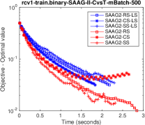
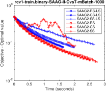
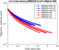
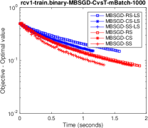
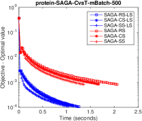
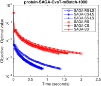
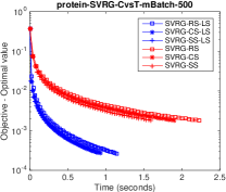
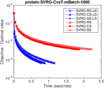
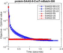
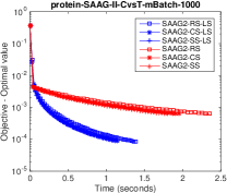
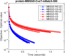
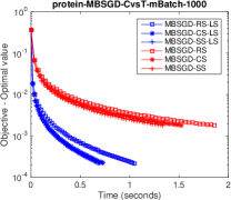
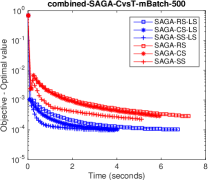
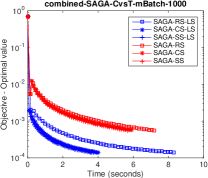
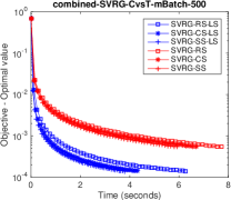
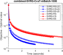
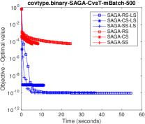
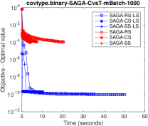
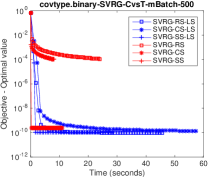
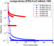
Experimental results plot the difference between objective function and optimum value against training time for three sampling techniques, namely, Random Sampling (RS), Cyclic/Sequential Sampling (CS) and Systematic Sampling (SS), which are represented by Figs.1–4. To save space, results for different samplings with constant step size and backtracking line search methods are plotted in same figure (red color for constant step size and blue for line search (LS)). As it is clear from figures, 20 different settings over one dataset compare CS, SS and RS, and prove that methods with CS and SS converges faster than with RS. In general, SS gives the best results as per the intuition but sometimes CS produces better results than SS since CS and SS are quite similar. The results with constant step size and backtracking line search methods show similar results. For larger datasets, like SUSY and HIGGS, SS and CS show clear advantage over RS, than for smaller dataset and thus prove the efficacy/suitability of CS and SS for large-scale learning problems. For some of the results, like, with HIGGS dataset and SAG method, learning algorithms with all the sampling techniques converge quickly to same value but careful examination reveals that CS and SS converges earlier than RS.

(a)

(b)

(c)

(d)

(e)

(f)

(g)

(h)

(i)

(j)

(k)

(l)

(m)

(n)

(o)

(p)

(q)

(r)

(s)

(t)

Figure 1: RS, CS and SS are compared using SAG, SAGA, SVRG, SAAG-II and MBSGD, each with two step determination techniques, namely, constant step and backtracking line search, over SUSY and rcv1 datasets with mini-batch of 500 and 1000 data points.

(a)

(b)

(c)

(d)

(e)

(f)

(g)

(h)

(i)

(j)

(k)

(l)

(m)

(n)

(o)

(p)

(q)

(r)

(s)

(t)

Figure 2: RS, CS and SS are compared using SAG, SAGA, SVRG, SAAG-II and MBSGD, each with two step determination techniques, namely, constant step and backtracking line search, over ijcnn1 and protein datasets with mini-batch of 500 and 1000 data points.

(a)

(b)

(c)

(d)

(e)

(f)

(g)

(h)

(i)

(j)

(k)

(l)

(m)

(n)

(o)

(p)

(q)

(r)

(s)

(t)

Figure 3: RS, CS and SS are compared using SAG, SAGA, SVRG, SAAG-II and MBSGD, each with two step determination techniques, namely, constant step and backtracking line search, over HIGGS and SensIT (combined) datasets with mini-batch of 500 and 1000 data points.

(a)

(b)

(c)

(d)

(e)

(f)

(g)

(h)

(i)

(j)

(k)

(l)

(m)

(n)

(o)

(p)

(q)

(r)

(s)

(t)

Figure 4: RS, CS and SS are compared using SAG, SAGA, SVRG, SAAG-II and MBSGD, each with two step determination techniques, namely, constant step and backtracking line search, over mnist and covtype datasets with mini-batch of 500 and 1000 data points.

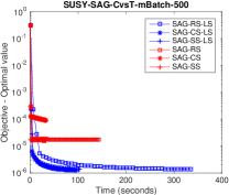
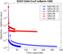
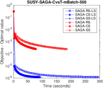
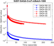
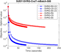
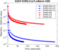
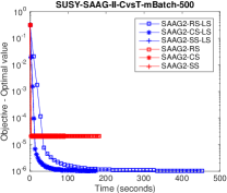
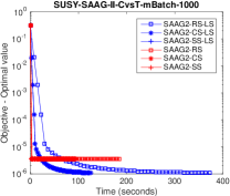
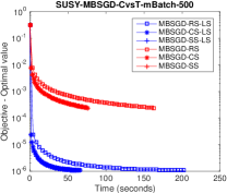
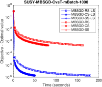
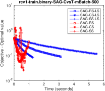
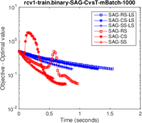
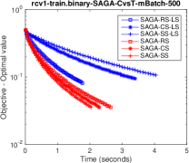
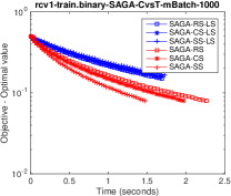
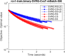
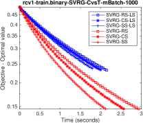
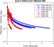
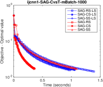
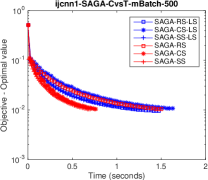
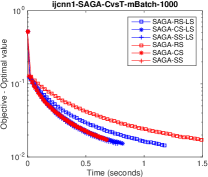
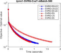
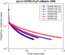
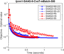
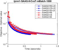
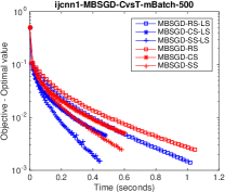
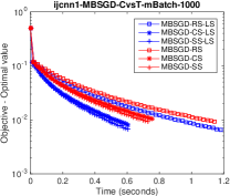
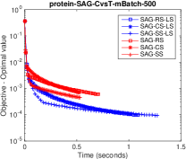
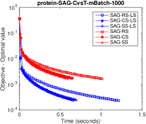
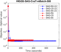
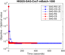
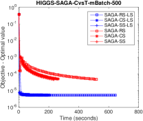
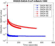
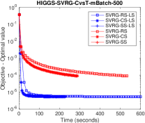
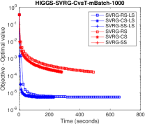
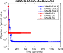
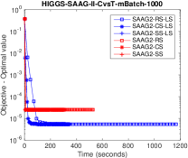
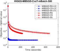
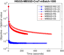
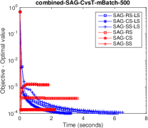
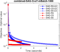
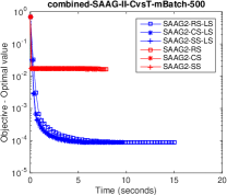
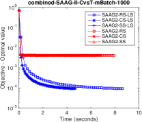
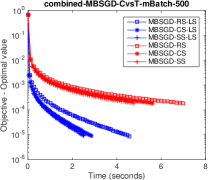
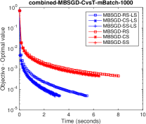
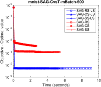
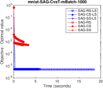
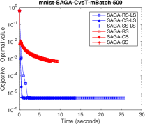
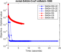
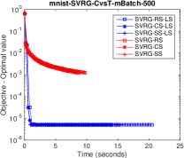
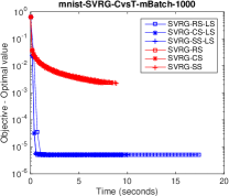
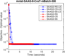
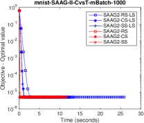
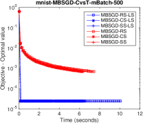
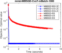
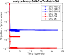
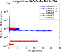
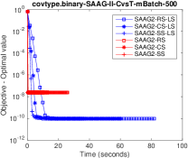
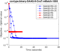
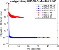
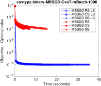
Experimental results can be presented using tables comparing the training time and objective function value, for given number of epochs (number of passes through dataset), for CS, SS and RS. Since it is easy to understand the graphs so experiments are documented using figures. Results for SUSY, HIGGS and covtype.binary are also represented using Tables 2, 3 and 4, which prove faster training for CS and SS than RS, while their values are same up to certain decimal places. As it is clear from the table, SAG method with mini-batch of size 200 and constant step size, the training time for Systematic Sampling (SS) and Cyclic Sampling (CS) are faster than for Random Sampling (RS) by a factor of more than three while the values of objective function are same up to four decimal places. The training times for SS and CS are very close as expected. For mini-batch of 1000 data points and constant step size, SAG method runs three and half times faster for SS and CS as compared with RS while the values of objective function are same up to six decimal places. With backtracking line search for determining the step size, SAG method runs more than two times faster with mini-batch of 200 and more than three and half times with mini-batch of size 1000, for SS and CS as compared with RS while the values of objective function are same up to eight decimal places. SAGA with constant step size runs more than two times faster with mini-batches of 200 and 1000 for CS and SS as compared with RS while the values of objective function are same up to five and four decimal places for mini-batches of 200 and 1000, respectively. With backtracking line search, SAGA performs even better for CS and SS and runs more than two times faster with mini-batch of 200 and more than three and half times with mini-batch of size 1000 as compared with RS while the values of objective function are same up to eight decimal places with mini-batch of size 200 and up to six decimal places with mini-batch of size 1000. Similar trend are followed for SAAG-II, SVRG and MBSGD methods where CS and SS are around two to more than three and half times faster and objective values are same up to six to nine decimal places as compared with RS with constant step and backtracking line search (LS).
Results with SUSY dataset are presented in Table 3. As it is clear from the table, it shows good results like HIGGS dataset. CS and SS techniques are faster than RS technique by around two to four times while the objective function values are same up to three to eight decimal places. Methods with constant step and with backtracking line search show similar trends for the results.
Results with covtype.binary dataset are presented in Table 4. As it is clear from the table, it gives good results. CS and SS techniques are faster than RS technique by around one and half to six times while the objective function values are same up to three to ten decimal places. Methods with constant step and with backtracking line search show similar trends but for line search, objective function values are close among each other.

Table 2: Comparison of Training Time (in seconds) and objective function values after 30 epochs using dataset HIGGS

Method	Sampling	Batch	Constant Step		Line Search
			Time	Objective	Time	Objective
SAG	RS	200	229.220102	0.3258410619	495.873963	0.3258353956
	CS		66.378361	0.3258375894	214.083371	0.3258353935
	SS		67.867812	0.3258410840	214.533017	0.3258353956
	RS	1000	234.129248	0.3258356616	535.821883	0.3258354793
	CS		63.957239	0.3258358353	126.807235	0.3258354785
	SS		65.908254	0.3258356562	148.786983	0.3258354792
SAGA	RS	200	302.318358	0.3258637650	432.787547	0.3258353922
	CS		147.235962	0.3258659974	182.545531	0.3258353924
	SS		148.402540	0.3258636638	177.698227	0.3258353937
	RS	1000	301.003253	0.3259746991	445.741781	0.3258354946
	CS		145.917197	0.3259814282	112.433248	0.3258355048
	SS		147.646753	0.3259748885	120.481113	0.3258354828
SAAG-II	RS	200	297.134694	0.3263398874	708.881659	0.3258353918
	CS		174.232600	0.3263398971	380.852014	0.3258353920
	SS		176.845275	0.3263398982	338.122579	0.3258353920
	RS	1000	299.840227	0.3258550019	687.638964	0.3258354037
	CS		171.384496	0.3258550023	209.564000	0.3258354039
	SS		172.268358	0.3258550036	213.877001	0.3258354041
SVRG	RS	200	297.620959	0.3258923266	406.229956	0.3258354055
	CS		172.405902	0.3258923398	213.151577	0.3258354059
	SS		172.612984	0.3258923141	185.538374	0.3258354064
	RS	1000	297.259155	0.3261069018	497.501496	0.3258357363
	CS		172.227776	0.3261069217	159.518159	0.3258357365
	SS		172.601618	0.3261068804	151.230547	0.3258357352
MBSGD	RS	200	267.252470	0.3258635308	312.865696	0.3258353862
	CS		144.769059	0.3258635315	121.004686	0.3258353865
	SS		140.241334	0.3258635313	122.396247	0.3258353867
	RS	1000	268.102817	0.3259704996	306.236327	0.3258354906
	CS		139.586141	0.3259704998	82.340378	0.3258354912
	SS		135.646766	0.3259704994	81.486252	0.3258354909

Table 3: Comparison of Training Time (in seconds) and objective function values after 30 epochs using dataset SUSY

Method	Sampling	Batch	Constant Step		Line Search
			Time	Objective	Time	Objective
SAG	RS	200	84.331058	0.3759925588	267.199348	0.3759914171
	CS		20.571099	0.3759958448	96.172599	0.3759912712
	SS		20.380268	0.3759925419	136.218536	0.3759914133
	RS	1000	86.462106	0.3761630312	261.746213	0.3759920053
	CS		19.652540	0.3764117775	45.862451	0.3759919137
	SS		23.803318	0.3761654289	56.056274	0.3759920025
SAGA	RS	200	119.419700	0.3761615578	244.424858	0.3759911729
	CS		49.054361	0.3761668056	88.012460	0.3759911528
	SS		50.032764	0.3761616154	125.125252	0.3759911723
	RS	1000	115.240795	0.3767228974	218.120526	0.3759920084
	CS		48.484855	0.3767380851	41.586102	0.3759920131
	SS		53.076179	0.3767231692	47.792283	0.3759919544
SAAG-II	RS	200	122.687745	0.3761359459	319.227862	0.3759910754
	CS		57.748874	0.3761359525	150.975243	0.3759910741
	SS		58.840208	0.3761359506	156.970161	0.3759910768
	RS	1000	114.239646	0.3759934574	336.178564	0.3759912580
	CS		58.377580	0.3759934575	88.889686	0.3759912583
	SS		67.017390	0.3759934576	88.760368	0.3759912574
SVRG	RS	200	128.216331	0.3763077569	215.183518	0.3759913085
	CS		57.819864	0.3763078069	88.178545	0.3759913110
	SS		60.425710	0.3763079011	98.404560	0.3759913135
	RS	1000	112.850682	0.3773260313	192.681710	0.3759936315
	CS		58.064456	0.3773259828	57.283939	0.3759936439
	SS		66.207054	0.3773261006	58.508361	0.3759936213
MBSGD	RS	200	101.673967	0.3761560102	174.388236	0.3759910145
	CS		47.587231	0.3761559893	58.634676	0.3759910107
	SS		48.042649	0.3761559954	63.347389	0.3759910169
	RS	1000	103.513668	0.3766979888	128.650218	0.3759918962
	CS		47.346182	0.3766979329	31.396945	0.3759918950
	SS		55.683464	0.3766979490	41.701046	0.3759918931

Table 4: Comparison of Training Time (in seconds) and objective function values after 30 epochs using dataset covtype.binary

Method	Sampling	Batch	Constant Step		Line Search
			Time	Objective	Time	Objective
SAG	RS	200	7.688000	0.0000000003	16.485357	0.0000009291
	CS		2.158810	0.0000000002	5.874758	0.0000024168
	SS		1.796637	0.0000000004	3.327142	0.0000005212
	RS	1000	7.624630	0.0000000015	20.674648	0.0000003902
	CS		2.110367	0.0000014178	3.436548	0.0000006984
	SS		1.608393	0.0000000003	4.217670	0.0000012383
SAGA	RS	200	9.512428	0.0000398812	33.541463	0.0000000001
	CS		4.200649	0.0000425219	36.688386	0.0000000001
	SS		2.909938	0.0000370651	23.002344	0.0000000001
	RS	1000	9.378465	0.0001809634	34.770427	0.0000000001
	CS		4.049684	0.0001901968	7.649198	0.0000000002
	SS		2.414478	0.0001763171	19.890575	0.0000000001
SAAG-II	RS	200	8.510917	0.0000001565	44.963308	0.0000000001
	CS		4.568239	0.0000001565	37.523382	0.0000000001
	SS		2.729112	0.0000001566	17.364469	0.0000000001
	RS	1000	13.558037	0.0000000063	56.251227	0.0000000001
	CS		6.355990	0.0000000063	37.831273	0.0000000001
	SS		4.325896	0.0000000063	19.511468	0.0000000001
SVRG	RS	200	9.370933	0.0000771729	32.835999	0.0000000001
	CS		5.234851	0.0000000005	39.737523	0.0000000001
	SS		3.645048	0.0000759334	21.836150	0.0000000001
	RS	1000	10.200179	0.0003404686	23.870644	0.0000000001
	CS		5.031777	0.0000009870	34.195127	0.0000000001
	SS		3.609489	0.0003181269	7.203759	0.0000000005
MBSGD	RS	200	8.314825	0.0000390866	27.593407	0.0000000001
	CS		4.142554	0.0000393200	17.189169	0.0000000001
	SS		3.050657	0.0000391765	11.707410	0.0000000001
	RS	1000	8.966491	0.0001756815	11.959532	0.0000000001
	CS		3.979792	0.0001747116	18.732325	0.0000000001
	SS		2.456082	0.0001707026	9.960456	0.0000000001

5 Conclusion

In this paper, novel systematic sampling and cyclic sampling techniques have been proposed, for solving large-scale learning problems, for improving the training time by reducing the data access time. Methods have similar convergence in expectation for systematic and cyclic sampling, as for widely used random sampling, but with cyclic and systematic sampling the training is up to six times faster than widely used random sampling technique, at the expense of fractionally small difference in the minimized objective function value, for a given number of epochs. Thus, systematic sampling technique is suitable for solving large-scale problem with low accuracy solution. Random shuffling of data can be used before the data is fed to the learning algorithms with systematic and cyclic sampling to improve their results for the cases where similar data points are grouped together. These sampling techniques can be extended to parallel and distributed learning algorithms.

References

- Byrd et al (2016) Byrd RH, Hansen SL, Nocedal J, Singer Y (2016) A stochastic quasi-newton method for large-scale optimization. SIAM Journal on Optimization 26(2):1008–1031
- Chang et al (2008) Chang KW, Hsieh CJ, Lin CJ (2008) Coordinate descent method for large-scale l2-loss linear support vector machines. J Mach Learn Res 9:1369–1398
- Chauhan et al (2017) Chauhan VK, Dahiya K, Sharma A (2017) Mini-batch block-coordinate based stochastic average adjusted gradient methods to solve big data problems. In: Proceedings of the Ninth Asian Conference on Machine Learning, PMLR, vol 77, pp 49–64, URL http://proceedings.mlr.press/v77/chauhan17a.html
- Chauhan et al (2018a) Chauhan VK, Dahiya K, Sharma A (2018a) Faster algorithms for large-scale machine learning using simple sampling techniques. arXiv URL https://arxiv.org/abs/1801.05931v2
- Chauhan et al (2018b) Chauhan VK, Dahiya K, Sharma A (2018b) Problem formulations and solvers in linear svm: a review. Artificial Intelligence Review DOI 10.1007/s10462-018-9614-6, URL https://doi.org/10.1007/s10462-018-9614-6
- Chauhan et al (2018c) Chauhan VK, Sharma A, Dahiya K (2018c) Faster learning by reduction of data access time. Applied Intelligence DOI 10.1007/s10489-018-1235-x, URL https://doi.org/10.1007/s10489-018-1235-x
- Chauhan et al (2018d) Chauhan VK, Sharma A, Dahiya K (2018d) SAAGs: Biased Stochastic Variance Reduction Methods. arXiv URL http://arxiv.org/abs/1807.08934, 1807.08934
- Cotter et al (2011) Cotter A, Shamir O, Srebro N, Sridharan K (2011) Better Mini-Batch Algorithms via Accelerated Gradient Methods. Nips pp 1–9, URL http://arxiv.org/abs/1106.4574, 1106.4574
- Csiba and Richt (2016) Csiba D, Richt P (2016) Importance Sampling for Minibatches pp 1–19, arXiv:1602.02283v1
- Csiba and Richtárik (2016) Csiba D, Richtárik P (2016) Coordinate Descent Face-Off: Primal or Dual? pp 1–17, 1605.08982
- Defazio et al (2014) Defazio A, Bach F, Lacoste-Julien S (2014) Saga: A fast incremental gradient method with support for non-strongly convex composite objectives. In: Proceedings of the 27th International Conference on Neural Information Processing Systems, MIT Press, Cambridge, MA, USA, NIPS’14, pp 1646–1654
- Gopal (2016) Gopal S (2016) Adaptive Sampling for SGD by Exploiting Side Information. Icml
- Johnson and Zhang (2013) Johnson R, Zhang T (2013) Accelerating stochastic gradient descent using predictive variance reduction. In: Burges CJC, Bottou L, Welling M, Ghahramani Z, Weinberger KQ (eds) Advances in Neural Information Processing Systems 26, Curran Associates, Inc., pp 315–323
- Konečný and Richtárik (2013) Konečný J, Richtárik P (2013) Semi-Stochastic Gradient Descent Methods 1:19, URL http://arxiv.org/abs/1312.1666, 1312.1666
- Li et al (2014) Li M, Zhang T, Chen Y, Smola AJ (2014) Efficient mini-batch training for stochastic optimization. In: Proceedings of the 20th ACM SIGKDD International Conference on Knowledge Discovery and Data Mining, ACM, New York, NY, USA, KDD ’14, pp 661–670
- Madow (1949) Madow WG (1949) On the theory of systematic sampling, ii. The Annals of Mathematical Statistics 20:333–354, URL http://www.jstor.org/stable/2236532
- Madow and Madow (1944) Madow WG, Madow LH (1944) On the theory of systematic sampling, i. The Annals of Mathematical Statistics 15:1–24, URL http://www.jstor.org/stable/2236209
- Needell et al (2014) Needell D, Ward R, Srebro N (2014) Stochastic gradient descent, weighted sampling, and the randomized kaczmarz algorithm. In: Ghahramani Z, Welling M, Cortes C, Lawrence ND, Weinberger KQ (eds) Advances in Neural Information Processing Systems 27, Curran Associates, Inc., pp 1017–1025
- Nemirovski et al (2009) Nemirovski A, Juditsky A, Lan G, Shapiro A (2009) Robust stochastic approximation approach to stochastic programming. SIAM Journal on Optimization 19(4):1574–1609
- Qu and Richt (2015) Qu Z, Richt P (2015) Randomized Dual Coordinate Ascent with Arbitrary Sampling. Neural Information Processing Systems (1):1–34, arXiv:1411.5873v1
- Reddi (2016) Reddi SJ (2016) New Optimization Methods for Modern Machine Learning. PhD thesis
- Schmidt et al (2016) Schmidt M, Le Roux N, Bach F (2016) Minimizing finite sums with the stochastic average gradient. Math Program pp 1–30
- Shalev-Shwartz et al (2011) Shalev-Shwartz S, Singer Y, Srebro N, Cotter A (2011) Pegasos: primal estimated sub-gradient solver for svm. Math Program 127(1):3–30
- Takáč et al (2013) Takáč M, Bijral A, Richtárik P, Srebro N (2013) Mini-batch primal and dual methods for svms. In: In 30th International Conference on Machine Learning, Springer, pp 537–552
- Wang et al (2017) Wang X, Wang S, Zhang H (2017) Inexact proximal stochastic gradient method for convex composite optimization. Computational Optimization and Applications DOI 10.1007/s10589-017-9932-7, URL https://doi.org/10.1007/s10589-017-9932-7
- Wright (2015) Wright SJ (2015) Coordinate descent algorithms. Math Program 151(1):3–34
- Xu and Yin (2015) Xu Y, Yin W (2015) Block stochastic gradient iteration for convex and nonconvex optimization. SIAM Journal on Optimization 25(3):1686–1716
- Yu et al (2010) Yu HF, Hsieh CJ, Chang KW, Lin CJ (2010) Large linear classification when data cannot fit in memory. In: Proceedings of the 16th ACM SIGKDD International Conference on Knowledge Discovery and Data Mining, ACM, New York, NY, USA, KDD ’10, pp 833–842
- Zhang and Gu (2016) Zhang A, Gu Q (2016) Accelerated stochastic block coordinate descent with optimal sampling. In: Proceedings of the 22Nd ACM SIGKDD International Conference on Knowledge Discovery and Data Mining, ACM, New York, NY, USA, KDD ’16, pp 2035–2044
- Zhang (2004) Zhang T (2004) Solving large scale linear prediction problems using stochastic gradient descent algorithms. In: Proceedings of the Twenty-first International Conference on Machine Learning, ACM, New York, NY, USA, ICML ’04, pp 116–
- Zhao and Zhang (2014) Zhao P, Zhang T (2014) Accelerating Minibatch Stochastic Gradient Descent using Stratified Sampling. arXiv Prepr arXiv14053080 pp 1–13, URL http://arxiv.org/abs/1405.3080
- Zhao and Zhang (2015) Zhao P, Zhang T (2015) Stochastic Optimization with Importance Sampling for Regularized Loss Minimization. ICML 37
- Zhou et al (2017) Zhou L, Pan S, Wang J, Vasilakos AV (2017) Machine learning on big data: Opportunities and challenges. Neurocomputing 237:350 – 361, DOI https://doi.org/10.1016/j.neucom.2017.01.026, URL https://www.sciencedirect.com/science/article/pii/S0925231217300577