Coordinate Descent Face-Off: Primal or Dual?
Abstract
Randomized coordinate descent (RCD) methods are state-of-the-art algorithms for training linear predictors via minimizing regularized empirical risk. When the number of examples () is much larger than the number of features (), a common strategy is to apply RCD to the dual problem. On the other hand, when the number of features is much larger than the number of examples, it makes sense to apply RCD directly to the primal problem. In this paper we provide the first joint study of these two approaches when applied to L2-regularized ERM. First, we show through a rigorous analysis that for dense data, the above intuition is precisely correct. However, we find that for sparse and structured data, primal RCD can significantly outperform dual RCD even if , and vice versa, dual RCD can be much faster than primal RCD even if . Moreover, we show that, surprisingly, a single sampling strategy minimizes both the (bound on the) number of iterations and the overall expected complexity of RCD. Note that the latter complexity measure also takes into account the average cost of the iterations, which depends on the structure and sparsity of the data, and on the sampling strategy employed. We confirm our theoretical predictions using extensive experiments with both synthetic and real data sets.
1 Introduction
In the last 5 years or so, randomized coordinate descent (RCD) methods [22, 12, 18, 19] have become immensely popular in a variety of machine learning tasks, with supervised learning being a prime example. The main reasons behind the rise of RCD-type methods is that they can be easily implemented, have intuitive appeal, and enjoy superior theoretical and practical behaviour when compared to classical methods such as SGD [20], especially in high dimensions, and in situations when solutions of medium to high accuracy are needed. One of the most important success stories of RCD is in the domain of training linear predictors via regularized empirical risk minimization (ERM).
The highly popular SDCA algorithm [24] arises as the application of RCD [18] to the dual problem associated with the (primal) ERM problem111Indeed, the analysis of SDCA in [24] proceeds by applying the complexity result from [18] to the dual problem, and then arguing that the same rate applies to the primal suboptimality as well.. In practice, SDCA is most effective in situations where the number of examples () exceeds the number of features (). Since the dual of ERM is an dimensional problem, it makes intuitive sense to apply RCD to the dual. Indeed, RCD can be seen as a randomized decomposition strategy, reducing the dimensional problem to a sequence of (randomly generated) one-dimensional problems.
However, if the number of features exceeds the number of examples, and especially when the difference is very large, RCD methods [19] have been found very attractive for solving the primal problem (i.e., the ERM problem) directly. For instance, distributed variants of RCD, such as Hydra [17] and its accelerated cousin Hydra2 [3] have been successfully applied to solving problems with billions of features.
Recently, a variety of novel primal methods for ERM have been designed, including SAG [21], SVRG [5], S2GD [8], proxSVRG [25], mS2GD [6], SAGA [2], MISO [10] and S2CD [7]. As SDCA, all these methods improve dramatically on SGD [20] as a benchmark, which they achieve by employing one of a number of variance-reduction strategies. However, these methods have essentially identical identical theoretical behavior to SDCA, including the property that these methods thrive in the data-laden domain (i.e., ). In this sense, in our comparison of primal vs dual RCD, these methods should be viewed as “dual methods”.
1.1 Contributions
In this paper we provide the first joint study of these two approaches—applying RCD to the primal vs dual problems—and we do so in the context of L2-regularized ERM. First, we show through a rigorous theoretical analysis that for dense data, the intuition that the primal approach is better than the dual approach when , and vice versa, is precisely correct. However, we show that for sparse data, this does not need to be the case: primal RCD can significantly outperform dual RCD even if , and vice versa, dual RCD can be much faster than primal RCD even if . In particular, we identify that the face-off between primal and dual RCD boils down to the comparison of as single quantity associated with the data matrix and its transpose. Moreover, we show that, surprisingly, a single sampling strategy minimizes both the (bound on the) number of iterations and the overall expected complexity of RCD. Note that the latter complexity measure takes into account also the average cost of the iterations, which depends on the structure and sparsity of the data, and on the sampling strategy employed. We confirm our theoretical findings using extensive experiments with both synthetic and real data sets.
2 Primal and Dual Formulations of ERM
Let be a data matrix, with referring to the number of examples and to the number of features. With each example we associate a loss function , and pick a regularization constant . The key problem of this paper is the L2-regularized ERM problem
| (1) |
where denotes the standard Euclidean inner product and . We refer to (1) as the primal problem. We assume throughout that the functions are convex and -smooth:
| (2) |
The dual problem of (1) is
| (3) |
where is the convex conjugate of , defined by It is well known that [24, 15] that for every pair and . Moreover, the primal and dual optimal solutions, and , respectively, are unique, and satisfy the relations and for all , which also uniquely characterize them.
3 Primal and Dual RCD
In its general “arbitrary sampling” form [16], RCD applied to the primal problem (1) has the form
| (4) |
where are parameters of the method and is the th partial derivative of at . This update is performed for a random subset of the coordinates chosen in an i.i.d. fashion according to some sampling . The parameters are computed ahead of the iterative process and need to be selected carefully in order for the method to work [16, 14]. Specifically, one can set , where is chosen so as to satisfy the ESO (expected separable overapproximation) inequality
| (5) |
where is the matrix with entries , and denotes the Hadamard (element-wise) product of matrices. The method is formally described as Algorithm 1.
When applying RCD to the dual problem 3, we can’t proceed as above since the functions are not necessarily smooth, and hence we can’t compute the partial derivatives of the dual objective. The standard approach here is to use a proximal variant of RCD [19]. In particular, Algorithm 2 has been analyzed in [15]. Like Algorithm 1, Algorithm 2 is also capable to work with an arbitrary sampling, which in this case is a random subset of . The ESO parameters must in this case satisfy the ESO inequality
| (6) |
where is an matrix with entries and .
4 Iteration Complexity and Total Arithmetic Complexity
In this section we give expressions for the total expected arithmetic complexity of the two algorithms.
4.1 Number of iterations
Iteration complexity of Algorithms 1 and 2 is described in the following theorem. We include a proof sketch in the appendix.
Theorem 1.
(Complexity: Primal vs Dual RCD)
Let be convex and -smooth.
(i) If is proper (i.e., for all ), and satisfies (5), then iterates of primal RCD satisfy
| (8) |
where is a constant depending on and .
(ii) If is proper (i.e., for all ), and satisfies (6), then iterates of dual RCD satisfy
| (9) |
where is a constant depending on and .
For the dual method a stronger guarantee can be established (see [15]): as soon as , we have . Clearly, this stronger result implies the claim in part ii) of the above theorem.
4.2 Average cost of a single iteration
Let be the number of nonzeros in a matrix/vector. It is easy to observe that the average cost of a single iteration of Algorithm 1 is
| (10) |
and for Algorithm 2 it is
| (11) |
We remark that the constant hidden in may be larger for Algorithm 1 than for Algorithm 2. The reason for this is that for Algorithm 1 we compute the one-dimensional derivative for every nonzero term in the sum, while for Algorithm 2 we do this only once. Depending on the loss , this may lead to slower iterations. For example, if isthe logistic loss, experimentation shows that the constant is around 50. On the other hand, if is the squared loss, the constant is 1.
4.3 Total complexity
5 Choosing a Sampling that Minimizes the Total Complexity
In this section we identify the optimal sampling in terms of the total complexity. This is different from previous results on importance sampling, which neglect to take into account the cost of the iterations [16, 15, 27, 11]. For simplicity, we shall only consider serial samplings, i.e., samplings which only pick a single coordinate at a time. The situation is much more complicated with non-serial samplings where first importance sampling results have only been derived recently [1].
5.1 Uniform Sampling
The simplest serial sampling is the uniform sampling: it selects every coordinate with the same probability, i.e. and . In view of (12), (13) and (7), we get
and
We can now clearly see that whether or depends does not simply depend on vs , but instead depends on the relative value of the quantities and . Having said that, we shall not study these quantities in this paper. The reason for this is that for the cake of brevity, we shall instead focus on comparing the primal and dual RCD methods for optimal sampling which minimizes the total complexity, in which case we will obtain different quantities.
5.2 Importance Sampling
By importance sampling we mean the serial sampling (resp. ) which minimizes the bounds in 8 (resp. in (9)). It can easily be seen (see also [16], [15], [27]), that importance sampling probabilities are given by
| (14) |
On the other hand, one can observe that the average iteration cost of importance sampling may be larger than the average iteration cost of uniform serial sampling. Therefore, it is a natural question to ask, whether it is necessarily better. In view of (12), (13) and (14), the total complexities for importance sampling are
| (15) |
Since a weighted average is smaller than the maximum, the total complexity of both methods with importance sampling is always better than with uniform sampling. However, this does not mean that importance sampling is the sampling that minimizes total complexity.
5.3 Optimal Sampling
The next theorem states that, in fact, importance sampling does minimize the total complexity.
Theorem 2.
The optimal serial sampling (i.e., the serial sampling minimizing the total expected complexity (resp, )) is the importance sampling (14).
6 The Face-Off
In this section we investigate the two quantities in (15), and , measuring the total complexity of the two methods as functions of the data . Clearly, it is enough to focus on the quantities
| (16) |
We shall ask questions such as: when is larger/smaller than , and by how much. In this regard, it is useful to note that . Our first result gives tight lower and upper bounds on their ratio.
Theorem 3.
For any with no zero rows or columns, we have the bounds and . It follows that Moreover, all these bounds are tight.
Since (resp. ) can dominate the expression (12) (resp. (13)) for total complexity, it follows that, depending on the data matrix , the primal method can be up to times faster than the dual method, and up to times slower than the dual method.
6.1 Random Data and Dense Data
Assume now that the entries of are chosen in an i.i.d. manner from some distribution with mean and variance . While this is not a realistic scenario, it will help us build intuition about what we can expect the quantities and to look like. A simple calculation reveals that , and . Hence,
precisely when , which means that the primal method is better when and the dual method is better when .
If is a dense deterministic matrix ( for all ), then and , and we reach the same conclusion as for random data: everything boils down to vs .
6.2 Binary Data
In this part we identify a class of data matrices for which one can have even if . This class is by no means exhaustive, and serves as an example which we use to illustrate the phenomenon.
Let denote the set of matrices with (signed) binary elements, i.e., with for all . For , the expressions in (16) can be also written in the form and . By we denote the set of all matrices in with nonzero columns and rows.
For positive integers we write (i.e., rounded down to the closest multiple of ). Further, we write
where
and
The following is a refinement of Theorem 3 for binary matrices of fixed cardinality .
Theorem 4.
For all with we have the bounds . Moreover, these bounds are tight.
The above theorem follows from Lemma 9, which we formulate and prove in the Appendix. This lemma establishes formulas for the minimum and maximum of and , subject to the constraint , in terms of the functions and . Further, as we show in Lemma 10 in the Appendix, if and , then . Likewise, if and , then . Combined with Theorem 4, this has an interesting consequence, spelled out in the next theorem and its corollary.
Theorem 5.
Let . If and , then . By symmetry, if and , then .
This result says that for binary data, and , the primal method is better than the dual method even for non-dense data, as long as the the data is “dense enough”. Observe that as long as , all matrices satisfy . This leads to the following corollary.
Corollary 6.
If , then for all we have . By symmetry, if , then for all we have .
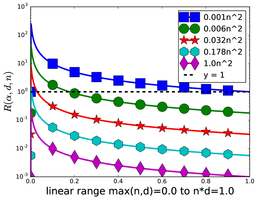
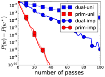
In words, the corollary states that for binary data where the number of features () is large enough in comparison with the number of examples (), the primal method will be always better. On the other hand, if is large enough, the dual method will be always better. This behavior can be observed in Figure 1. For large enough , all the values are below 1.
7 Experiments
We conducted experiments on both real and synthetic data. The problem we were interested in is a standard logistic regression with an L2-regularizer, i.e.,
In all our experiments we used and we normalized all the entries of by the average column norm. Note that for logistic loss there is no closed form solution for in Algorithm 2. Therefore we use a variant of Algorithm 2 where with the step size defined as . This variant has the same convergence rate guarantees as Algorithm 2 and does not require exact minimization. Details can be found in [15].
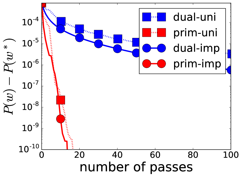
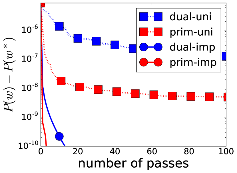
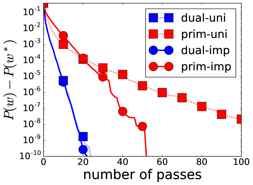
We plot the training error against the number of passes through the data. The number of passes is calculated according to the number of visited nonzero entries in the matrix . One pass means that we look at nonzero entries of , but not necessarily all of them. We look at the problems from the perspective of the primal approach. The same could be done symmetrically for the dual approach.
7.1 General Data
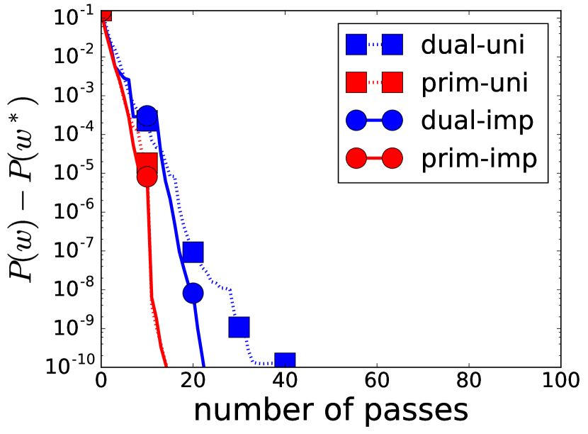
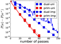
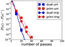
We look at the matrices which give worst-case bounds for general matrices (Theorem 3) and their empirical properties for different choices of and . The corresponding figures are Figure 2(a) and 2(b). For a square dataset, we can observe a large speed-up. For large we can observe, that the theory holds and the primal method is still faster, but because of numerical issues (we need very small and very large numbers in matrix) and the fact that the optimal value is very close to an "initial guess" of the algorithm, the difference in speed is more difficult to observe.
7.2 Synthetic Binary Data
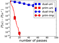
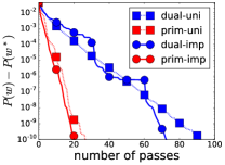
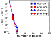
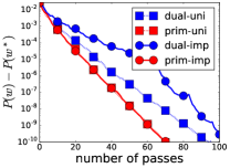
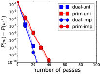
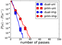
We looked at matrices with all entries in for some . We fixed the number of features to be and we varied the number of examples and the sparsity level . For each triplet we produced the worst-case matrix for dual RCD according to the developed theory. The results are in Figure 3.
| nnz | nnz | nnz | |
|
|
|
|
|
|
|
|
|
|
|
|
|
|
|
7.3 Real Data
We used two real datasets to showcase our theory: news and leukemia222both datasets are available from https://www.csie.ntu.edu.tw/ cjlin/libsvmtools/datasets/. The news dataset in Figure 2(c) is a nice example of our theory in practice. As shown in Table 1 we have , but the dual method is empirically faster than the primal one. The reason is simple: the news dataset uses a bag of words representation of news articles. If we look at the distribution of features (words), there are many words which appear just very rarely and there are words commonly used in many articles. The features have therefore a very skewed distribution of their nonzero entries. On the other hand, the examples have quite uniform distribution, as the number of distinct words in an article acts nicely. This distribution of nonzero entries highly favors the dual approach, as shown in the theory. The leukemia dataset in Figure 2(d) is a fully dense dataset and . Therefore, as our theoretical analysis shows, the primal approach should be better. The ratio between the runtimes is not very large, as the constant is of similar order as the additional term in the computation of the true runtime. The empirical speedup in Figures 2(c) and Figures 2(d) matches the theoretical predictions from Table 1.
| dataset | density | ||||||
|---|---|---|---|---|---|---|---|
| news | 1,355,191 | 19,996 | 0.03% | 9,097,916 | 2.0 | ||
| leukemia | 7,129 | 38 | 100.00% | 270,902 | 0.5 |
8 Conclusions and Extensions
We have shown that the question whether RCD should be applied to the primal or the dual problem depends on the structure of the training dataset. For dense data, this simply boils down to whether we have more data or parameters, which is intuitively appealing. We have shown, both theoretically, and through experiments with synthetic and real datasets, that contrary to what seems to be a popular belief, primal RCD can outperform dual RCD even if .
References
- [1] D. Csiba and P. Richtárik. Importance sampling for minibatches. arXiv:1602.02283, 2016.
- [2] A. Defazio, F. Bach, and S. Lacoste-Julien. SAGA: a fast incremental gradient method with support for non-strongly convex composite objectives. In NIPS 27, pages 1646–1654, 2014.
- [3] O. Fercoq, Z. Qu, P. Richtárik, and M. Takáč. Fast distributed coordinate descent for minimizing non-strongly convex losses. IEEE Int. Workshop on Machine Learning for Signal Processing, 2014.
- [4] O. Fercoq and P. Richtárik. Accelerated, parallel, and proximal coordinate descent. SIAM Journal on Optimization, 25(4):1997–2023, 2015.
- [5] R. Johnson and T. Zhang. Accelerating stochastic gradient descent using predictive variance reduction. In NIPS 26, 2013.
- [6] J. Konečný, J. Lu, P. Richtárik, and M. Takáč. mS2GD: Mini-batch semi-stochastic gradient descent in the proximal setting. IEEE J. of Selected Topics in Sig. Proc., 10(2):242–255, 2016.
- [7] J. Konečný, Z. Qu, and P. Richtárik. Semi-stochastic coordinate descent. arXiv:1412.6293, 2014.
- [8] J. Konečný and P. Richtárik. S2GD: Semi-stochastic gradient descent methods. arXiv:1312.1666, 2013.
- [9] Q. Lin, Z. Lu, and L. Xiao. An accelerated proximal coordinate gradient method. In NIPS 27, pages 3059–3067, 2014.
- [10] J. Mairal. Incremental majorization-minimization optimization with application to large-scale machine learning. SIAM Journal on Optimization, 25(2):829–855, 2015.
- [11] D. Needell, R. Ward, and N. Srebro. Stochastic gradient descent, weighted sampling, and the randomized kaczmarz algorithm. In NIPS 27, pages 1017–1025, 2014.
- [12] Yurii Nesterov. Efficiency of coordinate descent methods on huge-scale optimization problems. SIAM Journal on Optimization, 22(2):341–362, 2012.
- [13] Z. Qu and P. Richtárik. Coordinate descent with arbitrary sampling I: Algorithms and complexity. Optimization Methods and Software, 2016.
- [14] Z. Qu and P. Richtárik. Coordinate descent with arbitrary sampling II: Expected separable overapproximation. Optimization Methods and Software, 2016.
- [15] Z. Qu, P. Richtárik, and T. Zhang. Quartz: Randomized dual coordinate ascent with arbitrary sampling. In NIPS 28, pages 865–873. 2015.
- [16] P. Richtárik and M. Takáč. On optimal probabilities in stochastic coordinate descent methods. Optimization Letters, pages 1–11, 2015.
- [17] P. Richtárik and M. Takáč. Distributed coordinate descent method for learning with big data. JMLR, pages 1–25, 2016.
- [18] P. Richtárik and M. Takáč. Iteration complexity of randomized block-coordinate descent methods for minimizing a composite function. Mathematical Programming, 144(2):1–38, 2014.
- [19] P. Richtárik and M. Takáč. Parallel coordinate descent methods for big data optimization. Mathematical Programming, 156(1):433–484, 2015.
- [20] H. Robbins and S. Monro. A stochastic approximation method. Ann. Math. Statist., 22(3):400–407, 1951.
- [21] M. Schmidt, N. Le Roux, and F. Bach. Minimizing finite sums with the stochastic average gradient. arXiv:1309.2388, 2013.
- [22] S. Shalev-Shwartz and A. Tewari. Stochastic methods for -regularized loss minimization. JMLR, 12:1865–1892, 2011.
- [23] S. Shalev-Shwartz and T. Zhang. Accelerated mini-batch stochastic dual coordinate ascent. In NIPS 26, pages 378–385. 2013.
- [24] S. Shalev-Shwartz and T. Zhang. Stochastic dual coordinate ascent methods for regularized loss. JMLR, 14(1):567–599, 2013.
- [25] L. Xiao and T. Zhang. A proximal stochastic gradient method with progressive variance reduction. SIAM Journal on Optimization, 24(4):2057–2075, 2014.
- [26] Y. Zhang and L. Xiao. Stochastic primal-dual coordinate method for regularized empirical risk minimization. ICML, 2015.
- [27] P. Zhao and T. Zhang. Stochastic optimization with importance sampling. ICML, 2015.
APPENDIX
Proof of Theorem 1
We say that , if
For three vectors we define and Also, let for and , we write , where is the -th coordinate vector (i.e., standard basis vector) in .
We will need the following two lemmas.
Lemma 7.
The primal objective satisfies , where .
Proof.
∎
Lemma 8.
If and is such that , then
Proof.
See [14], Section 3. ∎
We can now proceed to the proof of Theorem 1.
First, note that
with defined as in (5). We now separately establish the two complexity results; (i) for primal RCD and (ii) for dual RCD.
(i) The proof is a consequence of the proof of the main theorem of [16]. Assumption 1 from [16] holds with (Lemma 7 & Lemma 8) and Assumption 2 from [16] holds with standard Euclidean norm and . We follow the proof all the way to the bound
which holds for defined by
by direct substitution of the quantities. The result follows by standard arguments. Note that
(ii) The proof is a direct consequence of the proof of the main theorem of [15], using the fact that , as the weak duality holds. Note that
Proof of Theorem 2
The proofs for Algorithm 1 and Algorithm 2 are analogous, and hence we will establish the result for Algorithm 1 only. For brevity, denote . We aim to solve the optimization problem:
| (17) |
First observe, that the problem is homogeneous in , i.e., if is optimal, also will be optimal for , as the solution will be the same. Using this argument, we can remove the constraint . Also, we can remove the multiplicative factor from the denominator as it does not change the . Hence we get the simpler problem
| (18) |
Now choose optimal and assume that there exist such that . By a small decrease in , we will still have , and hence the term stays unchanged. However, the term decreased. This means that the optimal sampling must satisfy for all . However, this is precisely the importance sampling.
Proof of Theorem 3
By assumption, all rows and columns of are nonzero. Therefore, and , and the bounds on and follow by applying this to (16). The bounds for the ratio follow immediately by combining the previous bounds. It remains to establish tightness. For , let be the matrix defined as follows:
Notice that does not have any zero rows nor columns as long as are nonzero. Since and , one readily sees that
Proof of Theorem 4
We first need a lemma.
Lemma 9.
Let be an integer satisfying and let and be the functions defined in Section 6.2. We have the following identities:
| (19) | |||||
| (20) | |||||
| (21) | |||||
| (22) |
Proof.
Let be an arbitrary matrix and let , where . Let . Observe that .
-
(i)
We shall first establish (19). Assume that the exist two columns of , such that , i.e., their difference in the number of nonzeros is at least 2. Because , there has to exist a row which has a nonzero entry in the -th column and a zero entry in the -th column. Let be the matrix obtained from by switching these two entries. Note that . However, we have
It follows that while there exist two such columns, the minimum is not achieved. So, we only need to consider matrices for which there exists integer such that or for every . Let .
We can now without loss of generality assume that . Indeed, we can do this is because the choices and lead to the same matrices, and hence by focusing on we have not removed any matrices from consideration. With simple calculations we get
Note that is a multiple of . It follows that and . Up to the ordering of the columns (which does not affect ) we have just one candidate , therefore it has to be the minimizer of . Finally, we can easily calculate the minimum as
- (ii)
-
(iii)
We now establish claim (21). Assume that there exist a pair of columns such that . Let be the matrix obtained from by zeroing out an entry in the -th column and putting a nonzero inside the -th column. Then
It follows that while there exist such a pair of columns, the maximum is not achieved. This condition leaves us with matrices where at most one column has not equal to 1 or .
Formally, let . Then we have columns with nonzero and 1 column with nonzeros, where . This is correct, as is the same as and being one more. We can compute and from the equation
as the only solution to the division with remainder of by , with the difference that instead of the standard . We get
The maximum can now be easily computed as follows:
- (iv)
∎
We can now proceed to the proof of the theorem.
The quantity is the ratio between the maximal value of and the minimal value of , we have to show that there exists a matrix such that this is achieved. Assume we have a matrix which has the maximal . In the proof of Lemma 9 we showed, that by switching entries in we can get the minimal value of without changing . Therefore we can achieve maximal and minimal at the same time. Analogically for every other case.
Proof of Theorem 5
As shown in the main text, the theorem follows from the following lemma. Hence, we only need to prove the lemma.
Lemma 10.
If and , then . If and , then .
Proof.
We focus on the first part, the second follows in an analogous way. Using the two assumptions, we have . By adding to the right hand side and after reshuffling, we obtain the inequality
For positive scalars , we have the trivial estimates . We use them to bound four expressions:
Using these bounds one-by-one we get the result
∎