Asymptotically (A)dS dilaton black holes with nonlinear electrodynamics

Abstract

It is well-known that with an appropriate combination of three Liouville-type dilaton potentials, one can construct charged dilaton black holes in an (anti)-de Sitter [(A)dS] spaces in the presence of linear Maxwell field. However, asymptotically (A)dS dilaton black holes coupled to nonlinear gauge field have not been found. In this paper, we construct, for the first time, three new classes of dilaton black hole solutions in the presence of three types of nonlinear electrodynamics, namely Born-Infeld, Logarithmic and Exponential nonlinear electrodynamics. All these solutions are asymptotically (A)dS and in the linear regime reduce to the Einstein-Maxwell-dilaton black holes in AdS spaces. We investigate physical properties and the causal structure, as well as asymptotic behavior of the obtained solutions, and show that depending on the values of the metric parameters, the singularity can be covered by various horizons. Interestingly enough, we find that the coupling of dilaton field and nonlinear gauge field in the background of (A)dS spaces leads to a strange behaviour for the electric field. We observe that the electric field is zero at singularity and increases smoothly until reaches a maximum value, then it decreases smoothly until goes to zero as $r\rightarrow\infty$. The maximum value of the electric field increases with increasing the nonlinear parameter $\beta$ or decreasing the dilaton coupling $\alpha$ and is shifted to the singularity in the absence of either dilaton field ($\alpha=0$) or nonlinear gauge field ($\beta\rightarrow\infty$).

PACS numbers: 04.70.Bw, 04.20.Ha, 04.20.Jb

I Introduction

The investigations on the black holes solutions in the background of AdS spacetimes have got renewed attentions in the two past decades. This is mostly due to the Maldacena’s conjecture which corresponds a gravity theory in an AdS space with a conformal field theory (CFT) living on the boundary of this space, known as AdS/CFT correspondence maldacena . Based on this duality, thermodynamics of black holes in $n$-dimensional AdS space can be identified with that of a certain dual CFT in the high temperature limit on the $(n-1)$-dimensional boundary of this spacetime. In fact, the AdS/CFT correspondence provides an ideal tool to study strongly coupled field theories. For example, many authors have investigated condensed matter systems such as superconductors via this correspondence SC . Moreover, it was shown that a relevance exists between thermodynamic variables and the stress-energy tensor of large, rotating black holes and fluids on its conformal boundary Bhattacharyya . This fact further motivates theoretical physicists to study black holes in the background of (A)dS spaces.

The motivation of perusing dilaton field comes from the fact that this field appears in the low energy limit of string theory where the Einstein action is supplemented with other fields like axion, gauge fields and scalar dilaton field. The dilaton field changes the causal structure of the black hole and leads to the curvature singularities at finite radii. In the absence of dilaton potential, exact solutions of charged dilaton black holes have been constructed by many authors CDB1 ; CDB2 . These black holes are all asymptotically flat. It was shown that the presence of the dilaton potential, which can be regarded as the generalization of the cosmological constant, can change the asymptotic behavior of the solutions to be neither flat nor (A)dS. Indeed, it was shown that, no dilaton (A)dS black hole solution exists with the presence of only one Liouville-type dilaton potential MW . In the presence of one or two Liouville-type potential, black hole spacetimes which are neither asymptotically flat nor (A)dS have been investigated (see e.g. CHM ; Cai1 ; Clem ; Shey0 ; DHSR ). The studies where also generalized to dilaton black holes with nonlinear electrodynamics. Physical properties, thermodynamics and thermal stability of the dilaton black objects in the presence of Born-Infeld (BI) nonlinear electrodynamics have been investigated Tam1 ; Tam2 ; YI ; yaz ; Clement ; yazad ; SRM ; Shey1 ; Shey2 . When the gauge field is in the forms of Exponential, Logarithmic and Power-Maxwell nonlinear electrodynamics, dilaton black holes which are neither asymptotically flat nor (A)dS have been constructed in ShKa ; ShN ; Kord .

It is important to note that all these solutions (MW ; CHM ; Cai1 ; Clem ; Shey0 ; Tam1 ; Tam2 ; YI ; yaz ; Clement ; yazad ; SRM ; Shey1 ; Shey2 ; DHSR ; ShKa ; Kord ; ShN ), however, are neither asymptotically flat nor (A)dS. A question then arises: Is it possible to construct exact analytical black hole solutions of dilaton gravity in the background of (A)dS spaces? Gao and Zhang were the first who answered this question and derived exact analytical black hole solutions of Einstein-Maxwell-dilaton gravity in the background of (A)dS spacetime gao1 ; gao2 . For these purpose, they combined three Liouville-type dilaton potentials, in an appropriate way. Following gao1 ; gao2 , a lot of investigations have been done on asymptotically AdS dilaton black holes/branes. A class of charged rotating dilaton black string solutions in the background of AdS spaces was presented in SheAdS . Thermodynamic instability of a class of $(n+1)$-dimensional charged dilatonic spherically symmetric black holes in the background of AdS universe have been explored in SheAdS2 . Topological AdS black branes of $(n+1)$-dimensional Einstein-Maxwell-dilaton theory and their thermodynamic properties were also investigated in SheAdS3 . Three-dimensional static and circularly symmetric solution of the Einstein-Born-Infeld-dilaton system with (A)dS asymptotic was constructed in Ida . Other studies on the charged dilaton black holes in the background of AdS spaces were carried out in Other .

In this paper, we would like to continue the investigations on the asymptotically AdS dilaton black holes by considering the gauge field in the form of nonlinear electrodynamics. As far as we know, exact analytical (A)dS dilaton black holes coupled to nonlinear electrodynamics in $n\geq 4$ spacetime dimensions have not been constructed. We shall consider three kind of nonlinear electrodynamics as our gauge field, namely, Born-Infeld, Exponential and Logarithmic nonlinear electrodynamics. Since the asymptotic behavior of these three Lagrangian are the same as BI case, they are well-known as the BI-type nonlinear electrodynamics BI ; Soleng ; Hendi . With the combination of three Liouville type dilaton potentials, we are able to construct three new classes of dilaton black hole solutions corresponding to three type of BI-type nonlinear electrodynamics.

The organization of this paper is as follows. In the next section, we review the structure of the Einstein-dilaton gravity coupled to nonlinear electrodynamics and introduce the Lagrangian of the BI-type nonlinear electrodynamics coupled to the dilaton field. Sections III, IV and V are dedicated to constructing asymptotically (A)dS dilaton black hole solutions in the presence of Born-Infeld (BI), Exponential nonlinear (EN) and Logarithmic nonlinear (LN) electrodynamics, respectively. In section VI we analyze and discuss the physical properties of the obtained solutions. We conclude the paper with closing remarks in section VII.

II Action and Lagrangian

We consider an action in which gravity is coupled to nonlinear electrodynamic and dilaton field as

$$S=\frac{1}{16\pi}\int{d^{4}x\sqrt{-g}\left(\mathcal{R}\text{ }-2g^{\mu\nu}\partial_{\mu}\Phi\partial_{\nu}\Phi-V(\Phi)+L(F,\Phi)\right)},$$ (1)

where we display the Ricci scalar curvature and dilaton field with $\mathcal{R}$ and $\Phi$, respectively. $V(\Phi)$ is the potential for $\Phi$ and $L(F,\Phi)$ is the Lagrangian of nonlinear electrodynamics coupled to the dilaton field given by Shey2 ; ShKa ; ShN

$$L(F,\Phi)=\left\{\begin{array}[]{ll}$$4\beta^{2}e^{2\alpha\Phi}\left(1-\sqrt{1+\frac{e^{-4\alpha\Phi}F^{2}}{2\beta^{2}}}\right)\quad\quad\quad\quad$$\rm BID,&\\ &\\ $$4\beta^{2}e^{2\alpha\Phi}\left[\exp\left(-\frac{e^{-4\alpha\Phi}F^{2}}{4\beta^{2}}\right)-1\right],\quad\quad\quad$$\rm END,&\\ &\\ $$-8\beta^{2}e^{2\alpha\Phi}\ln\left(1+\frac{e^{-4\alpha\Phi}F^{2}}{8\beta^{2}}\right),\quad~{}\quad\quad\quad$$\rm LND,\end{array}\right.$$ (2)

The parameter $\beta$ represents the strength of the electromagnetic field and has the dimension of mass. In fact, $\beta$ determines the strength of the nonlinearity of the electrodynamics. In the limit of large $\beta$ ($\beta\rightarrow\infty$), the systems goes to the linear regime. This implies that the nonlinearity of the theory disappears and the nonlinear electrodynamic theory reduces to the linear Maxwell electrodynamics. On the other hand, as $\beta$ decreases ($\beta\rightarrow 0$), the system tends to the strong nonlinear regime of the electromagnetic. Here, $F^{2}=F_{\mu\nu}F^{\mu\nu}$, with $F_{\mu\nu}=\partial_{\mu}A_{\nu}-\partial_{\nu}A_{\mu}$ is the electromagnetic field tensor. The constant $\alpha$ illustrates the strength of coupling between the scalar and electromagnetic fields. In the limit of large $\beta$, all these Lagrangian have similar expansion, namely

$$L_{{}_{\rm BID}}(F,\Phi)=-e^{-2\alpha\Phi}F^{2}+\frac{e^{-6\alpha\Phi}F^{4}}{8\beta^{2}}-\frac{e^{-10\alpha\Phi}F^{6}}{32\beta^{4}}+O\left(\frac{1}{\beta^{6}}\right),$$

$$L_{{}_{\rm END}}(F,\Phi)=-e^{-2\alpha\Phi}F^{2}+\frac{e^{-6\alpha\Phi}F^{4}}{8\beta^{2}}-\frac{e^{-10\alpha\Phi}F^{6}}{96\beta^{4}}+O\left(\frac{1}{\beta^{6}}\right),$$

$$L_{{}_{\rm LND}}(F,\Phi)=-e^{-2\alpha\Phi}F^{2}+\frac{e^{-6\alpha\Phi}F^{4}}{16\beta^{2}}-\frac{e^{-10\alpha\Phi}F^{6}}{192\beta^{4}}+O\left(\frac{1}{\beta^{6}}\right).$$ (3)

For $\beta\rightarrow\infty$, all three BI-type Lagrangian reduce to the standard linear Maxwell Lagrangian coupled to the dilaton field, namely, $L=-e^{-2\alpha\Phi}F^{2}$ CHM . It is convenient to use the following simplification,

$$L_{{}_{\rm BID}}(F,\Phi)=4\beta^{2}e^{2\alpha\Phi}\mathcal{L}(Y),~{}~{}\qquad\mathcal{L}(Y)=1-\sqrt{1+Y},\qquad~{}~{}Y=\frac{e^{-4\alpha\Phi}F^{2}}{2\beta^{2}},$$ (4)

$$L_{{}_{\rm END}}(F,\Phi)=4\beta^{2}e^{2\alpha\Phi}\mathcal{L}(Y),\qquad~{}~{}\mathcal{L}(Y)=\exp(-Y)-1,\qquad Y=\frac{e^{-4\alpha\Phi}F^{2}}{4\beta^{2}},$$ (5)

$$L_{{}_{\rm LND}}(F,\Phi)=-8\beta^{2}e^{2\alpha\Phi}\mathcal{L}(Y),\qquad\mathcal{L}(Y)=\ln\left(1+Y\right),~{}~{}\qquad Y=\frac{e^{-4\alpha\Phi}F^{2}}{8\beta^{2}}.$$ (6)

In order to construct (A)dS dilaton black hole solutions, we examine the potential in the form gao1

$$V(\Phi)={\frac{2\Lambda}{3\left({\alpha}^{2}+1\right)^{2}}\left[8\,{\alpha}^{2}{{\rm e}^{\Phi\left(\alpha\,-{{1}/{\alpha}}\right)}}+{\alpha}^{2}\left(3\,{\alpha}^{2}-1\right){{\rm e}^{-\,{{2\Phi}/{\alpha}}}}-\left({\alpha}^{2}-3\right){{\rm e}^{2\,\alpha\,\Phi}}\right]},$$ (7)

where $\Lambda$ is the cosmological constant. It is clear the cosmological constant is coupled to the dilaton in a very nontrivial way. The above potential reduces to $V(\Phi=0)=2\Lambda$ in the absence of dilaton field ($\Phi=\alpha=0$). This type of potential can be obtained in the cementification of the higher dimensional theory to the four dimensions, including various super-gravity models Radu . In particular, by choosing $\alpha=\pm 1,\pm\sqrt{1/3},\pm\sqrt{3}$, this potential becomes the SUSY potential gao1 .

In order to construct static and spherically symmetric black holes, we assume the following form for the metric

$$ds^{2}=-f(r)dt^{2}+\frac{dr^{2}}{f(r)}+r^{2}R^{2}(r)\Big{(}d\theta^{2}+\sin^{2}{\theta}d\phi^{2}\Big{)},$$ (8)

where $f(r)$ and $R(r)$ are functions of $r$ which should be determined. In the next three sections, we try to construct asymptotically (A)dS dilaton black holes in the presence of three nonlinear electrodynamics (2).

III BID black holes in (A)dS spacetime

In order to build asymptotically (A)dS-BID black hole, one should obtain equations of motion by varying action (1) with respect to all fields by considering the BID Lagrangian $L(F,\Phi)$ given in (4). The variation with respect to the gravitational field $g_{\mu\nu}$, dilaton filed $\Phi$ and gauge field $A_{\mu}$ yields the following field equations

$${\cal R}_{\mu\nu}^{{}^{BID}}=2\partial_{\mu}\Phi\partial_{\nu}\Phi+\frac{1}{2}g_{\mu\nu}V(\Phi)-4e^{-2\alpha\Phi}\partial_{Y}{{\cal L}}(Y)F_{\mu\eta}F_{\nu}^{\text{ }\eta}+2\beta^{2}e^{2\alpha\Phi}\left[2Y\partial_{Y}{{\cal L}}(Y)-{{\cal L}}(Y)\right]g_{\mu\nu},$$ (9)

$$\nabla^{2}\Phi = \frac{1}{4}\frac{\partial V}{\partial\Phi}+2\alpha\beta^{2}e^{2\alpha\Phi}\left[2{Y}\partial_{Y}{{\cal L}}(Y)-{\cal L}(Y)\right],$$ (10)

$$\nabla_{\mu}\left(e^{-2\alpha\Phi}\partial_{Y}{{\cal L}}(Y)F^{\mu\nu}\right)=0.$$ (11)

Note that in case of linear electrodynamics with ${\cal L}(Y)=-Y/2$, the system of equations (9)-(11) reduce to the well-known equations of Einstein-Maxwell-dilaton (EMd) gravity CHM . First of all, the electromagnetic filed equation (11) can be integrated immediately, where all components of $F_{\mu\nu}$ are zero expect $F_{tr}$,

$$F_{tr}=X^{1/2}\beta\,{{\rm e}^{2\alpha\Phi}},$$ (12)

where $q$ is the integration constant which is related to the electric charge of the black hole, and

$$X=\frac{q^{2}}{{\beta}^{2}\,r^{4}R^{4}(r)+{q}^{2}}$$ (13)

By calculating the flux of the electromagnetic field at infinity (Gauss’s theorem), the electric charge of the black hole is obtained as

$$Q=\frac{1}{4\pi}\int e^{-2\alpha\Phi}\,{}^{*}F\,d\Omega=\frac{q\omega}{4\pi}.$$ (14)

where $\omega=4\pi$ represents the area of a unit $2$-sphere. It is worthwhile to note that the electric field is finite at $r=0$. This is expected in BI theories. It is interesting to consider three limits of Eq. (12). First, for large $\beta$ (where the BI action reduces to Maxwell case) we have $F_{tr}=qe^{2\alpha\Phi}/(rR)^{2}$ as presented in CHM . On the other hand, if $\beta\rightarrow 0$ we get $F_{tr}=0$. Finally, in the absence of the dilaton field ($\alpha=0$), it reduces to the electric field of BI theory Dey ; Cai2

$$F_{tr}=\frac{\beta q}{\sqrt{\beta^{2}r^{4}+q^{2}}}.$$ (15)

It is worth mentioning that $F_{tr}$ expression given in Eq. (12) for BID theory in (A)dS space, is the same as the case of non-(A)dS space Shey2 . However, as we shall see shortly, the explicit form of the electric field obtained from these two theory have complectly different behaviour. This is due to the fact that the behavior of the dilaton field $\Phi(r)$ differs in these two cases. We will back to this issue at the end of this section. Substituting metric (8) and the electromagnetic field (12) in the system of equations (9) and (10), we can write the components of the fields equations as

$$Eq_{{}_{\Phi}}=\frac{rfR}{2}\Phi^{\prime\prime}+\left(rfR^{\prime}+\frac{R}{2}\left[2f+rf^{\prime}\right]\right)\phi^{\prime}-\frac{rR}{8}\frac{dV(\Phi)}{d\Phi}+r\alpha\beta^{2}R(1-\frac{1}{\sqrt{X+1}})e^{2\alpha\Phi(r)}=0,$$

, (19)

$$Eq_{tt}=rRf^{\prime\prime}+[2rR^{\prime}+2R]f^{\prime}+r\,R\,V(\Phi)-4rR\,\beta^{2}\,e^{2\alpha\Phi}\Big{(}1-\frac{r^{4}R^{4}\beta^{2}\,X}{q^{2}\sqrt{X+1}}\Big{)}=0,$$

$$Eq_{rr}=4rf\,R^{\prime\prime}+[2rf^{\prime}+8f]R^{\prime}+\left(rf^{\prime\prime}+2f^{\prime}+r\Big{[}4f{\Phi^{\prime}}^{2}+V(\Phi)\Big{]}\right)$$

$$-4rR\,\beta^{2}\,e^{2\alpha\Phi}\Big{(}1-\frac{r^{4}R^{4}\beta^{2}\,X}{q^{2}\sqrt{X+1}}\Big{)}=0,$$

$$Eq_{\varphi\varphi}=Eq_{\theta\theta}=\Big{[}rf^{\prime}+\frac{r^{2}}{2}V(\Phi)+f\Big{]}R^{2}+\Big{[}r^{2}f\,R^{\prime\prime}+\Big{(}rf^{\prime}+4f\Big{)}r\,R^{\prime}\Big{]}R+r^{2}f\,{R^{\prime}}^{2}$$

$$~{}~{}~{}~{}~{}~{}~{}~{}~{}~{}~{}~{}~{}~{}~{}~{}~{}~{}~{}~{}-2r^{2}R^{2}\beta^{2}e^{2\alpha\Phi}\left(1-\frac{1}{\sqrt{X+1}}\right)-1=0,$$

where the prime indicates derivative with respect to $r$. Eqs.(III)-(19) contain three unknown functions $R(r)$, $\Phi(r)$ and $f(r)$. Subtracting Eq. (19) from Eq. (19), we arrive at

$$2R^{\prime}+rR^{\prime\prime}+rR\Phi^{\prime 2}=0.$$ (20)

Then we make the ansatz drans

$$R(r)=e^{\alpha\Phi(r)}.$$ (21)

Inserting ansatz (21) in Eq. (20), we can find the following equation for $\Phi$

$$r\alpha\Phi^{\prime\prime}+2\alpha\Phi^{\prime}+r(1+{\alpha}^{2})\Phi^{\prime 2}=0,$$ (22)

It is easy to show that Eq. (22) has a solution in the form

$$\Phi(r)={\frac{\alpha}{{\alpha}^{2}+1}\ln\left(1-{\frac{b}{r}}\right)},\\$$ (23)

where $b$ is integration constant. From (23), we see that the solution only exist for $r\geq b$. Besides, since $\alpha>0$, we have always $\Phi<0$, and $\Phi\rightarrow-\infty$ as $r\rightarrow b$. Further, in the asymptotic region where $r\rightarrow\infty$ or ($r\gg b$), we have $\Phi=0$, which is an expected result, since we are looking for the asymptotically (A)dS solutions. The fact that we have no dilaton field at the asymptotic region is in contrast to the case of non asymptotically (A)dS dilaton black hole solutions Shey0 , where the dilaton field does not vanish as $r\rightarrow\infty$ Shey2 . Indeed, as we argued already, the presence of the dilaton field in those cases changes the asymptotic behaviour of the solution to be neither flat nor (A)dS. Now, we use Eq. (19) to obtain the only remaining unknown function $f(r)$. We find

$$f(r) = -\frac{\Lambda}{3}r^{2}\left(1-\frac{b}{r}\right)^{\gamma}+\frac{1}{r(\alpha^{2}+1)-b}\left(1-\frac{b}{r}\right)^{1-\gamma}$$ (24)

$$\times\Bigg{\{}C_{1}+r(\alpha^{2}+1)+2\beta^{2}(\alpha^{2}+1)\int r^{2}\left(1-\frac{b}{r}\right)^{2\gamma}\left(1-\sqrt{1+\eta}\right)dr\Bigg{\}},$$

where $C_{1}$ is a integration constant, $\gamma=2\alpha^{2}/(\alpha^{2}+1)$ and

$$\eta=\frac{q^{2}}{\beta^{2}r^{4}}\left(1-\frac{b}{r}\right)^{-2\gamma}.$$ (25)

In the absence of dilaton field $(\alpha=0)$ the metric function (24) reduces to the metric function of BI-(A)dS black holes Dey ; Cai2

$$f(r)=1+\frac{C_{1}}{r}-\frac{r^{2}\Lambda}{3}+\frac{2\beta^{2}r^{2}}{3}-\frac{2\beta}{r}\int\sqrt{\beta^{2}r^{4}+q^{2}}\,dr.$$ (26)

For large $\beta$, one can expand (26), to arrive at

$$f(r)=1+\frac{C_{1}}{r}+{\frac{{q}^{2}}{{r}^{2}}}-\frac{\Lambda r^{2}}{3}-{\frac{{q}^{4}}{20\,{r}^{6}{\beta}^{2}}}+{\frac{{q}^{6}}{72\,{r}^{10}{\beta}^{4}}}+O\left(\frac{1}{{\beta}^{6}}\right).$$ (27)

For $\beta\rightarrow\infty$, it has the form of charged black hole solutions in (A)dS spaces Bril1 ; Cai3 . The last term in the right-hand side of the above expression is the leading BI correction to the topological black hole in the large $\beta$ limit. Next, we should check whether the obtained solutions (23) and (24) are satisfied all components of the field equations or not. Our calculations show that a condition to fully satisfy all equations of motion is required. After a number of manipulations, we find that this condition induces a relation between $q$, $\beta$, $C_{1}$ and the integral part of Eq. (24)in the following form

$$\frac{b+C_{1}}{2(\alpha^{2}+1)}-\frac{q^{2}}{r\,b\,\eta}\Big{(}r(\alpha^{2}+1)-b\Big{)}\left[1-\sqrt{1+\eta}\right]+\beta^{2}\int r^{2}\left(1-\frac{b}{r}\right)^{2\gamma}\left[1-\sqrt{1+\eta}\right]dr=0.$$ (28)

In the limiting case where $\beta\rightarrow\infty$, condition (28) reduce to the corresponding case of AdS dilaton balck holes given in gao1 , namely

$$C_{1}=-\frac{b^{2}+(1+\alpha^{2})q^{2}}{b}+O\left(\frac{1}{\beta^{2}}\right),$$ (29)

which is independent of $r$. Combining condition (28) with solution (24), we find the final form of the solution which is fully satisfied all components of the field equations as

$$f(r) = -\frac{\Lambda r^{2}}{3}\left(1-\frac{b}{r}\right)^{\gamma}+\Bigg{\{}1-\frac{2(\alpha^{2}+1){\beta}^{2}{r}^{3}}{b}\left[\sqrt{1+\eta}-1\right]\left(1-{\frac{b}{r}}\right)^{2\gamma}\Bigg{\}}\left(1-{\frac{b}{r}}\right)^{1-\gamma},$$ (30)

Combining $\Phi(r)$ in (23) and ansatz (21) with relation (12), we can obtain the explicit form of the electric field for asymptotically (A)dS-BID black holes as

$$F_{tr}(r)=E(r)=\frac{q}{r^{2}}\frac{1}{\sqrt{1+\eta}},$$ (31)

where $\eta$ is given by relation (25). Let us note that the electric field given in (31) differs from electric field of BID black holes in non-(A)dS spaces given in Shey2 . As we mentioned this is due to the difference in the dilaton field of these two cases. Indeed, in case of asymptotically (A)dS solution, the dilaton field vanishes as $r\rightarrow\infty$ as it can be seen from relation (23). While for asymptotically non-(A)dS solution, the dilaton field diverges in the large $r$ limit Shey2 . In the case of $\alpha=0$, electric field will be

$$E(r)\Big{|}_{\alpha=0}=\frac{q\beta}{\sqrt{q^{2}+\beta^{2}r^{4}}}=\frac{q}{r^{2}}\frac{1}{\sqrt{1+q^{2}/(\beta^{2}r^{4})}},$$ (32)

which is finite when other metric parameters have finite values. Also at $r=0$ it does not diverges and has a finite value Dey . Expanding the electric field for large $\beta$, we arrive at

$$E(r)=\frac{q}{r^{2}}-\frac{q^{3}}{2r^{6}\beta^{2}}\left(1-\frac{b}{r}\right)^{-2\gamma}+O\left(\frac{1}{\beta^{4}}\right).$$ (33)

In the limiting case where $\beta\rightarrow\infty$ or ($r\rightarrow\infty$), the electric field does not depend on the dilaton field and reduces to the electric field of dilaton black holes in (A)dS spaces SheAdS .

It is important to note that due to dilaton field (23), our solutions do not exist for $0<r<b$ for $\alpha\neq 0$. In order to solve this problem we exclude this region from the spacetime. One can use the following radial coordinate

$$r^{2}=\rho^{2}+b^{2}\Longrightarrow dr^{2}=\frac{r^{2}}{r^{2}+b^{2}}\,d\rho^{2}.$$ (34)

So, we can introduce our metric duo to new coordinate

$$ds^{2}=-f(\rho)dt^{2}+\frac{\rho^{2}\,d\rho^{2}}{(\rho^{2}+b^{2})f(\rho)}+(\rho^{2}+b^{2})R^{2}(\rho)(d\theta^{2}+\sin^{2}\theta\,d\phi^{2}),$$ (35)

where $f(\rho)$ is given by Eq. (30) with replacing $r=\sqrt{\rho^{2}+b^{2}}$. We find that the coupling of dilaton field and nonlinear BI field in the background of (A)dS spaces leads to a strange behaviour for the electric field.

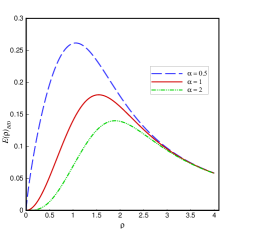
(a) $\beta=0.5$

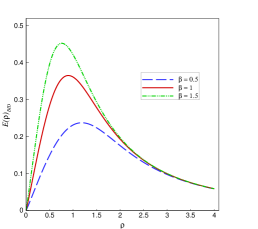
(b) $\alpha=0.6$

Figure 1: The behavior electric field $E(\rho)$ for BID black holes in (A)dS spaces versus $\rho$ for $q=b=1$

As one can see from Fig.1, in the presence of dilaton field ($\alpha\neq 0$), the electric field has zero value at $\rho=0$. For $\rho>0$, it increases smoothly until reaches a maximum value, then it decreases smoothly until goes to zero as $\rho\rightarrow\infty$. It is worth mentioning that the maximum of the electric field increases with increasing $\beta$ or decreasing $\alpha$. Besides, for $\alpha>0$, as $\beta\rightarrow\infty$, the maximum value of the electric field goes to $\rho=0$ and we have no relative maximum for $\rho>0$. In the absence of dilaton field ($\alpha=0$), the electric field has a finite value at $\rho=0$ for a finite value of $\beta$ as one may see from Eq. (32) that

$$E(\rho)\Big{|}_{\alpha=0,\,\rho=0}=\frac{q\beta}{\sqrt{q^{2}+\beta^{2}b^{4}}}$$ (36)

.

IV END black holes in AdS spacetime

In this section we examine exponential nonlinear electrodynamics coupled to the dilaton field (END) with Lagrangian (5). In this case the gravitational field equation is written as ShKa

$${\cal R}_{\mu\nu} = 2\partial_{\mu}\Phi\partial_{\nu}\Phi+\frac{1}{2}g_{\mu\nu}V(\Phi)-2e^{-2\alpha\Phi}\partial_{Y}{{\cal L}}(Y)F_{\mu\eta}F_{\nu}^{\text{ }\eta}+2\beta^{2}e^{2\alpha\Phi}\left[2Y\partial_{Y}{{\cal L}}(Y)-{{\cal L}}(Y)\right]g_{\mu\nu},$$ (37)

while the dilaton and electromagnetic field equations are still the same as those in the BID case and given by Eqs. (10) and (11), respectively. Integrating the electromagnetic field equation (11) for END Lagrangian (5), the only nonzero component of $F_{\mu\nu}$ is obtained as

$$F_{tr}=\frac{qe^{2\alpha\Phi(r)}}{r^{2}R^{2}(r)}\exp\left[-\frac{1}{2}L_{W}\left(\frac{q^{2}}{\beta^{2}r^{4}R^{4}(r)}\right)\right],$$ (38)

where $L_{W}(x)=LambertW(x)$ is the Lambert function Lambert which is a special function with definition

$$L_{W}(x)e^{L_{W}(x)}=x,$$

where $x$ is a compelex number. It is clear that $L_{W}(0)=0$, $L_{W}(e)=1$ and $L_{W}(\infty)=\infty$. The Taylor expansion of the Lambert function is

$$L_{W}(x)=\sum_{n=1}^{\infty}\frac{(-n)^{n-1}}{n!}x^{n}=x-x^{2}+\frac{3}{2}x^{3}-\frac{8}{3}x^{4}+....$$ (39)

The series expansion (39) converges for $|x|<1$. The derivative of $L_{W}(x)$ can be calculated as

$$L_{W}^{\prime}(x)=\frac{dL_{W}(x)}{dx}=\frac{L_{W}(x)}{x(1+L_{W}(x))},\qquad\qquad\qquad\rm for\ \ \emph{x}\neq 0.$$

In order to get metric and dilaton functions for this type of black holes, we use the previous ansatz (21) again. It is a matter of calculations to show that the components of the field equations (10) and (37) can be written

$$Eq_{{}_{\Phi}}=\frac{rfR}{2}\Phi^{\prime\prime}+\left(rfR^{\prime}+\frac{R}{2}\left[2f+rf^{\prime}\right]\right)\phi^{\prime}-\frac{rR}{8}\frac{dV(\Phi)}{d\Phi}+r\alpha\beta^{2}R$$

$$~{}~{}~{}~{}~{}~{}~{}~{}\times\left(\frac{q\big{(}1+2Z\big{)}}{r^{2}R^{2}\beta\sqrt{-2Z}}-1\right)e^{2\alpha\Phi(r)}=0,$$ (40)

$$Eq_{tt}=rRf^{\prime\prime}+(2rR^{\prime}+2R)f^{\prime}+r\,R\,V(\Phi)+4\beta^{2}rRe^{2\alpha\Phi}\left[1-\frac{q}{r^{2}R^{2}\beta}L_{W}\left(\frac{q^{2}}{\beta^{2}r^{4}R^{4}}\right)^{-\frac{1}{2}}\right]=0,$$

(41)

$$Eq_{rr}=4rR^{\prime\prime}f+\Big{[}2rf^{\prime}+8f\Big{]}R^{\prime}+\Big{[}rf^{\prime\prime}+2f^{\prime}+4rf{\Phi^{\prime}}^{2}+rV(\Phi)\Big{]}R+4rR\,\beta^{2}e^{2\alpha\Phi}$$

$$~{}~{}~{}~{}~{}~{}~{}~{}\times\left[1-\frac{q}{r^{2}R^{2}\beta}L_{W}\left(\frac{q^{2}}{\beta^{2}r^{4}R^{4}}\right)^{-\frac{1}{2}}\right]=0,$$ (42)

$$Eq_{\varphi\varphi}=Eq_{\theta\theta}=\Big{[}rf^{\prime}+\frac{r^{2}}{2}V(\Phi)+f\Big{]}R^{2}+\left[r^{2}fR^{\prime\prime}+\Big{(}rf^{\prime}+4f\Big{)}rR^{\prime}\right]R+r^{2}f{R^{\prime}}^{2}$$

$$~{}~{}~{}~{}~{}~{}~{}~{}~{}~{}~{}~{}~{}~{}~{}~{}~{}~{}~{}~{}-2r^{2}R^{2}\beta^{2}e^{2\alpha\Phi}\Big{[}e^{-Z}(2Z+1)-1\Big{]}+1=0,$$ (43)

where

$$Z=-\frac{1}{2}L_{W}\left(\frac{q^{2}}{\beta^{2}r^{4}R^{4}}\right).$$ (44)

Subtracting Eq. (41) from Eq. (42), and using the ansatz (21) we arrive at Eq. (22). Thus the dilaton field is again given by Eq. (23). This implies that the nonlinearity does not affect the dilaton field. Having ansatz (21) and the dilaton field (23) in hand, we can obtain the metric function $f(r)$ by solving Eq. (43). We find

$$f(r) = -\frac{\Lambda r^{2}}{3}\left(1-\frac{b}{r}\right)^{\gamma}+\frac{1}{r(\alpha^{2}+1)-b}\left(1-\frac{b}{r}\right)^{1-\gamma}$$

$$\times\left[C_{2}+r(\alpha^{2}+1)-2\beta^{2}(\alpha^{2}+1)\int r^{2}\left(1-\frac{b}{r}\right)^{2\gamma}\left[1+\sqrt{\eta}\left(\sqrt{L_{W}(\eta)}-\frac{1}{\sqrt{L_{W}(\eta)}}\right)\right]dr\right],$$

where $C_{2}$ is an integration constant related to the mass of the black hole. In the absence of dilaton field ($\alpha=0$), the above solution reduces to

$$f(r) = 1+\frac{C_{2}}{r}-\frac{\Lambda r^{2}}{3}-\frac{2\beta^{2}r^{2}}{3}-\frac{2\beta q}{r}\bigintsss\Bigg{[}\sqrt{L_{W}\left(\frac{q^{2}}{r^{4}\beta^{2}}\right)}-\frac{1}{\sqrt{L_{W}\left(\frac{q^{2}}{r^{4}\beta^{2}}\right)}}\Bigg{]}\,dr,$$ (46)

which is the metric AdS black holes in in the presence of EN electrodynamics AsympDrHendi . The series expansion of (46) for large $\beta$ becomes

$$f(r)=1+\frac{C_{2}}{r}+{\frac{{q}^{2}}{{r}^{2}}}-\frac{\Lambda r^{2}}{3}-{\frac{{q}^{4}}{20\,{r}^{6}{\beta}^{2}}}+{\frac{5{q}^{6}}{216\,{r}^{10}{\beta}^{4}}}+O\left(\frac{1}{{\beta}^{6}}\right).$$ (47)

For $\beta\rightarrow\infty$, the above solution reduces to RN-AdS black hole. Now, we substitute the metric function (IV) in the all components of the field equations (IV)-(43). We find that in order to fully satisfy all field equations, we should have the following conditions for $q$, $\beta$ and $C_{{}_{2}}$

$$\frac{b+C_{2}}{2(\alpha^{2}+1)}+\frac{q^{2}}{r\,b\,\eta}\left[1+\sqrt{\eta}\left(\sqrt{L_{W}(\eta)}-\frac{1}{\sqrt{L_{W}(\eta)}}\right)\right]\Big{(}r(\alpha^{2}+1)-b\Big{)}$$

$$-\beta^{2}\int r^{2}\left(1-\frac{b}{r}\right)^{2\gamma}\left[1+\sqrt{\eta}\left(\sqrt{L_{W}(\eta)}-\frac{1}{\sqrt{L_{W}(\eta)}}\right)\right]dr=0.$$ (48)

It is interesting to check the limiting case of (IV) for large $\beta$,

$$C_{2} = -\frac{b^{2}+(1+\alpha^{2})q^{2}}{b}+O\left(\frac{1}{\beta^{2}}\right),$$ (49)

which is again the condition in case of AdS dilaton balck holes coupled to the linear Maxwell gauge field gao1 . Combining condition (IV) with solution (IV), we find the final form of the metric function, which fully satisfy the field equations, for END black holes in the background of (A)dS spaces as

$$f(r)=-\frac{\Lambda r^{2}}{3}\left(1-\frac{b}{r}\right)^{\gamma}+\Bigg{\{}1-\frac{2q^{2}(\alpha^{2}+1)}{r\,b\,\eta}\left[1+\sqrt{\eta}\Bigg{(}\sqrt{L_{W}(\eta)}-\frac{1}{\sqrt{L_{W}(\eta)}}\Bigg{)}\right]\Bigg{\}}\left(1-{\frac{b}{r}}\right)^{1-\gamma}$$ (50)

In order to calculate the explicit form of the electric field for END-AdS black hole, we substitute the dilaton field (23) in the electromagnetics tensor (38). We find

$$E(r)=\frac{q}{r^{2}}\sqrt{\frac{L_{W}(\eta)}{\eta}}.$$ (51)

where $\eta$ is given by (25). When $\alpha=0$, the electric field of black holes in the presence of EN electrodynamics is restored AsympDrHendi . It is worthy to note that the electric field (51) differs from the case of non-asymptotically (A)dS dilaton black holes in the presence of EN electrodynamics ShKa . Also, the expansion of Eq. (51) for large $\beta$, yields

$$E(r)=\frac{q}{r^{2}}-\frac{q^{3}}{2r^{6}\beta^{2}}\left(1-\frac{b}{r}\right)^{-2\gamma}+O\left(\frac{1}{\beta^{4}}\right).$$ (52)

when $\beta\rightarrow\infty$, the electric field does not depend on the dilaton field and reduces to the electric field of AdS dilaton black hole SheAdS .

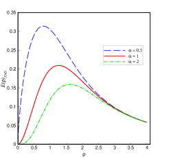
(a) $\beta=0.5$

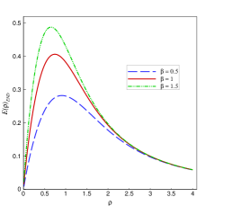
(b) $\alpha=0.6$

Figure 2: The behavior of electric field $E(\rho)$ for END black holes in (A)dS space versus $\rho$ for $q=b=1$

In order to have better understanding on the behavior of the electric field, we plot Fig. 2. Again, our solution does not exist in the range $0<r<b$, so we use the new radial coordinate (34) to exclude this region from the spacetime. In Fig. 2, $E(\rho)$ is plotted versus $\rho$ for different values of $\alpha$ and $\beta$. From this figure we see a new behaviour for the electric field of END black holes in AdS spaces. As one can see the electric field vanishes at $\rho=0$ and has a maximum value at some $\rho=\rho_{0}>0$. The maximum point of the electric field depends on the parameters. Indeed, for a fixed value of $\beta$ the maximum of electric field increase as $\alpha$ decrease (fig. 2(a)). Also, in the presence of the dilaton field ($\alpha>0$), by increasing the nonlinear parameter $\beta$, this maximum increases, while its position shifted to the point $\rho_{0}\rightarrow 0$ (fig. 2(b)).

V LND black holes in AdS spacetime

In this section we would like to construct black hole solution for Logarithmic nonlinear electrodynamics coupled to dilaton field in the background of (A)dS spaces. Variation with respect to both gravitational and dilaton fields yield the following field equations ShN

$${\cal R}_{\mu\nu}^{LND} = 2\partial_{\mu}\Phi\partial_{\nu}\Phi+\frac{1}{2}g_{\mu\nu}V(\Phi)+2e^{-2\alpha\Phi}\partial_{Y}{{\cal L}}(Y)F_{\mu\eta}F_{\nu}^{\text{ }\eta}-4\beta^{2}e^{2\alpha\Phi}\left[2Y\partial_{Y}{{\cal L}}(Y)-{{\cal L}}(Y)\right]g_{\mu\nu},\qquad$$ (53)

$$\nabla^{2}\Phi = \frac{1}{4}\frac{\partial V}{\partial\Phi}-4\alpha\beta^{2}e^{2\alpha\Phi}\left[2{Y}\partial_{Y}{{\cal L}}(Y)-{\cal L}(Y)\right].$$ (54)

Note that the equation of motion for the electrodynamics still obeys Eq. (11) with Lagrangian given in (6), and considering metric (8), one can show that it has the following solution

$$F_{tr}=\frac{2\,q\,e^{2\alpha\Phi(r)}}{r^{2}R^{2}(r)}\left(1+\sqrt{1+\frac{q^{2}}{\beta^{2}\,r^{4}\,R^{4}(r)}}\right)^{-1}.$$ (55)

Substituting the metric (8) and the electric field (55) in the field equations (53) and (54), we can write these equations as

$$Eq_{{}_{\Phi}}=\frac{rfR}{2}\Phi^{\prime\prime}+\left(rfR^{\prime}+\frac{R}{2}\left[2f+rf^{\prime}\right]\right)\phi^{\prime}-\frac{rR}{8}\frac{dV(\Phi)}{d\Phi}-2r\alpha\beta^{2}R$$

$$~{}~{}~{}~{}~{}~{}~{}~{}\times\Bigg{\{}\ln\Big{(}1+W\Big{)}-\left(1+\sqrt{1+\frac{q^{2}}{r^{4}R^{4}\beta^{2}}}\right)W\Bigg{\}}e^{2\alpha\Phi(r)}=0$$ (56)

$$Eq_{tt}=rRf^{\prime\prime}+\Big{[}2rR^{\prime}+2R\Big{]}f^{\prime}+r\,R\,V(\Phi)+8\beta^{2}rRe^{2\alpha\Phi}$$

$$~{}~{}~{}~{}~{}~{}~{}~{}~{}\times\Bigg{\{}\ln(W+1)-2\left(\frac{\frac{W\beta^{2}r^{4}R^{4}}{1+W}\sqrt{1+\frac{q^{2}}{r^{4}R^{4}\beta^{2}}}+\frac{q^{2}}{2}}{\beta^{2}r^{4}R^{4}\sqrt{1+\frac{q^{2}}{r^{4}R^{4}\beta^{2}}}+\frac{q^{2}}{2}}\right)\Bigg{\}}=0,$$ (57)

$$Eq_{rr}=4rR^{\prime\prime}f+\Big{[}2rf^{\prime}+8f\Big{]}R^{\prime}+\Big{[}rf^{\prime\prime}+2f^{\prime}+4rf{\Phi^{\prime}}^{2}+rV(\Phi)\Big{]}R-16\beta^{2}rRe^{2\alpha\Phi}$$

$$~{}~{}~{}~{}~{}~{}~{}~{}~{}\times\Bigg{\{}-\frac{1}{2}\ln(W+1)+\left(\frac{\frac{W\beta^{2}r^{4}R^{4}}{1+W}\sqrt{1+\frac{q^{2}}{r^{4}R^{4}\beta^{2}}}+\frac{q^{2}}{2}}{\beta^{2}r^{4}R^{4}\sqrt{1+\frac{q^{2}}{r^{4}R^{4}\beta^{2}}}+\frac{q^{2}}{2}}\right)\Bigg{\}}=0,$$ (58)

$$Eq_{\varphi\varphi}=Eq_{\theta\theta}=\Big{[}rf^{\prime}+\frac{r^{2}}{2}V(\Phi)+f\Big{]}R^{2}+\left[r^{2}fR^{\prime\prime}+\Big{(}rf^{\prime}+4f\Big{)}rR^{\prime}\right]R$$

$$~{}~{}~{}~{}~{}~{}~{}~{}~{}~{}~{}~{}~{}~{}~{}~{}~{}~{}~{}~{}+r^{2}f{R^{\prime}}^{2}+4r^{2}R^{2}\beta^{2}e^{2\alpha\Phi}\left(\ln(W+1)-\frac{2W}{W+1}\right)-1=0,$$ (59)

where

$$W=-\frac{q^{2}}{r^{4}R^{4}\beta^{2}}\left(1+\sqrt{1+\frac{q^{2}}{r^{4}R^{4}\beta^{2}}}\right)^{-2}.$$ (60)

Following our approach in the previous sections, we substrate Eq. (V) from Eq. (V) and again arrive at equation (20). After using ansatz (21), we find Eq. (22), which admits a solution in the form (23). Inserting ansatz (21), the dilaton field (23) and the potential (7) in Eq. (V), we obtain the following solution

$$f(r) = -\frac{\Lambda r^{2}}{3}\left(1-\frac{b}{r}\right)^{\gamma}+\frac{1}{r(\alpha^{2}+1)-b}\left(1-\frac{b}{r}\right)^{1-\gamma}$$ (61)

$$\times\Bigg{\{}C{{}_{3}}+r(\alpha^{2}+1)-4q^{2}(\alpha^{2}+1)\int\frac{1}{r^{2}\eta}\left[\frac{\eta}{1+\sqrt{1+\eta}}+\ln\left(\frac{2}{1+\sqrt{1+\eta}}\right)\right]dr\Bigg{\}}.$$

Here $\eta$ is again given by (25) and $C_{3}$ is a constant of integration. When $\alpha=0$, the above solution reduces to

$$f(r) = 1+\frac{C_{3}}{r}-\frac{\Lambda r^{2}}{3}-\frac{4}{r}\bigintsss\Bigg{\{}\frac{q^{2}}{r^{2}}\frac{1}{1+\sqrt{1+\frac{q^{2}}{r^{4}\beta^{2}}}}+r^{2}\beta^{2}\ln\Bigg{(}\frac{2}{1+\sqrt{1+\frac{q^{2}}{r^{4}\beta^{2}}}}\Bigg{)}\Bigg{\}}\,dr,$$ (62)

which is the metric of AdS black holes in in the presence of LN electrodynamics AsympDrHendi . The series expansion of (62) for large $\beta$ becomes

$$f(r)=1+\frac{C_{3}}{r}+{\frac{{q}^{2}}{{r}^{2}}}-\frac{\Lambda r^{2}}{3}-{\frac{{q}^{4}}{40\,{r}^{6}{\beta}^{2}}}+{\frac{{q}^{6}}{216\,{r}^{10}{\beta}^{4}}}+O\left(\frac{1}{{\beta}^{6}}\right).$$ (63)

In the liming case where $\beta\rightarrow\infty$, the above solution reduces to RN-AdS black hole. Inserting the metric function (61) in the field Eqs. (V)-(V), after a time-consuming calculations, we find a relation between constants $q$, $\beta$, $C_{3}$ and the integration part of solution (61) as

$$\frac{b+C_{3}}{4(\alpha^{2}+1)}+\frac{q^{2}}{r\,b\,\eta}\left[\frac{\eta}{1+\sqrt{1+\eta}}+\ln\left(\frac{2}{1+\sqrt{1+\eta}}\right)\right]\Big{(}r(\alpha^{2}+1)-b\Big{)}$$

$$-q^{2}\int\frac{1}{r^{2}\eta}\left[\frac{\eta}{1+\sqrt{1+\eta}}+\ln\left(\frac{2}{1+\sqrt{1+\eta}}\right)\right]dr=0,$$ (64)

Again expanding the above condition for large $\beta$, we find

$$C_{3}=-\frac{b^{2}+(1+\alpha^{2})q^{2}}{b}+O\left(\frac{1}{\beta^{2}}\right),$$ (65)

Combining condition (V) with solution (61), we arrive at the final form of the metric function for LND black holes in (A)dS spaces as

$$f(r) = -\frac{\Lambda r^{2}}{3}\left(1-\frac{b}{r}\right)^{\gamma}+\Bigg{\{}1-\frac{4q^{2}(\alpha^{2}+1)}{r\,b\,\eta}\left[\frac{\eta}{1+\sqrt{1+\eta}}+\ln\left(\frac{2}{1+\sqrt{1+\eta}}\right)\right]\Bigg{\}}\left(1-{\frac{b}{r}}\right)^{1-\gamma}.$$ (66)

Now we back to the calculate the explicit form of the electric field. One can show that the combination of dilaton field, Eq. (21) and Eq. (55) results the electric field for this type of black hole as

$$E(r)=\frac{2\,q}{r^{2}}\frac{1}{1+\sqrt{1+\eta}}.$$ (67)

In the absence of dilaton field ($\alpha=0$), this expression for the electric field reduces to one presented in AsympDrHendi . Let us note that in the large limit of nonlinear parameter $\beta$, the electric field becomes

$$E(r)=\frac{q}{r^{2}}+\frac{q^{3}}{4\,r^{6}\,\beta^{2}}\left(1-\frac{b}{r}\right)^{2\gamma}+O\left(\frac{1}{\beta^{4}}\right).$$ (68)

It is clear that the first term in the above relation is the electric field of EMd black holes in AdS spaces SheAdS which is independent of dilaton coupling $\alpha$, and the second term is the leading order correction term which appears due to the nonlinearity of the electrodynamic field.

Let us note that at $\rho=0$ the electric field becomes zero like the two previous nonlinear electrodynamics. The behavior of the electric field respect to $\rho$ is plotted in Fig. 3. From this figure, we observe that in the presence of the dilaton field, the behaviour of the electric field is similar to the electric field of END and BID black holes in the previous sections.

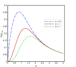
(a) $\beta=0.5$

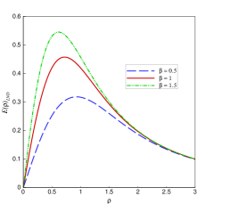
(b) $\alpha=0.6$

Figure 3: The behavior of $E(\rho)$ for LND black holes in (A)dS space versus $\rho$ for $q=b=1$

VI Discussion

Now, we want to study the casual structure and physical properties of the obtained solutions. Let us remember that the metric function of asymptotically (Ad)S black holes in EMd gravity has the following form SheAdS

$$f(r)_{\rm EMd}=\left(1-\frac{c}{r}\right)\left(1-{\frac{b}{r}}\right)^{1-\gamma}-\frac{\Lambda r^{2}}{3}\left(1-\frac{b}{r}\right)^{\gamma},$$ (69)

where the two constants $c$ and $b$ are satisfied $q^{2}(\alpha^{2}+1)=bc$. Expanding the obtained solutions in Eqs. (30), (50) and (66) for large $\beta$, we find

$$f(r)_{\rm BID} = f(r)_{\rm END}=f(r)_{\rm EMd}+\frac{q^{4}(\alpha^{2}+1)}{4\,br^{5}\beta^{2}}\left(1-{\frac{b}{r}}\right)^{1-3\gamma}+O\left(\frac{1}{\beta^{4}}\right)$$ (70)

$$f(r)_{\rm LND}=f(r)_{\rm EMd}+\frac{q^{4}(\alpha^{2}+1)}{8\,br^{5}\beta^{2}}\left(1-{\frac{b}{r}}\right)^{1-3\gamma}+O\left(\frac{1}{\beta^{4}}\right)$$

It is obvious that for $r\rightarrow\infty$, the dominant term in all solutions is $-{\Lambda r^{2}}/{3}$, which guarantees that the asymptotic behavior of the metric function is (A)dS for ($\Lambda<0$) $\Lambda>0$. The expansion of these solutions in the absence of dilaton field ($\alpha=0$) and for $r\rightarrow\infty$ can be written as

$$f(r)_{\rm BID}=f(r)_{\rm END}=-\frac{\Lambda r^{2}}{3}+\left(1-{\frac{b}{r}}\right)\Bigg{\{}1-\frac{c}{r}+\frac{q^{4}}{4br^{5}\beta^{2}}-\frac{q^{6}}{8br^{9}\beta^{4}}\Bigg{\}}+O\left(\frac{1}{\beta^{6}}\right),$$

$$f(r)_{\rm LND}=-\frac{\Lambda r^{2}}{3}+\left(1-{\frac{b}{r}}\right)\Bigg{\{}1-\frac{c}{r}+\frac{q^{4}}{8br^{5}\beta^{2}}-\frac{q^{6}}{24br^{9}\beta^{4}}\Bigg{\}}+O\left(\frac{1}{\beta^{6}}\right).$$ (71)

Now, we are going to investigate the geometric nature of the solutions. The existence of singularity and horizon ensure that solutions are intrinsically black holes. To cover all the spacetime, we prefer to continue with the new coordinate $\rho$. One can compute the Ricci and Kretschmann scalars as

$$Ricci = -\left(1+\frac{b^{2}}{\rho^{2}}\right)f^{\prime\prime}+\Bigg{[}-4\rho(b^{2}+\rho^{2})R^{\prime}+(b^{2}-4\rho^{2})R\Bigg{]}\frac{f^{\prime}}{R\rho^{3}}+\frac{2}{R^{2}(b^{2}+\rho^{2})}$$

$$+\Bigg{[}-4\rho(b^{2}+\rho^{2})R^{\prime\prime}R-2\rho(b^{2}+\rho^{2}){R^{\prime}}^{2}+4(b^{2}-3\rho^{2})R^{\prime}R-\frac{2\rho^{3}R^{2}}{b^{2}+\rho^{2}}\Bigg{]}\frac{f}{R^{2}\rho^{3}}$$

$$R_{\mu\nu\rho\sigma}R^{\mu\nu\rho\sigma} = \frac{(b^{2}+\rho^{2})^{2}}{\rho^{4}}{f^{\prime\prime}}^{2}+\Bigg{[}4(b^{2}+\rho^{2})^{2}{R^{\prime}}^{2}+8\rho(b^{2}+\rho^{2})RR^{\prime}+\frac{(b^{4}+4\rho^{4})R^{2}}{\rho^{2}}\Bigg{]}\frac{{f^{\prime}}^{2}}{\rho^{4}R^{2}}$$ (72)

$$+\Bigg{\{}-\frac{2b^{2}(b^{2}+\rho^{2})f^{\prime\prime}}{\rho^{5}}+8\Big{[}\rho(b^{2}+\rho^{2})R^{\prime\prime}-(b^{2}-2\rho^{2})R^{\prime}\Big{]}\ \Big{(}(b^{2}+\rho^{2})R^{\prime}+\rho R\Big{)}\frac{f}{\rho^{5}R^{2}}\Bigg{\}}f^{\prime}$$

$$+\Bigg{\{}\frac{4\rho(b^{2}+\rho^{2})^{2}{R^{\ \prime}}^{4}}{R}+16\rho^{3}(b^{2}+\rho^{2}){R^{\prime}}^{3}+\frac{16\rho^{5}R^{2}R^{\prime}}{(b^{2}+\rho^{2})}+\frac{4\rho^{6}R^{3}}{(b^{2}+\rho^{2})^{2}}$$

$$+8\Bigg{[}\rho^{2}(b^{2}+\rho^{2})^{2}{R^{\prime\prime}}^{2}-2\rho(b^{2}+\rho^{2})(b^{2}-2\rho^{2})R^{\prime}R^{\prime\prime}+(b^{4}-4b^{2}\rho^{2}+7\rho^{4}){R^{\prime}}^{2}\Bigg{]}R\Bigg{\}}\frac{f^{2}}{\rho^{6}R^{3}}$$

$$+\left(-8(b^{2}+\rho^{2}){R^{\prime}}^{2}-16\rho RR^{\prime}-\frac{8\rho^{2}R^{2}}{b^{2}+\rho^{2}}\right)\frac{f}{(b^{2}+\rho^{2})\rho^{2}R^{4}}+\frac{4}{(b^{2}+\rho^{2})^{2}R^{4}}$$

where the prime indicates the derivative with respect to $\rho$. Also, $R=R(\rho)$ and $f=f(\rho)$ where may find them as

$$R(\rho) = \left(1-\frac{b}{\sqrt{b^{2}+\rho^{2}}}\right)^{\frac{\gamma}{2}}$$ (73)

$$f(\rho)_{BID} = -\left(1-\frac{b}{\sqrt{b^{2}+\rho^{2}}}\right)^{\gamma}\frac{(b^{2}+\rho^{2})\Lambda}{3}+\left(1-\frac{b}{\sqrt{b^{2}+\rho^{2}}}\right)^{1-\gamma}$$ (74)

$$\times\Bigg{\{}1-\frac{2\beta^{2}(\alpha^{2}+1)}{b}(b^{2}+\rho^{2})^{\frac{3}{2}}\left(1-\frac{b}{\sqrt{b^{2}+\rho^{2}}}\right)^{2\gamma}\left[\sqrt{1+\eta_{\rho}}-1\right]\Bigg{\}}$$

$$f(\rho)_{END} = -\left(1-\frac{b}{\sqrt{b^{2}+\rho^{2}}}\right)^{\gamma}\frac{(b^{2}+\rho^{2})\Lambda}{3}+\left(1-\frac{b}{\sqrt{b^{2}+\rho^{2}}}\right)^{1-\gamma}$$ (75)

$$\times\Bigg{\{}1-\frac{2q^{2}(\alpha^{2}+1)}{\,b\,\eta_{\rho}\sqrt{b^{2}+\rho^{2}}}\left[1+\sqrt{\eta_{\rho}}\Bigg{(}\sqrt{L_{W}(\eta_{\rho})}-\frac{1}{\sqrt{L_{W}(\eta_{\rho})}}\Bigg{)}\right]\Bigg{\}}$$

$$f(\rho)_{LND} = -\left(1-\frac{b}{\sqrt{b^{2}+\rho^{2}}}\right)^{\gamma}\frac{(b^{2}+\rho^{2})\Lambda}{3}+\left(1-\frac{b}{\sqrt{b^{2}+\rho^{2}}}\right)^{1-\gamma}$$ (76)

$$\times\Bigg{\{}1-\frac{4q^{2}(\alpha^{2}+1)}{b\,\eta_{\rho}\sqrt{b^{2}+\rho^{2}}}\left[\frac{\eta_{\rho}}{1+\sqrt{1+\eta_{\rho}}}+\ln\left(\frac{2}{1+\sqrt{1+\eta_{\rho}}}\right)\right]\Bigg{\}}$$

where

$$\eta_{\rho}=\frac{q^{2}}{\beta^{2}(b^{2}+\rho^{2})^{2}}\left(1-\frac{b}{\sqrt{b^{2}+\rho^{2}}}\right)^{-2\gamma}$$ (77)

It is a matter of calculation to show that these scalars diverge in the vicinity of the origin, namely

$$\lim\limits_{\rho\rightarrow 0}Ricci = \infty,$$

$$\lim\limits_{\rho\rightarrow 0}R_{\mu\nu\rho\sigma}R^{\mu\nu\rho\sigma} = \infty.$$

These confirm that the spacetime associated with the solutions has a singularity at the origin ($\rho=0$). Also, it can be shown that in large distances and for various values of $\alpha$, the Ricci and Kretschmann scalars are $N\Lambda$, where $N$ is a positive number, so it guarantees that the asymptotical behavior of these solutions is (A)dS for $\Lambda<0$ ($\Lambda>0$). Now, we focus on the existence of horizon.

In order to find the location of all horizons one should solve $f(\rho=\rho_{+})$=0. Due to the complexity of the obtained metric functions, it is not possible to solve this equation analytically. To have better understanding on the nature of horizons, we plot $f(\rho)$ versus $\rho$ for different metric parameters.

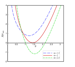
(a) $f(\rho)_{{}_{\rm BID}}$ for $q=0.97$

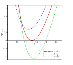
(b) $f(\rho)_{{}_{\rm END}}$ for $q=0.87$

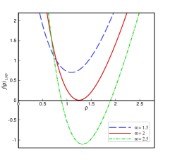
(c) $f(\rho)_{{}_{\rm LND}}$ for $q=0.81$

Figure 4: The behavior of $f(\rho)$ versus $\rho$ for $\beta=0.5$, $\Lambda=-3$ and $b=1$.

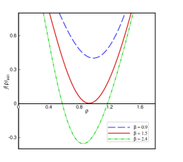
(a) $f(\rho)_{{}_{\rm BID}}$ for $q=1.13$

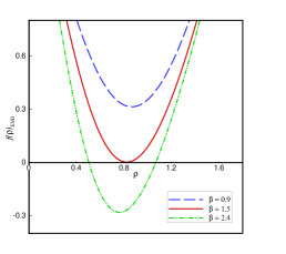
(b) $f(\rho)_{{}_{\rm END}}$ for $q=1.064$

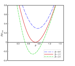
(c) $f(\rho)_{{}_{\rm LND}}$ for $q=1$

Figure 5: The behavior of $f(\rho)$ versus $\rho$ for $\alpha=1.1$, $\Lambda=-3$ and $b=1$.

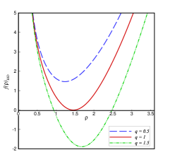
(a) $f(\rho)_{{}_{\rm BID}}$ for $\beta=0.47$

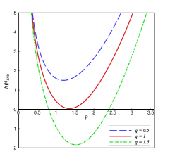
(b) $f(\rho)_{{}_{\rm END}}$ for $\beta=0.33$

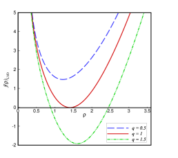
(c) $f(\rho)_{{}_{\rm LND}}$ for $\beta=0.29$

Figure 6: The behavior of $f(\rho)$ versus $\rho$ for $\alpha=2$, $\Lambda=-3$ and $b=1$.

According to these figures, the existence of horizons and their numbers are crucially depend on the values of the metric parameters. By suitable choices of the different parameters, one can see that since $f(\rho)$ is positive near the origin as well as large distances, the obtained solution may represent black holes with two horizons, an extreme black hole or naked singularity depending on the parameters. To be more precise, the effects of parameters are plotted in different figures. Fig. 4 shows that by fixing other metric parameters, increasing of $\alpha$ may increase the number of horizons in all presented theories. From Fig. 5, one may realize that, when other metric parameters are fixed, a direct relation between the increase of the nonlinear parameter $\beta$ and the number of horizon stands for all three metric functions. Also, by fixing other parameters, the same behavior is seen for electric charge $q$ in Fig. 6. It is worth noting that the effect of changes in metric parameters on the number of horizons of BID-(A)dS, END-(A)dS and LND-(A)dS black holes is quite contrary to the their counterparts in non-(A)dS spacetime. As mentioned in Shey2 ; ShKa ; ShN for non-(A)dS dilaton black holes with nonlinear electrodynamics, by fixing other metric parameters, decreasing of the electric charge parameter $q$, or nonlinear parameter $\beta$ or dilaton coupling constant $\alpha$ may increase the number of horizon, but our solutions treat differently in this regard.

VII Closing remarks

Till now exact analytical solutions of Einstein-dilaton gravity in the presence of nonlinear electrodynamics and in the background of (A)dS spaces have not been constructed. In this paper, we constructed three classes of asymptotically AdS dilaton black holes solutions in the presence of nonlinear electrodynamics. We have considered three type of nonlinear electrodynamics, namely BID, END and LND field. For this purpose, we utilized a combination of three Liouville-type dilaton potential. We found the metric functions, electric field and dilaton field and studied their behaviour for three class of solutions. We observed that the nonlinearity of the gauge field do not affect the dilaton field, and for $r\rightarrow\infty$ ($\rho\rightarrow\infty$), the dilaton field goes to zero. We proved that our solution has a singularity at $\rho=0$ ($r=b$), which depending on the value of the metric function, it can be covered by the one or two horizon. Also, we realized that the number of horizon increases by increasing nonlinear parameter $\beta$, electric charge $q$ or dilaton coupling constant $\alpha$. We studied the behavior of the electric field of all three nonlinear electrodynamics. Interestingly, we found out that in the presence of the dilaton field, the electric field has a strange behaviour. Indeed, it vanishes at $\rho=0$ and increases until reaches a maximum value at $\rho=\rho_{0}$ and goes to zero smoothly as $r\rightarrow\infty$ ($\rho\rightarrow\infty$). We observed that the electric field is zero at singularity and increases smoothly until reaches a maximum value, then it decreases smoothly until goes to zero as $r\rightarrow\infty$ ($\rho\rightarrow\infty$). The maximum value of the electric field increases with increasing the nonlinear parameter $\beta$ or decreasing the dilaton coupling $\alpha$ and is shifted to the origin in the absence of either dilaton field ($\alpha=0$) or nonlinear gauge field ($\beta\rightarrow\infty$). It seems that the coupling of the nonlinear gauge field with the dilaton field in the background of (A)dS space leads to such an unfamiliar behavior. However, the physical reason for this behaviour and its origin deserves further investigations and we leave them for the future works. It would be also interesting to carry out the investigation on the thermodynamics of the obtained solutions. One may also interested in generalizing these four dimensional static and spherically symmetric solutions to the rotating and higher dimensional cases with other horizon topology. We leave these issues for future works.