Sampled-data implementation of derivative-dependent control using artificial delays

Abstract

We study a sampled-data implementation of linear controllers that depend on the output and its derivatives. First, we consider an LTI system of relative degree $r\geq 2$ that can be stabilized using $r-1$ output derivatives. Then, we consider PID control of a second order system. In both cases, the Euler approximation is used for the derivatives giving rise to a delayed sampled-data controller. Given a derivative-dependent controller that stabilizes the system, we show how to choose the parameters of the delayed sampled-data controller that preserves the stability under fast enough sampling. The maximum sampling period is obtained from LMIs that are derived using the Taylor’s expansion of the delayed terms with the remainders compensated by appropriate Lyapunov-Krasovskii functionals. Finally, we introduce the event-triggering mechanism that may reduce the amount of sampled control signals used for stabilization.

I Introduction

Control laws that depend on output derivatives are used to stabilize systems with relative degrees greater than one. To estimate the derivatives, which can hardly be measured directly, one can use the Euler approximation $\dot{y}\approx(y(t)-y(t-\tau))/\tau$. This replaces the derivative-dependent control with the delay-dependent one [2, 3, 4, 5]. It has been shown in [6] that such approximation preserves the stability if $\tau>0$ is small enough. Similarly, the output derivative in PID controller can be replaced by its Euler approximation. The resulting controller was studied in [7] and [8] using the frequency domain analysis.

In this paper, we study sampled-data implementation of the delay-dependent controllers. For double-integrators, this has been done in [9] using complete Lyapunov-Krasovskii functionals with a Wirtinger-based term and in [10] via impulsive system representation and looped-functionals. Both methods lead to complicated linear matrix inequalities (LMIs) containing many decision variables. In this paper, we obtain simpler LMIs for more general systems and prove their feasibility for small enough sampling periods.

A simple Lyapunov-based method for delay-induced stabilization was proposed in [11, 12]. The key idea is to use the Taylor’s expansion of the delayed terms with the remainders in the integral form that are compensated by appropriate terms in the Lyapunov-Krasovskii functional. This leads to simple LMIs feasible for small delays if the derivative-dependent controller stabilizes the system.

In this paper, we study sampled-data implementation of two types of derivative-dependent controllers. In Section II, we consider an LTI system of relative degree $r\geq 2$ that can be stabilized using $r-1$ output derivatives. In Section III, we consider PID control of a second order system. In both cases, the Euler approximation is used for the derivatives giving rise to a delayed sampled-data controller. Assuming that the derivative-dependent controller exponentially stabilizes the system with a decay rate $\alpha^{\prime}>0$, we show how to choose the parameters of its sampled-data implementation that exponentially stabilizes the system with any decay rate $\alpha<\alpha^{\prime}$ if the sampling period is small enough. The maximum sampling period is obtained from LMIs that are derived using the ideas of [11, 12]. Finally, we introduce the event-triggering mechanism that may reduce the amount of sampled control signals used for stabilization [13, 14, 15, 16, 17]. In the preliminary paper [1], we studied delayed sampled-data control for systems with relative degree two.

Notations: $\mathbb{N}_{0}=\mathbb{N}\cup\{0\}$, $\mathbf{1}_{r}=[1,1,\ldots,1]^{T}\in\mathbb{R}^{r}$, $I_{l}\in\mathbb{R}^{l\times l}$ is the identity matrix, $\otimes$ stands for the Kronecker product, $\lfloor x\rfloor=\max\{n\!\in\!\mathbb{N}\mid n\!\leq\!x\}$ for $x\in\mathbb{R}$, $\operatorname{col}\{a_{1},\ldots,a_{r}\}$ denotes the column vector composed from the vectors $a_{1},\ldots,a_{r}$. For $p\in\mathbb{R}$, $f(h)=O(h^{p})$ if there exist positive $M$ and $h_{0}$ such that $|f(h)|\leq Mh^{p}$ for $h\in(0,h_{0})$.

Auxiliary lemmas

Lemma 1 (Exponential Wirtinger inequality [18])

Let $f\in\mathcal{H}^{1}(a,b)$ be such that $f(a)=0$ or $f(b)=0$. Then

$$\textstyle\int_{a}^{b}e^{2\alpha t}f^{T}(t)Wf(t)\,dt\\ \textstyle\leq e^{2|\alpha|(b-a)}\frac{4(b-a)^{2}}{\pi^{2}}\int_{a}^{b}e^{2\alpha t}\dot{f}^{T}(t)W\dot{f}(t)\,dt$$

for any $\alpha\in\mathbb{R}$ and $0\leq W\in\mathbb{R}^{n\times n}$.

Lemma 2 (Jensen’s inequality [19])

Let $\rho\colon[a,b]\to[0,\infty)$ and $f\colon[a,b]\to\mathbb{R}^{n}$ be such that the integration concerned is well-defined. Then for any $0<Q\in\mathbb{R}^{n\times n}$,

$$\textstyle\left[\int_{a}^{b}\rho(s)f(s)\,ds\right]^{T}Q\left[\int_{a}^{b}\rho(s)f(s)\,ds\right]\leq\\ \textstyle\int_{a}^{b}\rho(s)\,ds\int_{a}^{b}\rho(s)f^{T}(s)Qf(s)\,ds.$$

II Derivative-dependent control using discrete-time measurements

Consider the LTI system

$$\begin{aligned} \dot{x}(t)&=Ax(t)+Bu(t),\\ y(t)&=Cx(t),\end{aligned}\qquad x\in\mathbb{R}^{n},u\in\mathbb{R}^{m},y\in\mathbb{R}^{l}$$ (1)

with relative degree $r\geq 2$, i.e.,

$$CA^{i}B=0,\quad i=0,1,\ldots,r-2,\quad CA^{r-1}B\neq 0.$$ (2)

Relative degree is how many times the output $y(t)$ needs to be differentiated before the input $u(t)$ appears explicitly. In particular, (2) implies

$$y^{(i)}=CA^{i}x,\quad i=0,1,\ldots,r-1.$$ (3)

To prove (3), note that it is trivial for $i=0$ and, if it has been proved for $i<r-1$, it holds for $i+1$:

$$\textstyle y^{(i+1)}=\left(y^{(i)}\right)^{\prime}\stackrel{{\scriptstyle\eqref{y'}}}{{=}}(CA^{i}x)^{\prime}=CA^{i}[Ax+Bu]\stackrel{{\scriptstyle\eqref{CB=0}}}{{=}}CA^{i+1}x.$$

For LTI systems with relative degree $r$, it is common to look for a stabilizing controller of the form

$$u(t)=\bar{K}_{0}y(t)+\bar{K}_{1}\dot{y}(t)+\ldots+\bar{K}_{r-1}y^{(r-1)}(t)$$ (4)

with $\bar{K}_{i}\in\mathbb{R}^{m\times l}$ for $i=0,\ldots,r-1$.

Remark 1

The control law (4) essentially reduces the system’s relative degree from $r\geq 2$ to $r=1$. Indeed, the transfer matrix of (1) has the form

$$\textstyle W(s)=\frac{\beta_{r}s^{n-r}+\cdots+\beta_{n}}{s^{n}+\alpha_{1}s^{n-1}+\cdots+\alpha_{n}}$$

with $\beta_{r}=CA^{r-1}B\neq 0$. Taking $u(t)=K_{0}^{\prime}u_{0}(t)+K_{1}^{\prime}\dot{u}_{0}(t)+\cdots+K_{r-1}^{\prime}u_{0}^{(r-1)}(t)$, one has

$$\textstyle\tilde{y}(s)=\frac{(\beta_{r}s^{n-r}+\cdots+\beta_{n})(K_{r-1}^{\prime}s^{r-1}+\cdots+K_{0}^{\prime})}{s^{n}+\alpha_{1}s^{n-1}+\cdots+\alpha_{n}}\tilde{u}_{0}(s),$$

where $\tilde{y}$ and $\tilde{u}_{0}$ are the Laplace transforms of $y$ and $u_{0}$. If $\beta_{r}K_{r-1}^{\prime}\neq 0$, the latter system has relative degree one. If it can be stabilized by $u_{0}=Ky$ then (1) can be stabilized by (4) with $\bar{K}_{i}=K_{i}^{\prime}K$.

The controller (4) depends on the output derivatives, which are hard to measure directly. Instead, the derivatives can be approximated by the finite-differences

$$\begin{array}[]{l}\dot{y}(t)\approx\frac{y(t)-y(t-\tau_{1})}{\tau_{1}},\\ \ddot{y}(t)\approx\frac{1}{\tau_{1}}\left(\frac{y(t)-y(t-\tau_{1})}{\tau_{1}}-\frac{y(t-\tau_{1})-y(t-\tau_{2})}{(\tau_{2}-\tau_{1})}\right),\ldots\\ \end{array}$$

This leads to the delay-dependent control

$$u(t)=K_{0}y(t)+K_{1}y(t-\tau_{1})+\cdots+K_{r-1}y(t-\tau_{r-1}),$$ (5)

where the gains $K_{0},\ldots,K_{r-1}$ depend on the delays $0<\tau_{1}<\cdots<\tau_{r-1}$. If (1) can be stabilized by the derivative-dependent control (4), then it can be stabilized by the delayed control (5) with small enough delays [6]. In this paper, we study the sampled-data implementation of (5):

$$\textstyle u(t)=K_{0}y(t_{k})+\sum_{i=1}^{r-1}K_{i}y(t_{k}-q_{i}h),\quad t\in[t_{k},t_{k+1}),$$ (6)

where $h>0$ is a sampling period, $t_{k}=kh$, $k\in\mathbb{N}_{0}$, are sampling instants, $0<q_{1}<\cdots<q_{r-1}$, $q_{i}\in\mathbb{N}$, are discrete-time delays, and $y(t)=0$ if $t<0$.

In the next section, we prove that if (1) can be stabilized by the derivative-dependent controller (4), then it can be stabilized by the delayed sampled-data controller (6) with a small enough sampling period $h$. Moreover, we show how to choose appropriate sampling period $h$, controller gains $K_{0},\ldots,K_{r-1}$, and discrete-time delays $q_{1},\ldots,q_{r-1}$.

II-A Stability conditions

Introduce the errors due to sampling

$$\begin{aligned} \delta_{0}(t)&=y(t_{k})-y(t),\\ \delta_{i}(t)&=y(t_{k}-q_{i}h)-y(t-q_{i}h),\\ \end{aligned}\quad t\in[t_{k},t_{k+1}),k\in\mathbb{N}_{0},$$

where $i=1,\ldots,r-1$. Following [12], we employ Taylor’s expansion with the remainder in the integral form:

$$\textstyle y(t-q_{i}h)=\sum_{j=0}^{r-1}\frac{y^{(j)}(t)}{j!}(-q_{i}h)^{j}+\kappa_{i}(t),$$

where

$$\textstyle\kappa_{i}(t)=\frac{(-1)^{r}}{(r-1)!}\int_{t-q_{i}h}^{t}(s-t+q_{i}h)^{r-1}y^{(r)}(s)\,ds.$$

Combining these representations with (3), we rewrite (6) as

$$u=[K_{0},K]M\bar{C}x+K_{0}\delta_{0}+K\delta+K\kappa,$$ (7)

where $\delta=\operatorname{col}\{\delta_{1},\ldots,\delta_{r-1}\}$, $\kappa=\operatorname{col}\{\kappa_{1},\ldots,\kappa_{r-1}\}$,

$$M =\left[\begin{smallmatrix}I_{l}&0&0&\cdots&0\\ I_{l}&-q_{1}hI_{l}&\frac{(-q_{1}h)^{2}}{2!}I_{l}&\cdots&\frac{(-q_{1}h)^{r-1}}{(r-1)!}I_{l}\\ I_{l}&-q_{2}hI_{l}&\frac{(-q_{2}h)^{2}}{2!}I_{l}&\cdots&\frac{(-q_{2}h)^{r-1}}{(r-1)!}I_{l}\\ \vdots&\vdots&\vdots&\ddots&\vdots\\ I_{l}&-q_{r-1}hI_{l}&\frac{(-q_{r-1}h)^{2}}{2!}I_{l}&\cdots&\frac{(-q_{r-1}h)^{r-1}}{(r-1)!}I_{l}\\ \end{smallmatrix}\right],$$ (8)

$$K =\begin{bmatrix}K_{1}&K_{2}&\cdots&K_{r-1}\end{bmatrix},\quad\bar{C}=\left[\begin{smallmatrix}C\\ CA\\ \vdots\\ CA^{r-1}\end{smallmatrix}\right].$$

The closed-loop system (1), (6) takes the form

$$\dot{x} =Dx+BK_{0}\delta_{0}+BK\delta+BK\kappa,$$ (9)

$$D =A+B[K_{0},K]M\bar{C}.$$

Using (3), the closed-loop system (1), (4) can be written as

$$\dot{x}=\bar{D}x,\quad\bar{D}=A+B[\bar{K}_{0},\ldots,\bar{K}_{r-1}]\bar{C}.$$ (10)

Choosing

$$[K_{0},K_{1},\ldots,K_{r-1}]=[\bar{K}_{0},\ldots,\bar{K}_{r-1}]M^{-1},$$ (11)

we obtain $D=\bar{D}$. (The Vandermonde-type matrix $M$ is invertible, since the delays $q_{i}h$ are different.) If (1), (4) is stable, $\bar{D}$ must be Hurwitz and (9) will be stable for zero $\delta_{0}$, $\delta$, $\kappa$. The following theorem provides LMIs guaranteeing that $\delta_{0}$, $\delta$, and $\kappa$ do not destroy the stability of (9).

Theorem 1

Consider the LTI system (1) subject to (2).

• For given sampling period $h>0$, discrete-time delays $0<q_{1}<\ldots<q_{r-1}$, controller gains $K_{0},\ldots,K_{r-1}\in\mathbb{R}^{m\times l}$, and decay rate $\alpha>0$, let there exist positive-definite matrices $P\in\mathbb{R}^{n\times n}$, $W_{0},W_{i},R_{i}\in\mathbb{R}^{m\times m}$ ($i=1,\ldots,r-1$) such that $\Phi\leq 0$, where $\Phi=\{\Phi_{ij}\}$ is the symmetric matrix composed from

  $$\begin{array}[]{rl}\Phi_{11}&=PD+D^{T}P+2\alpha P\\ &\lx@intercol\hfil+h^{2}e^{2\alpha h}\sum_{i=0}^{r-1}(K_{i}CA)^{T}W_{i}(K_{i}CA),\lx@intercol\\ \Phi_{12}&=\mathbf{1}_{r}^{T}\otimes PB,\quad\Phi_{13}=\mathbf{1}_{r-1}^{T}\otimes PB,\\ \Phi_{14}&=(CA^{r-1}D)^{T}H,\quad\Phi_{24}=\mathbf{1}_{r}\otimes(CA^{r-1}B)^{T}H,\\ \Phi_{22}&=-\frac{\pi^{2}}{4}\!\operatorname{diag}\{W_{0},e^{-2\alpha q_{1}\!h}W_{1},\ldots,e^{-2\alpha q_{r-1}\!h}W_{r-1}\!\},\\ \Phi_{33}&=-(r!)^{2}\operatorname{diag}\Bigl{\{}\frac{e^{-2\alpha q_{1}h}}{(q_{1}h)^{r}}R_{1},\ldots,\frac{e^{-2\alpha q_{r-1}h}}{(q_{r-1}h)^{r}}R_{r-1}\Bigr{\}},\\ \Phi_{34}&=\mathbf{1}_{r-1}\otimes(CA^{r-1}B)^{T}H,\quad\Phi_{44}=-H\\ \end{array}$$

  with $H=\sum_{i=1}^{r-1}(q_{i}h)^{r}K_{i}^{T}R_{i}K_{i}$ and $D$ defined in (9). Then the delayed sampled-data controller (6) exponentially stabilizes the system (1) with the decay rate $\alpha$.

• Let there exist $\bar{K}_{0},\ldots,\bar{K}_{r-1}\in\mathbb{R}^{m\times l}$ such that the derivative-dependent controller (4) exponentially stabilizes (1) with a decay rate $\alpha^{\prime}$. Then, the delayed sampled-data controller (6) with $K_{0},\ldots,K_{r-1}$ given by (11) with $M$ from (8) and $q_{i}=i\lfloor h^{\frac{1}{r}-1}\rfloor$ ($i=1,\ldots,r-1$) exponentially stabilizes (1) with any given decay rate $\alpha<\alpha^{\prime}$ if the sampling period $h>0$ is small enough.

Proof is given in Appendix A.

Remark 2

Theorem 1(ii) explicitly defines the controller parameters $K_{0}$, $K_{i}$, $q_{i}$ ($i=1,\ldots,r-1$), which depend on $h$. To find appropriate sampling period $h$, one should reduce $h$ until the LMIs from (i) start to be feasible.

II-B Event-triggered control

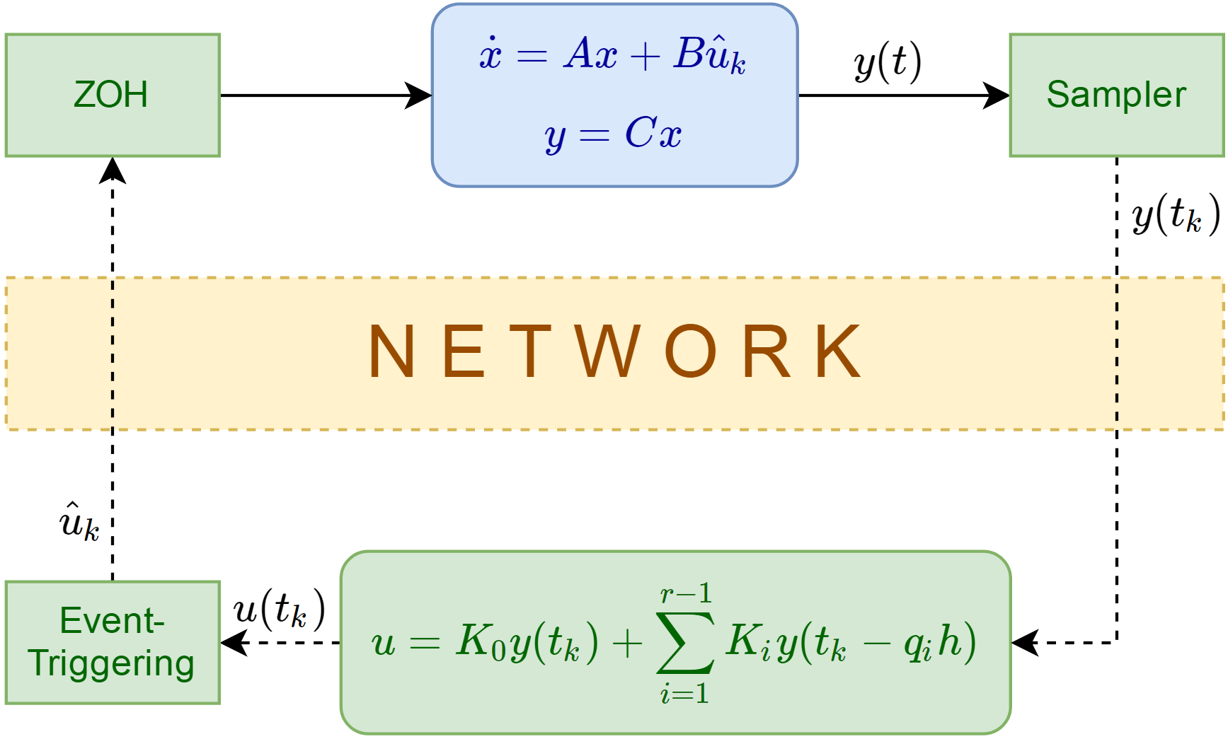
Figure 1: Event-triggering with respect to the control signal

Event-triggered control allows to reduce the number of signals transmitted through a communication network [13, 14, 15, 16, 17]. The idea is to transmit the signal only when it changes a lot. The event-triggering mechanism for measurements was implemented in [1] for the system (1), (6) with relative degree $r=2$. Here, we consider the system with $r\geq 2$ and introduce the event-triggering for control signals, since the output event-triggering leads to complicated conditions (see Remark 3).

Consider the system (Fig. 1)

$$\begin{array}[]{ll}\dot{x}(t)=Ax(t)+B\hat{u}_{k},&t\in[t_{k},t_{k+1}),\>k\in\mathbb{N}_{0},\\ y(t)=Cx(t),&x\in\mathbb{R}^{n},u\in\mathbb{R}^{m},y\in\mathbb{R}^{l},\end{array}$$ (12)

where $\hat{u}_{k}=u(t_{k})$ if $u(t_{k})$ from (6) was transmitted and $\hat{u}_{k}=\hat{u}_{k-1}$ otherwise. The signal $u(t_{k})$ is transmitted if its relative change since the last transmission is large enough, namely, if

$$(u(t_{k})-\hat{u}_{k-1})^{T}\Omega(u(t_{k})-\hat{u}_{k-1})>\sigma u^{T}(t_{k})\Omega u(t_{k}),$$ (13)

where $\sigma\in[0,1)$ and $0<\Omega\in\mathbb{R}^{m\times m}$ are event-triggering parameters. Thus, $\hat{u}_{0}=u(t_{0})$ and

$$\hat{u}_{k}=\left\{\begin{array}[]{ll}u(t_{k}),&\text{\eqref{ETC} is true,}\\ \hat{u}_{k-1},&\text{\eqref{ETC} is false.}\end{array}\right.$$ (14)

Theorem 2

Consider the system (12) subject to (2). For given sampling period $h>0$, discrete-time delays $0<q_{1}<\ldots<q_{r-1}$, controller gains $K_{0},\ldots,K_{r-1}\in\mathbb{R}^{m\times l}$, event-triggering threshold $\sigma\in[0,1)$, and decay rate $\alpha>0$, let there exist positive-definite matrices $P\in\mathbb{R}^{n\times n}$, $\Omega,W_{0},W_{i},R_{i}\in\mathbb{R}^{m\times m}$ ($i=1,\ldots,r-1$) such that $\Phi_{e}\leq 0$, where

$$\begin{array}[]{l}\Phi_{e}=\left[\begin{array}[]{cccc:cc}\lx@intercol\hfil\hbox{\multirowsetup$\Phi$}\hfil\lx@intercol&PB&\sigma([K_{0},K]M\bar{C})^{T}\Omega\\ \lx@intercol\hfil\hfil\lx@intercol&0&\sigma\mathbf{1}_{r}\otimes\Omega\\ \lx@intercol\hfil\hfil\lx@intercol&0&\sigma\mathbf{1}_{r-1}\otimes\Omega\\ \lx@intercol\hfil\hfil\lx@intercol&HCA^{r-1}\!B&0\\ \hdashline*&*&*&*&-\Omega&0\\ &*&*&*&0&-\sigma\Omega\end{array}\right]\end{array}$$

with $M$, $K$, $\bar{C}$ defined in (8) and $\Phi$, $H$ given in Theorem 1. Then the event-triggered controller (6), (13), (14) exponentially stabilizes the system (12) with the decay rate $\alpha$.

Proof is given in Appendix B.

Remark 3

The event-triggering mechanism (13), (14) is constructed with respect to the control signal. This allows to reduce the workload of a controller-to-actuator network. To compensate the event-triggering error, we add (29) to $\dot{V}$, which leads to two additional block-columns and block-rows in the LMI (confer $\Phi$ of Theorem 1 and $\Phi_{e}$ of Theorem 2). One can study the event-triggering mechanism with respect to the measurements by replacing $y(t_{k})$, $y(t_{k}-q_{i}h)$ with $\hat{y}_{k}=y(t_{k})+e_{k}$, $\hat{y}_{k-q_{i}}=y(t_{k}-q_{i}h)+e_{k-q_{i}}$ in (6). This may reduce the workload of a sensor-to-controller network but would require to add expressions similar to (29) to $\dot{V}$ for each error $e_{k},e_{k-q_{1}},\ldots,e_{k-q_{r-1}}$. This would lead to more complicated LMIs with two additional block-columns and block-rows for each error. We study the event-triggering mechanism with respect to the control for simplicity.

Remark 4

Taking $\Omega=\omega I$ with large $\omega>0$, one can show that $\Phi_{e}\leq 0$ and $\Phi\leq 0$ are equivalent for $\sigma=0$. This happens since the event-triggered control (6), (13), (14) with $\sigma=0$ degenerates into periodic sampled-data control (6). Therefore, an appropriate $\sigma$ can be found by increasing its value from zero while preserving the feasibility of the LMIs from Theorem 2.

II-C Example

Consider the triple integrator $\dddot{y}=u$, which can be presented in the form (1) with

$$A\!=\!\left[\begin{array}[]{ccc}0&1&0\\ 0&0&1\\ 0&0&0\end{array}\right],\>B=\left[\begin{array}[]{c}0\\ 0\\ 1\end{array}\right],\>C=\left[\begin{array}[]{ccc}1&0&0\end{array}\right].$$ (15)

These parameters satisfy (2) with $r=3$. The derivative-dependent control (4) with

$$\bar{K}_{0}=-2\times 10^{-4},\quad\bar{K}_{1}=-0.06,\quad\bar{K}_{2}=-0.342$$

stabilizes the system (1), (15). The LMIs of Theorem 1 are feasible for

$$\begin{array}[]{c}h=0.044,\quad q_{1}=30,\quad q_{2}=60,\quad\alpha=10^{-3},\\ K_{0}\approx-0.265,\quad K_{1}\approx 0.483,\quad K_{2}\approx-0.219,\end{array}$$

where $K_{i}$ are calculated using (11). Therefore, the delayed sampled-data controller (6) also stabilizes the system (1), (15).

Consider now the system (12), (15). The LMIs of Theorem 2 are feasible for $h=0.042$, $\sigma=2\times 10^{-3}$ with the same control gains $\bar{K}_{0}$, $\bar{K}_{1}$, $\bar{K}_{2}$, delays $q_{1}$, $q_{2}$, and decay rate $\alpha$. Thus, the event-triggered control (6), (13), (14) stabilizes the system (12), (15). Performing numerical simulations for $10$ randomly chosen initial conditions $\|x(0)\|_{\infty}\leq 1$, we find that the event-triggered control (6), (13), (14) requires to transmit on average $455.6$ control signals during $100$ seconds. The amount of transmissions for the sampled-data control (6) is given by $\lfloor\frac{100}{h}\rfloor+1=2273$. Thus, the event-triggering mechanism reduces the workload of the controller-to-actuator network by almost $80\%$ preserving the decay rate $\alpha$. Note that $\sigma>0$ leads to a smaller sampling period $h$. Therefore, the event-triggering mechanism requires to transmit more measurements through sensor-to-controller network. However, the total workload of both networks is reduced by over $37\%$.

III Event-triggered PID control

Consider the scalar system

$$\ddot{y}(t)+a_{1}\dot{y}(t)+a_{2}y(t)=bu(t)$$ (16)

and the PID controller

$$u(t)=\bar{k}_{p}y(t)+\bar{k}_{i}\int_{0}^{t}y(s)\,ds+\bar{k}_{d}\dot{y}(t).$$ (17)

Here, we study sampled-data implementation of the PID controller (17) that is obtained using the approximations

$$\begin{array}[]{l}\int_{0}^{t}y(s)\,ds\approx\int_{0}^{t_{k}}y(s)\,ds\approx h\sum_{j=0}^{k-1}y(t_{j}),\\ \dot{y}(t)\approx\dot{y}(t_{k})\approx\frac{y(t_{k})-y(t_{k-q})}{qh},\end{array}\quad t\in[t_{k},t_{k+1}),$$

where $h>0$ is a sampling period, $t_{k}=kh$, $k\in\mathbb{N}_{0}$, are sampling instants, $q\in\mathbb{N}$ is a discrete-time delay, and $y(t_{k-q})=0$ for $k<q$. Substituting these approximations into (17), we obtain the sampled-data controller

$$\begin{array}[]{r}u(t)=k_{p}y(t_{k})+k_{i}h\sum_{j=0}^{k-1}y(t_{j})+k_{d}y(t_{k-q}),\\ t\in[t_{k},t_{k+1}),\>k\in\mathbb{N}_{0},\end{array}$$ (18)

with $y(t_{k-q})=0$ for $k<q$ and

$$\textstyle k_{p}=\bar{k}_{p}+\frac{\bar{k}_{d}}{qh},\quad k_{i}=\bar{k}_{i},\quad k_{d}=-\frac{\bar{k}_{d}}{qh}.$$ (19)

Similarly to Section II-B, we introduce the event-triggering mechanism to reduce the amount of transmitted control signals. Namely, we consider the system

$$\ddot{y}(t)+a_{1}\dot{y}(t)+a_{2}y(t)=b\hat{u}_{k},\quad t\in[t_{k},t_{k+1}),\ k\in\mathbb{N}_{0},$$ (20)

where $\hat{u}_{k}$ is the event-triggered control: $\hat{u}_{0}=u(t_{0})$,

$$\hat{u}_{k}=\left\{\begin{array}[]{ll}u(t_{k}),&\text{if \eqref{ETC:PID} is true},\\ \hat{u}_{k-1},&\text{if \eqref{ETC:PID} is false},\end{array}\right.$$ (21)

with $u(t)$ from (18) and the event-triggering condition

$$(u(t_{k})-\hat{u}_{k-1})^{2}>\sigma u^{2}(t_{k}).$$ (22)

Here, $\sigma\in[0,1)$ is the event-triggering threshold.

Remark 5

We consider the event-triggering mechanism with respect to the control signal, since the event-triggering with respect to the measurements $\hat{y}_{k}=y(t_{k})+e_{k}$ leads to an accumulating error in the integral term:

$$\textstyle\int_{0}^{t_{k}}y(s)\,ds\approx h\sum_{j=0}^{k-1}\hat{y}_{j}=h\sum_{j=0}^{k-1}y(t_{j})+h\sum_{j=0}^{k-1}e_{j}.$$

III-A Stability conditions

To study the stability of (20) under the event-triggered PID control (18), (21), (22), we rewrite the closed-loop system in the state space. Let $x_{1}=y$, $x_{2}=\dot{y}$, and

$$\textstyle x_{3}(t)=(t-t_{k})y(t_{k})+h\sum_{j=0}^{k-1}y(t_{j}),\quad t\in[t_{k},t_{k+1}).$$

Introduce the errors due to sampling

$$\begin{array}[]{l}v(t)=x(t_{k})-x(t)\\ \delta(t)=y(t_{k-q})-y(t-qh),\end{array}\quad t\in[t_{k},t_{k+1}),\ k\in\mathbb{N}_{0}.$$

Using Taylor’s expansion for $y(t-qh)$ with the remainder in the integral form, we have

$$y(t_{k-q})=y(t-qh)+\delta(t)\textstyle=y(t)-\dot{y}(t)qh+\kappa(t)+\delta(t),$$

where

$$\textstyle\kappa(t)=\int_{t-qh}^{t}(s-t+qh)\ddot{y}(s)\,ds.$$

Using these representations in (18), we obtain

$$\begin{array}[]{rl}u(t_{k})&=k_{p}x_{1}(t_{k})+k_{i}x_{3}(t_{k})+k_{d}y(t_{k-q})\\ &=[k_{p}+k_{d},-qhk_{d},k_{i}]x+[k_{p},0,k_{i}]v+k_{d}(\kappa+\delta).\end{array}$$ (23)

Introduce the event-triggering error $e_{k}=\hat{u}_{k}-u(t_{k})$. Then the system (20) under the event-triggered PID control (21), (22), (23) can be presented as

$$\begin{array}[]{l}\dot{x}=Ax+A_{v}v+Bk_{d}(\kappa+\delta)+Be_{k},\\ y=Cx,\end{array}$$ (24)

for $t\in[t_{k},t_{k+1})$, $k\in\mathbb{N}_{0}$, where

$$\begin{array}[]{l}A=\begin{bmatrix}0&1&0\\ -a_{2}+b(k_{p}+k_{d})&-a_{1}-qhbk_{d}&bk_{i}\\ 1&0&0\end{bmatrix},\\ A_{v}=\begin{bmatrix}0&0&0\\ bk_{p}&0&bk_{i}\\ 1&0&0\end{bmatrix}\!,\>B=\begin{bmatrix}0\\ b\\ 0\end{bmatrix}\!,\>C=\begin{bmatrix}1&0&0\end{bmatrix}.\end{array}$$ (25)

Note that the “integral” term in (18) requires to introduce the error due to sampling $v$ that appears in (24) but was absent in (9). The analysis of $v$ is the key difference between Theorem 2 and the next result.

Theorem 3

Consider the system (20).

• For given sampling period $h>0$, discrete-time delay $q>0$, controller gains $k_{p}$, $k_{i}$, $k_{d}$, event-triggering threshold $\sigma\in[0,1)$, and decay rate $\alpha>0$, let there exist positive-definite matrices $P,S\in\mathbb{R}^{3\times 3}$ and nonnegative scalars $W$, $R$, $\omega$ such that $\Psi\leq 0$, where $\Psi=\{\Psi_{ij}\}$ is the symmetric matrix composed from

  $$\begin{array}[]{l}\Psi_{11}=PA+A^{T}P+2\alpha P+\left[\begin{smallmatrix}0&0&0\\ 0&1&0\\ 0&0&0\end{smallmatrix}\right]Wk_{d}^{2}h^{2}e^{2\alpha h},\\ \Psi_{12}=PA_{v}\sqrt{h},\quad\Psi_{13}=\Psi_{14}=\Psi_{15}=PB,\\ \Psi_{16}=\begin{bmatrix}k_{p}\!+\!k_{d}\\ -qhk_{d}\\ k_{i}\end{bmatrix}\omega\sigma,\quad\Psi_{26}=\begin{bmatrix}k_{p}\\ 0\\ k_{i}\end{bmatrix}\omega\sigma\sqrt{h},\\ \Psi_{17}=A^{T}G,\quad\Psi_{22}=-\frac{\pi^{2}}{4}Sh,\quad\Psi_{27}=A_{v}^{T}G\sqrt{h},\\ \Psi_{36}=\Psi_{46}=\omega\sigma,\quad\Psi_{37}=\Psi_{47}=\Psi_{57}=B^{T}G,\\ \Psi_{33}=-W\frac{\pi^{2}}{4}e^{-2\alpha qh},\quad\Psi_{44}=-R\frac{4}{(qh)^{2}}e^{-2\alpha qh},\\ \Psi_{55}=-\omega,\quad\Psi_{66}=-\omega\sigma,\quad\Psi_{77}=-G,\\ G=h^{2}e^{2\alpha h}S+\left[\begin{smallmatrix}0&0&0\\ 0&1&0\\ 0&0&0\end{smallmatrix}\right]Rk_{d}^{2}(qh)^{2}\end{array}$$

  with $A$, $A_{v}$, $B$, $C$ given in (25). Then, the event-triggered PID controller (18), (21), (22) exponentially stabilizes the system (20) with the decay rate $\alpha$.

• Let there exist $\bar{k}_{p}$, $\bar{k}_{i}$, $\bar{k}_{d}$ such that the PID controller (17) exponentially stabilizes the system (16) with a decay rate $\alpha^{\prime}$. Then, the event-triggered PID controller (18), (21), (22) with $k_{p}$, $k_{i}$, $k_{d}$ given by (11) and $q=\lfloor h^{-\frac{1}{2}}\rfloor$ exponentially stabilizes the system (20) with any given decay rate $\alpha<\alpha^{\prime}$ if the sampling period $h>0$ and the event-triggering threshold $\sigma\in[0,1)$ are small enough.

Proof is given in Appendix C.

Remark 6

The event-triggered control (18), (21), (22) with $\sigma=0$ degenerates into sampled-data control (18). Therefore, Theorem 3 with $\sigma=0$ gives the stability conditions for the system (16) under the sampled-data PID control (18).

Remark 7

Appropriate values of $h$ and $\sigma$ can be found in a manner similar to Remarks 2 and 4.

III-B Example

Following [8], we consider (16) with $a_{1}=8.4$, $a_{2}=0$, $b=35.71$. The system is not asymptotically stable if $u=0$. The PID controller (17) with $\bar{k}_{p}=-10$, $\bar{k}_{i}=-40$, $\bar{k}_{d}=-0.65$ exponentially stabilizes it with the decay rate $\alpha^{\prime}\approx 10.4$.

Theorem 3 with $\sigma=0$ (see Remark 6) guarantees that the sampled-data PID controller (18) can achieve any decay rate $\alpha<\alpha^{\prime}$ if the sampling period $h>0$ is small enough. Since $\alpha^{\prime}$ is on the verge of stability, $\alpha$ close to $\alpha^{\prime}$ requires to use small $h$. Thus, for $\alpha=10.3$, the LMIs of Theorem 3 are feasible with $h\approx 10^{-7}$, $q=4272$, and $k_{p}$, $k_{i}$, $k_{d}$ given by (19). To avoid small sampling period, we take $\alpha=5$.

For $\sigma=0$, $\alpha=5$ and each $q=1,2,3,\ldots$ we find the maximum sampling period $h>0$ such that the LMIs of Theorem 3 are feasible. The largest $h$ corresponds to

$$\begin{array}[]{c}\alpha=5,\quad\sigma=0,\quad q=7,\quad h=4.7\times 10^{-3},\\ k_{p}\approx-29.76,\quad k_{i}=-40,\quad k_{d}\approx 19.76,\end{array}$$

where $k_{p}$, $k_{i}$, $k_{d}$ are calculated using (19). Remark 6 implies that the sampled-data PID controller (18) stabilizes (16).

Theorem 3 remains feasible for

$$\begin{array}[]{c}\alpha=5,\quad\sigma=9\times 10^{-3},\quad q=7,\quad h=4\times 10^{-3},\\ k_{p}\approx-33.21,\quad k_{i}=-40,\quad k_{d}\approx 23.21,\end{array}$$

where $k_{p}$, $k_{i}$, $k_{d}$ are calculated using (19). Thus, the event-triggered PID control (18), (21), (22) exponentially stabilizes (20). Performing numerical simulations in a manner described in Section II-C, we find that the event-triggered PID control requires to transmit on average $628.4$ control signals during $10$ seconds. The sampled-data controller (18) requires $\left\lfloor\frac{10}{h}\right\rfloor+1=2128$ transmissions. Thus, the event-triggering mechanism reduces the workload of the controller-to-actuator network by more than $70\%$. The total workload of both networks is reduced by more than $26\%$.

Appendix A Proof of Theorem 1

(i) Consider the functional

$$V=V_{0}+V_{\delta 0}+V_{\delta}+V_{\kappa}$$ (26)

with

$$\begin{array}[]{rl}&V_{0}=x^{T}Px,\\ &V_{\delta 0}=h^{2}e^{2\alpha h}\int_{t_{k}}^{t}e^{-2\alpha(t-s)}\dot{y}^{T}(s)K_{0}^{T}W_{0}K_{0}\dot{y}(s)\,ds\\ &\phantom{V_{\delta 0}=}-\frac{\pi^{2}}{4}\int_{t_{k}}^{t}e^{-2\alpha(t-s)}[y(s)-y(t_{k})]^{T}K_{0}^{T}W_{0}\times\\ \lx@intercol\hfil K_{0}[y(s)-y(t_{k})]\,ds,\lx@intercol\\ &V_{\delta}=h^{2}e^{2\alpha h}\sum_{i=1}^{r-1}\int_{t_{k}-q_{i}h}^{t}e^{-2\alpha(t-s)}\dot{y}^{T}(s)K_{i}^{T}W_{i}K_{i}\dot{y}(s)\,ds\\ &\phantom{V_{\delta}=}-\frac{\pi^{2}}{4}\sum_{i=1}^{r-1}\int_{t_{k}-q_{i}h}^{t-q_{i}h}e^{-2\alpha(t-s)}[y(s)-y(t_{k}-q_{i}h)]^{T}\times\\ \lx@intercol\hfil K_{i}^{T}W_{i}K_{i}[y(s)-y(t_{k}-q_{i}h)]\,ds,\lx@intercol\\ &V_{\kappa}=\sum_{i=1}^{r-1}\int_{t-q_{i}h}^{t}e^{-2\alpha(t-s)}(s-t+q_{i}h)^{r}\times\\ \lx@intercol\hfil(y^{(r)}(s))^{T}K_{i}^{T}R_{i}K_{i}y^{(r)}(s)\,ds.\lx@intercol\end{array}$$

The term $V_{\kappa}$, introduced in [12], compensates Taylor’s remainders $\kappa_{i}$, while $V_{\delta 0}$ and $V_{\delta}$, introduced in [9], compensate the sampling errors $\delta_{0}$ and $\delta$. The Wirtinger inequality (Lemma 1) implies $V_{\delta 0}\geq 0$ and $V_{\delta}\geq 0$. Using (9) and (3), we obtain

$$\begin{array}[]{l}\dot{V}_{0}+2\alpha V_{0}\!=\!2x^{T}P[Dx\!+\!BK_{0}\delta_{0}\!+\!BK\delta\!+\!BK\kappa]\!+\!2\alpha x^{T}Px,\\ \dot{V}_{\delta 0}+2\alpha V_{\delta 0}=h^{2}e^{2\alpha h}x^{T}(K_{0}CA)^{T}W_{0}(K_{0}CA)x\\ \lx@intercol\hfil-\frac{\pi^{2}}{4}\delta_{0}^{T}K_{0}^{T}W_{0}K_{0}\delta_{0},\lx@intercol\\ \dot{V}_{\delta}+2\alpha V_{\delta}=h^{2}e^{2\alpha h}\sum_{i=1}^{r-1}x^{T}(K_{i}CA)^{T}W_{i}(K_{i}CA)x\\ \lx@intercol\hfil-\frac{\pi^{2}}{4}\sum_{i=1}^{r-1}e^{-2\alpha q_{i}h}\delta_{i}^{T}K_{i}^{T}W_{i}K_{i}\delta_{i}.\lx@intercol\end{array}$$

Using $y^{(r)}=CA^{r-1}\dot{x}$ (which follows from (3)) and Jensen’s inequality (Lemma 2) with $\rho(s)=(s-t+q_{i}h)^{r-1}$, we have

$$\begin{array}[]{rl}\dot{V}_{\kappa}+2\alpha V_{\kappa}=&\sum_{i=1}^{r-1}(q_{i}h)^{r}(y^{(r)}(t))^{T}K_{i}^{T}R_{i}K_{i}y^{(r)}(t)\\ \textstyle\hfil&-\sum_{i=1}^{r-1}r\int_{t-q_{i}h}^{t}e^{-2\alpha(t-s)}(s-t+q_{i}h)^{r-1}\times\\ &\lx@intercol\hfil(y^{(r)}(s))^{T}K_{i}^{T}R_{i}K_{i}y^{(r)}(s)\,ds\lx@intercol\\ \leq&\sum_{i=1}^{r-1}(q_{i}h)^{r}\dot{x}^{T}(A^{r-1})^{T}C^{T}K_{i}^{T}R_{i}K_{i}CA^{r-1}\dot{x}\\ &\lx@intercol\hfil-\sum_{i=1}^{r-1}\frac{(r!)^{2}}{(q_{i}h)^{r}}e^{-2\alpha q_{i}h}\kappa_{i}^{T}K_{i}^{T}R_{i}K_{i}\kappa_{i}.\lx@intercol\end{array}$$

Summing up, we obtain

$$\dot{V}+2\alpha V\leq\varphi^{T}\bar{\Phi}\varphi+\dot{x}^{T}(CA^{r-1})^{T}H(CA^{r-1})\dot{x},$$ (27)

where

$$\varphi=\operatorname{col}\{x,K_{0}\delta_{0},\ldots,K_{r-1}\delta_{r-1},K_{1}\kappa_{1},\ldots,K_{r-1}\kappa_{r-1}\}$$ (28)

and $\bar{\Phi}$ is obtained from $\Phi$ by removing the last block-column and block-row. Substituting (9) for $\dot{x}$ and applying the Schur complement, we find that $\Phi\leq 0$ guarantees $\dot{V}\leq-2\alpha V$. Since $V(t_{k})\leq V(t_{k}^{-})$, the latter implies exponential stability of the system (9) and, therefore, (1), (6).

(ii) Since $q_{i}=O(h^{\frac{1}{r}-1})$, [12, Lemma 2.1] guaranties $M^{-1}=O(h^{\frac{1}{r}-1})$, which implies $K_{i}=O(h^{\frac{1}{r}-1})$ for $i=0,\ldots,r-1$. Since $D=\bar{D}$ (with $\bar{D}$ defined in (10)) and (1), (4) is exponentially stable with the decay rate $\alpha^{\prime}$, there exists $P>0$ such that $PD+D^{T}P+2\alpha P<0$ for any $\alpha<\alpha^{\prime}$. Choose $W_{0}=O(h^{-\frac{1}{r}})$, $W_{i}=O(h^{-\frac{1}{r}})$, and $R_{i}=O(h^{1-\frac{1}{r}})$ for $i=1,\ldots,r-1$. Applying the Schur complement to $\Phi\leq 0$, we obtain

$$PD+D^{T}P+2\alpha P+O(h^{\frac{1}{r}})<0,$$

which holds for small $h>0$. Thus, (i) guarantees (ii).

Appendix B Proof of Theorem 2

Denote $e_{k}=\hat{u}_{k}-u(t_{k})$, $k\in\mathbb{N}_{0}$. The event-triggering mechanism (13), (14) guarantees

$$0\leq\sigma u^{T}(t_{k})\Omega u(t_{k})-e_{k}^{T}\Omega e_{k}.$$ (29)

Substituting $\hat{u}_{k}=u(t_{k})+e_{k}$ into (12) and using (7), we obtain (cf. (9))

$$\dot{x}=Dx+BK_{0}\delta_{0}+BK\delta+BK\kappa+Be_{k},\quad t\in[t_{k},t_{k+1})$$ (30)

with $D$ given in (9). Consider $V$ from (26). Calculations similar to those from the proof of Theorem 1 lead to (cf. (27))

$$\begin{array}[]{l}\dot{V}+2\alpha V\stackrel{{\scriptstyle\eqref{Sproc}}}{{\leq}}\dot{V}+2\alpha V+\sigma u^{T}(t_{k})\Omega u(t_{k})-e_{k}^{T}\Omega e_{k}\\ \leq\varphi_{e}^{T}\bar{\Phi}_{e}\varphi_{e}+\dot{x}^{T}(CA^{r-1})^{T}H(CA^{r-1})\dot{x}+\sigma u^{T}(t_{k})\Omega u(t_{k}),\end{array}$$

where $\varphi_{e}=\operatorname{col}\{\varphi,e_{k}\}$ (with $\varphi$ from (28)) and $\bar{\Phi}_{e}$ is obtained from $\Phi_{e}$ by removing the blocks $\Phi_{ij}$ with $i\in\{4,6\}$ or $j\in\{4,6\}$. Substituting (30) for $\dot{x}$ and (7) for $u(t_{k})$ and applying the Schur complement, we find that $\Phi_{e}\leq 0$ guarantees $\dot{V}\leq-2\alpha V$. Since $V(t_{k})\leq V(t_{k}^{-})$, the latter implies exponential stability of the system (30) and, therefore, (12) under the controller (6), (13), (14).

Appendix C Proof of Theorem 3

(i) Consider the functional

$$V=V_{0}+V_{v}+V_{\delta}+V_{\kappa}$$

with

$$\begin{array}[]{rl}V_{0}=&x^{T}Px,\\ V_{v}=&h^{2}e^{2\alpha h}\int_{t_{k}}^{t}e^{-2\alpha(t-s)}\dot{x}^{T}(s)S\dot{x}(s)\,ds\\ \lx@intercol\hfil-\frac{\pi^{2}}{4}\int_{t_{k}}^{t}e^{-2\alpha(t-s)}v^{T}(s)Sv(s)\,ds,\lx@intercol\\ V_{\delta}=&Wk_{d}^{2}h^{2}e^{2\alpha h}\int_{t_{k}-qh}^{t}e^{-2\alpha(t-s)}(\dot{y}(s))^{2}\,ds\\ &-Wk_{d}^{2}\frac{\pi^{2}}{4}\int_{t_{k}-qh}^{t-qh}e^{-2\alpha(t-s)}[y(s)-y(t_{k}-qh)]^{2}ds,\\ V_{\kappa}=&Rk_{d}^{2}\int_{t-qh}^{t}e^{-2\alpha(t-s)}(s-t+qh)^{2}(\ddot{y}(s))^{2}\,ds.\\ \end{array}$$

The Wirtinger inequality (Lemma 1) implies $V_{v}\geq 0$ and $V_{\delta}\geq 0$. Using the representation (24), we obtain

$$\begin{array}[]{l}\dot{V}_{0}+2\alpha V_{0}=2x^{T}P[Ax(t)+A_{v}v(t)+Bk_{d}(\kappa+\delta)+Be_{k}]\\ \lx@intercol\hfil+2\alpha x^{T}Px,\lx@intercol\\ \dot{V}_{v}+2\alpha V_{v}=h^{2}e^{2\alpha h}\dot{x}^{T}(t)S\dot{x}(t)-\frac{\pi^{2}}{4}v^{T}(t)Sv(t),\\ \dot{V}_{\delta}+2\alpha V_{\delta}=Wk_{d}^{2}h^{2}e^{2\alpha h}(x_{2}(t))^{2}-Wk_{d}^{2}\frac{\pi^{2}}{4}e^{-2\alpha qh}\delta^{2}(t).\end{array}$$

Using Jensen’s inequality (Lemma 2) with $\rho(s)=(s-t+q_{i}h)$, we obtain

$$\begin{array}[]{rl}\dot{V}_{\kappa}+2\alpha V_{\kappa}=&Rk_{d}^{2}(qh)^{2}(\ddot{y}(t))^{2}\\ &-Rk_{d}^{2}2\int_{t-qh}^{t}e^{-2\alpha(t-s)}(s-t+qh)(\ddot{y}(s))^{2}\,ds\\ \leq&Rk_{d}^{2}(qh)^{2}(\dot{x}_{2}(t))^{2}-Rk_{d}^{2}\frac{4}{(qh)^{2}}e^{-2\alpha qh}\kappa^{2}(t).\end{array}$$

For $\omega\geq 0$, the event-triggering rule (21), (22) guarantees

$$0\leq\omega\sigma u^{2}(t_{k})-\omega e_{k}^{2}.$$

Thus, we have

$$\textstyle\dot{V}+2\alpha V\leq\dot{V}+2\alpha V+[\omega\sigma u^{2}(t_{k})-\omega e_{k}^{2}]\\ \textstyle\leq\psi^{T}\bar{\Psi}\psi+\dot{x}^{T}(t)G\dot{x}(t)+\omega\sigma u^{2}(t_{k}),$$

where $\psi=\operatorname{col}\{x,v/\sqrt{h},k_{d}\delta,k_{d}\kappa,e_{k}\}$ and $\bar{\Psi}$ is obtained from $\Psi$ by removing the last two block-columns and block-rows. Substituting (24) for $\dot{x}$ and (23) for $u(t_{k})$ and applying the Schur complement, we find that $\Psi\leq 0$ guarantees $\dot{V}\leq-2\alpha V$. Since $V(t_{k})\leq V(t_{k}^{-})$, the latter implies exponential stability of the system (24) and, therefore, (18), (20)–(22).

(ii) The closed-loop system (16), (17) is equivalent to $\dot{x}=\bar{A}x$ with

$$\bar{A}=\begin{bmatrix}0&1&0\\ -a_{2}+b\bar{k}_{p}&-a_{1}+b\bar{k}_{d}&b\bar{k}_{i}\\ 1&0&0\end{bmatrix},\quad x=\begin{bmatrix}y\\ \dot{y}\\ \int_{0}^{t}y(s)\,ds\end{bmatrix}.$$

Since $q=O(\frac{1}{\sqrt{h}})$, relations (19) imply $k_{p}=O(\frac{1}{\sqrt{h}})$, $k_{d}=O(\frac{1}{\sqrt{h}})$. Since (16), (17) is exponentially stable with the decay rate $\alpha^{\prime}$ and (19) implies $A=\bar{A}$, there exists $P>0$ such that $PA+A^{T}P+2\alpha P<0$ for any $\alpha<\alpha^{\prime}$. Choose $S=O(\frac{1}{h\sqrt{h}})$, $W=O(\frac{1}{\sqrt{h}})$, $R=O(\sqrt{h})$, and $\omega=O(\frac{1}{\sqrt{h}})$. Applying the Schur complement to $\Psi\leq 0$, we obtain

$$PA+A^{T}P+2\alpha P+O(\sqrt{h})+\sigma F<0$$

with some $F$ independent of $\sigma$. The latter holds for small $h>0$ and $\sigma\geq 0$. Thus, (i) guarantees (ii).

References

• [1] A. Selivanov and E. Fridman, “Simple conditions for sampled-data stabilization by using artificial delay,” in 20th IFAC World Congress, 2017, pp. 13 837–13 841.
• [2] A. Ilchmann and C. J. Sangwin, “Output feedback stabilisation of minimum phase systems by delays,” Systems & Control Letters, vol. 52, no. 3-4, pp. 233–245, 2004.
• [3] S. I. Niculescu and W. Michiels, “Stabilizing a chain of integrators using multiple delays,” IEEE Transactions on Automatic Control, vol. 49, no. 5, pp. 802–807, 2004.
• [4] I. Karafyllis, “Robust global stabilization by means of discrete-delay output feedback,” Systems & Control Letters, vol. 57, no. 12, pp. 987–995, 2008.
• [5] A. Ramírez, R. Sipahi, S. Mondié, and R. R. Garrido, “An Analytical Approach to Tuning of Delay-Based Controllers for LTI-SISO Systems,” SIAM Journal on Control and Optimization, vol. 55, no. 1, pp. 397–412, 2017.
• [6] M. French, A. Ilchmann, and M. Mueller, “Robust stabilization by linear output delay feedback,” SIAM Journal on Control and Optimization, vol. 48, no. 4, pp. 2533–2561, 2009.
• [7] Y. Okuyama, “Discretized PID Control and Robust Stabilization for Continuous Plants,” in IFAC Proceedings Volumes, vol. 41, no. 2, 2008, pp. 14 192–14 198.
• [8] A. Ramírez, S. Mondié, R. Garrido, and R. Sipahi, “Design of Proportional-Integral-Retarded (PIR) Controllers for Second-Order LTI Systems,” IEEE Transactions on Automatic Control, vol. 61, no. 6, pp. 1688–1693, 2016.
• [9] K. Liu and E. Fridman, “Wirtinger’s inequality and Lyapunov-based sampled-data stabilization,” Automatica, vol. 48, no. 1, pp. 102–108, 2012.
• [10] A. Seuret and C. Briat, “Stability analysis of uncertain sampled-data systems with incremental delay using looped-functionals,” Automatica, vol. 55, pp. 274–278, 2015.
• [11] E. Fridman and L. Shaikhet, “Delay-induced stability of vector second-order systems via simple Lyapunov functionals,” Automatica, vol. 74, pp. 288–296, 2016.
• [12] ——, “Stabilization by using artificial delays: An LMI approach,” Automatica, vol. 81, pp. 429–437, 2017.
• [13] K. J. Åström and B. Bernhardsson, “Comparison of Periodic and Event Based Sampling for First-Order Stochastic Systems,” in 14th IFAC World Congress, 1999, pp. 301–306.
• [14] P. Tabuada, “Event-Triggered Real-Time Scheduling of Stabilizing Control Tasks,” IEEE Transactions on Automatic Control, vol. 52, no. 9, pp. 1680–1685, 2007.
• [15] W. P. M. H. Heemels, K. H. Johansson, and P. Tabuada, “An introduction to event-triggered and self-triggered control,” in IEEE Conference on Decision and Control, 2012, pp. 3270–3285.
• [16] W. P. M. H. Heemels, M. C. F. Donkers, and A. R. Teel, “Periodic Event-Triggered Control for Linear Systems,” IEEE Transactions on Automatic Control, vol. 58, no. 4, pp. 847–861, 2013.
• [17] A. Selivanov and E. Fridman, “Event-Triggered $H_{\infty}$ Control: A Switching Approach,” IEEE Transactions on Automatic Control, vol. 61, no. 10, pp. 3221–3226, 2016.
• [18] ——, “Observer-based input-to-state stabilization of networked control systems with large uncertain delays,” Automatica, vol. 74, pp. 63–70, 2016.
• [19] O. Solomon and E. Fridman, “New stability conditions for systems with distributed delays,” Automatica, vol. 49, no. 11, pp. 3467–3475, 2013.