Action of Clifford algebra on the space of sequences of transfer operators

Abstract.

We deduce from a determinant identity on quantum transfer matrices of generalized quantum integrable spin chain model their generating functions. We construct the isomorphism of Clifford algebra modules of sequences of transfer matrices and the boson space of symmetric functions. As an application, tau-functions of transfer matrices immediately arise from classical tau-functions of symmetric functions.

1. Introduction

Connections between transfer matrices of quantum integrable models and solutions of classical integrable hierarchies of non-linear partial differential equations, observed in [12], were developed later in a series of papers [1], [2], [18], [19], etc. The authors of [1] defined a generating function of commuting quantum transfer matrices of a generalized quantum integrable spin chain. They proved that this master $T$-operator obeys Hirota bilinear equations (see e.g. [5], [6], [15]), identifying it with a tau-function of the KP hierarchy. In [2], [18], [19] similar identification is obtained for the quantum inhomogeneous XXX spin chain of $GL(N)$ type with twisted boundary conditions, quantum spin chain with trigonometric $R$-matrix, and the quantum Gaudin model with twisted boundary conditions.

In this note we consider another generating function for quantum transfer matrices of a generalized quantum integrable spin chain. We describe combinatorial properties of this generating function and define the action of Clifford algebra on a space spanned by sequences of quantum transfer matrices. This approach suggests another interpretation of the connections of transfer matrices to $\tau$-function formalism, the one that refers to the construction of the classical Hirota bilinear equations from the vertex operator action of Clifford algebra on the boson space of symmetric functions. One can mention that the master $T$-operator of [1] generalizes the right-hand side of the Cauchy-Littlewood identity

$$\prod_{ij}(1-a_{i}x_{j})^{-1}=\sum_{\lambda}s_{\lambda}({a})s_{\lambda}({x}),$$

where $s_{\lambda}({a})$, $s_{\lambda}({x})$ are symmetric Schur functions in two independent sets of variables $a=(a_{1},a_{2},\dots)$ and $x=(x_{1},x_{2},\dots)$ (see e.g. [14], I.4 (4.3)), while the generating function in this note is the analogue of the generating function for Schur functions of the form

$$\prod_{i<j}\left(1-\frac{x_{j}}{x_{i}}\right)\prod_{i=1}^{l}H(x_{i})=\sum_{l(\lambda)\leq l}s_{\lambda}({a})x_{1}^{\lambda_{1}}\cdots x_{l}^{\lambda_{l}},$$ (1.1)

where $H(x)=\sum_{k}h_{k}({a})x^{k}$ is the generating function for complete symmetric functions $h_{k}({a})$ (see e.g. [14], I.5, Example 29 (7)).

In Section 2 we introduce the necessary notations and definitions, and describe the properties of generating functions of transfer matrix. In Section 3 we construct the action of Clifford algebra on the space of sequences of $T$-operators. In Section 4 we make some remarks on bosonisation of the action of Clifford algebra.

2. Properties of Transfer operators

2.1. Notations and definitions

Let $\{e_{ij}\}_{i,j=1,\dots,N}$ be the set of standard generators of the universal enveloping algebra $U(\mathfrak{gl}_{N}({\mathbb{C}}))$. The action of these generators on ${\mathbb{C}}^{N}$ is given by the elementary matrices $\{E_{ij}\}_{i,j=1,\dots,N}$. Let partition $\lambda=(\lambda_{1}\geq\dots\geq\lambda_{l}>0)$ with $\lambda_{i}\in{\mathbb{Z}}_{\geq 0}$ and the length $l\leq N$ be the highest weight of an irreducible finite-dimensional $U(\mathfrak{gl}_{N}({\mathbb{C}}))$-representation $\pi_{\lambda}$ acting on the space $V_{\lambda}$. We will use the same notation for the corresponding representation of $GL_{N}({\mathbb{C}})$. Consider $R$-matrix given by a linear function in variable $u$ with coefficients in $\operatorname{End}\,V_{\lambda}\otimes\operatorname{End}\,{\mathbb{C}}^{N}$:

$$R(u)=1+\frac{1}{u}\sum_{ij}\pi_{\lambda}(e_{ji})\otimes E_{ij}.$$ (2.1)

Let $R_{0i}(u)$ be the operator that acts as $R$-matrix (2.1) on the $0$-th component $V_{\lambda}$ and on the $i$-th component ${\mathbb{C}}^{N}$ of the tensor product $V_{\lambda}\otimes({\mathbb{C}}^{N})^{\otimes n}$. We fix a collection of complex parameters $a=(a_{i})_{i=1,2,\dots}$. Let $g$ be an invertible $N$ by $N$ matrix, called the twist matrix, with eigenvalues $(g_{1},\dots,g_{N})$. Consider a family of quantum transfer matrices ($T$-operators) $T_{\lambda}(u)=T_{\lambda,n}^{N}(u,a)(g)$ defined by

$$T_{\lambda,n}^{N}(u,a)(g)=\begin{cases}tr_{V_{\lambda}}\left(R_{01}(u-a_{1})\dots R_{0n}(u-a_{n})(\pi_{\lambda}(g)\otimes Id^{\otimes n})\right),&\text{if}\quad l\leq N,\\ 0,&\text{if}\quad l>N,\end{cases}$$ (2.2)

where the trace is taken over the $0$-th component $V_{\lambda}$. We think of these $T$-operators as functions from $GL_{N}({\mathbb{C}})$ to the space of $\text{Hom}(({\mathbb{C}}^{N})^{\otimes n})[1/u]$. We will omit $n,g,a$ and $N$ labels and write $T_{\lambda}(u)$ or $T^{N}_{\lambda}(u)$ when no confusion arrises.

The R-matirx (2.1) is an image of the universal $R$-matrix of the Yangian $Y(\mathfrak{gl}_{N}({\mathbb{C}}))$, and the quantum Yang-Baxter equation on the universal $R$-matrix implies that $T$-operators (2.2) commute for a fixed twist matrix $g$, a fixed collection of parameters $a=(a_{i})_{i=1,2,\dots}$ and for all $u$ and $\lambda$.

Remark 2.1.

When $n=0$, the element $T_{\lambda}(u)=tr\,{\pi_{\lambda}(g)}$ coincides with the value of the character of $\pi_{\lambda}$ on $g$ given by Schur polynomial $s_{\lambda}(g_{1},\dots,g_{N})$ of the eigenvalues of the matrix $g$. Also $T_{\lambda}(u)\to s_{\lambda}(g_{1},\dots,g_{N})\,Id^{\otimes n}$ when $u\to\infty$.

2.2. CBR determinant

Introduce the notation $h_{k}(u)=T_{(k)}(u)$ for $k=1,2,\dots$. It is also convenient to set $h_{k}(u)=0$ for $k=-1,-2,\dots$, and $h_{0}(u)=1$. Then the the following remarkable relation between $T$-matrices was observed in [3], [4] (see also [13]).

Theorem 2.1 (Cherednik-Bazhanov-Reshetikhin (CBR) determinant).

$$T_{\lambda}(u)=\det_{i,j=1,\dots,l}h_{\lambda_{i}-i+j}(u-j+1).$$ (2.3)

This formula is an analogue of Jacobi – Trudi identity for Schur symmetric functions. It not only implies several important properties of transfer matrices $T_{\lambda}(u)$, but leads to the action of Clifford algebra of fermions on the linear space spanned by sequences of $T$-matrices. For the later goal we follow the approach developed in [8], [9].

2.3. Newton’s identity

For any $u$ set $e_{k}(u)=T_{(1^{k})}(u)$ for $k=1,2\dots$, and $e_{k}(u)=0$ for $k=-1,-2$, as well as $e_{0}(u)=1$. Then from (2.3) for $k=1,2,\dots$,

$$e_{k}(u)=T_{(1)^{k}}(u)=\det_{i,j=1,\dots,k}[h_{1-i+j}(u-j+1)].$$ (2.4)

Proposition 2.1.

a) The following analogue of Newton’s formula relation holds:

$$\sum_{p=-\infty}^{+\infty}(-1)^{a-p}h_{b+p}(u-p)e_{-p-a}(u-p-1)=\delta_{a,b}\quad\text{for any $a,b\in{\mathbb{Z}}$.}$$ (2.5)

b) Let $\lambda^{\prime}=(\lambda^{\prime}_{1},\dots,\lambda^{\prime}_{k})$ be the conjugate partition of the partition $\lambda$. Then the dual (equivalent) form of (2.3) holds:

$$T_{\lambda}(u)=\det_{i,j=1,\dots,k}[e_{\lambda^{\prime}_{i}-i+j}(u+j-1)].$$ (2.6)

Proof.

Relation (2.5) follows from the recursive expansion of the determinant (2.4) for $e_{b-a}(u+b-1)$ by the first row. Then (2.5) implies that the upper triangular infinite matrices

$$\mathcal{H}=(\,h_{p-b}(u-p)\,)_{b,p\,\in{\mathbb{Z}}},\quad\mathcal{E}=(\,(-1)^{a-p}e_{a-p}(u-p-1)\,)_{p,a\,\in{\mathbb{Z}}}$$

satisfy the identity $\mathcal{H}\mathcal{E}=Id$, and (2.6) follows from the standard argument on the relations on minors of matrices that are inverse of each other (see e.g. Lemma A.42 of [7]). ∎

Remark 2.2.

For some applications it is convenient to write Newton’s formula in the form of an equation on generating functions:

$$YH(u|t)YE(u-1|t)=1,$$

where

$$YH(u|t)=\sum_{s=0}^{\infty}(te^{-\partial_{u}})^{s}h_{s}(u),\quad YE(u|t)=\sum_{s=0}^{\infty}(-1)^{s}e_{s}(u)(te^{-\partial_{u}})^{s}$$

are generating functions for operators acting on the space of $\text{Hom}\,({\mathbb{C}}^{N})^{\otimes n}$-valued functions in variable $u$, and $e^{\partial_{u}}(f(u))=f(u+1)$ is the a shift operator of the variable $u$. Indeed,

$$YH(u|t)YE(u-1|t)=\sum_{s,p\,=0}^{\infty}h_{s}(u-s)(-1)^{p}e_{p}(u-s-1)(te^{-\partial_{u}})^{s+p}$$

$$=\sum_{m}\left(\sum_{s=0}^{\infty}h_{s}(u-s)(-1)^{m-s}e_{m-s}(u-s-1)\right)(te^{-\partial_{u}})^{m}=1.$$

Remark 2.3.

From definition (2.2), it follows that infinite matrix $\mathcal{E}$ and infinite formal series $YE(u|t)$ contain only finite number of non-zero terms $e_{k}(u)=e^{N}_{k,n}(u,a)(g)$.

Remark 2.4.

In [16] common eigenvalues and common eigenvectors of higher transfer matrices of an XXX-type model are studied through a certain generating function of transfer matrices with coefficients in the Yangian $Y(\mathfrak{gl}_{N}({\mathbb{C}}))$ (see formula (4.16) in [16]), and earlier in [17], the higher transfer matrices of the Gaudin model were constructed explicitly as a limit of that generating function. Up to a multiplication by a rational function of $u$, the generating function $YE(u|t)$ is the image of the generating function considered in [16], [17] under the evaluation representation ${\mathbb{C}}_{N}(a_{1})\otimes\dots\otimes{\mathbb{C}}_{N}(a_{n})$ of $Y(\mathfrak{gl}_{N}({\mathbb{C}}))$.

2.4. Transfer matrices labeled by integer vectors

Formula (2.3) allows us to extend the notion of $T_{\alpha}(u)$ for any integer vector $\alpha=(\alpha_{1},\dots,\alpha_{l})$, $\alpha_{i}\in{\mathbb{Z}}$, by literally setting

$$T_{\alpha}(u)=\det[h_{\alpha_{i}-i+j}(u-j+1)].$$ (2.7)

Note that

$$T_{(\dots,\alpha_{i},\alpha_{i+1},\dots)}(u)=-T_{(\dots,\,\alpha_{i+1}-1\,,\,\alpha_{i}+1\,,\dots)}(u),$$ (2.8)

and that $T_{\alpha}(u)=0$ whenever $\alpha_{i}-i=\alpha_{j}-j$ for some $i,j$.

Similarly, we can use formula (2.6) to extend the definition of transfer matrices to integer vectors. Set

$$T_{\alpha^{\prime}}(u)=\det_{i,j=1,\dots,k}[e_{\alpha_{i}-i+j}(u+j-1)].$$ (2.9)

While we do not define here the conjugation on arbitrary integer vector, the notation $T_{\alpha^{\prime}}(u)$ for the expression (2.9) is justified by the following lemma.

Lemma 2.1.

Let $\alpha=(\alpha_{1},\dots,\alpha_{l})$ be an integer vector, let $\rho=\rho_{l}=(0,1,\dots,l-1)$. Let $T_{\alpha}(u)$ and $T_{\alpha^{\prime}}(u)$ be defined by (2.7), (2.9). Then

$$T_{\alpha}(u)=\begin{cases}(-1)^{\sigma}T_{\lambda}(u),&\quad\text{if}\quad\alpha-\rho=\sigma(\lambda-\rho)\,\text{for some partition}\,\lambda\,\text{and}\,\sigma\in S_{l},\\ 0,&\text{otherwise.}\end{cases}$$ (2.10)

$$T_{\alpha^{\prime}}(u)=\begin{cases}(-1)^{\sigma}T_{\lambda^{\prime}}(u),&\quad\text{if}\quad\alpha-\rho=\sigma(\lambda-\rho)\,\text{for some partition}\,\lambda\,\text{and}\,\sigma\in S_{l},\\ 0,&\text{otherwise.}\end{cases}$$ (2.11)

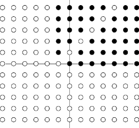
Figure 1. Non-zero values of $T_{(\alpha_{1},\alpha_{2})}(u)$ for $N\geq 2$.

Figure 1 illustrates the distribution of non-zero values of $T$-operators for integer vectors $(\alpha_{1},\alpha_{2})$ for $N\geq 2$. Black points represent integer vectors $(\alpha_{1},\alpha_{2})$ with non-vanishing transfer matrices $T_{(\alpha_{1},\alpha_{2})}(u)$.

2.5. Generating functions of $T$-operators

Set

$$H^{N}(x|u)=\sum_{k=0}^{\infty}h^{N}_{k}(u)x^{k},\quad E^{N}(x|u)=\sum_{k=0}^{\infty}(-1)^{k}e^{N}_{k}(u)x^{k}.$$

Proposition 2.2.

For any integer vector $\alpha$, the transfer matrix $T^{N}_{\alpha}(u)$ is the coefficient of $x_{1}^{\alpha_{1}}\dots x_{l}^{\alpha_{l}-l+1}$ in

$$H^{N}(x_{1},\dots,x_{l}|u) =\det\left[{x_{i}^{-j+1}}H^{N}(x_{i}|u-j+1)\right]$$ (2.12)

$$=\left.\left(\prod_{1\leq i<j\leq l}\left(\frac{e^{-\partial_{u_{j}}}}{x_{j}}-\frac{e^{-\partial_{u_{i}}}}{x_{i}}\right)\prod_{i=1}^{l}H^{N}(x_{i}|u_{i})\right)\right|_{u_{1}=u_{2}=\dots=u_{l}=u}.$$

Similarly, $(-1)^{A}T^{N}_{\alpha^{\prime}}(u)$ with $A=\sum(\alpha_{i}-i+1)$ is the coefficient of $x_{1}^{\alpha_{1}}\dots x_{l}^{\alpha_{l}-l+1}$ in

$$E^{N}(x_{1},\dots,x_{l}|u) =\det\left[{(-x_{i})^{-j+1}}E^{N}(x_{i}|u+j-1)\right]$$ (2.13)

$$=\left.\left(\prod_{1\leq i<j\leq l}\left(\frac{e^{\partial_{u_{i}}}}{x_{i}}-\frac{e^{\partial_{u_{j}}}}{x_{j}}\right)\prod_{i=1}^{l}E^{N}(x_{i}|u_{i})\right)\right|_{u_{1}=u_{2}=\dots=u_{l}}.$$

Proof.

The first statement of (2.12) follows from the expansion of the determinant as a sum over permutations:

$$\sum_{\alpha\in{\mathbb{Z}}^{l}}T^{N}_{\alpha}(u)x_{1}^{\alpha_{1}}\dots x_{l}^{\alpha_{l}-l+1}=\sum_{\alpha\in{\mathbb{Z}}^{l}}\det[h^{N}_{\alpha_{i}-i+j}(u-j+1)]x_{1}^{\alpha_{1}}\dots x_{l}^{\alpha_{l}-l+1}$$

$$=\sum_{\alpha\in{\mathbb{Z}}^{l}}\sum_{\sigma\in S_{l}}(-1)^{\sigma}h^{N}_{\alpha_{1}-1+\sigma(1)}(u-\sigma(1)+1)\dots h^{N}_{\alpha_{l}-l+\sigma(l)}(u-\sigma(l)+1)x_{1}^{\alpha_{1}}\dots x_{l}^{\alpha_{l}-l+1}$$

$$=\sum_{\sigma\in S_{l}}\sum_{(a_{1},\dots,a_{l})\in{\mathbb{Z}}^{l}}(-1)^{\sigma}h^{N}_{a_{1}}(u-\sigma(1)+1)\dots h^{N}_{a_{l}}(u-\sigma(l)+1)x_{1}^{a_{1}-\sigma(1)+1}\dots x_{l}^{a_{l}-\sigma(l)+1}$$

$$=\sum_{\sigma\in S_{l}}(-1)^{\sigma}H^{N}(x_{1}|u-\sigma(1)+1)\dots H^{N}(x_{l}|u-\sigma(l)+1)x_{1}^{-\sigma(1)+1}\dots x_{l}^{-\sigma(l)+1}$$

$$=\det\left[{x_{i}^{-j+1}}H^{N}(x_{i}|u-j+1)\right].$$

For the second part of (2.12), which can be viewed as a generalization of (1.1), consider a set of independent variables $(u_{1},\dots,u_{l})$. Define

$$H^{N}(x_{1},\dots,x_{l}|u_{1},\dots,u_{l})=\det\left[{x_{i}^{-j+1}}H^{N}(x_{i}|u_{i}-j+1)\right].$$

Then

$$H^{N}(x_{1},\dots,x_{l}|u_{1},\dots u_{l})=\sum_{\sigma\in S_{l}}(-1)^{\sigma}\left({x_{1}}{e^{\partial_{u_{1}}}}\right)^{1-\sigma(1)}H^{N}(x_{1}|u_{1})\dots\left({x_{l}}e^{\partial_{u_{l}}}\right)^{1-\sigma(l)}H^{N}(x_{1}|u_{1})$$

$$=\det[(x_{i}e^{\partial_{u_{i}}})^{1-j}]\prod_{i=1}^{l}H^{N}(x_{i}|u_{i})=\prod_{1\leq i<j\leq l}\left(\frac{e^{-\partial_{u_{j}}}}{x_{j}}-\frac{e^{-\partial_{u_{i}}}}{x_{i}}\right)\prod_{i=1}^{l}H^{N}(x_{i}|u_{i}),$$

and the second statement follows. The proof of (2.13) is exactly the same. ∎

3. Clifford algebra action on the space of sequences of transfer matrices

3.1. Clifford algebra action on symmetric functions

Our next goal is to define the action of Clifford algebra on a space generated by transfer matrices, which will allow us to establish connections to the classical boson-fermion correspondence and $\tau$-function formalism. Clifford algebra $Cl$ is generated by elements $\{\psi^{\pm}_{k}\}_{k\in{\mathbb{Z}}}$ with the relations

$$\psi^{+}_{k}\psi^{-}_{l}+\psi^{-}_{l}\psi^{+}_{k}=\delta_{k,l},\quad\psi^{\pm}_{k}\psi^{\pm}_{l}+\psi^{\pm}_{l}\psi^{\pm}_{k}=0.$$ (3.1)

This infinite Clifford algebra originates from the vector space $W=(\oplus_{i}{\mathbb{C}}\psi^{+}_{i})\bigoplus(\oplus_{i}{\mathbb{C}}\psi^{-}_{i})$ with the bilinear form that is defined by $(\psi^{+}_{i},\psi^{-}_{j})=\delta_{ij}$, and the rest of the values being zeros.

The crucial component of the classical boson-fermion correspondence refers to the action of $Cl$ on the space of symmetric functions, which we reproduce here in purely combinatorial terms. Let $z$ be a formal variable and let $\mathcal{B}^{(m)}$ be the linear span of the set of basis vectors $\{z^{m}s_{\lambda}\}$, where $s_{\lambda}$ are Schur symmetric functions taken over all partitions $\lambda$. Note that each $\mathcal{B}^{(m)}$ is just a copy of the ring of symmetric functions. Set

$$\mathcal{B}=\oplus_{m\in{\mathbb{Z}}}\mathcal{B}^{(m)}.$$

The action of operators $\psi^{\pm}_{k}$ on $\{z^{m}s_{\lambda}\}$ is given by the following rules:

$$\psi^{+}_{k}(z^{m}s_{\lambda}) =z^{m+1}s_{(k-m-1,\lambda)},$$ (3.2)

$$\psi^{-}_{k}(z^{m}s_{\lambda}) =z^{m-1}\sum_{t=1}^{\infty}(-1)^{t+1}\delta_{k-m-1,\,\lambda_{t}-t}\,s_{(\lambda_{1}+1,\dots,\lambda_{t-1}+1,\lambda_{t+1},\lambda_{t+2}\dots)},$$ (3.3)

where again for any integer vector $\alpha$ of $l$ parts, one sets $s_{\alpha}=(-1)^{\sigma}s_{\lambda}$, if $\alpha-\rho=\sigma(\lambda-\rho)$ for some partition $\lambda$ and some permutation $\sigma$, and $s_{\alpha}=0$ otherwise. Note that only one term survives in the sum (3.3). One of the easiest ways to check that operators $\psi^{\pm}_{k}$ satisfy the relations of Clifford algebra is through identification of basis elements $z^{m}s_{\lambda}$ with semi-infinite monomials of fermionic Fock space

$$z^{m}s_{\lambda}\sim v_{m+\lambda_{1}}\wedge v_{m-1+\lambda_{2}}\wedge v_{m-2+\lambda_{3}}\wedge\dots.$$

Here $\{v_{i}\}_{i\in{\mathbb{Z}}}$ is a linear basis of a vector space $V=\oplus_{i\in{\mathbb{Z}}}{\mathbb{C}}v_{i}$. Operators $\psi^{\pm}_{k}$ are creation and annihilation operators on the linear span of such monomials (see e.g. [5], [10] or [11] for more details).

Formulae (2.3), (2.6) suggest that we can define Clifford algebra action on the space of transfer matrices as well. This construction is described below, and first, we would like to explain the necessity of some adjustments. Recall that definition (2.2) of transfer matrix $T_{\lambda}(u)=T_{\lambda,n}^{N}(u,a)(g)$ depends on the size $N$ of an invertible matrix $g$. For consistency we are forced to set $T_{\lambda,n}^{N}(u,a)(g)=0$ whenever the number $l$ of parts of $\lambda$ is greater than $N$. In that sense, transfer matrices $T_{\lambda,n}^{N}(u,a)(g)$ create natural analogue of Schur symmetric polynomials rather than Schur symmetric functions, which is not yet enough to construct a $Cl$-module of the type $\mathcal{B}$. Hence, to get the analogue of Schur symmetric functions, we have to consider the sequences of the transfer matrices $\{T_{\lambda,n}^{N}(u,a)(g)\}_{N=1}^{\infty}$. Since we deal only with linear vector space structure, the questions of stability of these sequences, important for the ring structure of symmetric functions, seem to be of no concern for us here.

3.2. Clifford algebra action on the space of sequences of transfer matrices.

Let $n\in{\mathbb{N}}$ and $a=(a_{1},\dots,a_{n})$ be fixed parameters. As above, $h_{k}(u)=h_{k,n}^{N}(u,a)$ is a function from $GL_{N}({\mathbb{C}})$ to $\text{Hom}({\mathbb{C}}^{N})^{\otimes n}\left[1/u\right]$, defined by

$$h_{k,n}^{N}(u,a)(g)=tr_{Sym^{k}{\mathbb{C}}^{N}}(R_{01}(u-a_{1})\dots R_{0n}(u-a_{n})Sym^{k}(g)\otimes Id^{n}),$$ (3.4)

with $R$-matrix (2.1) for $V_{\lambda}=Sym^{k}{\mathbb{C}}^{N}$. Recall that for any partition $\lambda=(\lambda_{1}\geq\lambda_{2}\geq\dots\geq\lambda_{l}>0)$,

$$T^{N}_{\lambda,n}(u,a)(g)=\begin{cases}\det_{i,j=1,\dots,l}[h^{N}_{\lambda_{i}-i+j,n}(u-j+1,a)(g)],&\text{if}\quad l\leq N,\\ 0,&\text{if}\quad l>N\end{cases}$$

defines a function $T^{N}_{\lambda,n}(u,a)$ from $GL_{N}({\mathbb{C}})$ to $\text{Hom}({\mathbb{C}}^{N})^{\otimes n}\left[1/u\right]$.

Set ${\bf t}_{\lambda}(u)$ to be the sequence of functions $T^{N}_{\lambda,n}(u,a)$

$${\bf t}_{\lambda}(u)=\,(T^{N}_{\lambda,n}(u,a))_{N=1}^{\infty}\,=\,(0,\dots,0,\,T^{l}_{\lambda,n}(u,a),\,T^{l+1}_{\lambda,n}(u,a),\,...).$$

In the view of the Remark 2.1, ${\bf t}_{\lambda}(u)$ form a set of linearly independent elements. We set $\tilde{\mathcal{B}}^{(0)}$ to be the linear span of all ${\bf t}_{\lambda}(u)$ over all partitions $\lambda$. Set $\tilde{\mathcal{B}}^{(m)}=z^{m}\tilde{\mathcal{B}}^{(0)}$ for $m\in{\mathbb{Z}}$ and $\tilde{\mathcal{B}}=\bigoplus_{m\in{\mathbb{Z}}}\tilde{\mathcal{B}}^{(m)}$ Along the lines of Section 2.4, we extend the definition of sequences of transfer matrices to the ones labeled by integer vectors of $l$ parts by setting

$${\bf t}_{\alpha}(u)=\begin{cases}(-1)^{\sigma}{\bf t}_{\lambda}(u),&\quad\text{if}\quad\alpha-\rho=\sigma(\lambda-\rho)\,\text{for a partition}\,\lambda\,\text{and }\,\sigma\in S_{l},\\ 0,&\text{otherwise.}\end{cases}$$

We have:

$${\bf t}_{(\dots,\alpha_{i},\alpha_{i+1},\dots)}(u)=-{\bf t}_{(\dots,\,\alpha_{i+1}-1\,,\,\alpha_{i}+1\,,\dots)}(u).$$ (3.5)

We also extend the conjugation operation on the sequences labeled by integer vectors:

$${\bf t}_{\alpha^{\prime}}(u)=\begin{cases}(-1)^{\sigma}{\bf t}_{\lambda^{\prime}}(u),&\quad\text{if}\quad\alpha-\rho=\sigma(\lambda-\rho)\,\text{for a partition}\,\lambda\,\text{and }\,\sigma\in S_{l},\\ 0,&\text{otherwise.}\end{cases}$$ (3.6)

Then the action of $Cl$ on $\tilde{\mathcal{B}}$ can be defined exactly by the same formulae as the action of this algebra on the boson space of symmetric functions:

$$\psi^{+}_{k}(z^{m}{\bf t}_{\lambda}(u)) =z^{m+1}{\bf t}_{(k-m-1,\lambda)}(u),$$ (3.7)

$$\psi^{-}_{k}(z^{m}{\bf t}_{\lambda}(u)) =z^{m-1}\sum_{s=1}^{\infty}(-1)^{s+1}\delta_{k-m-1,\,\lambda_{s}-s}\,{\bf t}_{(\lambda_{1}+1,\dots,\lambda_{s-1}+1,\lambda_{s+1},\lambda_{s+2}\dots)}(u).$$ (3.8)

The property (3.5) implies that this is a well-defined action of $Cl$ on $\tilde{\mathcal{B}}$, and we have an isomorphism of $Cl$-modules.

Proposition 3.1.

The map from $\varphi:\mathcal{B}\to\tilde{\mathcal{B}}$, defined on the basis vectors $\varphi(s_{\lambda}z^{m})=t_{\lambda}(u)z^{m}$ defines the $Cl$-module isomorphism.

These statements follow immediately.

Proposition 3.2.

(a) Let $1=(1,1,1,\dots)\in\tilde{\mathcal{B}}^{(0)}$ be the vacuum vector of the graded component $\tilde{\mathcal{B}}^{(0)}$ of the bosonic space of sequences of transfer matrices, and let $\lambda=(\lambda_{1}\geq\lambda_{2}\geq\dots\geq\lambda_{l}\geq 0)$ be a partition. Then

$$\psi^{+}_{\lambda_{1}+l}\dots\psi^{+}_{\lambda_{l}+1}(1) =z^{l}{\bf t}_{\lambda},\quad$$

$$\psi^{-}_{-\lambda_{l}-l+1}\dots\psi^{-}_{-\lambda_{1}}(1) =z^{-l}(-1)^{\sum\lambda_{i}}{\bf t}_{(1^{(\lambda_{1}-\lambda_{2})},2^{(\lambda_{2}-\lambda_{3})},\,\dots\,,l^{\lambda_{l}})},$$

where we use $(1^{(a_{1})},2^{(a_{2})}\dots)$ notation for a partition that has $a_{1}$ parts of length $1$, $a_{2}$ parts of length $2$, etc.

(b) Let $\tau=\sum_{\lambda}c_{\lambda}s_{\lambda}$ be a solution of

$$\sum_{k\in{\mathbb{Z}}}\psi^{+}_{k}(\tau)\otimes\psi^{-}_{k}(\tau)=0$$ (3.9)

for the Clifford algebra action on the boson space $\mathcal{B}$ of symmetric functions. Then ${\tilde{\tau}}=\sum_{\lambda}c_{\lambda}{\bf t}_{\lambda}(u)=\left(\sum_{\lambda}c_{\lambda}T^{N}_{\lambda,n}(u,a)\right)_{N=1}^{\infty}$ is a solution of the equation

$$\sum_{k\in{\mathbb{Z}}}\psi^{+}_{k}(\tilde{\tau}(u))\otimes\psi^{-}_{k}(\tilde{\tau}(v))=0$$

for the Clifford algebra action on the boson space $\tilde{\mathcal{B}}$ of sequences of transfer matrices. (cf. [1], [2], [18], [19]).

4. Notes on bosonisation

Combine operators $\psi^{\pm}_{k}$ into generating functions

$$\Psi^{+}(x,m)=\sum_{k\in{\mathbb{Z}}}^{\infty}\psi^{+}_{k}|_{\mathcal{B}^{(m)}}x^{k},\quad\Psi^{-}(x,m)=\sum_{k\in{\mathbb{Z}}}^{\infty}\psi^{-}_{k}|_{\mathcal{B}^{(m)}}x^{-k}.$$ (4.1)

Then the relations of Clifford algebra are

$$\Psi^{\pm}(x,m\pm 1)\Psi^{\pm}(y,m)+\Psi^{\pm}(y,m\pm 1)\Psi^{\pm}(x,m)=0,$$

$$\Psi^{-}(x,m+1)\Psi^{+}(y,m)+\Psi^{+}(y,m-1)\Psi^{-}(x,m)=\delta(x^{-1},y^{-1}),$$

with formal distribution $\delta(x^{-1},y^{-1})=\sum_{k\in{\mathbb{Z}}}\frac{y^{k+1}}{x^{k}}.$ It is known (see e.g. proof in [9]) that the action of $\Psi^{\pm}(x,m)$ on vacuum vector $1$, the constant polynomial in the boson space $\mathcal{B}^{(0)}$ of Schur functions, produces the generating functions of symmetric functions:

$$\Psi^{+}(x_{1},l-1)\dots\Psi^{+}(x_{l},0)(1) =z^{l}x_{1}^{l}\dots x_{l}^{l}\sum s_{\lambda}x_{1}^{\lambda_{1}}\dots x_{l}^{\lambda_{l}+1-l},$$ (4.2)

$$\Psi^{-}(x_{1},-l+1)\dots\Psi^{-}(x_{l},0)(1) =z^{-l}x_{1}^{l}\dots x_{l}^{l}\sum(-1)^{A}s_{\lambda}x_{1}^{\lambda_{1}}\dots x_{l}^{\lambda_{l}+1-l},$$ (4.3)

where $A=\lambda_{1}+\dots+\lambda_{l}$. Clifford algebra modules isomorphism immediately implies analogous statement for the action of these operators on $\tilde{\mathcal{B}}$.

Proposition 4.1.

Let ${\bf 1}=(1)_{N=1}^{\infty}$ be the vacuum vector in in the boson space $\tilde{\mathcal{B}}^{(0)}$ of sequences of transfer matrices. Then

$$\Psi^{+}(x_{1},l-1)\dots\Psi^{+}(x_{l},0)({\bf 1}) =\left(z^{l}\,x_{1}^{l}\dots x_{l}^{l}\,H^{N}(x_{1},\dots,x_{l}|u)\right)_{N=1}^{\infty}$$ (4.4)

$$\Psi^{-}(x_{1},-l+1)\dots\Psi^{-}(x_{l},0)({\bf 1}) =\left(z^{-l}\,(-x_{1})^{l}\dots(-x_{l})^{l}\,E^{N}(x_{1},\dots,x_{l}|u)\right)_{N=1}^{\infty},$$ (4.5)

where $\Psi^{\pm}(x,m)$ are generating functions of the action of operators $\psi^{\pm}$ on the graded component $\tilde{\mathcal{B}}^{(m)}$.

Recall that the transition between (3.9) and Hirota bilinear equations that produce KP hierarchy is based on the bosonization of the operators $\Psi^{\pm}(x,0)$. Namely, consider the action of $\Psi^{\pm}(x,0)$ on the boson space of symmetric functions. Let $h_{r}=s_{(r)}$ be complete symmetric functions, let $e_{r}=s_{(1^{r})}$ be elementary symmetric functions, and let $p_{k}$ be (normalized) classical power sums. One can write generating functions for complete and elementary symmetric functions in the form $H(x)=\sum_{k\geq 0}h_{k}x^{k},$ $E(x)=\sum_{k\geq 0}(-1)^{k}e_{k}x^{k}$. Then the families $\{e_{r}\},\{h_{r}\},\{p_{r}\}$ are related by the identities

$$H(x)E(x)=1,\quad H(x)=\exp\left(\sum_{k\geq 1}p_{k}x^{k}\right),\quad E(x)=\exp\left(-\sum_{k\geq 1}p_{k}x^{k}\right).$$

The ring of symmetric functions possesses a natural scalar product, where the classical Schur functions $s_{\lambda}$ constitute an orthonormal basis $\langle s_{\lambda},s_{\mu}\rangle=\delta_{\lambda,\mu}$. For any symmetric function $f$ one can define the adjoint operator $D_{f}$ acting on the ring of symmetric functions by the standard rule: $\langle D_{f}g,w\rangle=\langle g,fw\rangle$, where $g,w$ are any symmetric functions. The properties of adjoint operators are described e.g. in [14], Section I.5. Set

$$DE(x)=\sum_{k\geq 0}(-1)^{k}D_{e_{k}}x^{-k},\quad DH(x)=\sum_{k\geq 0}D_{h_{k}}x^{-k}.$$

Then the operators $\Psi^{\pm}(x,m)$ acting on the component $\mathcal{B}^{(m)}$ can be written in the vertex operator form

$$\Psi^{+}(x,m) =x^{m+1}z\,H(x)DE\left(x\right),\quad\Psi^{-}(x,m)=x^{{-m}}z^{-1}\,E(x)DH\left(x\right).$$ (4.6)

Often these formulae are written through the power sums (see e.g. [11] Lecture 5, or [14] Section I.5 Example 29). Any symmetric function $f$ can be expressed as a polynomial $f=\varphi(p_{1},2p_{2},3p_{3},\dots)$ in (normalized) power sums. Then one has $D_{f}=\varphi({\partial_{p_{1}}},{\partial_{p_{2}}},{\partial_{p_{3}}},\dots)$. (See e.g. [14], I.5, Example 3). Hence

$$DH(x)=\exp\left(\sum_{k}{\frac{\partial_{p_{k}}}{k}}x^{-k}\right),\quad DE(x)=\exp\left(-\sum_{k}\frac{\partial_{p_{k}}}{k}x^{-k}\right),$$

and we can write

$$\Psi^{+}(x,m)=x^{m+1}z\exp\left(\sum_{j\geq 1}p_{j}x^{j}\right)\exp\left(-\sum_{j\geq 1}\frac{\partial_{p_{j}}}{j}{x^{-j}}\right),$$ (4.7)

$$\Psi^{-}(x,m)=x^{-m}z^{-1}\exp\left(-\sum_{j\geq 1}{p_{j}}x^{j}\right)\exp\left(\sum_{j\geq 1}\frac{\partial_{p_{j}}}{j}{x^{-j}}\right).$$ (4.8)

The formulae (4.7), (4.8) describe the operators in terms of generators $\{p_{i},\partial_{p_{j}}\}_{j=1,2,\dots}$ of the Heisenberg algebra acting on the boson space. The substitution of variables and the Taylor expansion of these formulas produce the Hirota bilinear equations of KP hierarchy [5], [6],[15].

The constructed in Section 3 isomorphism $\mathcal{B}\simeq\tilde{\mathcal{B}}$ of Clifford algebra modules does not transport the ring structures of these spaces, hence decompositions (4.6), (4.7), (4.8) are not applicable to $\Psi^{\pm}(u,m)$-action on $\tilde{\mathcal{B}}$. The partial analogue of (4.6) for the components of the action of $Cl$ on the sequences of transfer matrices is stated below, but at the moment we do not know further interpretation of vertex operators through Heisenberg-type generators in the spirit of (4.7), (4.8).

Recall determinant formulae (2.12), (2.13) for generating functions $H^{N}(x_{1},x_{2}\dots,x_{l}|u)$ and $E^{N}(x_{1},x_{2}\dots,x_{l}|u)$. Since operators $x_{i}e^{-\partial_{u_{i}}}$ commute with each other, one can apply the expansion

$$\prod_{i=1}^{m}(a_{i}-y)=\sum_{k=0}^{m}(-y)^{m-k}e_{k}(a_{1},\dots,a_{m})$$

in terms of elementary symmetric functions $e_{k}(a_{1},\dots,a_{m})$ to the product:

$$\prod_{i=1}^{l}\left(\frac{e^{-\partial_{u_{1}}}}{x_{1}}-\frac{e^{-\partial_{u}}}{x}\right)=\sum_{k=0}^{l}\left(-\frac{e^{-\partial_{u}}}{x}\right)^{l-k}e_{k}\left(\frac{e^{-\partial_{u_{1}}}}{x_{1}},\dots,\frac{e^{-\partial_{u_{l}}}}{x_{l}}\right).$$

Hence, from (2.12),

$$H^{N}(x,x_{1},\dots,x_{l}|u)=\sum_{k=0}^{l}(-x)^{-l+k}H^{N}(x|u-l+k)DE^{N}_{k}\,H(x_{1},\dots,x_{l}|u),$$ (4.9)

$$E^{N}(x,x_{1},\dots,x_{l}|u)=\sum_{k=0}^{l}(-x)^{-l+k}H^{N}(x|u+k-l)DH^{N}_{k}\,E(x_{1},\dots,x_{l}|u),$$ (4.10)

where $DE^{N}_{k}$, $DH^{N}_{k}$ are analogues of operators $D_{e_{k}}$, $D_{h_{k}}$. They act on the coefficients of the generating series of transfer matrices by formulae

$$DE^{N}_{k}\,H^{N}(x_{1},\dots,x_{l}|u)=e_{k}\left(\frac{e^{-\partial_{u_{1}}}}{x_{1}},\dots,\frac{e^{-\partial_{u_{l}}}}{x_{l}}\right)H(x_{1},\dots,x_{l}|u_{2},\dots u_{l})\,|_{u_{1}=\dots=u_{l}=u},$$

$$DH^{N}_{k}\,E^{N}(x_{1},\dots,x_{l}|u)=e_{k}\left(\frac{e^{\partial_{u_{1}}}}{x_{1}},\dots,\frac{e^{\partial_{u_{l}}}}{x_{l}}\right)E(x_{1},\dots,x_{l}|u_{2},\dots u_{l})\,|_{u_{1}=\dots=u_{l}=u}.$$

This sums up to the following statement of the decomposition of coordinates of the action of generating functions $\Psi^{\pm}(x,m)$ on the sequences of transfer matrices.

Proposition 4.2.

Let $\Psi^{\pm}(x,m)$ be generating functions of the restrictions of action of $\psi^{\pm}_{k}$ on the graded component $\tilde{\mathcal{B}}^{(m)}$ (cf. (4.1)). Let $\lambda=(\lambda_{1},\dots,\lambda_{l})$ be a partition of at most $l$ parts. Then the coordinates of the action of $\Psi^{\pm}(x,m)$ on $z^{m}{\bf t_{\lambda}}=(z^{m}T^{N}_{\lambda,n}(u,a))_{N=0}^{\infty}$ can be decomposed as

$$\Psi^{+}(x,m)(z^{m}{\bf t_{\lambda}})=\left(z^{m+1}\sum_{k=0}^{l}(-x)^{-l+k}H^{N}(x|u-l+k)DE^{N}_{k}\,T^{N}_{\lambda,n}(u,a)\right)_{N=1,...,\infty},$$

$$\Psi^{-}(x,m)(z^{m}{\bf t_{\lambda}})=\left(z^{m-1}\sum_{k=0}^{l}(-x)^{-l+k}E^{N}(x|u+l-k)DH^{N}_{k}\,T^{N}_{\lambda,n}(u,a)\right)_{N=1,...,\infty}.$$

5. Aknowledgements

The author would like to thank E. Mukhin for valuable discussions and the reviewer for consideration of the text.

References

• [1] A.Β  Alexandrov, V.Β Kazakov, S.Β Leurent, Z.Β Tsuboi, A.Β Zabrodin, Classical tau-function for quantum spin chains, J. High Energy Phys. no. 9, (2013) 064.
• [2] A.Β  Alexandrov, S.Β Leurent, Z.Β Tsuboi, A.Β Zabrodin, The master T-operator for the Gaudin model and the KP hierarchy, Nuclear Phys. B 883 (2014), 173 – 223.
• [3] V.Β Bazhanov, N.Β Reshetikhin, Restricted solid-on-solid models connected with simply laced algebras and conformal field theory, J. Phys. A: Math. Gen. 23 (1990), 1477–1492.
• [4] I. Β Cherednik, An analogue of the character formula for Hekke algebras, Funct. Anal. Appl. 21 (1987), no. 2, 172 –174.
• [5] E.Β Date, M.Β Kashiwara, M.Β Jimbo, Michio, T.Β Miwa, Transformation groups for soliton equations. Nonlinear integrable systemsβ€”classical theory and quantum theory, (Kyoto, 1981), World Sci. Publishing, Singapore, 1983, 39–119.
• [6] R.Β Hirota, Discrete analogue of a generalized Toda equation, J. Phys. Soc. Japan 50 (1981), no.11, 3785 –2791.
• [7] Fulton, W., Harris, J.: Representation Theory. GTM 129. A First Course. Springer, New York (1991)
• [8] N.Β Jing, N.Β Rozhkovskaya, Vertex operators arising from Jacobi-Trudi identities, Comm. Math. Phys. 346 (2016), no. 2, 679 –701.
• [9] N.Β Jing, N.Β Rozhkovskaya, Generating functions for symmetric and shifted symmetric functions, arXiv:1610.03396.
• [10] V.Β G. Kac, Vertex algebras for beginners. 2nd ed., University Lecture Series, 10. Amer. Math. Soc., Providence, RI, 1998.
• [11] V.Β G. Kac, A.Β K. Raina, N.Β Rozhkovskaya, Bombay lectures on highest weight representations of infinite dimensional Lie algebras, 2nd ed., World Scientific, Hackensack, NJ, 2013.
• [12] I.Β Krichever, O.Β Lipan, O, P.Β Wiegmann, A.Β Zabrodin. Quantum integrable models and discrete classical Hirota equations. Comm. Math. Phys. 188 (1997), no. 2, 267–304.
• [13] A.Β Kuniba, , T.Β Nakanishi, J.Β Suzuki T-systems and Y-systems in integrable systems J. Phys. A44 (2011), no.10, 103001.
• [14] I.Β G.Β Macdonald, Symmetric functions and Hall polynomials, 2nd ed., Oxford Univ. Press, New York, 1995.
• [15] T.Β  Miwa, On Hirota’s difference equations, Proc. Japan Acad. 58 (1982), no.1, 9–12.
• [16] E.Β Mukhin, V.Β Tarasov, A.Β Varchenko Bethe eigenvectors of higher transfer matrices J. Stat. Mech. (2006), no.8, P08002.
• [17] D.Β Talalaev, The quantum Gaudin system Funct. Anal. Appl (2006), 40, no.1, 73 –77.
• [18] A.Β Zabrodin, The master T-operator for vertex models with trigonometric $R$-matrices as a classical $\tau$-function, Theoret. and Math. Phys. 174 (2013), no. 1, 52 –67.
• [19] A.Β Zabrodin, The master T-operator for inhomogeneous XXX spin chain and mKP hierarchy, SIGMA Symmetry Integrability Geom. Methods Appl. 10 (2014), Paper 006.