Dense Regions in Supersonic Isothermal Turbulence

Abstract

The properties of supersonic isothermal turbulence influence a variety of astrophysical phenomena, including the structure and evolution of star forming clouds. This work presents a simple model for the structure of dense regions in turbulence in which the density distribution behind isothermal shocks originates from rough hydrostatic balance between the pressure gradient behind the shock and its deceleration from ram pressure applied by the background fluid. Using simulations of supersonic isothermal turbulence and idealized waves moving through a background medium, we show that the structural properties of dense, shocked regions broadly agree with our analytical model. Our work provides a new conceptual picture for describing the dense regions, which complements theoretical efforts to understand the bulk statistical properties of turbulence and attempts to model the more complex features of star forming clouds like magnetic fields, self-gravity, or radiative properties.

1 Introduction

The physics of star formation and molecular gas in galaxies depend on the properties of supersonically turbulent clouds. Observed line widths indicate the presence of supersonic, random bulk motions within interstellar clouds, and a combination of collisional heating and radiative cooling keeps their gas roughly isothermal despite any strong shocks that develop. Protostars can condense from gravitationally bound regions within cold molecular gas, and the supersonic isothermal turbulence within the bound clouds will persist as long as collapse occurs faster than the largest turbulent eddies turn over (Robertson & Goldreich, 2012; Murray & Chang, 2015; Murray et al., 2017), until magnetic fields become important (e.g., Hennebelle & Teyssier, 2008; Chen & Ostriker, 2014), until the gas becomes optically thick to its own cooling radiation, or the conversion of gravitational potential or nuclear energy into kinetic energy disperses the cloud. The properties of dense turbulent clouds therefore set the initial conditions of the star formation process on smaller scales, and a deeper understanding of the physics of dense regions in turbulence will enable a more complete picture for how interstellar clouds transform into stars.

To this end, this paper develops a new theoretical model for dense regions in supersonic isothermal turbulence that explains their internal structure and time evolution. Using a combination of hydrodynamical simulation and new analysis methods, we identify the population of dense regions, measure their physical structure, and characterize their features. Our work connects the properties of individual dense regions to the statistical properties of the supersonically turbulent fluid, and provides a new view for how gravitational collapse initiates.

The increasingly rich set of observations of molecular gas clouds acquired over the last forty years provides a strong empirical motivation for modeling interstellar medium (ISM) clouds as turbulent fluids. The velocity-size relations of molecular clouds (Larson, 1981; Myers, 1983; Solomon et al., 1987; Goodman et al., 1998; Bolatto et al., 2008; Heyer & Brunt, 2004; Heyer et al., 2009) finds an analog in the velocity structure function of turbulent motions (Elmegreen & Scalo, 2004). Other observed properties of molecular clouds, such as their filamentary morphology in the radio (Schneider et al., 2011; Kirk et al., 2013) and in Herschel infrared data (André et al., 2010; Men’shchikov et al., 2010; Miville-Deschênes et al., 2010; Arzoumanian et al., 2011; Hennemann et al., 2012; Schneider et al., 2012; Könyves et al., 2015), or their approximately fractal character (Stutzki et al., 1998; Roman-Duval et al., 2010), suggest they contain supersonically turbulent gas. Indeed, maps of molecular clouds resemble the projected density fields of simulated turbulent fluids (e.g., Federrath et al., 2010; Smith et al., 2014), with both possessing large spatial inhomogeneities (e.g., Falgarone et al., 1992) and dense, filamentary features.

Simple analytical and dimensional arguments provide deep reaching physical descriptions of the properties of incompressible turbulence (Kolmogorov, 1941), and subsonic magnetohydrodynamical turbulence has a well-developed analytical theory for how dissipation proceeds (e.g., Goldreich & Sridhar, 1995, 1997). However, the shock-ridden structure of supersonic turbulence limits analytical models from providing a complete picture. In contrast to the roughly local (in $k$-space) interactions between vortices that describes the energy cascade in incompressible turbulence (Kraichnan, 1959), the nonlocal interactions between large-scale bulk motions and dissipation occurring on small scales near shocks has mostly stymied rigorous analytical modeling. For instance, the velocity power spectrum of supersonic turbulence is intermediate between Kolmogorov and the Burger’s spectrum for pure shock turbulence, and may require a density-weighting to describe approximately through analytical means (Kritsuk et al., 2007; Federrath, 2013).

This challenge has motivated the engineering of sophisticated numerical simulations of the properties of supersonic turbulence, through which much of the current intuition about the role of turbulence in molecular clouds has been built. Simulations have verified that random motions in supersonic turbulence dissipate roughly on the Mach crossing time of the fluid, without or without the presence of magnetic fields (e.g., Stone et al., 1998; Mac Low et al., 1998; Mac Low, 1999; Ostriker et al., 2001; Cho & Lazarian, 2003; Beresnyak, 2011). This finding suggests that turbulence in real molecular clouds must be regularly driven or the interior structure of the cloud will evolve on a short time scale. The velocity structure function of supersonic turbulence shows a steep relation between velocity differences and scale (Ballesteros-Paredes et al., 2006; Kritsuk et al., 2007), similar to the size-line width relation for molecular clouds, which may indicate that clouds of different sizes have similar turbulent properties.

Connections drawn between models for supersonic turbulence and the theory of star formation often involve the statistical properties of the turbulent density field (for reviews, see Mac Low & Klessen, 2004; McKee & Ostriker, 2007; Krumholz, 2014). Supersonic isothermal turbulence displays a volumetric density probability density function (PDF) close to lognormal for solenoidally-driven turbulence (Vazquez-Semadeni, 1994; Padoan & Nordlund, 2002; Kritsuk et al., 2007). The shape of the PDF has been ascribed to the statistics of random, overlapping density modes (Vazquez-Semadeni, 1994; Padoan & Nordlund, 2002), which emphasizes the very statistical picture for understanding astrophysical turbulence to date. The width of the PDF depends on the turbulent Mach number, such that the density contrasts increase as the bulk motions become more supersonic (e.g., Lemaster & Stone, 2008). The morphology of density inhomogeneities and the corresponding shape of the density PDF also depend on whether the turbulent forcing field is primarily solenoidal or compressive (e.g., Federrath et al., 2008, 2010), suggesting that the observed properties of molecular clouds may encode the nature of the driving mechanism (e.g., Ginsburg et al., 2013). In star-forming clouds the line-of-sight extinction and inferred column density PDFs develop a power-law behavior at high densities (e.g., Kainulainen et al., 2009; Arzoumanian et al., 2011; Schneider et al., 2012), a feature which has been reproduced by turbulence simulations that include self-gravity (e.g., Kritsuk et al., 2011; Ballesteros-Paredes et al., 2011; Lee et al., 2015; Burkhart et al., 2017).

These statistical properties of the turbulent density field provide the elements for a relatively simple picture of star formation in molecular clouds. Supersonic turbulence within a cloud is generated by a driving field, setting the velocity structure and density inhomogeneities of the gas. The combination of the velocity-size scaling relation with observed correlations involving the cloud mass indicate that gravitational potential and kinetic energies of molecular clouds lie close to virial balance (Larson, 1981; Solomon et al., 1987; Bertoldi & McKee, 1992; Krumholz & McKee, 2005). Given the strength of gravity, virial balance sets the largest scale on which the cloud is marginally bound. The density PDF then indicates what fraction of the gas lies at densities above some Jeans-like instability criterion, which sets the fraction of gas that collapses via self-gravity (Krumholz & McKee, 2005). The average efficiency of star formation in molecular clouds is low (Krumholz & Tan, 2007), with typically a few percent of the cloud mass converted to stars on a free-fall time scale. Observationally, star formation rates scale with the abundance of molecular gas (Gao & Solomon, 2004; Bigiel et al., 2008; Kennicutt & Evans, 2012) or the fraction of dense molecular gas (Lada et al., 2010, 2013; Evans et al., 2014; Lada et al., 2017), but there has been some disagreement about how that connection arises physically (Lada et al., 2012; Krumholz et al., 2012).

By choosing the threshold for star formation appropriately and accounting for other relevant properties of the turbulence (e.g., magnetic field strength), low star formation efficiencies of a molecular cloud can be reproduced (e.g., Krumholz & McKee, 2005; Padoan & Nordlund, 2011; Federrath & Klessen, 2012; Kainulainen et al., 2014; Padoan et al., 2017). Detailed simulations of star-forming clouds use similar criteria to determine the regions that ultimately collapse into stars, often by placing sink particles in potential minima with converging velocity fields subject to constraints on the proximity of infalling regions. These models for star formation in molecular clouds enjoy considerable success in matching the observations of star-forming regions and the resulting population of dense cores and stars (Klessen et al., 1998, 2000; Klessen, 2001; Bate et al., 2003; Bonnell et al., 2003; Bonnell & Bate, 2006; Glover & Mac Low, 2007b, a; Krumholz & Tan, 2007; Offner et al., 2008; Girichidis et al., 2011; Federrath & Klessen, 2012, 2013; Federrath, 2015; Liptai et al., 2017; Haugbølle et al., 2017), although the relative importance of driving mechanisms, feedback, initial cloud structure, magnetic fields, or other physics remains unclear.

Despite the successes of these models, some important puzzles still remain in relating isothermal, supersonically-turbulent fluid to a real star-forming cloud. If the cloud persists over long time scales (e.g. Blitz & Shu, 1980), the large-scale forcing of the cloud turbulence must operate repeatedly on time scales less than the Mach crossing time. For simulations where the turbulence has reached steady statistical state, the forcing has typically been applied many times over.

If turbulent motions marginally support the cloud against self-gravity on large scales, as the apparent virial balance may imply, then the bulk of the cloud might survive as long as a source of regular driving remains available. Under such conditions, the density structure of the turbulence within the cloud will give rise to regions that will nonetheless collapse on time scales substantially shorter than the Mach crossing time of the whole cloud. These dense interior regions will form stars once they collapse, and several outcomes are possible. If the gravitational potential or nuclear energy can be converted into kinetic energy through the star formation process (i.e., feedback), then the star formation itself could in principle drive the cloud turbulence (Mac Low & Klessen, 2004; Federrath, 2015). However, to prevent the collapse of the whole cloud the forcing has to be applied on large scales and coupled to gas throughout (e.g., Vázquez-Semadeni et al., 2003; Brunt et al., 2009). If the feedback can be efficiently coupled to the gas, then substantial mass from the marginally bound cloud could be freed. If the feedback cannot sustain the turbulence but does not dissipate the cloud, then a persistent cloud would again require continuous external driving and perhaps a steady inflow of gas to balance its star formation rate. Otherwise, the star-formation efficiency becomes time-variable and increases as the molecular clouds disrupt (Murray, 2011).

The difficulties in arranging a long-lived turbulent cloud with successive generations of star formation have motivated models beyond the simple turbulent box picture. Converging flows can drive turbulence and lead to realistic molecular clouds (e.g., Ballesteros-Paredes et al., 1999; Heitsch et al., 2005; Vázquez-Semadeni et al., 2006; Heitsch et al., 2008, 2009, 2011; Chen & Ostriker, 2014; Körtgen & Banerjee, 2015; Körtgen et al., 2017; Inoue et al., 2017). Clouds can be continually formed during the time scale of the converging flow, but their turbulence will decay on a Mach crossing time once the large-scale convergence ends. Unless the convergence is somehow permanent or another large-scale driving mechanism is created (see above), the clouds will eventually undergo a rapid end where dense bound regions will convert to stars and the cloud will dissipate on large scales, perhaps owing to feedback.

In a picture where star-forming molecular clouds experience short lifetimes comparable to or less than their Mach crossing times, the original formation of the cloud would need to generate its interior turbulent structure. Once regions within the cloud become overdense enough to become gravitationally bound, the evolution of the cloud proceeds quickly. Bound regions form stars, and the short-lived massive stars provide feedback energy to the surrounding gas that may affect the overall cloud star formation efficiency but does not supply effective large-scale driving to sustain the cloud turbulence over the long term. The cloud may be dispersed owing to the star formation feedback as the turbulence decays, the kinetic energy in bulk motions dissipates, and the density inhomogeneities reduce. Star formation on large scales within a galaxy would be connected to the rate at which molecular clouds form, through converging flows (e.g., Hartmann et al., 2001; Dobbs, 2008), large scale gravitational instability, or other means, and the processes that set the star formation efficiency of the clouds as regions within them collapse (e.g., Braun & Schmidt, 2015; Semenov et al., 2016).

A model for long-lived molecular clouds could assert that the observed cloud velocity-size relations result from all clouds maintaining a marginal virial balance, sustained by a persistent driving mechanism. Short-lived molecular cloud models still must reproduce the observed cloud scaling relations, but cannot rely on replenishment of the turbulent motions from large-scale driving. The nature of the gravitational collapse itself has to maintain the observed scaling relations by driving turbulence (e.g., Scalo & Pumphrey, 1982; Ballesteros-Paredes et al., 2011; Ibáñez-Mejía et al., 2016). In Robertson & Goldreich (2012), we identified how collapsing regions undergo “adiabatic heating” of the turbulence if the collapse occurs quickly compared to the initial Mach crossing time. We showed how eventually the collapse rate and the large-scale eddy turnover rate in the cloud will synchronize, leading to a connection between the turbulence within the cloud and its gravitational collapse, and suggested the size-dispersion relation for clouds reflected this connection. Murray & Chang (2015) showed that adiabatic heating during gravitational collapse can explain changes in the size-line width relation in massive star-forming regions (Fuller & Myers, 1992; Caselli & Myers, 1995; Plume et al., 1997). They showed that, in the presence of adiabatic heating, within the sphere of influence of a collapsing region the turbulent velocity increases with decreasing radius. This feature contrasts with earlier models of collapse where the character of turbulent velocities during infall did not change (McKee & Tan, 2003). In simulations of turbulent self-gravitating gas Murray et al. (2017) showed that the turbulent velocities increase with decreasing radius during the gravitational collapse as $\varv\propto r^{-0.5}$, as we speculated in Robertson & Goldreich (2012). Other recent simulations of star-formation in turbulent gas show consistency with the Murray & Chang (2015) model (e.g., Mocz et al., 2017; Ibáñez-Mejía et al., 2017; Li et al., 2017) for the structure of self-gravitating regions shaped by adiabatic heating.

If the gravitational collapse of turbulent clouds proceeds in a manner that can reproduce the size-line width relations, then the picture forwarded by Murray & Chang (2015) of molecular clouds as a collapsing turbulent flow appears viable. A remaining issue for this model is how the star formation efficiency connects with the internal structure of the cloud. Therefore, understanding the properties of dense regions in supersonic turbulence including their density profiles, turbulent lifetimes and structural evolution, spatial clustering, connection with the gravitational potential, and relation to the statistical properties of the turbulent medium is of interest.

Below, we present the results of supersonic isothermal turbulence simulations where we have characterized in detail the properties of dense regions. Section 2 describes how our hydrodynamical turbulence simulations were performed. Section 3 presents our method for identifying dense regions and measurements of their individual properties. We develop an analytical model for their internal density structure based on exponential isothermal atmospheres in Section 4.2. The time-dependent properties of the dense regions are studied in Section 4.3, including a measurement of the typical lifetimes of the densest regions in Section 5. The spreading of shocked regions in response to deceleration from on-coming ram pressure is examined in Section 6. We compute the collective properties of the population of dense regions in Section 7, including spatial clustering (Section 7.1) and their contributions to the density PDF (Section 7.2). We then consider how the gravitational potential of the turbulent cloud might affect the dense regions in Section 8. A discussion of our results is presented in Section 9, along with our conclusions in 10. A host of analysis methods were engineered for studying the properties of dense regions in turbulence, and these methods are described in more detail in a set of Appendices. Throughout the paper, we will refer to the dense fluid structures bounded by shock discontinuities as “shocked regions”. The terms “pre-shock” and “post-shock” will indicate areas ahead and behind of a shock, respectively.

2 Turbulence Simulations

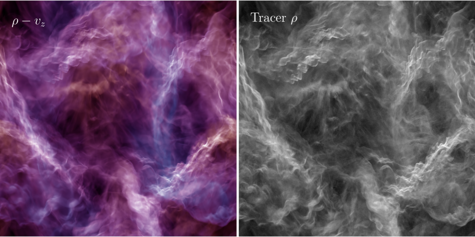
Figure 1: Hydrodynamical simulation of supersonic isothermal turbulence. Shown are a logarithmic projection of the average turbulent fluid density integrated through the $N=512^{3}$ grid (left panel; $0.25<\langle\rho\rangle<4.5$) colorized by the vertical velocity ($0<\varv_{z}<10$ in red; $-10<\varv_{z}<0$ in blue), and a logarithmic projection of the number of tracer particles evolved with the fluid (right panel).

To study dense regions in turbulent clouds, we perform simulations of supersonic isothermal turbulence using a modified version of the hydrodynamics code Athena (Stone et al., 2008). The simulations follow the calculations presented in Robertson & Goldreich (2012), with a few modifications. The calculations simulate an isothermal fluid (with sound speed $c_{\mathrm{s}}=1$) in a unit box (side length $L=1$) with mean density $\bar{\rho}=1$, evolved on either $N=512^{3}$ or $N=1024^{3}$ grids using linear reconstruction and a constrained transport upwind integrator (see Colella, 1990; Gardiner & Stone, 2008). Following Kritsuk et al. (2007), an acceleration field generated with a flat spectrum with power only in the first two $k$-modes drives the fluid. The driving field is constrained to be solenoidal by performing a Helmholtz decomposition in Fourier space on a generic field produced from an appropriate transfer function applied to white noise, using the method described by Bertschinger (2001). The forcing field is applied ten times per crossing time $t_{\mathrm{cross}}=L/(2\bar{\mathcal{M}}c_{\mathrm{s}})$ with an amplitude chosen to maintain a root-mean-squared (RMS) Mach number of $\bar{\mathcal{M}}\approx 5$.

The $N=512^{3}$ simulation is run for fifty crossing times, and the conserved quantities from the simulation grid are recorded ten times per crossing time. After twenty-five crossing times, the simulation is output at a rate of 5000 snapshots per crossing time over a brief duration of one tenth of a crossing time. Afterward, the simulation data are again saved ten times per crossing time. During the last twenty crossing times, the forcing is turned off and the turbulence is allowed to decay. The resulting $\sim 1300$ snapshots provide a wealth of information on the time-dependent properties of supersonic turbulence.

For the $N=1024^{3}$ simulation, we drive the turbulence continuously to maintain an RMS Mach number of $\bar{\mathcal{M}}\approx 5$ and perform our analysis on a single snapshot output after four crossing times. While this higher resolution simulation is driven by different realizations of the forcing field than is the $N=512^{3}$ simulation, we have checked that the statistical properties of both simulations are consistent. We use the results of the $N=1024^{3}$ simulation to verify that our conclusions are insensitive to resolution, as discussed in Section 4 below.

The left panel of Figure 1 shows a visualization of the entire $N=512^{3}$ simulation volume after twenty turbulent crossing times. The image intensity is scaled with a logarithmic projection of the density through the simulation, while the coloration reflects whether the average projected fluid velocity in the vertical direction is positive (red) or negative (blue). The classic features of supersonic turbulence are apparent, with large density inhomogeneities in the fluid spanning $\sim 6$ orders of magnitude in the range $10^{-3}\lesssim\rho/\bar{\rho}\lesssim 10^{3}$. The main focuses of this paper are the structural properties and evolution of the dense regions, which appear bright white in Figure 1.

To assist in our analysis of dense regions in turbulence, we have implemented a new tracer particle scheme into Athena. The details of this numerical scheme are presented in Appendix A. The tracer particles are initially distributed with the grid, but move in response to the fluid velocity interpolated from the grid. Throughout the paper, we use the tracer particles to define dense regions, track their evolution with time, measure the statistical properties of the population of dense regions, and connect the dense regions to the gravitational potential that the turbulent gas would generate given its density structure. Figure 1 shows the number of tracer particles projected through the $N=512^{3}$ simulation volume, scaled logarithmically (right panel). Very similar density inhomogeneities are apparent in both the fluid simulated on the grid and tracer particles. The tracer particles do not represent Lagrangian mass elements (e.g., Genel et al., 2013), but do provide convenient locations for measuring approximate fluid properties interpolated from the grid. The particle interpolation methods are discussed in detail in Appendix B.

3 Dense Regions in Turbulence

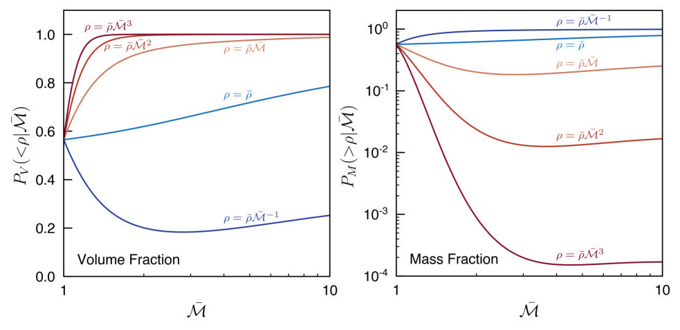
Figure 2: Volume (left) and mass (right) fractions of supersonically turbulent isothermal fluid below and above a given density, respectively. Shown are the volume and mass fractions, defined in Equations 3 and 4 for density thresholds $\rho/\bar{\rho}=[1/\bar{\mathcal{M}},1,\bar{\mathcal{M}},\bar{\mathcal{M}}^{2},\bar{\mathcal{M}}^{3}]$. Most of the volume in supersonic isothermal turbulence lies at densities $1/\bar{\mathcal{M}}\lesssim\rho/\bar{\rho}\lesssim 1$, while most of the mass resides in regions with densities $1\lesssim\rho/\bar{\rho}\lesssim\bar{\mathcal{M}}$.

The simulations described in Section 2 reproduce the well-known phenomenologies of supersonic isothermal turbulence studied extensively in the literature (e.g., Kritsuk et al., 2007; Federrath et al., 2010). The velocity power spectrum is steeper than Kolmogorov, with the high-frequency power-law behaving as $P(k)\propto k^{-\alpha}$ with $\alpha\approx 1.7-1.9$ depending on time variations. In agreement with previous work, the volumetric PDF of density $\rho$ for our solenoidally-driven simulation is close to a lognormal of the form

$$p(x|\bar{\mathcal{M}})dx=\frac{1}{\sqrt{2\pi\sigma^{2}(\bar{\mathcal{M}})}}\exp\left[-\frac{(x-\mu)^{2}}{2\sigma^{2}(\bar{\mathcal{M}})}\right]dx,$$ (1)

with $x\equiv\log\rho/\bar{\rho}$, a dispersion $\sigma$, and the constraint $\mu=-\sigma^{2}(\bar{\mathcal{M}})/2$. Previous authors have found that the dispersion scales with the root-mean-squared (RMS) turbulent Mach number $\bar{\mathcal{M}}$ as

$$\sigma^{2}(\bar{\mathcal{M}})=\log\left(1+b^{2}\bar{\mathcal{M}}^{2}\right),$$ (2)

where the constant $b\sim 0.2-0.5$ (e.g., Padoan et al., 1997; Passot & Vázquez-Semadeni, 1998; Li et al., 2003; Kritsuk et al., 2007; Lemaster & Stone, 2008; Federrath et al., 2010; Price et al., 2011; Konstandin et al., 2012; Molina et al., 2012). In what follows, we will distinguish between the RMS Mach number $\bar{\mathcal{M}}$ that describes the typical bulk random velocity of fluid in the turbulence, and the Mach number $\mathcal{M}$ of individual shocks.

Some implications of the density PDF on the formation and evolution of dense regions in turbulence can be foreseen from integrals of Equation 1, as shown in Figure 2. Displayed are the volume integrals

$$P_{V}(<\rho|\bar{\mathcal{M}})=\int_{-\infty}^{\ln\rho/\bar{\rho}}p(x|\bar{\mathcal{M}})dx$$ (3)

and the mass integrals

$$P_{M}(>\rho|\bar{\mathcal{M}})=\int_{\ln\rho/\bar{\rho}}^{\infty}p(x|\bar{\mathcal{M}})e^{x}dx$$ (4)

indicating the fraction of the volume below and the mass above densities $\rho/\bar{\rho}$, as a function of the RMS Mach number $\bar{\mathcal{M}}$. The volume-filling densities lie at $1/\bar{\mathcal{M}}\lesssim\rho/\bar{\rho}\lesssim 1$, while most of the mass has densities $1\lesssim\rho/\bar{\rho}\lesssim\bar{\mathcal{M}}$. These fractions are only weakly dependent on $\bar{\mathcal{M}}$, and a rough rule of thumb is that for solenoidally-driven turbulence the mass fractions $P_{M}(\rho>\bar{\mathcal{M}}^{\alpha}\bar{\rho}|\bar{\mathcal{M}})\lesssim\bar{\mathcal{M}}^{-\alpha}$. Turbulence driven with compressional modes deviates from the lognormal PDF, and can have somewhat higher velocity- and mass-fractions in dense regions (e.g., Federrath et al., 2008).

The rough factor of $\bar{\mathcal{M}}^{2}$ between the volume-filling density and the mass-occupying density is not accidental, and arises from the compression factor $\mathcal{M}^{2}$ for isothermal shocks. By design, most of the volume and mass of fluid in the simulation move with relative velocities $\varv\sim\bar{\mathcal{M}}c_{\mathrm{s}}$. This connection gives rise to the concept of a first-generation shocked region in turbulence, generated by encounters between regions with the volume-filling density $\rho\sim\bar{\rho}/\bar{\mathcal{M}}$ at the typical relative velocity $\varv\sim\bar{\mathcal{M}}c_{\mathrm{s}}$.

Regions with densities $\rho\gg\bar{\mathcal{M}}\bar{\rho}$ occupy very small volumes ($\lesssim$1 percent) and comprise a small fraction of the total mass of the fluid (a $\sim$few percent) in supersonic isothermal turbulence. Often, the vast majority of computational effort in these simulations is therefore spent elsewhere, on either the regions with volume-filling or mass-occupying densities. The statistical measures typically applied to turbulence simulations, such as the velocity power spectrum, are volume-weighted and therefore largely ignore the densest regions in turbulence.

Since dense regions occupy such a small volume, chance encounters between dense regions are relatively rare. If it survives long enough, a given region with $\rho_{1}\gg\bar{\rho}$ could travel a significant fraction of the simulation volume without colliding with another region with $\rho_{1}>\rho_{2}\gg\bar{\rho}$ if the densities are comparable (e.g., $\rho_{1}/\rho_{2}<\bar{\mathcal{M}}$). This fact bears on whether very dense regions are produced as higher-generation shocked regions, meaning they are produced through generations of collisions between shocks traveling at velocities $\varv\sim\bar{\mathcal{M}}c_{\mathrm{s}}$, or whether they are high-velocity shocked regions where a large relative velocity between the pre- and post-shock regions give rise to a very large density contrast. We discuss this issue in more detail below.

3.1 Measuring the Properties of Dense Regions

Dense regions occupy small fractions of the volume and mass of a turbulent fluid. The three-dimensional structure of turbulence is famously complex, and identifying and characterizing the properties of the densest regions requires additional analysis effort beyond performing the simulation itself. Figure 1 illustrates the complexity of identifying distinct dense regions in turbulence, as dense structures, which appear as filaments in projection, seemingly overlap and do not clearly exist as individual “objects” (e.g., Smith et al., 2016). This complexity arises in part because dense regions are bounded by shocks, and are generated in the interaction of waves in the fluid that have a wide extent in frequency space. The projection of the density field also implies connections between regions along the line of sight, but in many cases these regions can be separated by surrounding regions of substantially lower densities. Nonetheless, the density field appears complex and some methodology for identifying individual shocked regions needs engineering.

The problem of identifying individual dense structures in supersonic turbulence is not unlike the task of cataloging dark matter halos in cosmological N-body simulations (see, e.g., Knebe et al., 2011), with some notable differences. The complexity of the density field in turbulence leads to the “cloud-in-cloud” problems encountered when identifying substructure during halo finding, except with actual clouds. In the absence of self-gravity, turbulence does not have a virial condition to define the extent of regions of interest. Further, in the absence of self-gravity, regions in turbulence are not Lagrangian features. Indeed, the densest regions in turbulence are shocks and material may pass from the pre-shock to the post-shock regions ahead and behind of the shock quickly. The intermittency of turbulence suggests that the properties of dense regions may themselves change on relatively short time scales (e.g., Klessen et al., 2000; Vázquez-Semadeni et al., 2005; Glover & Mac Low, 2007b), and further complicates the analysis of dense regions in turbulence.

To study dense regions, we therefore require methodologies for identifying, measuring, and following them over time. We have engineered some new techniques for accomplishing these tasks, and present those methods in Appendices C, D, and E. The key issues in developing these algorithms include separating distinct regions in the density field, defining a natural frame-of-reference for dense regions that often involve velocity shifts and rotations from the simulation frame and coordinates, and the time-tracking of non-Lagrangian regions whose particle content can evolve over short time scales. These issues do not have unique solutions, but our methods resolve them satisfactorily for the purposes of this work. We refer the interested reader to the Appendices for more detail. Depending on the time step, we typically identify several thousand independent regions with densities $\rho\gtrsim\bar{\mathcal{M}}^{2}\bar{\rho}\sim 25\bar{\rho}$. For simulations with $N=512^{3}$ tracer particles, the dense regions contain $10-10,000$ particles at $\rho\geq 25\bar{\rho}$ depending on each region’s peak density $\rho_{0}\approx(25-300)\bar{\rho}$. We now turn to applying the techniques we have engineered for measuring the properties and time-evolution of these dense regions in supersonic turbulence.

4 Shocked Region Profiles

A prominent feature of isothermal shocks is the $\mathcal{M}^{2}$-contrast in pre- and post-shock densities, and for normal shocks of infinite extent this relation inferred from the Rankine-Hugoniot conditions provides a complete description of the density structure of the flow near the shock (e.g., Shu, 1991). The post-shock structure behind real isothermal shocks are not solely specified by the jump condition, and as is apparent from Figure 1 the individual shocked regions are quite thin with large negative density gradients behind the shock. Using our methods for identifying and measuring the properties of dense regions, we can determine the structure of individual shocked regions and develop a physical model for their density profiles.

Figure 3 shows the density and velocity field near an example shock with peak density $\rho_{0}\approx 230\bar{\rho}$. The one-dimensional profiles are centered about the local peak in the density field and oriented using information from the moment of inertia tensor and the velocity field in the region. Piecewise parabolic (PPI) and Gaussian process (GPI) interpolations of the fluid properties are shown. The “0” subscript denotes the coordinate system of the simulation, and the $x$-direction denotes the primary direction of travel of the shock. This example shocked region is oriented near the $z_{0}$-axis of the simulation volume, such that the bulk velocity of the shocked region is nearly aligned with the $z_{0}$-direction.

In this example, the pre-shock density is close to the mean density and the large density contrast relative to the mean is primarily driven by the $\mathcal{M}^{2}$ change in the $x$-velocity across the shock. This example is therefore a “high-velocity” shocked region. The post-shock density profile eventually declines to near the mean density. As is highlighted by the log-linear scale shown in Figure 3, the post-shock density profile appears roughly exponential.

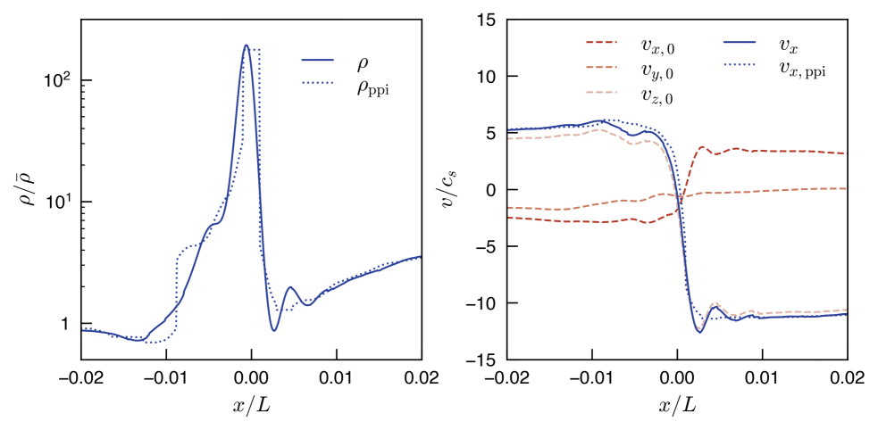
Figure 3: Density (left) and velocity (right) profiles for an example shocked region identified in a supersonic isothermal turbulence simulation. The shocked region was identified from a peak among the tracer particles in the simulation, and the tracers were used to identify the orientation and direction of travel in the simulation volume. The $x$-direction indicates the direction of travel that is primarily orthogonal to the shock front, while the $0$-subscripts indicate coordinates aligned with the simulation volume reference frame. In both panels, Gaussian process (solid lines) and piecewise parabolic (dotted lines) interpolations through the simulation volume are shown. The large density contrast of the shock (left panel) relative to the mean density $\bar{\rho}$ results from its high Mach number ($\mathcal{M}=\varv_{x}/c_{s}\approx 15$), as the pre-shock density is only $\rho\approx\bar{\rho}$. The post-shock density profile appears roughly exponential. This example shocked region is nearly aligned with the $z_{0}$-direction of the simulation volume, and has a primary direction velocity $\varv_{x}\approx\varv_{z,0}$ (solid line, right panel). The velocities of the shocked region in the simulation box reference frame are shown as dashed lines in the right panel. The abscissae in both panels are scaled relative to the simulation box size $L$.

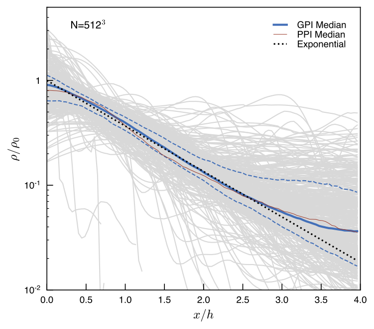
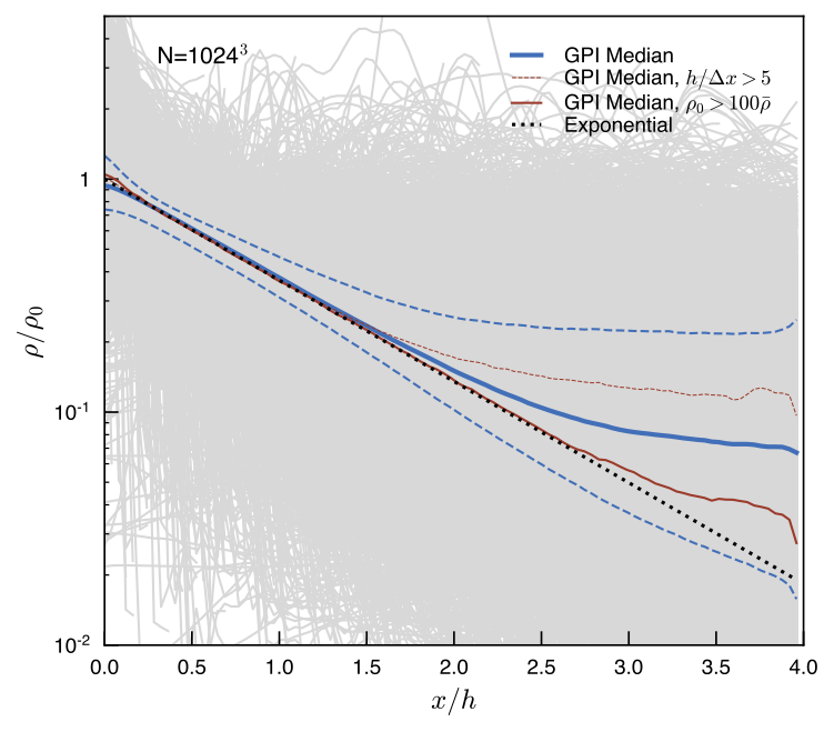
Figure 4: Post-shock density profiles of shocked regions in simulations of supersonic isothermal turbulence. The left panel shows the individual density profiles of hundreds of shocked regions with peak densities $\rho_{0}>25\bar{\rho}$ identified in the $N=512^{3}$ simulation using the tracer particles to separate distinct density enhancements. A path through each shocked region is determined by information from its moment of inertia tensor and velocity field. The post-shock region of the density profile measured along this path is fit with an exponential $\rho\propto\exp(-h/x)$, where positive $x$ corresponds to a post-shock distance from the peak density. Each profile is then rescaled by the scale length $h$ of the exponential, normalized by the maximum of the exponential fit, and then plotted (gray lines). At each position $x/h$ along the axis the median (solid blue line) and inner 68% spread (dashed blue lines) of the Gaussian process interpolation (GPI) profiles can be measured, and compared with a exponential function (dashed black line). The corresponding median profile determined from piecewise parabolic interpolation (PPI) profiles is shown for comparison (thin red line), using the exponential scale length and amplitude determined by fitting to the GPI profiles to rescale each PPI profile. The comparison demonstrates that the median post-shock density profiles is close to exponential out to a distance of at least $x/h\approx 3$, even as individual shocked regions can show substantial deviations and the density profiles of some shocked regions are poorly resolved. The right panel shows the individual shock profiles for $\sim 15,000$ shocked regions identified in the $N=1024^{3}$ simulation (gray lines) with peak densities $\rho_{0}>10\bar{\rho}$. These regions also show exponential profiles (median and inner 68% spread shown as blue lines), but encounter the surrounding background density at smaller $x/h$ than the higher peak density regions shown in the left panel. In the $N=1024^{3}$ simulation, a larger number of the post-shock regions are well-resolved ($h/\Delta x>5$; red dotted line). These well-resolved regions typically have peak densities of $\rho_{0}\sim 10\bar{\rho}$, and encounter the background after $x/h\approx 1.5-2$. In contrast, the densest peaks with $\rho_{0}>100\bar{\rho}$ (thick red line) show exponential profiles to $x/h\approx 3$ before encountering the background density. A physical model for the origin of the exponential profiles shown in both panels is discussed in Section 4.2.

4.1 Average Density Profiles

Given our method for identifying dense regions from the tracer particle distribution, repeating the measurement illustrated in Figure 3 for each shocked region identified in the simulation is straightforward. Information from the moment of inertia tensor defined by the tracer particles associated with each shocked region and their nearby velocity fields can be used to determine the shocked regions’ spatial orientations. The trajectory of each shocked region defines a skewer through the simulation volume oriented roughly perpendicular to the associated shock face, and the properties of the simulated fluid can be interpolated along this skewer using the same interpolation scheme used for assigning properties to the tracer particles. Motivated by the roughly exponential post-shock density profile apparent in the example shocked region shown in Figure 3, we can fit exponentials to the post-shock density profiles of each shocked region and rescale them by their best-fit amplitudes and scale lengths to place them on the same graph.

The left panel of Figure 4 shows the ensemble of density profiles behind the five hundred densest shocked regions identified in a snapshot of the $N=512^{3}$ simulation. Each shocked region profile is rescaled by its fitted scale length $h$ and normalized by the peak of the exponential fit, then plotted as a gray line. At each location $x/h$, the distribution of density profiles can be measured. The median (solid blue line) and inner 68% variation (dashed blue line) of the GPI density profile distribution is plotted in Figure 4, along with an exponential function (dotted black line). The median of the PPI density profiles is shown for comparison as a thin red line, and is rescaled by the GPI profile exponential fit amplitude and scale length parameters. We find that the median post-shock profile of these dense regions is very close to exponential out to at least $x/h\approx 3$. The inferred scale lengths vary widely, from poorly- ($h\sim\Delta x$) to well-resolved ($h\gtrsim 6\Delta x$). Individual shocked regions do show substantial variations from the exponential profile. Some shocked regions are clearly unresolved, and resemble an early solution to the isothermal two-shock Riemann problem with little difference between the pre- and post-shock profile shape (e.g., sharp discontinuities on both sides). Other shocked regions can show exponential post-shock behavior out to roughly five scale lengths. More typically, shocked regions in the simulations follow roughly exponential behavior in their post-shock density profiles for a few scale lengths and then show more complicated density (and velocity) structure well behind the shock as the density profile approaches the average background density.

To further illustrate the exponential density profiles in shocked regions, we can use the $N=1024^{3}$ simulation to study post-shock structures. The right panel of Figure 4 shows $15,000$ density profiles of shocked regions with peak densities $\rho_{0}>10\bar{\rho}$ identified in the higher resolution simulation (gray lines). The previous fitting procedure is repeated, with the resulting median and inner 68% spread in the GPI density profiles shown as blue solid and dashed lines, respectively. These lower density shocked regions show exponential behavior out to $x/h\approx 1.5$, at which point the profiles begin to encounter the background density of the surrounding fluid. Restricting to shocked regions with density profiles resolved with $h/\Delta x>5$ (thin red line) selects out shocked regions with peak densities of $\rho_{0}\sim 10\bar{\rho}$, which typically encounter the background density by $x/h\approx 1.5-2$. This measurement demonstrates that restricting the analysis to well-resolved shocked regions does not substantially change the median exponential behavior. Restricting to the densest shocked regions with $\rho_{0}>100\bar{\rho}$ (thick red line) extends the exponential behavior to $x/h\approx 3$, similar to the densest regions examined in the $N=512^{3}$ simulation (Figure 4, left panel). The $N=512^{3}$ and $N=1024^{3}$ simulations therefore find good agreement for the typical density profiles of shocked regions.

4.2 Exponential Atmosphere Model for Isothermal Shocked Regions

The post-shock density profiles of shocked regions measured in Section 4 typically show a roughly exponential decline. This rapid fall-off of the density distribution can be modeled using a physical picture for the formation and evolution of the isothermal shocked regions forming in the turbulence. In what follows, we present a physical model to explain the general features of dense shocked regions in isothermal supersonic turbulence based on exponential atmospheres.

In turbulence simulations like those studied here, low frequency velocity perturbations are introduced to drive large scale motions of the fluid and resupply energy into the turbulent cascade. These perturbations can lead to substantial velocity variations in the fluid that are compressive on small scales. Large compressive velocities between regions of typical densities can result in high Mach-number shocks.

Initially, these shocked regions can be extremely thin and display sharp density contrasts (unresolved discontinuities) on either side of the density peak. Such regions resemble the initial stages of a two-shock isothermal Riemann problem, where the shock conditions would enforce a $\mathcal{M}^{2}$ density jump relative to the pre- and post-shock regions (with roughly constant densities and velocities) that comprise the local flow. If the local flow were one-dimensional, this shock structure would persist and the width of the dense region would simply increase as the forward and reverse shocks moved into the pre- and post-shock regions. However, given the complexity of the turbulent flow, the pre- and post-shock regions will have density and velocity structure such that the initial pressure balances generating the discontinuities on either side of the dense region will be upset. The density distribution in the post-shock region will re-adjust to accommodate the pressure imbalance, with adjustments occurring over a sound-crossing time across the narrow region. Provided that the original Mach number of the shock is large, material from the pre-shock region with density $\rho_{w}$ will still be encountered at a high relative velocity $\varv_{w}\approx\mathcal{M}c_{\mathrm{s}}$. The post-shock density profile of this region will necessarily adjust to provide a pressure gradient $\nabla p$ that can reach hydrostatic balance with the decelerating force $\rho g$ owing to ram pressure $\rho_{w}\varv_{w}^{2}$ exerted by this on-coming material. We can describe this scenario mathematically by balancing the pressure gradient behind the shock (of density $\rho$) with the ram pressure applied to the shocked region, and write

$$\nabla p=-\rho g=-\rho\frac{\rho_{w}\varv_{w}^{2}}{\Sigma}$$ (5)

where $\Sigma=\int\rho dx$ is the mass per unit area of the shocked region measured along the $x-$direction of travel. Writing $p=\rho c_{\mathrm{s}}^{2}$ we have that

$$\frac{d\rho}{dx}=-\rho\frac{\rho_{w}\varv_{w}^{2}}{c_{\mathrm{s}}^{2}\Sigma},$$ (6)

which gives the exponential solution $\rho(x)=\rho_{0}\exp\left(-x/h\right)$ with

$$h\equiv\frac{c_{\mathrm{s}}^{2}}{g}=\frac{\Sigma}{\rho_{w}\mathcal{M}^{2}}$$ (7)

where $\mathcal{M}$ is the Mach number of the shock.

In this picture, the density structure in the post-shock region provides the pressure gradient needed to counterbalance the incoming ram pressure of the pre-shock material. In a steady state converging flow with constant pre- and post-shock density and velocity, this additional pressure support would be unnecessary and the shocked region would simply behave as a two-shock Riemann problem. The spatial and temporal variations in the turbulent flow that the shock moves through results in the development of a density gradient in the post-shock region. For an isothermal fluid, the corresponding density profile can be roughly exponential. Variations in the velocity and density field, and the non-zero pressure support from the converging flow behind the shock, can lead to deviations from this exponential form, but we expect that the general idea holds. Fluids with different equations of state, or other sources of pressure support like magnetic fields, could display other primary post-shock solutions. We will discuss these possibilities in more detail in Section 9.

4.3 Time-Dependent Exponential Waves

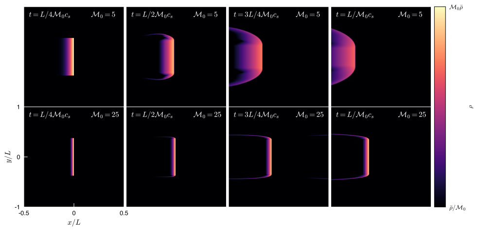
Figure 5: Simulations of exponential waves traveling through a background medium. Shown are thin slices through the density distributions for exponential waves initially traveling to the right with Mach numbers of $\mathcal{M}_{0}=5$ (upper row) and $\mathcal{M}_{0}=25$ (lower row), at times $t=[0,1/4\mathcal{M}_{0},3/4\mathcal{M}_{0},1/\mathcal{M}_{0}]$ (left to right). The logarithmic color map spans the range $\rho=[1/\mathcal{M}_{0},\mathcal{M}_{0}]$. The initial peak density for each wave is set to $\rho_{\star}=\mathcal{M}_{0}\bar{\rho}$, while the background medium has density $\rho=\bar{\rho}/\mathcal{M}_{0}$. The initial surface density of each wave was set to $\Sigma_{0}=0.125\bar{\rho}L$, with corresponding exponential scale lengths of $h_{0}=0.025L$ ($\mathcal{M}_{0}=5$) and $h_{0}=0.005L$ ($\mathcal{M}_{0}=25$). Numerical details of the simulation are discussed in Section 4.4. The simulations demonstrate that the deceleration associated with the ram pressure from the on-coming pre-shock material causes the shocked regions to spread behind the shock and decline in peak density.

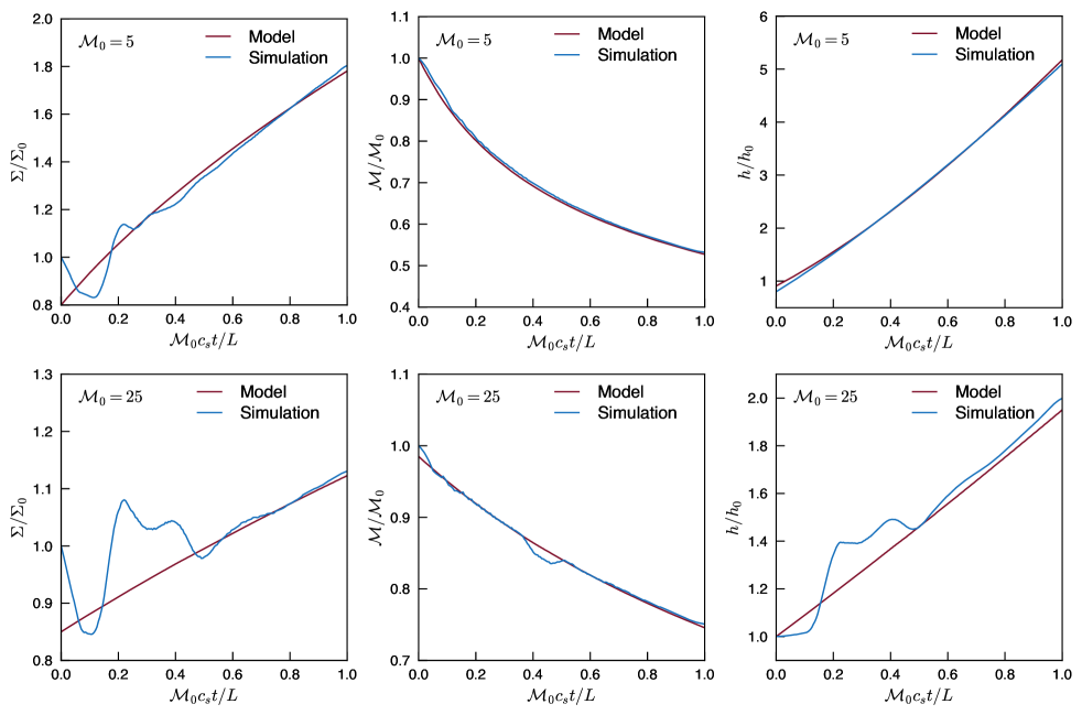
Figure 6: Time evolution of properties of exponential waves traveling through a background medium. Shown are the surface density (left column), Mach number (middle column), and exponential scale length (right column) with time of the waves from the simulations visualized in Figure 5. The properties of the traveling waves measured in the simulations are shown as blue lines in each panel, while the results from the analytical model described in Section 4.3 are shown as red lines. The analytical model for the time dependent surface density, Mach number, and scale lengths of the exponential waves works well, and much of the variation owes to uncertainties in separating the tails of exponential waves from the background medium or relaxation from the initial conditions.

Motivated by the typical post-shock shape of shocked regions in our turbulence simulation, in Section 4.2 we considered an exponential atmosphere model for isothermal shocked regions traveling through a background medium. As the exponential shocked region moves through the background medium, the region could be decelerated by ram pressure from the pre-shock material or an increase in its surface density. The density contrast between the pre-shock material and the density peak will decline as the shocked region decelerates, and as the Mach number of the shock decreases. To get some sense of the time-dependence of an isothermal shocked region traveling through a background medium, we can extend the exponential atmosphere model to account for the effects associated with the region’s deceleration. To do so, we will still approximate the wave as in pressure equilibrium with ram pressure from the background. The region will therefore still have an exponential atmosphere behind the shock, but the scale length of the atmosphere will increase as the mass of the wave grows and the wave decelerates.

First, we can model the time-dependent growth of the surface density of the shocked region. As the shock plows through the surrounding background material, any new material accrued into the shocked region will depend on the background density $\rho_{w}$ and the velocity $\varv=\mathcal{M}c_{\mathrm{s}}$ of the shock. With the ansatz that this material is deposited with some efficiency $\epsilon$, we can write time rate of change of the surface density as

$$\frac{d\Sigma}{dt}=\epsilon\rho_{w}\mathcal{M}c_{\mathrm{s}}.$$ (8)

The value of $\epsilon\neq 1$ in general, as not all of the background material that encounters the shocked region will become permanently entrained. The Mach number of the shock will change with time, but we can still implicitly calculate the time-dependent surface density as

$$\Sigma(t)=\Sigma(t=0)+\int\epsilon\rho_{w}\mathcal{M}c_{\mathrm{s}}dt.$$ (9)

The surface density of the shocked region increases according to the time-integral of the surface density flux of pre-shock material the shock encounters, moderated by some efficiency parameter $\epsilon$.

The deposition of this material will be accompanied by the deposition of relative momentum into the shocked region, and in the case where the background medium is uniform in density and momentum we approximate the rate of this momentum deposition as proportional to the relative velocity of the background medium with respect to the shock times the mass accretion rate into the shocked region. This momentum deposition will reduce the relative velocity of the shock and background. We can balance the rate at which the relative momentum from the background medium is added to the shocked region and the corresponding rate at which the shock decelerates. We can then write

$$\Sigma c_{\mathrm{s}}\frac{d\mathcal{M}}{dt}=-\eta c_{\mathrm{s}}\mathcal{M}\frac{d\Sigma}{dt}$$ (10)

where $\eta$ describes the efficiency of depositing momentum from the background material into the traveling shocked region. Again, $\eta\neq 1$ in general and the efficiency of mass and momentum deposition do not have to be equal (i.e., we have no clear reason to require $\epsilon=\eta$). For constant mass and momentum deposition efficiencies, the solution to Equation 10 is a power-law relation between the Mach number and the surface density,

$$\mathcal{M}(t)=\mathcal{M}(t=0)\left(\frac{\Sigma}{\Sigma(t=0)}\right)^{-\eta}.$$ (11)

If we assume that the density distribution behind the shock maintains instantaneous hydrostatic equilibrium, then the pressure gradient behind the shock will be balanced by the deceleration from the instantaneous ram pressure of the background material. We are making the same assumptions that lead to Equations 6 and 7 above, but now allow for the surface density of the wave to change with time according to Equation 9. The time-dependent scale length can then be modeled as

$$h(t)=\frac{\Sigma(t)}{\rho_{w}\mathcal{M}^{2}(t)}.$$ (12)

As the surface density of the shocked region increases and the Mach number of the shock decreases, the scale length of the post-shock density distribution increases. The material of associated with the shock spreads through the post-shock region. The isothermal jump conditions between the peak density $\rho_{0}$ and the pre-shock density $\rho_{w}$ are maintained, since $\Sigma=\rho_{0}h$ for an exponential density profile.

4.4 Idealized Simulations of Exponential Waves

Testing the above model of shocked regions in the context of the turbulence simulations is difficult because of the complexities of the turbulent flow. Each shocked region encounters differing, time-dependent pre-shock conditions and variations in their locally-convergent velocity field. Instead, we have tried to test the model for shocked regions via controlled simulations of the motion of exponential waves through a background medium. To do this, we use the hydrodynamics code Athena (Stone et al., 2008) to model an exponential wave with initial scale length $h_{0}$ and surface density $\Sigma_{0}$ traveling through a background medium $\rho_{w}$ with an initial relative velocity $\varv=\mathcal{M}_{0}c_{\mathrm{s}}$. The fluid is treated as isothermal with a sound speed $c_{\mathrm{s}}=1$. We perform two such simulations, with $\mathcal{M}_{0}=5$ and $\mathcal{M}_{0}=25$. In both cases, in terms of a characteristic density $\bar{\rho}=1$ we set $\Sigma_{0}/h_{0}=\mathcal{M}_{0}\bar{\rho}$ and $\rho_{w}=\bar{\rho}/\mathcal{M}_{0}$. In terms of a characteristic scale $L=1$, for the $\mathcal{M}_{0}=5$ simulation we set the initial exponential scale length to be $h_{0}=0.025L$. For the $\mathcal{M}_{0}=25$ simulation, we set $h_{0}=0.005L$. The simulations are performed on a three dimensional grid of size $1024\times 512\times 512$ with periodic boundary conditions. For the $\mathcal{M}_{0}=5$ simulation, the spatial resolution of the simulation is set by the cubic cell size $\Delta x=1/256$. For the $\mathcal{M}_{0}=25$ simulation, we use a resolution of $\Delta x=1/1024$ along the shocked region and $\Delta y=\Delta z=1/256$ in the plane of the shock. The exponential shocked regions are initialized as cylinders oriented along the $x$-axis with a diameter of $0.75L$ in the $y$-$z$ plane. We evolve each system until the wave interacts with its own wake after it transverses the volume.

Figure 5 shows the logarithmically scaled map of the density in the $x$-$y$ plane for the $\mathcal{M}_{0}=5$ (upper row) and $\mathcal{M}_{0}=25$ (lower row) simulations, plotted at times $t=0$ (far left column), $t=1/4\mathcal{M}_{0}$ (inner left), $t=3/4\mathcal{M}_{0}$ (inner right), and $t=1/\mathcal{M}_{0}$ (far right). The exponential waves are traveling to the right at an initial velocity of $\varv(t=0)=\mathcal{M}_{0}c_{\mathrm{s}}$ relative to the background medium. The image frames travel at a constant velocity of $\varv=\mathcal{M}_{0}c_{\mathrm{s}}$, initially centered on the shock front. The apparent motion of the shocked regions from right to left reflect their deceleration relative to the background medium (which is traveling through the image frames from right to left with constant relative velocity $\varv=-\mathcal{M}_{0}c_{\mathrm{s}}$). In addition to the deceleration, the decrease in the peak density of the shocked regions and the increase in the post-shock exponential scale lengths are apparent from the density distribution. The density distributions of both shocked regions remain close to exponential for the duration of the simulations. At the edges of the exponential waves bow-like shocks develop (Vishniac, 1994), and the relative size appears larger for the slower shocked region since the vertical spreading of the fluid is limited by the sound speed and the absolute time scale in the $\mathcal{M}_{0}=5$ simulation is prolonged relative to the $\mathcal{M}_{0}=25$ simulation in the bottom panels.

The qualitative evolution of the exponential shocked regions shown in Figure 5 can be quantified from the simulations and compared with the model presented in Section 4.3. We estimate the maximum density $\rho_{\mathrm{max}}(t)$ and exponential scale lengths $h(t)$ of the post-shock regions, and their velocity relative to the background medium, at 100 time steps evenly spaced over the time span $t=[0,1/\mathcal{M}_{0}]$. The time-dependent surface densities of the shocked regions are estimated as $\Sigma(t)=\rho_{\mathrm{max}}h$. Figure 6 shows the surface density (left panels), Mach number (center panels), and exponential scale lengths (right panels) estimated for the shocked regions in the $M_{0}=5$ (upper row) and $M_{0}=25$ (lower row) simulations, normalized to their initial values. These quantities estimated from the simulation data are shown as blue lines. We then use Equations 9-12 as fitting functions to model the time-dependence of the simulation data (red lines). The mass accretion efficiency is taken as $\epsilon=0.88$, while we use momentum efficiencies of $\eta\approx 0.79$ for $\mathcal{M}_{0}=5$ and $\eta\approx 1.0$ for $\mathcal{M}_{0}=25$. Relative to Equation 12, we allow for a mildly nonlinear time dependence in the scale length of $\bar{h}(t)\propto h(t)^{\alpha}$ with $\alpha=0.9$ for $\mathcal{M}_{0}=5$ and $\alpha=0.8$ for $\mathcal{M}_{0}=25$. The early variation apparent in the surface density and scale lengths owes to relaxation from the approximate initial conditions that model the entire exponential waves as traveling with the same initial group velocity, and in inaccuracies in separating the wave from the background medium. These lead to $\sim 10\%$ uncertainties in the measured shocked region surface density and scale lengths, and we account for these errors when computing the time-dependent models shown in Figure 6.

As Figure 6 demonstrates, the model presented in Section 4.3 roughly recovers the time-dependence of the surface density, velocity, and scale lengths of the exponential shocked regions as they are decelerated by the background medium. Physically, this model succeeds because the exponential atmosphere behind the shock responds quickly to the changing ram pressure from the medium ahead of the shock.

5 Shocked Region Lifetimes

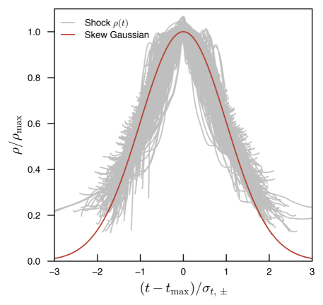
Figure 7: Time-dependence of the peak density of shocked regions in isothermal supersonic turbulence. Shown are the rise and fall of the density in very dense shocked regions ($\rho>25\bar{\rho}$ at their peak) in our turbulence simulation (gray lines), measured in between drivings. The ordinate and abscissa are rescaled by the peak density and by their rise and fall times determined by a skew Gaussian fit (red line, see Equation 13). Dense shocked regions in supersonic isothermal turbulence spread very quickly and rapidly decline in maximum density.

The comparison presented in Section 4.3 between the simulated exponential waves and the time-dependent exponential atmosphere model suggests that the deceleration of shocked regions in supersonic isothermal turbulence will lead to a rapid decline of their peak densities with time. Using the method for tracking shocked regions described in Appendix E, the time dependence of the peak density of simulated shocked regions can be measured.

During the turbulence simulation described in Section 2 the simulation output frequency is increased dramatically after twenty-five turbulent crossing times, such that five hundred outputs are recorded in between applications of the driving field. We identify dense regions from tracers with interpolated densities $\rho\geq 25\bar{\rho}\approx\bar{\mathcal{M}}^{2}\bar{\rho}$ in these simulation outputs according to the method described in Appendix C. Using the population of dense regions identified half-way through this high output-frequency period of the simulation, we track the shocked regions forward and backward with time following the method described in Appendix E. We then have time trajectories of each shocked region’s properties over a short period where the simulation output frequency enables us to follow them reliably. We identify the time at which each shocked region reaches its maximum density over this window, and can then analyze the formation and dispersal of the shocked regions with time.

As anticipated from the model presented in Section 4.3, the individual shocked regions with high peak densities evolve very quickly. Figure 7 shows the rise and fall of shocked regions with peak densities $\rho_{0}\geq 25\bar{\rho}$ (gray lines). For each shocked region, we fit a skew Gaussian of the form

$$\rho(t)=\rho_{\mathrm{max}}\exp\left[-\frac{(t-t_{\mathrm{max}})^{2}}{2\sigma_{t,\pm}^{2}}\right],$$ (13)

where $t_{\max}$ is the time of maximum density $\rho_{\mathrm{max}}$. The quantity $\sigma_{t,\pm}$ equals the rise time $\sigma_{t,-}$ when $t-t_{\mathrm{max}}<0$ and the fall time $\sigma_{t,+}$ when $t-t_{\mathrm{max}}>0$. The rise and fall times are fit separately. We find typical fall times of $\sigma_{t,+}\approx 2-4\times 10^{-3}L/c_{\mathrm{s}}$. The distribution of fall to rise times has a mean of $\sigma_{t,+}/\sigma_{t,-}\approx 1.5$, with a tail extending to $\sigma_{t,+}/\sigma_{t,-}\approx 5$.

The lifetimes of dense shocked regions in the supersonic isothermal turbulence simulation are quite short, comparable to the sound crossing time across the thickness of the post-shock region. The portion of their existence when their density is rising is very short, comparable to the sound crossing time across the cells needed to resolve the density discontinuity at the shock interface with the pre-shock material. The time over which their density declines is only slightly more extended, but substantially longer than the time material takes to flow from the pre- to post-shock regions. The short lifetimes of these shocked regions may bear on models of gravitational collapse in turbulent fluids, and we revisit this measurement in that context in Section 8 below.

6 Deceleration and Spreading of Shocked Regions

The previous sections have outlined an exponential atmosphere model for shocked regions, where the exponential scale length adjusts to the deceleration of the shocked region owing to the on-coming ram pressure of the pre-shock material. This deceleration causes the peak density of shocked regions to decline as the exponential atmosphere spreads behind the traveling shock.

The idealized simulations of exponential waves presented in Section 4.4 illustrate this deceleration and spreading of shocked regions, but demonstrating this effect for shocked regions in supersonic turbulence requires more effort. To this end, we have selected a shocked region tracked over the high-frequency output portion of the $N=512^{3}$ simulation and measured $\sim 2,200$ individual trajectories of the subset of tracer particles continuously associated with the shocked region. As the shocked region travels and spreads, material in the exponential atmosphere is decelerated and gradually lags behind the shock. Relative to the density peak just behind the shock, each parcel of material in the exponential atmosphere will reside at a time-dependent distance $x$ behind the peak. As the material spreads, the distance $x$ of each parcel will typically increase from an initial separation $x_{0}$ to a larger distance after some time $t$.

Figure 8 shows the time-dependent separation between the tracked tracer particles and the moving density peak, $(x-x_{0})/h_{0}$, in units of the initial scale length $h_{0}$ of the atmosphere (gray lines). In Figure 8, the coordinate $x$ corresponds to the direction of travel of the shock and increases in the post-shock direction, and time $t$ is scaled by the sound crossing time across the initial scale length $h_{0}$. The tracers spread at a range of rates as they respond to the deceleration of the shocked region, which owes both to their initial distribution of $x_{0}$ throughout the post-shock flow and to the interpolation scheme used to compute the particle velocities. The mean separation of the tracers and the moving peak of the shocked region is shown as a solid blue line, and the inner 68% of the distribution of separations is shown with dashed blue lines.

To verify that the region spreads in response to the deceleration of the shocked region, we must estimate the expected rate of spreading. For an exponential atmosphere extending to zero density, the density-weighted average distance of material from the peak is equal to the scale length $h$. For finite atmosphere the mean distance from the peak is less than $h$, and for this region that extends for $\sim 2h$ before reaching the background density the mean distance is $\sim 0.7h$. The rate of change of the mean distance from the peak should be proportional to $dh/dt$. If the scale length of the region $h\sim\Sigma/\rho_{0}$, where $\Sigma$ is the surface density of the region and $\rho_{0}$ is the peak density, then we can write

$$\frac{dh}{dt}=\frac{1}{\rho_{0}}\frac{d\Sigma}{dt}-\frac{\Sigma}{\rho_{0}^{2}}\frac{d\rho_{0}}{dt}=\frac{1}{\rho_{0}}\frac{d\Sigma}{dt}-\frac{\Sigma}{\rho_{0}}\frac{d\log\rho_{0}}{dt}.$$ (14)

We can integrate this equation to find the expected spreading of the region $(h-h_{0})/h_{0}$ relative to the initial scale length $h_{0}$ (dotted black line). Equation 14 accounts for how changes in the surface density of the region affect its deceleration in addition to the response to the on-coming ram pressure.

As Figure 8 demonstrates, we find reasonable agreement between the spreading rate measured from the tracer particle positions and the estimate computed from the expected time-dependence of the scale length. We present this measurement as supporting evidence that the exponential atmosphere model provides a useful description of the post-shock flows in shocked regions. We caution that this smooth behavior of spreading only occurs when a region travels through a pre-shock region with relatively constant density and velocity. If instead the region is further compressed to form a higher density sheet, the spreading will cease at least momentarily. Nonetheless, when the pre-shock conditions allow for the exponential atmosphere to develop it spreads at a rate comparable to expectations based on the region’s deceleration.

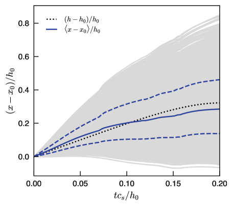
Figure 8: Spreading of post-shock material in a shocked region with time. As shocked regions decelerate owing to on-coming ram pressure from the pre-shock material, their exponential atmospheres spread through the post-shock region. The gray lines show the time-dependent separation $x$ between $\sim 2,200$ tracer particles identified in a shocked region and the location of the region’s peak density, as measured along the direction defined by the associated shock’s trajectory. Plotted are the post-shock locations $(x-x_{0})/h_{0}$ relative to the initial separation $x_{0}$ from the peak, in units of the initial exponential scale length $h_{0}$ of the region, as a function of time $t$ in units of the sound crossing time of the initial region scale length $h_{0}/c_{s}$. The blue solid line indicates the average time-dependent separation, while the dashed blue lines indicate the inner 68% spread in separations. Given the deceleration of the region, the expected growth of the scale length $(h-h_{0})/h_{0}$ and the mean separation of material from the density peak can be estimated from the time-dependent surface density and on-coming ram pressure (dotted black line). The rate of spreading of material in the post-shock region is consistent with expectations computed from the deceleration of the region.

7 Properties of Shock Populations

The preceding analysis has explored the properties of individual shocked regions and the average shocked region properties determined from the population of dense regions identified in the simulation volume. We now turn to the properties of the population of shocked regions as a whole. In analogy with treating dense regions of a cosmological density field in the context of a “halo model”, we will measure some important properties of the dense regions of turbulence in the context of a “shock model” for the population of shocks and associated shocked regions present in the fluid. Dense regions of the turbulent fluid are assigned to individual shocks identified using the method described in Appendix C. The locations of shocked regions are taken to coincide with the their density maxima. Their interior density profiles are assumed to follow the interpolated density at the locations of the tracer particles assigned to them.

7.1 Spatial Clustering of Dense Regions

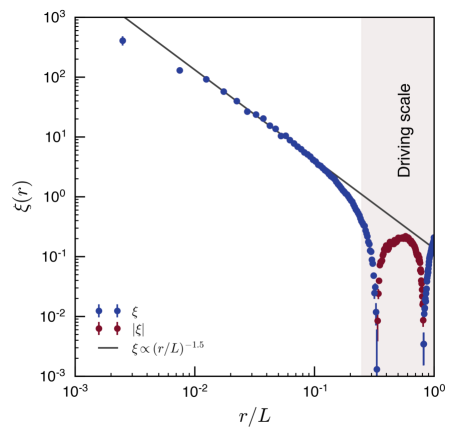
Figure 9: Two-point correlation function of dense shocked regions in supersonic isothermal turbulence. Shown is the correlation function of the density maxima of shocked regions with peak densities $\rho_{0}\gtrsim\bar{\mathcal{M}}^{2}\bar{\rho}$, computed using the Landy & Szalay (1993) estimator, constructed by counting pairs of dense regions in bins of radial separation and comparing them with the corresponding clustering of randomly distributed locations. The correlation function is measured for five statistically-independent times during the turbulence simulation, and then averaged. The error bars indicate the relative uncertainty per radial bin, scaling with the square root of the number of pairs in each. On small scales, the shocked regions are strongly clustered (blue points), with the correlation function scaling approximately as $\xi\propto(r/L)^{-1.5}$ (black line). At scales comparable to the driving scale (gray shaded region), the dense regions become anti-correlated with $\xi<0$ ($|\xi|$ is shown with maroon points).

The density field shown in Figure 1 illustrates some important features of shocked region population in isothermal turbulence. First, the densest regions are spatially clustered. In projection, the sheet-like structures associated with shocks appear filamentary. For turbulence driven at low spatial frequencies, the densest shocked regions occur near the intersections of large-scale velocity perturbations. Second, there are large interior regions in the turbulent fluid, comparable to the driving scale, that are nearly devoid of dense shocked regions. As discussed in Section 3, these regions have volume filling densities $\bar{\rho}/\bar{\mathcal{M}}\lesssim\rho\lesssim\bar{\rho}$ and represent mild rarefactions owing to the large-scale driving modes. Once the shocked regions are identified using the method described in Appendix C, the statistical properties of their spatial distribution should reflect these features.

A useful statistic familiar from cosmology is the two-point correlation function $\xi(r)$ that describes the excess probability for two points pulled from a spatial distribution to be separated by a distance $r$ relative to two points pulled from a uniform random distribution. A convenient estimator for $\xi(r)$ was provided by Landy & Szalay (1993) in the context of galaxy surveys, written as

$$\xi(r)\approx\frac{(DD-2DR+RR)}{RR},$$ (15)

where $D$ represents the locations of data points for which $\xi(R)$ is desired, and $R$ represents the locations of randomly distributed points with the same average number density. The quantities $DD$, $DR$, and $RR$ correspond to data-data, data-random, and random-random point pairs separated by a distance $r$.

To compute $\xi(r)$ for shocked regions with peak densities $\rho_{0}\gtrsim\bar{\mathcal{M}}^{2}\bar{\rho}$ in our turbulence simulation, we identify the locations of maximum density for each region to generate our data sample $D$. We then generate a uniform random point distribution of the same size to populate $R$. The point populations are loaded into k-D trees, allowing for fast neighbor searching to find point pairs separated by a distance $r$. The $DD$, $DR$, and $RR$ pairs are computed, and Equation 15 used to estimate $\xi(r)$. To build signal and to average over high time-frequency variations in the correlation function, the process is repeated for five statistically independent times during the simulation and the measurements averaged. Figure 9 shows the resulting two-point correlation function for dense regions in the turbulence simulation. The correlation increases to small scales, behaving as a rough power law with $\xi(r)\propto(r/L)^{-1.5}$. On scales of a few cells, the correlation weakens somewhat, but this slight turn-down may owe to our shocked region identification method or to resolution effects near the grid scale. On scales comparable to the driving scale of the turbulence the dense regions become anti-correlated, reflecting the presence of large, underdense voids in the density distribution.

Further analogies with the spatial correlations of dark matter halos may provide additional insight. The densest shocked regions in supersonic turbulence are clearly more strongly clustered than the density field, which is itself spatially clustered. The analog in cosmology is the concept of halo bias, where the ratio of the halo and matter correlation functions is $b>1$ for strongly-clustered dark matter halos. The base analytical picture for understanding halo bias is the peak-background split model (e.g., Mo & White, 1996; Sheth & Tormen, 1999; Tinker et al., 2010), where the excess abundance of halos in regions of enhanced background density can be used to estimate their clustering bias relative to the matter field. For turbulence it may be tempting to imagine a “peak density function” $dn/d\rho_{0}$ describing the differential number density of shocked regions as a function of their peak density, or a mass function in analogy to the halo mass function $dn/dM$, which then could be used to estimate the expected bias relative to the turbulent density field. Indeed, similar ideas have been explored before in the context of driven and decaying turbulence (e.g., Smith et al., 2000a, b). The excursion set formalism model of Hopkins (2013a) can be used to compute an analytical model for the clustering of dense regions in turbulence (Hopkins, 2013c) and predicts that $\xi(r)\propto r^{-1}$ on small scales, steepening to $\xi(r)\propto r^{-2}$ on large scales. Our findings appear roughly consistent with these predictions, but our group finding algorithm, which prevents the identification of distinct regions near the grid scale, does not enable us to confirm robustly the origin of the flattening of $\xi(r)$ on small scales. We leave additional comparisons for future work.

7.2 Dense Regions and the Density PDF

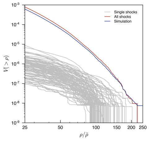
Figure 10: Cumulative density distribution function for supersonic isothermal turbulence, reconstructed from the combined density distributions of individual shocked regions. The volumetric density probability distribution function of supersonic isothermal turbulence is close to lognormal (e.g., Equation 1), and the cumulative density distribution function in turbulence corresponds to the fraction of volume in the fluid above a given density. The density CDF measured from the turbulence simulation (blue) can be compared with the density CDF constructed by summing the individual density distributions (gray lines) of all of the dense regions identified using tracer particles in the simulation (red line). The slight excess of the reconstructed CDF over the simulation CDF results from the allowed overlap of the Voronoi tessellations used to estimate the density PDFs of individual shocked regions. Overall, the excellent agreement demonstrates that the dense tail of the turbulent density PDF corresponds to a population of distinct structures.

The origin and shape of the density probability distribution function (PDF) of supersonic isothermal turbulence influences the star formation process. The roughly lognormal shape of the PDF has been cited as evidence for a statistical origin (e.g., Vazquez-Semadeni, 1994; Padoan & Nordlund, 2002). However the character of the forcing field influences the shape of the PDF on the high-density tail (e.g., Federrath et al., 2008, 2010; Hopkins, 2013b), with compressive modes leading to more high-density material. This result implies that the statistics of the turbulence at high densities retains some memory of the properties of large-scale driving modes, which may argue against the density PDF arising simply from central limit theorem statistical arguments. In the context of this work, where we have identified individual dense regions in supersonic turbulence using the method described in Appendix C and tracked their time evolution following Appendix E, a clear test for our model of dense regions in supersonic turbulence as a collection of distinct traveling waves is whether the density PDF can be reconstructed from their properties.

The turbulence simulation performed on a Cartesian mesh described in Section 2 does display a nearly lognormal density PDF with a width appropriate for its root-mean-squared Mach number. For convenience, we will work with the density cumulative distribution function (CDF)

$$V\left(>\rho\right)=\int_{\rho}^{\infty}\frac{dp}{d\rho}d\rho,$$ (16)

where the density PDF $dp/d\rho$ is normalized to integrate to unity over all densities $\rho>0$. Figure 10 shows the density CDF for our turbulence simulation (blue line), computed by summing the volume in cells above a given density. We examine only the tail of the PDF at densities $\rho>25\bar{\rho}$, corresponding to the threshold density for the tracer particles we associate into groups.

Recovering the density CDF from the individual dense regions in our catalogue constructed from tracer particles is more involved. By design, the density field interpolated at the tracer particle locations varies on scales less that the cell width $\Delta x$. To compute the density CDF from the tracer particles therefore requires us to assign a volume to each tracer particle, and then sum the volume occupied by tracers in our catalogue above a given density. For each group in our catalog we use the Voro++ library (Rycroft, 2009) to construct a Voronoi tessellation about the tracer particle positions, accounting for the presence of nearby low-density tracers that surround each group. Individual tracer particle groups then have their own density CDF $V_{i}(\rho>)$, shown as gray lines in Figure 10 for the one hundred identified groups with the highest peak densities. The total density CDF of the tracer particle groups then corresponds to the sum of the individual group CDFs, e.g., $V(\rho>)=\sum_{i}V_{i}(\rho>)$. The resulting total density CDF reconstructed from our group catalogue is shown as a red line in Figure 10. The agreement between the simulation and reconstructed density CDFs appears quite good, and this result is nontrivial. The slight excess in the reconstructed CDF owes to a combination of our interpolation scheme (here, PPI is used) and permitting overlap of the volumes assigned to the individual groups (tessellating about all tracer particles in the simulation simultaneously would avoid this). Note that in general interpolation schemes that smooth the density field near maxima will not lead to an accurate reconstructed density CDF, as the highest density tail of the CDF will be suppressed.

This demonstrated correspondence between the simulated and reconstructed density CDFs demonstrates that this statistical property of the turbulence arises from the internal structure of distinct regions (for some related analytical models, see Fischera, 2014a, b; Myers, 2015; Veltchev et al., 2016; Donkov et al., 2017). Projections of multiple physically distinct regions along the line-of-sight will then comprise the filaments that produce the observed column density PDF (Moeckel & Burkert, 2015; Chen et al., 2017). Each of the individual regions shown in Figure 10 have been tracked with time during a portion of the simulation, and we have checked that time variations in the simulation density CDF correspond to the evolution of the density structures of individual groups as described in Section 5. We can confirm that the rapid evolution in the peak density of the densest regions discussed in Section 5 indeed corresponds to the time variation in the high-density tail of the PDF (and CDF), as suggested by the models of Hopkins (2013b). Indeed, conceptually the reconstructed density CDF can be considered as an integral over a peak density function $dn/d\rho_{0}$ times the internal density PDF of an individual shocked region with peak density $\rho_{0}$. However, the group-to-group variations apparent in Figures 4 and 10 may suggest a more complex picture. We speculate that variations in the density PDF in turbulence with differing driving mechanisms, or with differing physics (e.g., magnetic fields, adiabatic equations-of-state), will correspond conceptually to changes in the number density and the typical density profile of regions with a given peak density. In self-gravitating regions, this connection appears as the development of a power-law tail in the PDF as the density profile in collapsing regions (Kritsuk et al., 2011; Ballesteros-Paredes et al., 2011; Lee et al., 2015; Burkhart et al., 2017; Murray et al., 2017).

8 Gravity and the Fates of Dense Regions

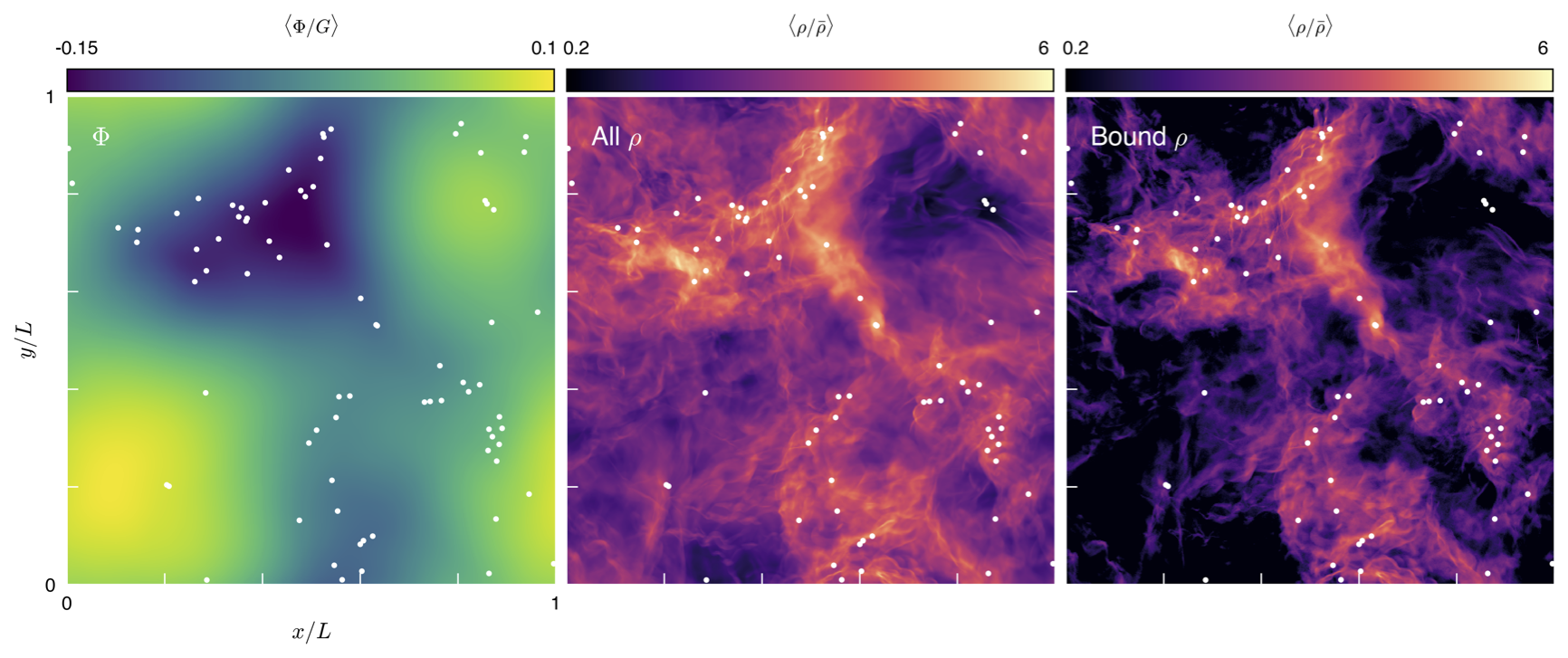
Figure 11: Gravitational potential minima in supersonic isothermal turbulence, and their relation to the density field. Shown are projections of the gravitational potential (left panel; linear projection) and density field (center panel; logarithmic projection) through the entire simulation volume shown in Figure 1. The white points indicate local minima in the gravitational potential, as determined from the potential interpolated at the position of tracer particles. Density maxima correspond to local potential minima, but the global potential minimum in turbulence does not occur at the maximum density (the densest regions occupy very small volumes and contain small mass, see Figure 2). Assuming the turbulence is marginally self-bound to set the value of the gravitational constant, regions in the turbulent fluid that are gravitationally bound to any potential minimum can be identified (right panel; same scale as center panel). Typical gravitationally-bound regions have densities of a few times the mean density, corresponding to the largest density regions that contain substantial mass.

The correspondence between the simulated density distribution of the turbulent fluid and the density CDF reconstructed from individual regions suggests that the bulk properties of high-density volumes in turbulence are tightly connected with the detailed properties of distinct shocked regions. This picture may therefore have important ramifications for models of star formation that involve the turbulent density PDF, such as models that use the density PDF to set the star-formation efficiency of a molecular cloud, the stellar initial mass function, or the core mass function (e.g., Krumholz & McKee, 2005; Padoan & Nordlund, 2011; Hennebelle & Chabrier, 2008, 2011; Federrath & Klessen, 2012; Hopkins, 2013a). As our analysis has illustrated, dense regions are far from static cores and at any given density the density PDF is comprised from differing regions within distinct structures with a range of peak densities. However, to say much more we need to develop some expectations for the evolution of the turbulent gas under the influence of self-gravity.

To compute the gravitational potential of the simulated fluid, we solve the Poisson equation using standard Fourier methods. The Fourier transform of the density field is computed in the three-dimensional volume using the NVIDIA cuFFT library. The potential is calculated by multiplying the density transform by factors of the wave number, and then taking the inverse transform. This process provides the potential $\Phi$ in units of the gravitational constant (i.e., $\Phi/G$). We can then interpolate the potential at the locations of tracer particles to aid in our analysis.

A projection of the resulting gravitational potential is shown in the left panel of Figure 11, along with the density field generating the potential (Figure 11, center panel). The morphology of the potential $\Phi$ follows large overdensities in the turbulent fluid, with broad minima of the potential corresponding to regions with typical density of a few times the background density. This correspondence results from the density structure of the turbulence, since regions with $\bar{\rho}\lesssim\rho\lesssim\bar{\mathcal{M}}\bar{\rho}$ contain a plurality of the fluid mass. While density maxima do lie at local minima in the gravitational potential (shown as white points in Figure 11), the global minimum of the potential does not correspond to a prominent maximum of the density field. The densest regions in the turbulence carry very little mass, and do not dominate the global structure of the gravitational potential sourced by the fluid.

To compute gravitationally-bound regions, the value of the gravitational constant $G$ must be chosen. To set the value of $G$ we assume that the gravitational potential energy in the simulation volume approximately equals the kinetic energy in the turbulent motions, such that the entire box is marginally self-bound. We then have that

$$G\bar{\rho}^{2}L^{5}\approx\frac{1}{2}\bar{\rho}L^{3}\bar{\mathcal{M}}^{2}c_{\mathrm{s}}^{2},$$ (17)

or solving for G we have

$$G=\frac{\bar{\mathcal{M}}^{2}c_{\mathrm{s}}^{2}}{2\bar{\rho}L^{2}}.$$ (18)

Choosing different geometrical factors of order unity in Equation 17 would not change the results of our analysis. With the gravitational constant selected, the tracer particles associated with any potential minima are identified by using a friends-of-friends algorithm similar to that described in Appendix C with a linking length set to the cell width $\Delta x$. The relative potential between the minimum and the maximum potential at the edge of the FOF groups are computed, and then compared with the relative kinetic energy of each particle with respect to the potential minima. Tracer particles with a negative relative total energy are considered to be bound. This process is analogous to that commonly performed when identifying substructure in simulated dark matter halos (e.g., Knebe et al., 2011), except that the geometry in turbulence is more complicated. A logarithmic density projection of the bound regions in the turbulence simulation is shown in the right panel of Figure 11. Most of the mass in bound regions reside in broad potential minima and at typical densities of a few times the mean. The bound regions collectively comprise about $50\%$ of the mass of the entire cloud.

8.1 Time Evolution of the Potential Field vs. Dynamical Timescales

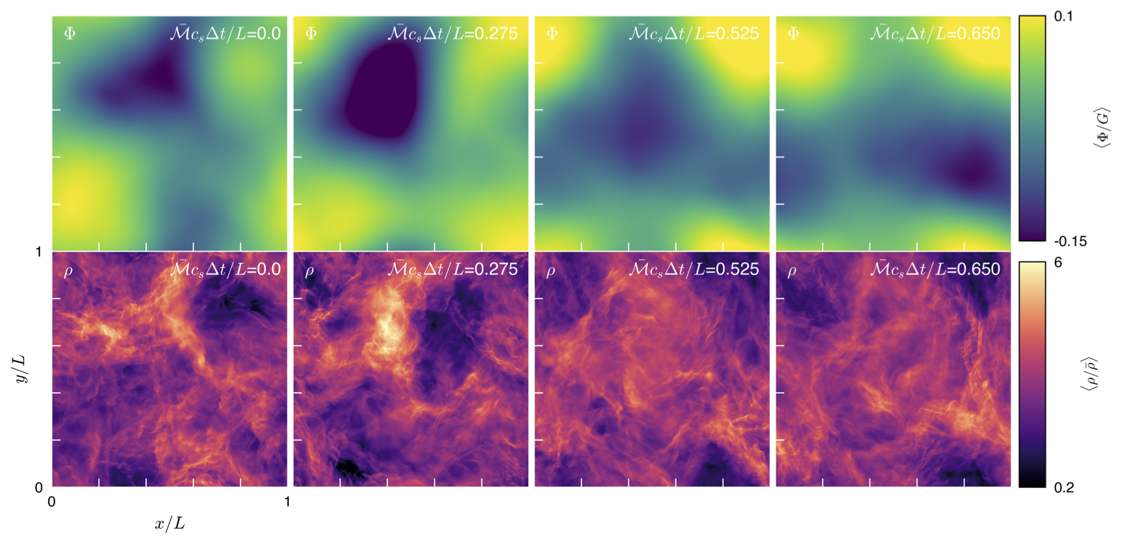
Figure 12: Time evolution of the large-scale potential field in supersonic isothermal turbulence. The gravitational potential (top row; linear projection), sourced by the turbulent density field (bottom row; logarithmic projection), has broad minima that correspond to regions of moderate density that carry a significant fraction of the mass of the fluid. The simulation is evolved forward in time (left to right, in units of the mean Mach crossing time across the simulation volume $t_{\mathrm{cross}}\approx L/\bar{\mathcal{M}}cs$) without the effects of self-gravity to estimate the lifetime of prominent potential minima. Absent the effects of self-gravity, these potential minima would survive only a few Mach crossing times of the dense region sourcing the potential minimum. After this time, the overdensities that source the potential minima disperse (and others reform).

Dense regions in supersonic isothermal turbulence evolve quickly, as discussed in Section 5 above and elsewhere (e.g., Klessen et al., 2000; Vázquez-Semadeni et al., 2005; Glover & Mac Low, 2007b). For dense regions to collapse, their gravitational free-fall time must be shorter than their expansion timescale. In our turbulence simulations where we identified and tracked individual dense regions, the expansion time scale is of order the sound crossing time from the pre- to post-shock regions about the density maxima and is comparable to a few thousandths or one hundredth of the sound crossing time of the whole simulation volume. Dense regions that do collapse and become bound may initially have falling densities or be newly forming during the collapse of a bound region on larger scales. The evolution of the gravitational potential on the scales of the largest bound regions sets the time scale over which denser interior regions must become bound and collapse. Since we found in Section 8 above that large bound regions in turbulence characteristically have intermediate densities $\bar{\rho}\lesssim\rho\lesssim\bar{\mathcal{M}}\bar{\rho}$ that contain substantial mass, we need to monitor the density and potential fields on scales of the simulation volume over time to determine their typical lifetimes.

Figure 12 shows the time evolution of the potential (upper panels; linear projection) and density (lower panels; logarithmic projection) fields in our simulation volume. The potential field is computed from the density field following the method described in the previous Section 8, but the resulting gravitational acceleration is not applied to the fluid with the goal of monitoring the typical lifetime of moderate density regions and their resulting potential minima. Shown are four separate times during the simulation at $\Delta t=[0,0.275,0.525,0.65]$ times the Mach crossing time $t_{\mathcal{M}}=L/\bar{\mathcal{M}}c_{\mathrm{s}}$. The density enhancement in the upper left quadrant at time $t=0$ contains an average interior density close to $\rho\sim\bar{\mathcal{M}}\bar{\rho}$ and sources the broad potential minimum apparent in the corresponding image of the potential field. The initial size of this region is $l\sim L/3$. As the time sequence in Figure 12 shows, the region disperses over a time $\Delta t\sim 0.5-0.6L/\bar{\mathcal{M}}c_{\mathrm{s}}$ that corresponds to $1-2$ Mach crossing times $t_{\mathrm{cross}}\sim l/\bar{\mathcal{M}}c_{\mathrm{s}}$ across the region.

The mass-bearing structures with intermediate densities and their corresponding potential minima have lifetimes that are a few times shorter than the Mach crossing time across the entire box size $L$ but considerably longer than the typical lifetime of the densest turbulent structures. In a real molecular cloud transitioning from low to high mean densities and subsequently undergoing star formation through the gravitational collapse of its dense interior regions, the lifetime of the intermediate density regions will influence how star formation proceeds. For a cloud in rough virial balance, bound regions with intermediate densities $\bar{\rho}\lesssim\rho\lesssim\bar{\mathcal{M}}\bar{\rho}$ will have a collapse time scale of $t_{\mathrm{col}}\lesssim\bar{\mathcal{M}}^{-1}L/c_{\mathrm{s}}\approx t_{\mathrm{cross}}$. If the entire mass of such a region were to collapse to form stars, the star formation efficiency in the entire cloud would be $>10\%$ rather than $\sim 1\%$ (e.g., Krumholz & Tan, 2007). Significant density enhancements within the intermediate density region will collapse on much faster time scales, and if the star formation process of these regions supplies the energy that eventually regulates the cloud’s star formation efficiency such mechanisms must therefore operate on time scales shorter than $t_{\mathrm{col}}\sim\bar{\mathcal{M}}^{-1}L/c_{\mathrm{s}}$.

9 Discussion

This work presents a model where the dense regions of supersonic isothermal turbulence have density profiles that develop approximately exponential atmospheres (Sections 4.1 and 4.2). We present some idealized simulations of exponential waves and an analytical model that shows the time-evolution of dense regions may be understood by accounting for the interaction of the traveling wave with the pre-shock medium (Section 4.3). Observationally, filaments are seen to display a wide range of profiles that are generally modeled with power-laws (e.g., Arzoumanian et al., 2011; Kirk et al., 2013). We note that outside of the smallest scales that may be affected by the beam shape, the density profiles are not far from exponential. In simulations, filamentary profiles have been often been modeled with power-law and Gaussian profiles (Gómez & Vázquez-Semadeni, 2014; Smith et al., 2014, 2016; Federrath, 2016). We expect that exponential profiles will provide comparable quality fits, and benefit from a physical model for their origin. We will examine this issue in future work. We note that filamentary profiles in simulations and observations are frequently treated as a radial profile, whereas our model describes the density profile perpendicular to the shock. The dense regions in our simulations are asymmetrical, with much steeper density profiles (e.g., jumps) ahead of the shock than in the post-shock region and are oriented mostly along the velocity field. Symmetrical fitting of the filament profiles do not account for these features. We note that the power-law radial profile behavior seen in self-gravitating regions of turbulence arises from physics we do not model (Kritsuk et al., 2011; Fischera & Martin, 2012; Heitsch, 2013a, b; Federrath, 2016; Murray et al., 2017; Mocz et al., 2017; Li et al., 2017).

9.1 Caveats to the Exponential Atmosphere Model

A model that approximately describes the properties of dense regions in supersonic turbulence can provide a useful conceptual picture for the formation and evolution of dense shocked regions that may collapse to form self-bound regions. The applicability of the model depends on a host of approximations that we have employed to make the problem tractable, and our numerical simulations have limitations. We now examine some of these assumptions and limitations, and attempt to evaluate, at least qualitatively, how they might affect the realism of the physical picture presented in this work.

9.1.1 Equation of State

An immediate concern is the applicability of isothermality to dense regions of observed molecular clouds. The radiative efficiency of shocks in dense gas motivates the isothermal assumption, but the gas does not have to remain perfectly isothermal. If the adiabatic index $\gamma>1$, then the additional pressure support of the fluid during compression will resist the large amplification of the density possible in isothermal shocks. According to the Rankine-Hugoniot conditions, the factor of $\sim 4$ density amplification in individual adiabatic shocks may have a variety of implications to the model. In terms of the volumetric density PDF, regions of high density can still develop through (relatively larger numbers of) successive generations of shocked regions (Scalo et al., 1998; Federrath & Klessen, 2012). But how will the structure of individual shocked regions change? The alteration will depend on whether the shocked regions remain thin enough that the time for their interior structure to adjust to the ram pressure force applied by on-coming material remains shorter than the time for them to travel an appreciable distance or their mass to change significantly. The primary influence on this thickness will be the value of $\gamma$, but if the adiabatic index is low enough to allow a fast response to ram pressure variations at the shock front then the shocked region structure will reflect the pressure gradient required under the stiffer equation of state to balance the ram pressure force. Indeed, previous simulations of turbulence that include radiative cooling suggest that the post-shock region will remain close to isothermal behind a radiative shock front (e.g., Pavlovski et al., 2006).

9.1.2 Magnetic Fields

We do not attempt to generalize our results to MHD turbulence. Models for the statistical properties of strong, incompressible MHD turbulence have been developed (Goldreich & Sridhar, 1995) and examined in the context of large scale numerical simulations (Beresnyak, 2011, 2014, see also Perez et al. 2012). The shock compression of regions threaded by weak magnetic fields will lead to an amplification of the field and an increase in the magnetic pressure support within the fluid, thereby changing the balance between internal pressure and exterior ram pressure. The density PDF of MHD turbulence does display an approximately lognormal distribution (e.g., Ostriker et al., 2001), which suggests large density inhomogeneities that would allow for dense shocked regions to encounter a low density background a short time after their formation. However, their pressure support and internal structure could differ significantly from isothermal hydrodynamic shocks. Analysis of filaments in MHD simulations show that the central density contrast of the filaments are reduced, but that the overall profile of the filaments may not change substantially (Federrath, 2016).

9.1.3 Limitations of the Simulations

The numerical simulations of supersonic turbulence we present have limitations. Given the reconstruction scheme used, the first scale length of the exponential atmosphere of the densest shocked regions ($\rho\gtrsim 50\bar{\rho}$) will not be well-resolved. As Figure 4 indicates, our ability to study the density profile very near the shocked region peaks (e.g., $x\lesssim 0.5h$) will affected by resolution. However, the exponential profile appears to be consistent with the actual measured density profile of shocked regions out to typically $x\sim 3h$ where even dense shocked region atmospheres have been captured by $\gtrsim 10$ cells and simulations in the literature do not show strong variations in filament profiles with resolution (e.g, Federrath, 2016). We also note that the inertial range of $N=512^{3}-1024^{3}$ simulations of $M\approx 5$ turbulence is known to be limited (e.g., Kritsuk et al., 2007; Federrath et al., 2010). Increasing the numerical resolution of the simulations can obviate or mitigate these limitations.

9.2 Outstanding Issues

In this work, we have used supersonic isothermal turbulence to generate a set of dense regions whose properties we have measured and modeled physically. The methodology for generating the turbulence and using it as a model for molecular clouds is well-established, and we follow the approach of previous works discussed in Section 1. Once self-gravity begins to operate, we expect the subsequent collapse to follow the picture laid out by Murray & Chang (2015) where the adiabatic heating mechanism we identified in Robertson & Goldreich (2012) changes the nature of the turbulence in the clouds as they condense. Adiabatic heating moderates the collapse, and gives rise to the density and velocity structure measured in simulations that include self-gravity and follow the collapse of individual regions to small scales (e.g., Kritsuk et al., 2011; Murray et al., 2017; Mocz et al., 2017; Li et al., 2017). Once star formation commences, the input of feedback in various forms (Matzner & McKee, 2000; Mac Low & Klessen, 2004; Krumholz & Tan, 2007; Federrath, 2015; Raskutti et al., 2016; Rosen et al., 2016; Li et al., 2017) may influence the overall star formation efficiency by dispersing low density material. Although the collapse to high densities occurs on short (e.g., several free-fall) time scales, the cloud itself could persist much longer if its material is replenished. An important issue then is to determine how the persistent turbulent flow in star-forming molecular clouds originates or is organized on large scales.

A possible avenue is the density enhancement of gas passing through potential perturbations as it orbits in the galactic disk, such as in spiral arms (Shu et al., 1973), that leads to a convergent flow (e.g., Hartmann et al., 2001). Various mechanisms have been envisioned for using the response of the gas in spiral features to promote the formation of molecular clouds, such as agglomeration, cooling and thermal instability, large-scale Jean instability, and cloud-cloud collisions (Kim et al., 2008; Dobbs, 2008; Dobbs et al., 2008; Dobbs & Bonnell, 2008; Tasker & Tan, 2009; Dobbs et al., 2015), and to drive turbulence (e.g., Kim et al., 2006). Using the response of gas to galactic potential perturbations to understand the initial conditions for persistent turbulent flows of molecular clouds may be promising if it can explain how the size-line width relation of originates on large scales and determine what sets the maximum size of clouds. Once molecular clouds are organized from more diffuse galactic disk material and placed on the size - line width relation on the largest scales, the properties of the resulting turbulent flow, adiabatic heating in interior regions undergoing gravitational collapse, and possible input from feedback may combine to provide a complete picture for star formation on large scales. We leave analysis of this speculation for future work.

10 Conclusions

Astrophysical fluids often display turbulent motions, owing to the large Reynolds numbers and low viscosities typical of conditions observed in molecular clouds, neutral hydrogen gas, and even the ionized interstellar medium. The properties of supersonic isothermal turbulence especially influence dense molecular clouds with large radiative cooling efficiencies and bulk motions with velocities in excess of the thermal value. As a result, the statistical properties of supersonic turbulence have provided the core of analytical theories of the formation rate of populations of stars. Owing in part to the complexity of turbulence, these models have largely emphasized the statistical properties of the fluid rather than the character of individual dense regions that may collapse to form stars.

Our work adopts a new approach that aims to describe the properties of the dense regions in supersonic isothermal turbulence that serve as the sites of star formation. Our model is grounded by a distinguishing feature of supersonic isothermal turbulence, that the origin of large density contrasts in the turbulent fluid is from strong shocks with Mach number $\mathcal{M}$ where the density in post-shock regions is enhanced by a factor $\sim\mathcal{M}^{2}$ relative to the pre-shock material. The volume of supersonic isothermal turbulence occupied by dense fluid is small, and as a result after their formation these shocked regions rapidly encounter lower density material. The low density external medium applies a ram pressure to the shocked regions, and the thinness of the dense shocked regions implies that the internal structure of the isothermal shocked regions will quickly adjust such that its pressure (and density) gradient balances the force applied by the ram pressure. Using this local force balance at the front of the shocked region, we model the structure of the fluid behind the shock as an exponential atmosphere whose rapidly declining density reflects the pressure gradient necessary to counter the force from the ram pressure applied across the face of the shocked region.

We use simulations of supersonic isothermal turbulence to compare our analytical model with detailed hydrodynamical calculations of the fluid structure. We study the density structure of shocked regions, and find consistency between their density distributions and our exponential atmosphere model. We then use idealized simulations to study the evolution of exponential shocked regions traveling through a low-density background, and find that we can describe the time-dependent structure of the exponential shocked regions in terms of the integrated deceleration of each region by the ram pressure force applied by the low density material, the corresponding hydrostatic balance of this force and the pressure gradient behind the shock, and the mass of the background fluid accreted into the shocked region.

After determining that the exponential atmosphere model appears consistent with the structures of isothermal shocked regions in our idealized and supersonic turbulence simulations, we use the results of the model to infer some additional extensions. Using the catalog of shocked regions constructed from our tracer particle distributions, we measure the correlation function of dense regions and find that it scales as a power-law $\xi(r)\propto r^{-1.5}$ over scales between a few times the grid size to the driving scale. Dense regions become anti-correlated at about the driving scale, possibly owing to the large scale rarefactions in the fluid on these scales. Computing the volumes associated with each dense region from cell tessellations about the tracer particle locations allows us to demonstrate that the dense tail of the cumulative density function can be entirely accounted for through the sum of individual shocked region structures.

We compute the gravitational potential of the turbulent fluid, and determine the characteristic density and size of bound regions for a turbulent cloud marginally bound on a scale comparable to the box size. The global minimum of the gravitational potential of the turbulent fluid corresponds to a region of moderate density, with a volume large enough to contain substantial mass (a few tens of percent of the total cloud). The densest regions in the turbulence correspond to local (not global) potential minima but do not contain substantial mass as distinct regions. Without the influence of gravity the larger overdensities will dissipate on their local Mach crossing time, which we find to be of order $t_{\mathrm{col}}\sim\bar{\mathcal{M}}^{-1}L/c_{\mathrm{s}}$.

As this model for the properties of individual shocked regions in supersonic turbulence is developed, extended, and modified, the time-dependent evolution of the structure of dense regions in turbulence can be utilized to describe the observed properties of molecular clouds. Descriptions of the statistical properties of turbulence and the structural properties of individual dense regions can be employed together to improve our physical picture of star formation in supersonically turbulent gas.

Appendix A Tracer Particle Scheme

To assist in studying the formation and evolution of shocked regions in our turbulence simulations, we have implemented a new tracer particle scheme into Athena. We begin by placing a single tracer particle in the center of each cell at the start of the simulation. The velocity and position of the particles are updated using a second-order Verlet-like scheme, and during the simulation the properties of the fluid at the tracer particle locations are interpolated from the grid using a triangular-shaped cloud (TSC) scheme (e.g., Hockney & Eastwood, 1988). The tracer particle data are written along with the grid data for each simulation snapshot.

Over each time step $\Delta t$, the tracer particle positions $x$ are evolved according to

$$x_{\mathrm{t}+\Delta\mathrm{t}}=x_{\mathrm{t}}+\frac{1}{2}\left(\varv_{\mathrm{t}+\Delta\mathrm{t}}+\varv_{\mathrm{t}}\right)\Delta\mathrm{t},$$ (A1)

where the particle velocities $\varv$ are computed from the interpolated fluid mass and momentum densities at times $t$ and $t+\Delta t$. The Courant condition that determines the time step criterion in Athena is also altered to account for the tracer particle motions. When calculating the time step from the Courant condition, the particle velocities are treated analogously to the signal speed calculated from the fluid properties on the grid. Since the particle properties are interpolated from the grid, the alteration to the Courant condition typically only has a minor effect on time steps.

The tracer particle scheme is parallelized in a manner that reflects the communication structure of Athena as a whole. Each local grid, typically evolved by its own parallel process, is assigned a list of local tracer particles. As particles cross grid interfaces, the grid boundary conditions are applied. If the tracers cross an internal boundary between grids owned by different MPI processes or periodic boundaries on the exterior of the computational volume, they are marked, packed into communication buffers, and then exchanged with adjacent grids via non-blocking MPI_Isend(). Grids receive tracers flowing from adjacent grids on a first-come-first-served basis using MPI_Waitany() and MPI_Irecv() calls. The process is repeated to allow for tracers to cross multiple cell faces (a rare occurrence very close to grid edges and corners). If necessary, the tracer positions are then adjusted appropriately for wrapping across periodic boundaries.

Appendix B Interpolation of Tracer Properties

Godunov-style grid-based fluid simulations use reconstruction methods to provide subcell gradients in the fluid, and thereby improve extrapolations to the cell interfaces where the Riemann problems are computed for flux calculations. The values of the fluid on the grid are often stored as central cell-averages, and correspond to integrals over the fluid shape within the cell in a finite-volume approximation. Given the irregular distribution of the tracer particles, interpolation methods are used to estimate the fluid properties at the tracer locations. In computing the simulations presented here, to evolve the tracer particle positions and velocities the fluid properties simulated on the grid are interpolated at the tracer particles using the TSC method. Since this interpolation method acts like a kernel-weighted estimate of the fluid properties at locations intermediate between the grid locations, the fluid properties are smoothed on scales comparable to the grid spacing. A consequence of this interpolation scheme is that the tracer particle properties near extrema in the fluid are smoothly truncated. If the particles are to be used to reconstruct the statistical properties of the fluid simulated on the grid, such as the density probability density function (PDF) measured volumetrically, then the extrema must be preserved. To maintain these features of the fluid properties interpolated at the tracer particle locations, we require different interpolation schemes than TSC. A trivial choice would be to use a nearest grid point method, but this method reduces the order of the interpolation and does not reflect the assumed model of the original grid simulation that subcell gradients in the fluid properties exist. Below, we introduce two additional interpolation methods that work well and are comparable in quality, and better capture the extrema in the simulated fluid properties.

In re-interpolating the fluid at the tracer particle positions, we treat the tracers as sample locations for constructing new approximations to the smooth fluid properties between grid cells. We do not treat the tracers as Lagrangian elements (see, e.g., Genel et al., 2013), and do not assign unique mass elements to tracers in an attempt to follow parcels of gas. However, since we are concerned primarily with the development and evolution of shocked regions (which are not Lagrangian structures) this issue poses no serious difficulty. When necessary and discussed in more detail below, shocked regions are followed using successive generations of tracer particles that move through the structures of interest. Shock fronts can be identified based on the time-dependent density of the fluid as sampled by the tracers.

B.1 Piecewise Parabolic Interpolation

Spatial reconstruction using piecewise interpolation is a core feature of modern Godunov-based fluid dynamics methods. The piecewise parabolic method (PPM; Colella & Woodward, 1984) is one such scheme that provides a third-order accurate reconstruction on a one-dimensional grid by using cell averages across a stencil to constrain the assumed parabolic shape of the fluid properties interior to each cell. PPM is often used in grid-based simulations when extrapolating the fluid properties at the cell interfaces to compute the input states for a Riemann problem during the hydrodynamical time integration. This treatment is approximate, and the reconstruction in each direction is usually treated independently, such that the PPM reconstruction is determined from a grid-aligned stencil of cells in a single row or column. However, suitable averages of one-dimensional PPM reconstructions in each direction can be taken to provide an approximate three-dimensional interpolation scheme that we call piecewise parabolic interpolation.

Consider a one-dimensional PPM reconstruction $q_{i}(x_{i})$ providing the assume parabolic shape of the fluid at location $x_{i}$ within a cell along direction $i\in[x,y,z]$. For $q_{i}$, we adopt the same PPM reconstruction used by the FLASH code and refer the reader to Fryxell et al. (2000) for details. To construct an estimated three-dimensional interpolation $q(x,y,z)$ within a cell centered at $[0,0,0]$, we then compute a simple linear interpolation between the $x-$, $y-$, and $z-$interpolations using the heuristic

$$\phi = \arctan\left(|x|,|y|\right)$$

$$\theta = \arctan\left(|z|,\sqrt{x^{2}+y^{2}}\right)$$

$$q_{xy} = q_{x}\left(1-\frac{2\phi}{\pi}\right)+q_{y}\frac{2\phi}{\pi}$$

$$q(x,y,z) = q_{xy}\left(1-\frac{2\theta}{\pi}\right)+q_{z}\frac{2\theta}{\pi}.$$ (B1)

We refer to this as Piecewise Parabolic Interpolation (PPI) in the text. We use the same slope limiters and monotonicity constraints as Fryxell et al. (2000), which result in a constant reconstruction within cells at local extrema. Interpolations along the $x-$, $y-$ or $z-$directions relative to the cell centers reduce to the corresponding one-dimensional PPM reconstructions. Other three-dimensional averages of the one-dimensional PPM reconstructions are possible and may prove more advantageous for other applications.

B.2 Gaussian Process Interpolation

When interpolating the fluid properties from the grid, using a method constrained to reproduce the fluid properties at the grid centers can help reproduce extrema. Such a method would interpolate between the cell-averaged quantities of the original fluid reconstruction, but may not reproduce those quantities when averaged over the grid. If the interpolation is smooth then such a method can overshoot extrema on the original grid over a portion of a grid cell, but appropriate choices can make such overshoots small in practice.

A smooth interpolation scheme that can be constrained to pass through central cell values is Gaussian process interpolation (Rasmussen & Williams, 2006). If we treat the cell values in a simulation as realizations from a Gaussian process, then we can interpolate between cell values by defining a model for the covariance between nearby cell values and computing the mean of the Gaussian process everywhere (e.g., Reyes et al., 2016). The method is intrinsically multidimensional, and does not require information about the directionality of the interpolation.

Consider $f(x)$ to be the realization of a function at the cell center locations $x$. To interpolate between $x$ and some other location $x_{\star}$, one can treat the function as a Gaussian process and use the estimate

$$\langle f(x_{\star})\rangle\simeq k(x_{\star},x)k^{-1}(x,x)f(x)$$ (B2)

where $k(x_{a},x_{b})$ is a model for the covariance matrix between the function values at locations $x_{a}$ and $x_{b}$, and $k^{-1}$ is its inverse. Note $k^{-1}(x,x)$ is computed from the covariance of the function as sampled at grid locations $x$, and has a size $n_{x}\times n_{x}$ where $n_{x}$ is the number of contributing nearby grid cells. The interpolants $\langle f(x_{\star})\rangle$ are therefore weighted sums of the function values at the cell centers, but the product of the covariance matrix with its inverse ensures that $\langle f(x_{\star})\rangle\to f(x)$ as $x_{\star}\to x$.

The implementation of this scheme involves choices for the set of cell centers contribute to the interpolant at each location $x_{\star}$ and the form of the covariance function. A common model for the covariance function is a Gaussian

$$k(x_{a},x_{b})=\frac{1}{\sqrt{2\pi l^{2}}}\exp\left[-\frac{(x_{a}-x_{b})^{2}}{2l^{2}}\right]$$ (B3)

where $l$ is a typical correlation length and $|x_{a}-x_{b}|$ is the vector magnitude between the (three-dimensional) locations $x_{a}$ and $x_{b}$. Nominally, given this covariance function all cells in the simulation would contribute to the Gaussian process interpolation at any interior location. Since the contributions of cells at a distance more than the correlation length are exponentially suppressed, only relatively nearby cells within a few correlation lengths need to be considered. In practice we choose a correlation length $l=\sqrt{3}\Delta x$, where $\Delta x$ is the cell width, and consider contributions from cells at distances $|x-x_{\star}|\lesssim 4l$. Our interpolation stencil is therefore $9^{3}=729$ cells, and our inverse correlation matrix has $729\times 729=531441$ elements. However, the regular spacing of the grid allows for $k^{-1}(x,x)$ to be computed only once and reused for each interpolation. We use the Intel Math Kernel Library implementation of the Cholesky decomposition to perform efficiently the matrix inversion. Equation B2 is then evaluated for all $N=512^{3}$ or $N=1024^{3}$ tracers at every snapshot of interest.

B.3 Comparison of Interpolation Methods

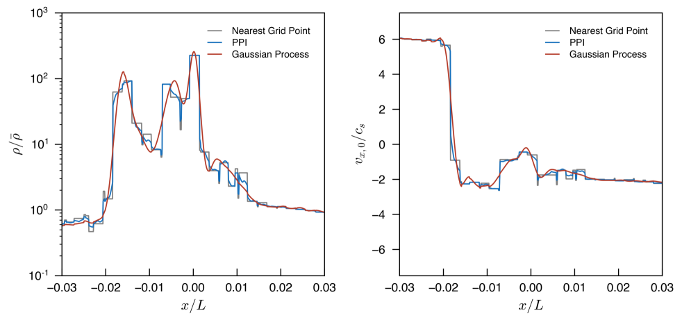
Figure 13: Comparison of interpolations methods. Shown are the Nearest Grid Point (NGP; gray), Piecewise Parabolic (PPI; blue line), and Gaussian Process (GPI; red line) interpolations of the density (left) and $x_{0}$-direction (grid-aligned) velocity (right) field near a dense shocked region with $\rho\approx 230\bar{\rho}$ in the $N=512^{3}$ simulation. The trajectory of the interpolation is not aligned with the simulation grid, such that the Nearest Grid Point interpolation can show large variations on scales smaller than the grid scale $\Delta x=L/512$. The PPI method matches the NGP method near the density maximum , but varies more smoothly than NGP. The GPI method is smoother than PPM, as it kernel-weights information from a $9^{3}$ stencil about each position, but provides a density estimate near extrema within about $10\%$ of the NGP value.

The PPI (Section B.1) and GPI (Section B.2) methods for estimating the simulated fluid properties reconstructed at the positions of tracer particles provide two approaches with complementary advantages. Figure 13 compares the reconstructions provided by the two methods (PPI in blue, GPI in red), along with the Nearest Grid Point method (gray), for density (left) and velocity (right) interpolation along a skewer oriented perpendicular to a dense shocked region identified in the turbulence simulation. The PPI method preserves the behavior of NGP interpolation in that density maxima are flattened to a constant within a cell, which allows for the recovery of the densest part of the density PDF (see Section 7.2). The GPI method The GPI method provides a smoother interpolation, which is advantageous in determining which tracer particles to assign to a dense region (Section C) and in measuring density profiles behind shocks (Section 4.1), but still recovers the value of the density maximum to within $\approx 10\%$. We note that the small-scale variations on scales less than the grid scale $\Delta x=L/512$ in the NGP and PPI methods arise from the oblique of the interpolation path relative to the grid.

Appendix C Group Finding Algorithm

Calculating the properties of individual dense regions in an Eulerian simulation is straightforward at any specific time. For an isothermal fluid, shock fonts may be simply identified by their large density gradient upwind from a large density enhancement. Regions with a large density enhancement (e.g., $\rho/\bar{\rho}>M$) must be generated by shocks. However, if one wants to monitor the formation and evolution of dense regions an Eulerian scheme presents some difficulties. When tracking the history of an individual shocked region back in time, the associated shock will inevitably have originated from the compression of two distinct regions. The history of the shocked region before this point will become indeterminate. Very dense shocked regions in isothermal turbulence are themselves created from the interaction of lower density shocked regions, and following the formation of such higher generation shocked regions quickly becomes difficult in an Eulerian simulation.

By using tracer particles, we can monitor the motion of particles (at least momentarily) associated with a given shock. Since the tracers move through the shocks, we can use successive generations of tracers to follow the motion of a shocked region with time and reconstruct its history (see Section E below). To achieve this, we must have a robust method for associating groups of tracer particles in shocked regions. There are a variety of possible methods and we have tried several, but we find the following algorithm to work well in practice.

Since we are interested in shocked regions, we first select particles denser than a chosen threshold $\rho_{\mathrm{thresh}}$ to incorporate into distinct regions. This simple selection essentially defines the particle membership of regions we study, but to follow the formation and evolution of the shocked regions we need to organize the tracers into distinct groups. Our method for organizing the dense tracers into individual shocked regions is a friends-of-friends (FOF) group finding algorithm (e.g., Huchra & Geller 1982), where we separate tracer particles into FOF groups based on their spatial proximity. Regions whose closest tracers are separated by more than a linking length $b$ are considered to be distinct. We choose the linking length to be of order the expected mean inter-particle separation for a density of $\rho\sim\rho_{\mathrm{thresh}}$. By conditioning the FOF membership on density, we avoid using the linking length as an estimator for the density near the bounding surface of the shock. Instead, the linking length is simply used as a metric to determine whether two shocked regions are proximate or distant. This feature of our algorithm avoids some of the FOF group finding pathologies discussed in More et al. (2011) in the context of cosmological N-body simulations.

Our algorithm for identifying density-conditioned FOF groups is as follows:

1. Select Tracers Above a Given Density Threshold. We select tracers above a density threshold $\rho_{\mathrm{thresh}}$ to define the spatial extent of shocked regions. The tracer densities are computed by interpolating the local fluid properties, and placing a condition on the tracer densities for FOF group membership amounts to selecting regions within isodensity contours sampled at the tracer locations. Conditioning the group membership on density also reduces the number of tracers that need to be processed, which reduces the computational time of the rest of the algorithm.

2. Construct a Graph. The separation of dense tracers into distinct regions requires an evaluation of their spatial distribution. More specifically, we require a method for determining whether tracers are proximate or well-separated. By constructing a graph of the tracers, the distances between nearby tracers are recorded and can be compared with a metric to group tracers based on their proximity. If we consider the tracer positions as vertex locations in the graph, we generically do not know which edge connections between vertexes with lengths $l<b$ will comprise connections between members of a shocked region. Constructing a complete graph of the tracer distribution would guarantee that all desired connections would be identified, but constructing such a graph for $N$ tracers requires $O(N^{2})$ operations and is computationally prohibitive. Instead, we construct a graph of the tracers where each tracer (vertex) is connected by some number $N_{\mathrm{ST}}\ll N$ edges to other vertices. We require these edges to be among the shortest available connections, since all edges with lengths $l>b$ will eventually be discarded once the FOF groups are constructed. A nearest neighbor search is therefore performed, with the shortest $N_{\mathrm{ST}}$ edges for each vertex identified. To construct this graph, a kD-tree of the tracer positions is generated and utilized to perform rapidly the neighbor searching. A value of $N_{\mathrm{ST}}\sim 10$ is chosen to provide a large connectivity between regions (we do not require that all tracers are connected in the graph, we just require that all tracers closer than a distance $b$ are connected). Picking too small a value of $N_{\mathrm{ST}}$ can result in disconnected regions whose closest $N_{\mathrm{ST}}$ neighbors are self-contained, while picking too large a value of $N_{\mathrm{ST}}$ increases the computational cost of the algorithm. Some of the connections may have a length $l>b$, and will be removed later. This step of the algorithm is illustrated in the left column of Figure 14.

   

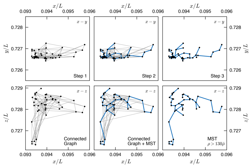
   Figure 14: Algorithm for rapid construction of FOF groups with linking length $b$ from minimum spanning trees. A kD-tree is constructed based on the particle positions, and for each particle the kD-tree is used to search for the nearest $N_{\mathrm{ST}}$ particles. The edges formed by the connections between neighbors are added to a graph. Locally, for each group, these edges form a graph (left column) comprised of the $N_{\mathrm{ST}}$ shortest connections between each vertex and its neighbors. The $x$-$y$ (upper row) and $x$-$z$ (lower row) projections are shown for each graph. The minimum spanning tree (MST) of each graph’s particles is then constructed (blue lines, middle column) using the algorithm of Kruskal (1956). The remaining edges with lengths $l>b$ are then discarded (right column), leaving behind the MST. As a final step, since the algorithm operates on multiple subvolumes of the simulation in parallel MSTs spanning subvolume boundaries are stitched together. The end result is a set of friends-of-friends groups with linking length $b$, each organized into a MST.

3. Construct Minimum Spanning Trees. The use of minimum spanning trees (MSTs) to define FOF groups is a standard technique (see, e.g., Knebe et al., 2011). With a sufficiently large choice for $N_{\mathrm{ST}}$ in the graph construction step, the graph of each dense region will contain the MST of its vertices with edges of lengths $l<b$. The edges comprising the MST are identified using the algorithm of Kruskal (1956). Briefly, starting with the graph of a connected region, edges are added to the tree from shortest to longest. At each insertion, the shortest available edge that does not form a loop in the tree is added. Determining whether adding an edge to the tree would result in a loop amounts to knowing whether the vertices at the ends of the edge already belong to the tree. This issue is complicated somewhat by the Kruskal (1956) algorithm, which effectively involves the merging of subtrees. When constructing the MST, we therefore create a linked list of vertices that belong to a subtree that is “owned” by its densest tracer. Each element in the subtree list contains a pointer to the first element, which in turn tracks the tracer that owns the subtree. When deciding whether to insert an edge, the possible membership of both vertices of the edge can be quickly checked and the insertion vetoed if both vertices are already owned by the same tracer and belong to the same subtree. Otherwise, the subtrees can be merged (with the densest member tracer owning the newly merged tree) or a new subtree created if neither vertex has yet been inserted. The net result of the algorithm is to produce a forest of MSTs that are separated by no less than a distance $b$. This step of the algorithm is illustrated in the middle column of Figure 14.

4. Discard Excess Edges and Retain FOF Groups. The FOF group defined by a linking length $b$ can be constructed from the MST comprised of edges with lengths $l<b$. The algorithm to this point constructs a forest of MSTs whose longest lengths may be $l>b$, so each group is examined and split appropriately by removing any edges that are too long. This step of the algorithm is illustrated in the right column of Figure 14. Again, it should be emphasized that by conditioning the FOF group membership of the tracers on density, distinct regions whose isodensity contours for $\rho\geq\rho_{\mathrm{thresh}}$ do not intersect will remain as separate FOF groups in this algorithm provided the linking length $b$ is not too large. Figure 15 illustrates the relative separation of an example set of FOF groups identified by the algorithm. In this case, the linking length would have to be increased dramatically for these regions to be merged into a single FOF group. The algorithm is therefore expected to be robust to order unity changes in $b$, which we have confirmed in tests.

5. Stitch Subvolumes. The spatial extent of shocked regions varies considerably based on the threshold density $\rho_{\mathrm{thresh}}$, and for a simulation comprised of subvolumes evolved by parallel processes, connected regions may frequently span the boundaries between computational subvolumes. Since the FOF groups are initially constructed for each computational subvolume in parallel, some groups may need to be “stitched” together. For simplicity, this stitching step is performed serially.

6. Repeat with Different Density Thresholds. The group finding algorithm is repeated for a hierarchy of density thresholds, allowing for density enhancements within lower density groups to be identified as distinct local density maxima. If multiple distinct density peaks are identified within a region, lower density particles are assigned to the peak containing the most proximate tracer particle of higher density.

Figure 15 provides an illustration of the above algorithm. The complex density field is apparent in the top panel that shows a logarithmic projection through one-fourth of the volume. The tracer particles moving in response to the fluid properties become concentrated in dense regions (lower right panel). Given an threshold density, in this case $\rho\geq 15\bar{\rho}$, the algorithm groups tracer particles in dense regions into convenient minimum spanning trees (lower left panel). Appendix D describes how these tracer particles groups are used to define interpolation trajectories for measuring the fluid properties near shocks, and Appendix E details how the groups are tracked with time during the simulation.

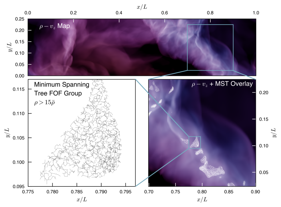
Figure 15: Spatial relation between Friends-of-Friends (FOF) groups and overdense regions in the supersonically turbulent fluid. The fluid is very inhomogeneous, with large variations in the density. The upper panel shows a logarithmic projection of the density field (intensity) through one fourth of the simulation volume, color coded by the $y$-velocity of the fluid (positive velocities are red, negative velocities are blue). Zooming in on a region with large projected density (lower right panel), the filamentary appearance caused by the projection of dense sheets is apparent. The minimum spanning trees comprising the FOF groups (white, constructed for particles with densities $\rho/\bar{\rho}\geq 15$) is overlaid to show regions of large three dimensional density. Zooming in further on a handful of FOF groups (bottom left panel), the distinct character of the dense regions can be seen. The relative separation between groups is considerably larger than their interior mean inter-particle separation.

Appendix D Shock Orientation and Trajectory Interpolation

By selecting tracer particles with densities above some chosen threshold, dense regions in the simulations can be identified and their properties measured. Since regions with densities $\rho\gg\bar{\rho}$ in isothermal turbulence must be generated by shocks, we are interested in measuring the properties around the dense regions in turbulence. Once the dense regions are identified from the tracer particles selected above a given density threshold, their structural properties are estimated from the density distribution probed by the tracers.

To measure a density and relative velocity profile about each shock, an estimate of the local moment of inertia tensor is constructed. For each shocked region, the densest tracer particle is identified. The location of the shocked region peak is taken to be the average position of particles in the tenth percentile of density that are in the closest quintile of particles in separation from the densest tracer. A density-weighted estimate of the moment of inertia tensor is constructed from these $n_{p}$ tracer particles as

$$\mathbf{I}=\frac{1}{\Sigma_{\rho}}\left[\begin{array}[]{ccc}\sum\rho_{i}\left(y_{i}^{2}+z_{i}^{2}\right)&-\sum\rho_{i}x_{i}y_{i}&-\sum\rho_{i}x_{i}z_{i}\\ -\sum\rho_{i}y_{i}x_{i}&\sum\rho_{i}\left(x_{i}^{2}+z_{i}^{2}\right)&-\sum\rho_{i}y_{i}z_{i}\\ -\sum\rho_{i}z_{i}x_{i}&-\sum\rho_{i}z_{i}y_{i}&\sum\rho_{i}\left(x_{i}^{2}+y_{i}^{2}\right)\end{array}\right]$$ (D1)

where $\rho_{i}$, $x_{i}$, $y_{i}$, and $z_{i}$ are the density and $x$, $y$, and $z$ positions of the tracer particles, the summations span the range $i\in[0,n_{p})$ and we abbreviate the sum of the densities as

$$\Sigma_{\rho}=\sum_{i=0}^{n_{p}-1}\rho_{i}.$$ (D2)

The estimated moment of inertia tensor is then diagonalized to find the principal axes of the density distribution near each shocked region peak. We will use $\vec{\xi}$ to denote the eigenvector corresponding to the largest eigenvalue of the moment of inertia tensor. If the dense regions are flattened into sheet-like shocked regions, then we would expect $\vec{\xi}$ to be oriented perpendicular to the shock face. Since the eigenvectors are not uniquely defined to within a reflection, we select the orientation of $\vec{\xi}$ that has a positive projection along the bulk velocity of the shocked region. When tracking the shocked region with time (see below), we choose a consistent orientation of the principal axes.

Once $\vec{\xi}$ is determined, we can parameterize a path through the fluid simulated on the Eulerian grid that runs through the shock parallel to $\vec{\xi}$. In terms of some path length $\eta$, the equation of this line is

$$\vec{x}=x_{0}+\eta\left(\vec{\xi}\cdot\hat{i}\right)\hat{i}$$ (D3)

$$\vec{y}=y_{0}+\eta\left(\vec{\xi}\cdot\hat{j}\right)\hat{j}$$ (D4)

$$\vec{z}=z_{0}+\eta\left(\vec{\xi}\cdot\hat{k}\right)\hat{k},$$ (D5)

where $x_{0}$, $y_{0}$, and $z_{0}$ correspond to the three-dimensional location of the peak about which the moment of inertia tensor is defined. The properties of the fluid along this path near each dense region can be interpolated from the grid for each position $[\vec{x}(\eta),\vec{y}(\eta),\vec{z}(\eta)]$.

Appendix E Shock Tracking Algorithm

Given the methodology for defining shocked regions described in Appendix C, we can engineer a fast parallel scheme for reconstructing the history of shocked regions from a suite of catalogues generated for a sequence of times during the simulation. Assuming the computational domain is divided into adjacent subregions assigned to separate parallel processes, we have found the following simple divide-and-conquer algorithm to work well. Other schemes based on identifying velocity jumps have also been shown to be effective (e.g., Smith et al., 2000a, b).

In our approach, each parallel process compares the shocked regions identified at time $t_{1}$ with shocked regions in the same and adjacent regions at an earlier time $t_{0}$, examining only shocked regions that could have shared particles over the elapsed time $t_{1}-t_{0}$ given their relative velocities. Regions that contain the same particles at different times are incorporated into a recorded history for each region.

Depending on the shock finding algorithm, analogues of the common pathologies seen in dark matter halo merger tree reconstructions (see, e.g., Fakhouri & Ma, 2008) are also encountered in the histories of shocked regions. For instance, since our approach is to use a FOF criterion conditioned on particle density for determining the membership of a tracer particle in a given shocked region, if the topological structure of a shocked region includes a narrow “bridge” the FOF finding algorithm can fragment regions into seemingly unassociated structures at a later or earlier time if the density in the bridge varies with time. Owing to the complicated topology of turbulence, this fragmentation can be physical in origin as the connectivity of isodensity contours can vary over short time scales. As we argued in Appendix C the algorithm is robust to choices in the linking length at any one time, but it is reasonable to expect that derived quantities like the “merging time” of two distinct shocked regions or the possible fragmentation of groups across two time steps will depend on the choice of linking length. Nonetheless, even given these considerations, robust reconstruction of a shocked region’s history can be achieved by either monitoring “ancestor” shocked regions in multiple snapshots at different times simultaneously or, as we prefer, by tracking the histories of all ancestor shocked regions at all previous times and reconstructing the “main branch” of the history after the fact.

With an additional step, the method can also be used to reconstruct the history of fluid surrounding the shocked region and its predecessors. One option is to find all tracers associated with the shocked regions at any time, and then read their properties at all times in the recorded history from the tracer particle snapshot files. A second option is to use the history of the shocked regions to define volumes co-moving with the structures of interest and reconstruct the fluid properties within those volumes from either the tracer particle samples or the Eulerian grid at each time. We have used both these methods for various measurements presented in this work.

References

- André et al. (2010) André, P., Men’shchikov, A., Bontemps, S., et al. 2010, A&A, 518, L102
- Arzoumanian et al. (2011) Arzoumanian, D., André, P., Didelon, P., et al. 2011, A&A, 529, L6
- Ballesteros-Paredes et al. (2006) Ballesteros-Paredes, J., Gazol, A., Kim, J., et al. 2006, ApJ, 637, 384
- Ballesteros-Paredes et al. (1999) Ballesteros-Paredes, J., Hartmann, L., & Vázquez-Semadeni, E. 1999, ApJ, 527, 285
- Ballesteros-Paredes et al. (2011) Ballesteros-Paredes, J., Vázquez-Semadeni, E., Gazol, A., et al. 2011, MNRAS, 416, 1436
- Bate et al. (2003) Bate, M. R., Bonnell, I. A., & Bromm, V. 2003, MNRAS, 339, 577
- Beresnyak (2011) Beresnyak, A. 2011, Physical Review Letters, 106, 075001
- Beresnyak (2014) —. 2014, ApJ, 784, L20
- Bertoldi & McKee (1992) Bertoldi, F., & McKee, C. F. 1992, ApJ, 395, 140
- Bertschinger (2001) Bertschinger, E. 2001, ApJS, 137, 1
- Bigiel et al. (2008) Bigiel, F., Leroy, A., Walter, F., et al. 2008, AJ, 136, 2846
- Blitz & Shu (1980) Blitz, L., & Shu, F. H. 1980, ApJ, 238, 148
- Bolatto et al. (2008) Bolatto, A. D., Leroy, A. K., Rosolowsky, E., Walter, F., & Blitz, L. 2008, ApJ, 686, 948
- Bonnell & Bate (2006) Bonnell, I. A., & Bate, M. R. 2006, MNRAS, 370, 488
- Bonnell et al. (2003) Bonnell, I. A., Bate, M. R., & Vine, S. G. 2003, MNRAS, 343, 413
- Braun & Schmidt (2015) Braun, H., & Schmidt, W. 2015, MNRAS, 454, 1545
- Brunt et al. (2009) Brunt, C. M., Heyer, M. H., & Mac Low, M.-M. 2009, A&A, 504, 883
- Burkhart et al. (2017) Burkhart, B., Stalpes, K., & Collins, D. C. 2017, ApJ, 834, L1
- Caselli & Myers (1995) Caselli, P., & Myers, P. C. 1995, ApJ, 446, 665
- Chen & Ostriker (2014) Chen, C.-Y., & Ostriker, E. C. 2014, ApJ, 785, 69
- Chen et al. (2017) Chen, H., Burkhart, B., Goodman, A. A., & Collins, D. C. 2017, ArXiv e-prints, arXiv:1707.09356
- Cho & Lazarian (2003) Cho, J., & Lazarian, A. 2003, MNRAS, 345, 325
- Colella (1990) Colella, P. 1990, Journal of Computational Physics, 87, 171
- Colella & Woodward (1984) Colella, P., & Woodward, P. R. 1984, Journal of Computational Physics, 54, 174
- Dobbs (2008) Dobbs, C. L. 2008, MNRAS, 391, 844
- Dobbs & Bonnell (2008) Dobbs, C. L., & Bonnell, I. A. 2008, MNRAS, 385, 1893
- Dobbs et al. (2008) Dobbs, C. L., Glover, S. C. O., Clark, P. C., & Klessen, R. S. 2008, MNRAS, 389, 1097
- Dobbs et al. (2015) Dobbs, C. L., Pringle, J. E., & Duarte-Cabral, A. 2015, MNRAS, 446, 3608
- Donkov et al. (2017) Donkov, S., Veltchev, T. V., & Klessen, R. S. 2017, MNRAS, 466, 914
- Elmegreen & Scalo (2004) Elmegreen, B. G., & Scalo, J. 2004, ARA&A, 42, 211
- Evans et al. (2014) Evans, II, N. J., Heiderman, A., & Vutisalchavakul, N. 2014, ApJ, 782, 114
- Fakhouri & Ma (2008) Fakhouri, O., & Ma, C.-P. 2008, MNRAS, 386, 577
- Falgarone et al. (1992) Falgarone, E., Puget, J.-L., & Perault, M. 1992, A&A, 257, 715
- Federrath (2013) Federrath, C. 2013, MNRAS, 436, 1245
- Federrath (2015) —. 2015, MNRAS, 450, 4035
- Federrath (2016) —. 2016, MNRAS, 457, 375
- Federrath & Klessen (2012) Federrath, C., & Klessen, R. S. 2012, ApJ, 761, 156
- Federrath & Klessen (2013) —. 2013, ApJ, 763, 51
- Federrath et al. (2008) Federrath, C., Klessen, R. S., & Schmidt, W. 2008, ApJ, 688, L79
- Federrath et al. (2010) Federrath, C., Roman-Duval, J., Klessen, R. S., Schmidt, W., & Mac Low, M.-M. 2010, A&A, 512, A81
- Fischera (2014a) Fischera, J. 2014a, A&A, 565, A24
- Fischera (2014b) —. 2014b, A&A, 571, A95
- Fischera & Martin (2012) Fischera, J., & Martin, P. G. 2012, A&A, 542, A77
- Fryxell et al. (2000) Fryxell, B., Olson, K., Ricker, P., et al. 2000, ApJS, 131, 273
- Fuller & Myers (1992) Fuller, G. A., & Myers, P. C. 1992, ApJ, 384, 523
- Gao & Solomon (2004) Gao, Y., & Solomon, P. M. 2004, ApJ, 606, 271
- Gardiner & Stone (2008) Gardiner, T. A., & Stone, J. M. 2008, Journal of Computational Physics, 227, 4123
- Genel et al. (2013) Genel, S., Vogelsberger, M., Nelson, D., et al. 2013, MNRAS, 435, 1426
- Ginsburg et al. (2013) Ginsburg, A., Federrath, C., & Darling, J. 2013, ApJ, 779, 50
- Girichidis et al. (2011) Girichidis, P., Federrath, C., Banerjee, R., & Klessen, R. S. 2011, MNRAS, 413, 2741
- Glover & Mac Low (2007a) Glover, S. C. O., & Mac Low, M.-M. 2007a, ApJS, 169, 239
- Glover & Mac Low (2007b) —. 2007b, ApJ, 659, 1317
- Goldreich & Sridhar (1995) Goldreich, P., & Sridhar, S. 1995, ApJ, 438, 763
- Goldreich & Sridhar (1997) —. 1997, ApJ, 485, 680
- Gómez & Vázquez-Semadeni (2014) Gómez, G. C., & Vázquez-Semadeni, E. 2014, ApJ, 791, 124
- Goodman et al. (1998) Goodman, A. A., Barranco, J. A., Wilner, D. J., & Heyer, M. H. 1998, ApJ, 504, 223
- Hartmann et al. (2001) Hartmann, L., Ballesteros-Paredes, J., & Bergin, E. A. 2001, ApJ, 562, 852
- Haugbølle et al. (2017) Haugbølle, T., Padoan, P., & Nordlund, A. 2017, ArXiv e-prints, arXiv:1709.01078
- Heitsch (2013a) Heitsch, F. 2013a, ApJ, 769, 115
- Heitsch (2013b) —. 2013b, ApJ, 776, 62
- Heitsch et al. (2005) Heitsch, F., Burkert, A., Hartmann, L. W., Slyz, A. D., & Devriendt, J. E. G. 2005, ApJ, 633, L113
- Heitsch et al. (2008) Heitsch, F., Hartmann, L. W., & Burkert, A. 2008, ApJ, 683, 786
- Heitsch et al. (2011) Heitsch, F., Naab, T., & Walch, S. 2011, MNRAS, 415, 271
- Heitsch et al. (2009) Heitsch, F., Stone, J. M., & Hartmann, L. W. 2009, ApJ, 695, 248
- Hennebelle & Chabrier (2008) Hennebelle, P., & Chabrier, G. 2008, ApJ, 684, 395
- Hennebelle & Chabrier (2011) —. 2011, ApJ, 743, L29
- Hennebelle & Teyssier (2008) Hennebelle, P., & Teyssier, R. 2008, A&A, 477, 25
- Hennemann et al. (2012) Hennemann, M., Motte, F., Schneider, N., et al. 2012, A&A, 543, L3
- Heyer et al. (2009) Heyer, M., Krawczyk, C., Duval, J., & Jackson, J. M. 2009, ApJ, 699, 1092
- Heyer & Brunt (2004) Heyer, M. H., & Brunt, C. M. 2004, ApJ, 615, L45
- Hockney & Eastwood (1988) Hockney, R. W., & Eastwood, J. W. 1988, Computer simulation using particles (Hilger)
- Hopkins (2013a) Hopkins, P. F. 2013a, MNRAS, 430, 1653
- Hopkins (2013b) —. 2013b, MNRAS, 430, 1880
- Hopkins (2013c) —. 2013c, MNRAS, 428, 1950
- Huchra & Geller (1982) Huchra, J. P., & Geller, M. J. 1982, ApJ, 257, 423
- Ibáñez-Mejía et al. (2016) Ibáñez-Mejía, J. C., Mac Low, M.-M., Klessen, R. S., & Baczynski, C. 2016, ApJ, 824, 41
- Ibáñez-Mejía et al. (2017) —. 2017, ArXiv e-prints, arXiv:1705.01779
- Inoue et al. (2017) Inoue, T., Hennebelle, P., Fukui, Y., et al. 2017, ArXiv e-prints, arXiv:1707.02035
- Kainulainen et al. (2009) Kainulainen, J., Beuther, H., Henning, T., & Plume, R. 2009, A&A, 508, L35
- Kainulainen et al. (2014) Kainulainen, J., Federrath, C., & Henning, T. 2014, Science, 344, 183
- Kennicutt & Evans (2012) Kennicutt, R. C., & Evans, N. J. 2012, ARA&A, 50, 531
- Kim et al. (2006) Kim, C.-G., Kim, W.-T., & Ostriker, E. C. 2006, ApJ, 649, L13
- Kim et al. (2008) —. 2008, ApJ, 681, 1148
- Kirk et al. (2013) Kirk, H., Myers, P. C., Bourke, T. L., et al. 2013, ApJ, 766, 115
- Klessen (2001) Klessen, R. S. 2001, ApJ, 556, 837
- Klessen et al. (1998) Klessen, R. S., Burkert, A., & Bate, M. R. 1998, ApJ, 501, L205
- Klessen et al. (2000) Klessen, R. S., Heitsch, F., & Mac Low, M.-M. 2000, ApJ, 535, 887
- Knebe et al. (2011) Knebe, A., Knollmann, S. R., Muldrew, S. I., et al. 2011, MNRAS, 415, 2293
- Kolmogorov (1941) Kolmogorov, A. 1941, Akademiia Nauk SSSR Doklady, 30, 301
- Konstandin et al. (2012) Konstandin, L., Girichidis, P., Federrath, C., & Klessen, R. S. 2012, ApJ, 761, 149
- Könyves et al. (2015) Könyves, V., André, P., Men’shchikov, A., et al. 2015, A&A, 584, A91
- Körtgen & Banerjee (2015) Körtgen, B., & Banerjee, R. 2015, MNRAS, 451, 3340
- Körtgen et al. (2017) Körtgen, B., Federrath, C., & Banerjee, R. 2017, ArXiv e-prints, arXiv:1703.07232
- Kraichnan (1959) Kraichnan, R. H. 1959, Journal of Fluid Mechanics, 5, 497
- Kritsuk et al. (2007) Kritsuk, A. G., Norman, M. L., Padoan, P., & Wagner, R. 2007, ApJ, 665, 416
- Kritsuk et al. (2011) Kritsuk, A. G., Norman, M. L., & Wagner, R. 2011, ApJ, 727, L20
- Krumholz (2014) Krumholz, M. R. 2014, Phys. Rep., 539, 49
- Krumholz et al. (2012) Krumholz, M. R., Dekel, A., & McKee, C. F. 2012, ApJ, 745, 69
- Krumholz & McKee (2005) Krumholz, M. R., & McKee, C. F. 2005, ApJ, 630, 250
- Krumholz & Tan (2007) Krumholz, M. R., & Tan, J. C. 2007, ApJ, 654, 304
- Kruskal (1956) Kruskal, J. B. 1956, Proc. American Math. Soc., 7, 48
- Lada et al. (2012) Lada, C. J., Forbrich, J., Lombardi, M., & Alves, J. F. 2012, ApJ, 745, 190
- Lada et al. (2017) Lada, C. J., Lewis, J. A., Lombardi, M., & Alves, J. 2017, ArXiv e-prints, arXiv:1708.07847
- Lada et al. (2010) Lada, C. J., Lombardi, M., & Alves, J. F. 2010, ApJ, 724, 687
- Lada et al. (2013) Lada, C. J., Lombardi, M., Roman-Zuniga, C., Forbrich, J., & Alves, J. F. 2013, ApJ, 778, 133
- Landy & Szalay (1993) Landy, S. D., & Szalay, A. S. 1993, ApJ, 412, 64
- Larson (1981) Larson, R. B. 1981, MNRAS, 194, 809
- Lee et al. (2015) Lee, E. J., Chang, P., & Murray, N. 2015, ApJ, 800, 49
- Lemaster & Stone (2008) Lemaster, M. N., & Stone, J. M. 2008, ApJ, 682, L97
- Li et al. (2017) Li, P. S., Klein, R. I., & McKee, C. F. 2017, ArXiv e-prints, arXiv:1708.06770
- Li et al. (2003) Li, Y., Klessen, R. S., & Mac Low, M.-M. 2003, ApJ, 592, 975
- Liptai et al. (2017) Liptai, D., Price, D. J., Wurster, J., & Bate, M. R. 2017, MNRAS, 465, 105
- Mac Low (1999) Mac Low, M.-M. 1999, ApJ, 524, 169
- Mac Low & Klessen (2004) Mac Low, M.-M., & Klessen, R. S. 2004, Reviews of Modern Physics, 76, 125
- Mac Low et al. (1998) Mac Low, M.-M., Klessen, R. S., Burkert, A., & Smith, M. D. 1998, Physical Review Letters, 80, 2754
- Matzner & McKee (2000) Matzner, C. D., & McKee, C. F. 2000, ApJ, 545, 364
- McKee & Ostriker (2007) McKee, C. F., & Ostriker, E. C. 2007, ARA&A, 45, 565
- McKee & Tan (2003) McKee, C. F., & Tan, J. C. 2003, ApJ, 585, 850
- Men’shchikov et al. (2010) Men’shchikov, A., André, P., Didelon, P., et al. 2010, A&A, 518, L103
- Miville-Deschênes et al. (2010) Miville-Deschênes, M.-A., Martin, P. G., Abergel, A., et al. 2010, A&A, 518, L104
- Mo & White (1996) Mo, H. J., & White, S. D. M. 1996, MNRAS, 282, 347
- Mocz et al. (2017) Mocz, P., Burkhart, B., Hernquist, L., McKee, C. F., & Springel, V. 2017, ApJ, 838, 40
- Moeckel & Burkert (2015) Moeckel, N., & Burkert, A. 2015, ApJ, 807, 67
- Molina et al. (2012) Molina, F. Z., Glover, S. C. O., Federrath, C., & Klessen, R. S. 2012, MNRAS, 423, 2680
- More et al. (2011) More, S., Kravtsov, A. V., Dalal, N., & Gottlöber, S. 2011, ApJS, 195, 4
- Murray et al. (2017) Murray, D. W., Chang, P., Murray, N. W., & Pittman, J. 2017, MNRAS, 465, 1316
- Murray (2011) Murray, N. 2011, ApJ, 729, 133
- Murray & Chang (2015) Murray, N., & Chang, P. 2015, ApJ, 804, 44
- Myers (1983) Myers, P. C. 1983, ApJ, 270, 105
- Myers (2015) —. 2015, ApJ, 806, 226
- Offner et al. (2008) Offner, S. S. R., Klein, R. I., & McKee, C. F. 2008, ApJ, 686, 1174
- Ostriker et al. (2001) Ostriker, E. C., Stone, J. M., & Gammie, C. F. 2001, ApJ, 546, 980
- Padoan et al. (2017) Padoan, P., Haugbølle, T., Nordlund, Å., & Frimann, S. 2017, ApJ, 840, 48
- Padoan & Nordlund (2002) Padoan, P., & Nordlund, Å. 2002, ApJ, 576, 870
- Padoan & Nordlund (2011) —. 2011, ApJ, 730, 40
- Padoan et al. (1997) Padoan, P., Nordlund, A., & Jones, B. J. T. 1997, MNRAS, 288, 145
- Passot & Vázquez-Semadeni (1998) Passot, T., & Vázquez-Semadeni, E. 1998, Phys. Rev. E, 58, 4501
- Pavlovski et al. (2006) Pavlovski, G., Smith, M. D., & Mac Low, M.-M. 2006, MNRAS, 368, 943
- Perez et al. (2012) Perez, J. C., Mason, J., Boldyrev, S., & Cattaneo, F. 2012, Physical Review X, 2, 041005
- Plume et al. (1997) Plume, R., Jaffe, D. T., Evans, II, N. J., Martín-Pintado, J., & Gómez-González, J. 1997, ApJ, 476, 730
- Price et al. (2011) Price, D. J., Federrath, C., & Brunt, C. M. 2011, ApJ, 727, L21
- Raskutti et al. (2016) Raskutti, S., Ostriker, E. C., & Skinner, M. A. 2016, ApJ, 829, 130
- Rasmussen & Williams (2006) Rasmussen, C. E., & Williams, C. K. I. 2006, Gaussian Processes for Machine Learning (The MIT Press)
- Reyes et al. (2016) Reyes, A., Lee, D., Graziani, C., & Tzeferacos, P. 2016, ArXiv e-prints, arXiv:1611.08084 [physics.comp-ph]
- Robertson & Goldreich (2012) Robertson, B., & Goldreich, P. 2012, ApJ, 750, L31
- Roman-Duval et al. (2010) Roman-Duval, J., Jackson, J. M., Heyer, M., Rathborne, J., & Simon, R. 2010, ApJ, 723, 492
- Rosen et al. (2016) Rosen, A. L., Krumholz, M. R., McKee, C. F., & Klein, R. I. 2016, MNRAS, 463, 2553
- Rycroft (2009) Rycroft, C. H. 2009, Chaos, 19, 041111
- Scalo et al. (1998) Scalo, J., Vazquez-Semadeni, E., Chappell, D., & Passot, T. 1998, ApJ, 504, 835
- Scalo & Pumphrey (1982) Scalo, J. M., & Pumphrey, W. A. 1982, ApJ, 258, L29
- Schneider et al. (2011) Schneider, N., Bontemps, S., Simon, R., et al. 2011, A&A, 529, A1
- Schneider et al. (2012) Schneider, N., Csengeri, T., Hennemann, M., et al. 2012, A&A, 540, L11
- Semenov et al. (2016) Semenov, V. A., Kravtsov, A. V., & Gnedin, N. Y. 2016, ApJ, 826, 200
- Sheth & Tormen (1999) Sheth, R. K., & Tormen, G. 1999, MNRAS, 308, 119
- Shu (1991) Shu, F. H. 1991, The Physics of Astrophysics: Gas Dynamics, Vol. 2 (University Science Books)
- Shu et al. (1973) Shu, F. H., Milione, V., & Roberts, Jr., W. W. 1973, ApJ, 183, 819
- Smith et al. (2000a) Smith, M. D., Mac Low, M.-M., & Heitsch, F. 2000a, A&A, 362, 333
- Smith et al. (2000b) Smith, M. D., Mac Low, M.-M., & Zuev, J. M. 2000b, A&A, 356, 287
- Smith et al. (2014) Smith, R. J., Glover, S. C. O., & Klessen, R. S. 2014, MNRAS, 445, 2900
- Smith et al. (2016) Smith, R. J., Glover, S. C. O., Klessen, R. S., & Fuller, G. A. 2016, MNRAS, 455, 3640
- Solomon et al. (1987) Solomon, P. M., Rivolo, A. R., Barrett, J., & Yahil, A. 1987, ApJ, 319, 730
- Stone et al. (2008) Stone, J. M., Gardiner, T. A., Teuben, P., Hawley, J. F., & Simon, J. B. 2008, ApJS, 178, 137
- Stone et al. (1998) Stone, J. M., Ostriker, E. C., & Gammie, C. F. 1998, ApJ, 508, L99
- Stutzki et al. (1998) Stutzki, J., Bensch, F., Heithausen, A., Ossenkopf, V., & Zielinsky, M. 1998, A&A, 336, 697
- Tasker & Tan (2009) Tasker, E. J., & Tan, J. C. 2009, ApJ, 700, 358
- Tinker et al. (2010) Tinker, J. L., Robertson, B. E., Kravtsov, A. V., et al. 2010, ApJ, 724, 878
- Towns et al. (2014) Towns, J., Cockerill, T., Dahan, M., et al. 2014, Computing in Science & Engineering, 16, 62
- Vazquez-Semadeni (1994) Vazquez-Semadeni, E. 1994, ApJ, 423, 681
- Vázquez-Semadeni et al. (2003) Vázquez-Semadeni, E., Ballesteros-Paredes, J., & Klessen, R. S. 2003, ApJ, 585, L131
- Vázquez-Semadeni et al. (2005) Vázquez-Semadeni, E., Kim, J., Shadmehri, M., & Ballesteros-Paredes, J. 2005, ApJ, 618, 344
- Vázquez-Semadeni et al. (2006) Vázquez-Semadeni, E., Ryu, D., Passot, T., González, R. F., & Gazol, A. 2006, ApJ, 643, 245
- Veltchev et al. (2016) Veltchev, T. V., Donkov, S., & Klessen, R. S. 2016, MNRAS, 459, 2432
- Vishniac (1994) Vishniac, E. T. 1994, ApJ, 428, 186