Two-Stage LASSO ADMM Signal Detection Algorithm For Large Scale MIMO

Abstract

This paper explores the benefit of using some of the machine learning techniques and Big data optimization tools in approximating maximum likelihood (ML) detection of Large Scale MIMO systems. First, large scale MIMO detection problem is formulated as a LASSO (Least Absolute Shrinkage and Selection Operator) optimization problem. Then, Alternating Direction Method of Multipliers (ADMM) is considered in solving this problem. The choice of ADMM is motivated by its ability of solving convex optimization problems by breaking them into smaller sub-problems, each of which are then easier to handle. Further improvement is obtained using two stages of LASSO with interference cancellation from the first stage. The proposed algorithm is investigated at various modulation techniques with different number of antennas. It is also compared with widely used algorithms in this field. Simulation results demonstrate the efficacy of the proposed algorithm for both uncoded and coded cases.

I Introduction

Large scale Multi Input Multi Output antennas (MIMO) is a key technology for various wireless systems, because of its numerous advantages in providing high capacity and signal quality [1]. It has applications for both single user and multi user wireless systems, however, a single user MIMO with a large number of antennas at both sides of the wireless link gained more interest nowadays, especially in the next generation 5G wireless backhaul links [2].
The challenges in presenting large scale MIMO signal detection algorithms depend on how to achieve good quality in terms of bit error performance simultaneously with low complexity at various modulation orders. Several techniques have been proposed in the literature to address these challenges. One group of algorithms that is based on the neighborhood search technique, such as the family of Likelihood Ascent Search (LAS) [3], [4] and Reactive Tabu Search (RTS) [5], [6], [7]. These algorithms have advantages mainly at low modulation orders, such as QPSK, however their performance and complexity deteriorates at higher modulations and higher number of antennas [8]. Another group of algorithms that are based on semidefinite programming (SDP), such as Quadratic Programming and Branch and Bound [8]. In addition to other algorithms that use believe propagation ideas [9].
In this paper, we formulate ML problem into least absolute shrinkage and selection operator (LASSO) optimization problem [10]. The success of LASSO in performing high dimensional data clustering and classification [11] motivated us to cast the problem of the large-scale MIMO detection into the domain of data classification. Among many useful features, one key feature of the this formulation is that its modular structure which allows one to sparsely represent any received signal as a linear combination of the modulated symbols.

LASSO is a convex optimization problem which can be solved using any generic convex solver. However, we choose to use alternating direction method of multipliers (ADMM) because it takes the advantage of the separability of the LASSO objective function and makes the variable updates in every iteration much easier. That’s, at every iteration, each variable is updated in a closed form expression by solving an unconstrained strong convex optimization problem. ADMM is a widely used algorithm for solving separable convex optimization problems with linear constraints. Its global convergence was established in the early 1990’s by Eckstein and Bertsekas [12]. The interest in ADMM has exploded in recent years because of applications in signal and image processing, compressed sensing [13], distributed optimization, statistical machine learning [14], and quadratic and linear programming [15].
We further improve LASSO ADMM detection by implementing two stages LASSO optimization for better performance, which will be denoted in this paper as (2 LASSO ADMM). The idea is to implement the second stage of LASSO ADMM detection based on interference cancellation from the first stage. This improves the detection performance significantly. The simulation experiments show the efficacy of the proposed algorithm in both coded and uncoded performance at various QAM modulations.
The remainder of this paper is organized as follows. In Section II, system model is discribed. Section III contains problem formulation, and section IV presents proposed algorithm. Finally, simulation results and conlusion are provided.

II System Model

We consider a MIMO system with $N_{t}$ transmit antennas and $N_{r}$ receive antennas employing a spatial multiplexing (V-BLAST) transmission. At the transmitter side, the source information is generated and then mapped to symbols of different alphabet. The mapped complex symbols are demultiplexed into $N_{t}$ separate independent data streams with a transmitted signal vector $\tilde{\textbf{x}}=[{\tilde{x}}_{1},\dots,{\tilde{x}}_{N_{t}}]^{T}\in\mathbb{C}^{N_{t}\times 1}$. The general MIMO channel model is :

$$\tilde{\textbf{{y}}}=\tilde{\textbf{{H}}}\tilde{\textbf{{x}}}+\tilde{\textbf{{n}}}$$ (1)

where ${\tilde{\textbf{y}}}=[{\tilde{y}}_{1},\dots,{\tilde{y}}_{N_{r}}]^{T}\in\mathbb{C}^{N_{r}\times 1}$ is the received signal vector at all $N_{r}$ antennas, $\tilde{\textbf{H}}\in\mathbb{C}^{N_{r}\times N_{t}}$ denotes the flat fading channel gain matrix whose entries are modeled as $\mathbb{C}\mathcal{N}(0,1)$, and $\tilde{\textbf{{n}}}$ represents the receiver AWGN noise vector whose entries are modeled as i.i.d $\mathbb{C}\mathcal{N}(0,\sigma^{2})$. The tilde symbol in (1) is made to distinguish the complex model from the real model. We assume ideal channel estimation and synchronization at the receiver end. The ML problem of model (1), which is equivalent to Euclidean distance minimization, can be expressed as:

$$\widehat{\widetilde{\textbf{{x}}}}=\underset{{{{\widetilde{{\textbf{x}}}}}\in\widetilde{\chi}^{N_{t}}}}{\text{argmin}}\parallel{\widetilde{\textbf{y}}-\widetilde{\textbf{{H}}\,}\widetilde{\textbf{{x}}}\parallel_{2}^{2}}$$ (2)

where $\tilde{\chi}^{N_{t}}\normalsize$ is the set of all possible $N_{t}$-dimensional complex candidate vectors of the transmitted vector $\tilde{\textbf{{x}}}$. The equivalent real system model of (1) is:

$$\vspace{-.05in}\textbf{{y}}=\textbf{{H}}\textbf{{x}}+\textbf{{v}}\vspace{-.00in}$$ (3)

$${\textbf{{y}}}=\begin{array}[]{c}\begin{bmatrix}\Re\{{\tilde{\textbf{{y}}}}\}\\ \Im\{{\tilde{\textbf{{y}}}}\}\end{bmatrix}\end{array},\textbf{{x}}=\begin{array}[]{c}\begin{bmatrix}\Re\{{{\tilde{\textbf{{x}}}}}\}\\ \Im\{{{\tilde{\textbf{{x}}}}}\}\end{bmatrix}\end{array},\textbf{{n}}=\begin{array}[]{c}\begin{bmatrix}\Re\{{{\tilde{\textbf{{n}}}}}\}\\ \Im\{{{\tilde{\textbf{{n}}}}}\}\end{bmatrix}\end{array}\\$$ (4)

$$\mathbf{{H}}=\begin{bmatrix}\Re\{\tilde{\textbf{{H}}}\}&-\Im\{\tilde{\textbf{{H}}}\}\\ \Im\{\tilde{\textbf{{H}}}\}&\Re\{\tilde{\textbf{{H}}}\}\end{bmatrix}$$ (5)

In this real-valued system model, the real part of the complex data symbols is mapped to $[x_{1},\dots,x_{Nt}]$ and the imaginary part of these symbols is mapped to $[x_{Nt+1},\dots,x_{2Nt}]$. Now, the equivalent ML detection problem of the real model is :

$$\widehat{{\textbf{x}}}=\underset{{{\textbf{x}}\in\chi^{2N_{t}}}}{\text{argmin}}\parallel{{\textbf{y}}}-{{\textbf{H}}}{{\textbf{x}}}\parallel_{2}^{2}$$ (6)

where set $\chi=\{-\sqrt{\textit{M}}+1,..,-1,1,...,\sqrt{\textit{M}}-1\}$, and M is the QAM constellation size.

III Problem Formulation

To introduce our formulation, we first start by representing each symbol in the transmitted vector x as a sparse linear combination of the elements in $\chi$. To illustrate, if the constellation size is $M$, there will be $m=\sqrt{M}$ elements, $s_{1},s_{2},....,s_{m}$. Hence, x can be expressed as

x $$=\boldsymbol{S}\boldsymbol{\alpha}\vspace{-2.25in}$$ (7)

where

$\!\!\boldsymbol{S\!=}\!\left(\!\!\begin{array}[]{cccccccccc}s_{1}&\ldots&s_{m}&0&\ldots&&&&&0\\ 0&\ldots&0&s_{1}&\ldots&s_{m}&0&&&0\\ \vdots\!&&\!&&\!&&\ddots\\ &&&&&&&\ddots\\ 0&\ldots&\ldots&\ldots&&&&s_{1}&\ldots&s_{m}\end{array}\!\!\right)$

and,
$\boldsymbol{\alpha=}\left(\begin{array}[]{cccccccc}\alpha_{1}&\ldots&\alpha_{m}&\alpha_{m+1}&\ldots&\alpha_{2m+1}&\ldots&\alpha_{N_{t}m}\end{array}\right)^{T}$

Note that the first transmitted symbol is expressed as follows:

$$\textbf{x}(1)=s_{1}\alpha_{1}+s_{2}\alpha_{2}+\ldots+s_{n}\alpha_{n}+\ldots+s_{m}\alpha_{m}.$$ (8)

Similarly, the second symbol can be written as

$$\textbf{x}(2)=s_{1}\alpha_{(m+1)}+s_{2}\alpha_{(m+2)}+\ldots+s_{m}\alpha_{2m}.$$ (9)

In general, the $i$th symbol can be expressed as

$$\textbf{x}(i)=s_{1}\alpha_{((i-1)m+1)}+s_{2}\alpha_{((i-1)m+2)}+\ldots+s_{m}\alpha_{im}$$ (10)

We denote the coefficients of the element x(i) $\{\alpha_{((i-1)m)},.....\alpha_{im}\}\in\boldsymbol{\alpha}$ by ${\boldsymbol{\alpha}_{x}}_{i}$. Typically, if $\textbf{x}(i)=s_{n}$, then the only non zero element $\in{\boldsymbol{\alpha}_{x}}_{i}$ is $\alpha_{(i-1)m+n}$, and its value is exactly one. Therefore, the following holds true

$$\vspace{-.10in}\sum_{j=(i-1)m}^{im}\alpha_{j}=1,\forall i\vspace{-.00in}$$ (11)

We can write (11) in a matrix form as follow

$$\boldsymbol{B}\boldsymbol{\alpha}=\boldsymbol{1}$$ (12)

where

$$\boldsymbol{B=}\left(\begin{array}[]{cccccccccc}1&\ldots&1&0&\ldots&&&&&0\\ 0&\ldots&0&1&\ldots&1&0&&&0\\ \vdots&&&&&&\ddots\\ &&&&&&&\ddots\\ 0&\ldots&\ldots&\ldots&&&&1&\ldots&1\end{array}\right)$$

Next, we explain our MIMO detection optimization framework. Mathematically, we formulate our constrained optimization problem as follows:

$$\begin{array}[]{cc}\widehat{\textbf{x}}=\underset{\text{$\textbf{x}\in$}\mathbb{R}^{mN_{t}}}{\text{argmin}}&\left(\left\|\boldsymbol{\boldsymbol{\textbf{y}-\text{{H}{x}}}}\right\|_{2}^{2}+\lambda\left\|\boldsymbol{\alpha}\right\|_{0}\right)\\ \text{subject to}\\ &\boldsymbol{\text{$\textbf{x}$-}\boldsymbol{S}\alpha=0}\\ &\boldsymbol{\boldsymbol{B}}\boldsymbol{\alpha}=1\end{array}$$ (13)

In (13), the constraint of the non convexity of the feasible set on x is relaxed, but norm zero in the objective function and the two constraints are introduced to approximate the solution of the problem given in (6) if $\lambda$ is chosen carefully.

However, the formulation in (13) has two issues. First, minimizing the zero norm is a well known NP hard problem. Second, compared to problem (6) another variable ($\alpha$) is introduced which increases the number of optimized variables.

In order to solve the first issue, we replace norm zero by norm one (convex relaxation of norm 0), hence the problem becomes convex. Moreover, the second issue can be easily resolved by expressing x in terms of $\boldsymbol{\alpha}$ and that will further cancel the first constraint. so, (13) reduces to:

$$\hat{{\boldsymbol{\alpha}}}=\underset{{{\boldsymbol{\alpha}}}}{\text{argmin}}\bigg{(}\frac{1}{2}\parallel{{\textbf{y}}}-{\widetilde{\textbf{H}}}{{\boldsymbol{\alpha}}}\parallel_{2}^{2}+\lambda^{\prime}||\boldsymbol{\alpha}||_{1}\bigg{)}$$ (14)

subject to

$$\textbf{B}\boldsymbol{\alpha}=\textbf{1}.$$

where $\widetilde{\textbf{H}}=\textbf{H\,S}$, and $\lambda^{\prime}=\frac{\lambda}{2}$. Note that (14) is constrained LASSO. However, since the constraint in (14) can tolerate some violation, it can be expressed as non-constrained optimization problem as follows:

$$\hat{{\boldsymbol{\alpha}}}=\underset{{{\boldsymbol{\alpha}}}}{\text{argmin}}\bigg{(}\frac{1}{2}\parallel{{\textbf{y}}}-{{\textbf{$\widetilde{\boldsymbol{H}}$}}}{{\boldsymbol{\alpha}}}\parallel_{2}^{2}+\mu\parallel{{\textbf{1}}}-{{\textbf{B}}}{{\boldsymbol{\alpha}}}\parallel_{2}^{2}+\lambda^{\prime}||\boldsymbol{\alpha}||_{1}\bigg{)}.$$ (15)

We choose $\mu$ such that $\mu\gg\text{max}(\frac{1}{2},\lambda^{\prime})$ to prioritize reducing the constraint violation over fitting the quadratic term and norm one minimization. Finally, (15) can be re-written in the standard LASSO form as follow as follows:

$$\widehat{\boldsymbol{\alpha}}=\underset{\boldsymbol{\alpha}}{\text{argmin}}\bigg{(}\frac{1}{2}\parallel\overline{\textbf{y}}-\overline{\textbf{H}}\,\boldsymbol{\alpha}\parallel_{2}^{2}+\lambda^{\prime}||\boldsymbol{\alpha}||_{1}\bigg{)}$$ (16)

where

$\overline{\textbf{y}}=\begin{bmatrix}\textbf{y}\\ \sqrt{\mu}\,\textbf{1}\end{bmatrix}$, and $\overline{\textbf{H}}=\begin{bmatrix}\textbf{$\widetilde{\boldsymbol{H}}$}\\ \sqrt{\mu}\,\textbf{B}\end{bmatrix}$

Next, we present our ADMM based algorithm to solve this problem efficiently.

IV Proposed Algorithm

IV-A LASSO-ADMM

To find the coefficients vector ($\boldsymbol{\alpha}$), we solve (16) using ADMM framework described in Algorithm 1. ADMM convergence is proven for any problem with an objective function that is sum of two separable convex functions with linear constraints. Hence, we re-formulate LASSO as a sum of two separable convex functions with a linear constraint as follows:

$$\underset{{{\boldsymbol{\alpha},\textbf{z}}}}{\text{min}}\bigg{(}\frac{1}{2}\parallel{\overline{\textbf{y}}}-\overline{{\textbf{H}}}{{\boldsymbol{\alpha}}}\parallel_{2}^{2}+\lambda^{\prime}||\textbf{z}||_{1}\bigg{)}$$ (17)

subject to

$$\boldsymbol{\alpha}=\textbf{z}$$ (18)

Note that the constrained optimization problem (17-18) is equivalent to (16)

The augmented Lagrangian for (17)-(18) is:

$$\mathcal{\boldsymbol{\mathcal{L}}}_{\rho}\left(\boldsymbol{\alpha},\,{\textbf{z}},\,\boldsymbol{\eta}\right) =\frac{1}{2}\parallel\overline{\textbf{y}}-\overline{\textbf{H}}\boldsymbol{\alpha}\parallel_{2}^{2}+\lambda^{\prime}||{\textbf{z}}||_{1}+\boldsymbol{\eta}^{T}\left(\boldsymbol{\alpha}-{\textbf{z}}\right)$$

$$\,\,\,\,\,\,\,\,+\frac{\rho}{2}\parallel\boldsymbol{\alpha}-{\textbf{z}}\parallel_{2}^{2}$$ (19)

At the $(k+1)$th iteration, the primal ($\boldsymbol{\alpha},{\bf z}$) and dual ($\boldsymbol{\eta}$) variables are updated sequentially as follows:

$$\boldsymbol{\alpha}^{k+1} =\underset{\boldsymbol{\alpha}}{\text{argmin}}\mathcal{\boldsymbol{\mathcal{L}}}_{\rho}\left(\boldsymbol{\alpha},\,{\textbf{z}}^{k},\,\boldsymbol{\eta}^{k}\right)$$ (20)

$$\boldsymbol{\textbf{z}}^{k+1} =\underset{{\textbf{z}}}{\text{argmin}}\mathcal{\boldsymbol{\mathcal{L}}}_{\rho}\left(\boldsymbol{\alpha}^{k+1},\,{\textbf{z}},\,\boldsymbol{\eta}^{k}\right)$$ (21)

$$\boldsymbol{\eta}^{k+1} =\boldsymbol{\eta}^{k}+\left(\boldsymbol{\alpha}^{k+1}-{\textbf{z}}^{k+1}\right)$$ (22)

The primal variables ($\boldsymbol{\alpha}$, z) are updated as follows:

• $\boldsymbol{\alpha}$-update:

  $$\boldsymbol{\alpha}^{k+1}=\underset{\boldsymbol{\alpha}}{\text{argmin}}\bigg{(}\frac{1}{2}\parallel\overline{\textbf{y}}-\overline{\textbf{H}}\boldsymbol{\alpha}\parallel_{2}^{2}+\left(\boldsymbol{\eta}^{k}\right)^{T}\boldsymbol{\alpha}+\frac{\rho}{2}\parallel\boldsymbol{\alpha}-{\textbf{z}}\parallel_{2}^{2}\bigg{)}$$ (23)

  Since (23) is strictly convex with respect to $\boldsymbol{\alpha}$, taking the derivative and equating to zero yields a closed form expression for obtaining $\boldsymbol{\alpha}^{k+1}$.

• z-update:

  $${\textbf{z}}^{k+1}=\underset{\textbf{z}}{\text{argmin}}\bigg{(}\lambda^{\prime}||{\textbf{z}}||_{1}-\left(\boldsymbol{\eta}^{k}\right)^{T}{\textbf{z}}+\frac{\rho}{2}\parallel\boldsymbol{\alpha}^{k+1}-{\textbf{z}}\parallel_{2}^{2}\bigg{)}$$ (24)

  Since the minimized function in (24) is separable with respect to every element in z, it can be written as a sum of independent terms:

  $$f(\boldsymbol{\alpha}^{k+1},\textbf{z},\boldsymbol{\eta}^{k})=\sum_{i=1}^{N}\Big{(}\frac{\rho}{2}(\textbf{$\boldsymbol{\alpha}$}_{i}^{k+1}-\textbf{z}_{i})^{2}+\lambda^{\prime}|\textbf{z}_{i}|-{\eta^{k}}_{i}\textbf{z}_{i}\Big{)}$$ (25)

  For each element, $\textbf{z}_{i}^{k+1}$, the solution can therefore be computed by independently minimizing $f(\boldsymbol{\alpha}^{k+1},\textbf{z},\boldsymbol{\eta}^{k})$ with respect to that element. Moreover, all elements can be updated in parallel. Hence, the $i$th element update is defined by the following equation:

  $$\underset{{\textbf{z}_{i}}}{\text{argmin}}\left\{\begin{array}[]{l}\frac{\rho}{2}(\textbf{$\alpha$}_{i}^{k+1}-\textbf{z}_{i})^{2}+\lambda^{\prime}|\textbf{z}_{i}|-{\eta}_{i}^{k}\textbf{z}_{i}\end{array}\right\}=$$ (27)

  $$\begin{cases}\begin{array}[]{l}\frac{1}{\rho}(\rho(\alpha_{i}^{k+1}+\eta_{i}^{k})-\lambda^{\prime}),\end{array}&\rho(\alpha_{i}^{k+1}+\eta_{i}^{k})>\lambda^{\prime}\\ 0&|\rho(\alpha_{i}^{k+1}+\eta_{i}^{k})|\leq\lambda^{\prime}\\ \frac{1}{\rho}(\rho(\alpha_{i}^{k+1}+\eta_{i}^{k})+\lambda^{\prime})&\rho(\alpha_{i}^{k+1}+\eta_{i}^{k})<-\lambda^{\prime}\end{cases}$$ (28)

After the coefficients ($\boldsymbol{\alpha}$ vector) are found, the received vector x can be found, $\textbf{x}=\boldsymbol{S\alpha}$. Further, since ${\boldsymbol{\alpha_{x}}}_{i}$ may not be sparse for every $\textbf{x}(i)$, $\textbf{x}(i)$ is quantized to the nearest symbol in the constellation set $\chi$, (lines 10-12). The quantization function is defined by $\boldsymbol{Q}(\textbf{x}(i),\chi)$.

1:  1: Initilization

2:  $(\boldsymbol{\bf\alpha}^{0},\textbf{z}^{0},\boldsymbol{\bf\eta}^{0})\leftarrow(\textbf{0,0,0})$

3:  $k=1$

4:  2: ADMM iteration:

5:  while (1) do

6:     $\boldsymbol{\alpha}^{k}\leftarrow\underset{\boldsymbol{\alpha}}{\text{argmin}}\mathcal{L}_{\rho}(\textbf{$\boldsymbol{\alpha}$},\textbf{z}^{k-1},\textbf{$\boldsymbol{\eta}$}^{k-1})$

7:     $\boldsymbol{z}^{k}\leftarrow\underset{\boldsymbol{z}}{\text{argmin}}\mathcal{L}_{\rho}(\textbf{$\boldsymbol{\alpha}^{k}$},\textbf{z},\textbf{$\boldsymbol{\eta}$}^{k-1})$

8:     $\boldsymbol{\eta}^{k}\leftarrow\boldsymbol{\eta}^{k-1}+(\boldsymbol{\alpha}^{k}-\textbf{z}^{k})$

9:     if $||\boldsymbol{\eta}^{k}-\boldsymbol{\eta}^{k-1}||<\epsilon$ then

10:        break

11:     end if

12:     $k=k+1$

13:  end while

14:  $\textbf{x}=\boldsymbol{S\,\alpha}$

15:  for $i=1:2N_{t}$ do

16:     $\hat{\textbf{x}}(i)=\boldsymbol{Q}(\textbf{x}(i),\chi)$

17:  end for

Algorithm 1 LASSO-ADMM Algorithm

IV-B Two-LASSO-ADMM

The idea of this algorithm (Algorithm 2) is to implement two stages of the LASSO detection with interference cancellation to further improve the detection of the unreliable symbols. The main difference compared to LASSO, is that after the first shot of LASSO, the estimate of the received vector x is found, and the line (decision region) between any two modulated symbols ($s_{l}$, and $s_{h}$) is split into three regimes. Any element in the received vector $\textbf{x}(i)$ falls within a predefined threshold ($\tau$) from either $s_{l}$ or $s_{r}$ is rounded to that point. However, any point falls between these two points but it is not within $\tau$ distance from any of them (gray zone) is not rounded to any of the symbols, and it is referred to the second stage of the detection algorithm(lines 16-27 Algorithm 2). Therefore, some of the received symbols are detected from the first round, but some others are deferred to the second round (not yet detected). For any symbol $\textbf{x}(i)$ that is detected from the first round, its corresponding coefficients are found (${\boldsymbol{\alpha}_{x}}_{i}$), so they are excluded (removed) from the second round along with their contribution in $\overline{\textbf{y}}$ and corresponding columns in the matrices B and S (those columns denoted by ${{I_{\alpha}}_{x}}_{i}$. At the second LASSO round, every detected symbol ($\textbf{x}(i)$) is quantized to the nearest symbol in the constellation set $\chi$.

We conclude this section by pointing out that the main ingredient in the computations of the LASSO detector is the $\boldsymbol{\alpha}$-update where a matrix inversion of order $\mathcal{O}((m\cdot N_{t})^{3})$ is needed. While the Two-LASSO requires more computations, only a few symbols are refereed to the second shot, especially for medium to high SNR. This makes the computational complexity of Algorithms 1 and 2 is nearly the same.

1:  Initilization:

2:  $n=1$, $(\boldsymbol{\bf\alpha}^{0},\textbf{z}^{0},\boldsymbol{\bf\eta}^{0})\leftarrow(\textbf{0,0,0})$, $k=1$

3:  for $n=1:2$ do

4:     2: ADMM iteration:

5:     while (1) do

6:        $\boldsymbol{\alpha}^{k}\leftarrow\underset{\boldsymbol{\alpha}}{\text{argmin}}\mathcal{L}_{\rho}(\textbf{$\boldsymbol{\alpha}$},\textbf{z}^{k-1},\textbf{$\boldsymbol{\eta}$}^{k-1})$

7:        $\boldsymbol{z}^{k}\leftarrow\underset{\boldsymbol{z}}{\text{argmin}}\mathcal{L}_{\rho}(\textbf{$\boldsymbol{\alpha}^{k}$},\textbf{z},\textbf{$\boldsymbol{\eta}$}^{k-1})$

8:        $\boldsymbol{\eta}^{k}\leftarrow\boldsymbol{\eta}^{k-1}+(\boldsymbol{\alpha}^{k}-\textbf{z}^{k})$

9:        if $||\boldsymbol{\eta}^{k}-\boldsymbol{\eta}^{k-1}||<\epsilon$ then

10:           break

11:        end if

12:        $k=k+1$

13:     end while

14:     if $n=1$ then

15:        $\textbf{x}_{n}=\boldsymbol{S\,\alpha}$

16:        for $i=1:2N_{t}$ do

17:           if $(|{\textbf{x}_{n}}(i)-s_{l}|\leq\tau)$ then

18:              ${\textbf{x}_{n}}(i)=s_{l}$, $\boldsymbol{\alpha}=\boldsymbol{\alpha}\backslash\{\boldsymbol{\alpha}_{x_{n,i}}\}$, $\boldsymbol{B}=\boldsymbol{B}\backslash\{I_{\boldsymbol{\alpha}_{x_{n,i}}}\}$,

19:              $\boldsymbol{S}=\boldsymbol{S}\backslash\{I_{\boldsymbol{\alpha}_{x_{n,i}}}\}$

20:           else if $(|{\textbf{x}_{n}}(i)-s_{r}|\geq\tau)$ then

21:              ${\textbf{x}_{n}}(i)=s_{r}$, $\boldsymbol{\alpha}=\boldsymbol{\alpha}\backslash\{\boldsymbol{\alpha}_{x_{n,i}}\}$, $\boldsymbol{B}=\boldsymbol{B}\backslash\{I_{\boldsymbol{\alpha}_{x_{n,i}}}\}$,

22:              $\boldsymbol{S}=\boldsymbol{S}\backslash\{I_{\boldsymbol{\alpha}_{x_{n,i}}}\}$

23:           else

24:              ${\textbf{x}_{n}}(i)=0$

25:           end if

26:        end for

27:     else

28:        $j=1$

29:        for $i=1:2N_{t}$ do

30:           if ${\textbf{x}_{1}}(i)=0$ then

31:              $\textbf{x}_{2}(j)=\boldsymbol{Q}(\textbf{x}_{2}(j),\chi)$

32:              $\textbf{x}_{1}(i)=\textbf{x}_{2}(j)$

33:              $j=j+1$

34:           end if

35:        end for

36:     end if

37:  end for

38:  $\hat{\textbf{x}}(i)=\textbf{x}_{1}(i)$

Algorithm 2 Two-LASSO-ADMM Algorithm

V Numerical Results

Simulation results for an uncoded large-scale MIMO system in a block flat fading channel with $N_{t}=N_{r}$ is shown. We assume perfect knowledge of the channel state information at the receiver. QPSK and 16QAM modulations are considered for demonstration. ADMM parameters were as follows: $\lambda=10$, $\mu=10^{6}$, $\rho=10$, and $\tau=0.6$.

The proposed algorithms are referred to as LASSO-ADMM and 2-LASSO-ADMM depending on the number of shots the Algorithm is run. The focus of this paper is on the two-stage LASSO-ADMM algorithm. This algorithm is compared to some known and recent algorithms in large-scale MIMO, such as conventional minimum mean square estimator detector (MMSE), quadratic programming detector (QP), LAS, and RTS. For fair comparison between various detection techniques, all implementation is done using real system model.
Fig. 4 shows clearly that there is an improvement of 2-LASSO-ADMM over LASSO-ADMM for $32\times 32$ MIMO configuration. It can also be seen that 2-LASSO-ADMM outperforms MMSE, LAS, QP, especially at SNR greater than 10 dB. At SNR less than 10 dB, all algorithms except MMSE performs more or less the same. At high SNR, our 2-LASSO-ADMM algorithm becomes close to the AWGN single antenna limit with about 2 dB at BER= $10^{-5}$. The proposed algorithm is examined to see its performance when the number of antennas increases. This important aspect in large MIMO detectors referred to as adherence to a large system behavior. It means that the performance of a MIMO detector increases as the number of antennas increases [16]. Fig. 4 shows that the BER performance of the 2-LASSO-ADMM improves as $N_{t}\times N_{r}$ increases (e.g. , $8\times 8$, $16\times 16$, $32\times 32$, and $64\times 64$). For instance at BER= $10^{-5}$, the performance of $64\times 64$ is just about 1 dB away from SISO AWGN.

Fig. 4 shows that the 2-LASSO-ADMM algorithm performs well even at higher QAM modulations, such as 16QAM, especially at high SNR regime. It outperforms QP detector at SNR greater than 17 dB, and RTS at SNR greater than 23 dB. Although RTS performs slightly better than our algorithm at low SNR with 16QAM, it was shown at various references that RTS tends to have a degraded BER performance as SNR increases and also as the number of antennas increases, especially at higher QAM modulations [8].

Turbo Coded BER Performance : The turbo coded BER performance of the Lasso ADMM detectors compared to MMSE, MMSE-LAS, and QP detectors is depicted in Fig. 4 using QPSK modulation. In this simulation, $16\times 16$ QPSK MIMO system is examined with rate-1/2 turbo encoder and decoder of 10 iterations. $\pm 1$ output valued vector from all detectors is fed as an input to the BCJR-based turbo decoder. In Fig. 4, 2-LASSO-ADMM detector performs slightly better than QP, and clearly better than MMSE-LAS and MMSE detectors. The uncoded performance in this Figure is presented for reference only. It can be depicted in the last figure that by making $N_{t}<N_{r}$ with just 3 antennas, a significant improvement can be gained, which is about 1 dB at $10^{-4}$ BER. This configuration simulates the case of up link large multi-user MIMO, where base station has $N_{r}$ antennas and there are $N_{t}$ multi-user terminals each with single antenna.

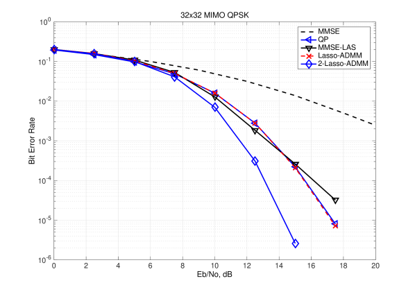
Figure 1: BER performance of QPSK $32\times 32$ MIMO

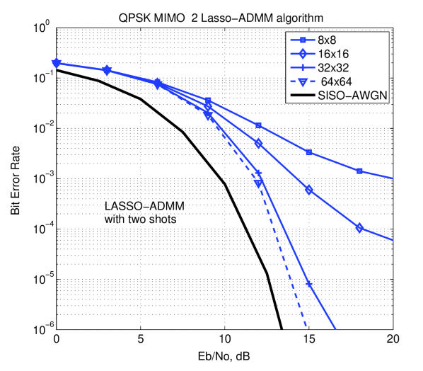
Figure 2: QPSK BER performance of 2 Lasso ADMM Algorithm for various $N_{t}\times N_{r}$ MIMO

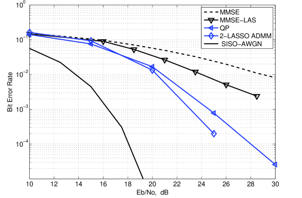
Figure 3: BER performance of 16QAM $32\times 32$ MIMO

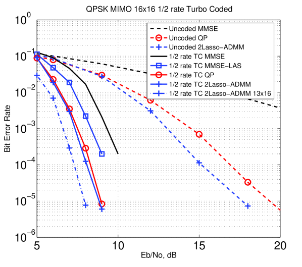
Figure 4: $1/2$ Turbo coded BER performance of QPSK

VI Conclusion and Future work

In this paper, a two-stage LASSO ADMM algorithm for large scale MIMO signal detection is investigated. Numerical results demonstrate the superiority of the proposed algorithm compared to the conventional methods for both coded and uncoded symbols at various QAM modulations. Investigating Multi-Stage LASSO-ADMM is an interesting future work.

References

• [1] F. Boccardi, R. W. Heath Jr, A. Lozano, T. L. Marzetta, and P. Popovski, “Five Disruptive Technology Directions for 5G,” IEEE Communications Magazine, vol. 52, no. 2, pp. 74–80, 2014.
• [2] Z. Zhang, X. Wang, K. Long, A. V. Vasilakos, and L. Hanzo, “Large-scale MIMO-based wireless backhaul in 5G networks,” IEEE Wireless Communications, vol. 22, no. 5, pp. 58–66, 2015.
• [3] K. Vishnu Vardhan, S. K. Mohammed, A. Chockalingam, and B. Sundar Rajan, “A low-complexity detector for large MIMO systems and multicarrier CDMA systems,” Selected Areas in Communications, IEEE Journal on, vol. 26, no. 3, pp. 473–485, 2008.
• [4] P. Li and R. D. Murch, “Multiple output selection-LAS algorithm in large MIMO systems,” Communications Letters, IEEE, vol. 14, no. 5, pp. 399–401, 2010.
• [5] B. S. Rajan, S. K. Mohammed, A. Chockalingam, and N. Srinidhi, “Low-complexity near-ML decoding of large non-orthogonal STBCs using reactive tabu search,” in Information Theory, 2009. ISIT 2009. IEEE International Symposium on.   IEEE, 2009, pp. 1993–1997.
• [6] N. Srinidhi, S. K. Mohammed, A. Chockalingam, and B. S. Rajan, “Near-ML signal detection in large-dimension linear vector channels using reactive tabu search,” arXiv preprint arXiv:0911.4640, 2009.
• [7] T. Datta, N. Srinidhi, A. Chockalingam, and B. S. Rajan, “Random-restart reactive tabu search algorithm for detection in large-MIMO systems,” Communications Letters, IEEE, vol. 14, no. 12, pp. 1107–1109, 2010.
• [8] A. Elghariani and M. Zoltowski, “Low complexity detection algorithms in large-scale MIMO systems,” IEEE Transactions on Wireless Communications, vol. 15, no. 3, pp. 1689–1702, 2016.
• [9] T. Takahashi, S. Ibi, T. Ohgane, and S. Sampei, “On normalized belief of Gaussian BP in correlated large MIMO channels,” in Information Theory and Its Applications (ISITA), 2016 International Symposium on.   IEEE, 2016, pp. 458–462.
• [10] R. Tibshirani, “Regression shrinkage and selection via the LASSO,” Journal of the Royal Statistical Society. Series B (Methodological), pp. 267–288, 1996.
• [11] E. Elhamifar and R. Vidal, “Sparse subspace clustering: Algorithm, theory, and applications,” IEEE transactions on pattern analysis and machine intelligence, vol. 35, no. 11, pp. 2765–2781, 2013.
• [12] J. Eckstein and D. P. Bertsekas, “On the Douglas-Rachford Splitting Method and the Proximal Point Algorithm for Maximal Monotone Operators,” Math. Program., vol. 55, no. 3, pp. 293–318, 1992.
• [13] J. Yang and Y. Zhang, “Alternating Direction Algorithms for $\ell\_1$-Problems in Compressive Sensing,” ArXiv e-prints, Dec. 2009.
• [14] S. Boyd, N. Parikh, E. Chu, B. Peleato, and J. Eckstein, “Distributed optimization and statistical learning via the alternating direction method of multipliers,” Found. Trends Mach. Learn., vol. 3, no. 1, pp. 1–122, Jan. 2011.
• [15] D. Boley, “Local linear convergence of the alternating direction method of multipliers on quadratic or linear programs,” SIAM Journal on Optimization, vol. 23, no. 4, pp. 2183–2207, 2013.
• [16] A. Elghariani and M. Zoltowski, “A quadratic programming-based detector for large-scale MIMO systems,” in WCNC, 2015 IEEE.   IEEE, 2015, pp. 387–392.