Accretion of clumpy cold gas onto massive black hole binaries: a possible fast route to binary coalescence

Abstract

In currently favoured hierarchical cosmologies, the formation of massive black hole binaries (MBHBs) following galaxy mergers is unavoidable. Still, due the complex physics governing the (hydro)dynamics of the post-merger dense environment of stars and gas in galactic nuclei, the final fate of those MBHBs is still unclear. In gas-rich environments, it is plausible that turbulence and gravitational instabilities feed gas to the nucleus in the form of a series of cold incoherent clumps, thus providing a way to exchange energy and angular momentum between the MBHB and its surroundings. Within this context, we present a suite of smoothed-particle-hydrodynamical models to study the evolution of a sequence of near-radial turbulent gas clouds as they infall towards equal-mass, circular MBHBs. We focus on the dynamical response of the binary orbit to different levels of anisotropy of the incoherent accretion events. Compared to a model extrapolated from a set of individual cloud-MBHB interactions, we find that accretion increases considerably and the binary evolution is faster. This occurs because the continuous infall of clouds drags inwards circumbinary gas left behind by previous accretion events, thus promoting a more effective exchange of angular momentum between the MBHB and the gas. These results suggest that sub-parsec MBHBs efficiently evolve towards coalescence during the interaction with a sequence of individual gas pockets.

1 Introduction

Massive black holes (MBHs) with masses between $\sim$$10^{6}-10^{10}M_{\odot}$ (Kelly & Shen 2013) have been observed to inhabit the nuclei of massive galaxies. And even though these objects are tiny with respect to their hosts, they are believed to play a fundamental, yet not fully understood, role in galaxy evolution. In fact, the observed tight correlations between the MBH masses and the properties of their galaxies (e.g. Magorrian et al. 1998; Ferrarese & Merritt 2000; Gebhardt et al. 2000) strongly suggest a coevolution scenario through feedback processes (Kormendy & Ho 2013, and references therein).

Furthermore, according to the currently favoured $\Lambda$CDM cosmology, galaxies assemble hierarchically through mergers following their parent dark matter haloes, building up from smaller structures (White & Rees 1978). A natural outcome of this process is the formation of massive black hole binaries (hereafter MBHBs). Following a merger of two galaxies, we expect both MBHs harboured in their nuclei to sink toward the centre of the merger remnant and eventually form a binary (Begelman et al. 1980). Therefore, understanding MBHB formation and dynamical evolution is a necessary piece for reconstructing the puzzle of the hierarchical growth of structures in the Universe. This is particularly interesting if we consider that MBHBs are powerful sources of gravitational waves (GWs), detectable by the future space-based laser interferometer space antenna (LISA, Consortium et al. 2013; Amaro-Seoane et al. 2017). For GWs to carry away enough energy, however, the two MBHs have to reach a separation of $a_{\rm GW}\sim 10^{-3}$ pc. This is extremely small compared to the $\approx 1$pc separation at which dynamical friction, initially driving the evolution of the two MBHs in the merger remnant, ceases to be efficient (Binney & Tremaine 2008).

The exact evolution and the final fate of the MBHs strongly depends on the content and distribution of both gas and stars in the galactic nucleus, and different processes can change dramatically the merging timescale, even resulting in values higher than the Hubble time. Although there is some indirect evidence that these binaries coalesce into a single object (e.g., the low scatter in the $M-\sigma$ relation, Jahnke & Macciò 2011), the processes involved are not completely understood.

For instance, due to its dissipative nature, gas can be very efficient in absorbing and transporting outwards the angular momentum of the pair, likely leading to a rapid evolution and eventual coalescence. From observations, as well as numerical simulations, it has been established that in gas-rich galaxy mergers there is a large inflow of gaseous material to the central kiloparsec of the galactic remnant, often resulting in a massive circumnuclear disc (Barnes & Hernquist 1992; Sanders & Mirabel 1996; Mayer et al. 2007). Driven by dynamical friction and global torques from this disc, the pair of MBHs decays very efficiently down to separations of the order of $\sim$ 1–0.1 pc, where it forms a gravitationally bound binary (Escala et al. 2004, 2005; Mayer et al. 2007; Fiacconi et al. 2013; Roškar et al. 2015; del Valle et al. 2015). At these sub-parsec scales, most theoretical and numerical studies have focused on the evolution of binaries surrounded by a gaseous circumbinary disc, often either co-rotating (see e.g. Ivanov et al. 1999; Armitage & Natarajan 2005; Cuadra et al. 2009; Haiman et al. 2009; Lodato et al. 2009; Nixon et al. 2011; Roedig et al. 2011, 2012; Kocsis et al. 2012; Amaro-Seoane et al. 2013; D’Orazio et al. 2013; Muñoz & Lai 2016; Miranda et al. 2017; Tang et al. 2017) or conuter-rotating (see e.g. Nixon & Lubow 2015; Roedig & Sesana 2014) with respect to the binary’s orbital motion. These discs are generally assumed to be well-defined, smooth, and relaxed, with no attempt to link their presence to the gaseous environment around the binary, nor to the fuelling mechanisms that bring gas to the nucleus. Furthermore, all these idealised scenarios are subject to the disc consumption problem, namely, if the disc dissolves through some process (e.g. star formation, AGN/supernovae feedback, Lupi et al. 2015), the evolution of the binary orbit stops. In fact, the evolution of MBHBs in gas-rich environments is intimately related to the unsolved problem of gas supply to the centre of galactic nuclei.

The fuelling of gaseous material onto galactic nuclei is currently a critical, yet uncertain piece in the galaxy formation puzzle. The wide range of physical scales involved makes the fuelling a very complex process – the gas needs to lose its angular momentum efficiently to be transported from galactic scales down to the nuclear region (Hopkins & Quataert 2011). A plausible mechanism that could break this angular momentum barrier is provided by chaotic feeding or ballistic accretion of cold streams when the gas is cold enough to form dense clouds or filaments (Hobbs et al. 2011).

Cold accretion onto black holes has long been predicted by both theory and simulations. The possible relevance of discrete and randomly oriented accretion events was first highlighted by King & Pringle (2006) (see also King & Pringle 2007; Nayakshin & King 2007; Nayakshin et al. 2012), which they referred to as “chaotic accretion” scenario. They argue that a series of gas pockets falling from uncorrelated directions could explain the rapid growth of MBHs across cosmic time, and can reproduce some of the observed properties (e.g. the $M_{\rm BH}-\sigma$ relation). One of the most extensive efforts to study the evolution of multiphase gaseous haloes and its impact on MBH accretion is the work of Gaspari and collaborators (Gaspari et al. 2012; Gaspari et al. 2013, 2015; Gaspari & Sa̧dowski 2017; Gaspari et al. 2017, 2018). By means of numerical simulations, they have shown that realistic turbulence, cooling, and heating affecting the hot halo, can dramatically change the accretion flow onto black holes, departing from the idealised picture of the Bondi prescription (Bondi 1952). Under certain physical conditions, cold clouds and filaments condense out of the hot phase due to thermal instabilities. Chaotic collisions then promote the funnelling of the cold phase towards the MBH, leading to episodic spikes in the accretion rate.

A likely example of this kind of discrete accretion events is the putative molecular cloud that resulted in the unusual distribution of stars orbiting our Galaxy’s MBH. Several numerical studies have shown that portions of a near-radial gas infall can be captured by a MBH to form one or more eccentric discs that eventually fragment to form stars (Bonnell & Rice 2008; Hobbs & Nayakshin 2009; Alig et al. 2011; Gaburov et al. 2012; Mapelli et al. 2012; Lucas et al. 2013; Mapelli & Trani 2016), roughly reproducing the observed stellar distribution (Paumard et al. 2006; Lu et al. 2009). An interesting feature of these observed stellar discs is that they appear to be misaligned with respect to the Galactic plane, indicating that the infalling gas had an angular momentum direction unrelated to that of the large scale structure of the Galaxy.

From an observational perspective, the development of multi-wavelength observations has started to unveil the multiphase structure of massive galaxies. These galaxies have been observed to harbour neutral and molecular gas down to $\sim$10 K (e.g. Combes et al. 2007). The Atacama Large Millimetre Array (ALMA) has opened the gate to high-resolution detection of molecular gas in early-type galaxies. For instance, there have been observations of giant molecular associations in the NGC5044 group within $r\lesssim$ 4 kpc, inferred to have chaotic dynamics (David et al. 2014). In massive galaxy clusters, ALMA has detected molecular hydrogen in the core of the Abell 1835 galaxy cluster (McNamara et al. 2014), which may be supported in a rotating, turbulent disc oriented nearly face-on. In the Abell 1664 cluster, the molecular gas shows asymmetric velocity structure, with two gas clumps flowing into the nucleus (Russell et al. 2014). More importantly, in a recent study, Tremblay et al. (2016) reported observations that reveal a cold, clumpy accretion flow towards a massive black hole fuel reservoir in the nucleus of the Abell 2597 galaxy cluster, a nearby giant elliptical galaxy surrounded by a dense halo of hot plasma. They infer that these cold molecular clouds are within the innermost hundred parsecs, moving inwards at about 300 kilometres per second, likely fuelling the black hole with gaseous material. The authors claim that this is the first time a distribution of molecular clouds has been unambiguously linked with MBH growth. Finally, Temi et al. (2018) have presented the detection of molecular clouds in three group centred elliptical galaxies (NGC 5846, NGC 4636, and NGC 5044) which are likely the result of condensation of the hot gas, and are consistent with a turbulent dynamics, as predicted by the cold chaotic accretion scenario (Gaspari et al. 2013).

Despite these several clues suggesting that stochastic condensation of cold gas and its accretion onto the central MBH is essential for active galactic nuclei, it has been barely explored as a possible source of gas for sub-parsec MBHBs. Notable exceptions are the studies of Dunhill et al. (2014), Goicovic et al. (2016, hereafter Paper I) and Goicovic et al. (2017, hereafter Paper II), where the Authors have numerically modelled the interaction of a single gaseous cloud with MBHBs for a variety of orbital configurations. In particular, Paper II extrapolated the results for these single cloud models to estimate the long-term evolution of a binary interacting with a sequence of near-radial infalling clouds, finding a very efficient shrinking of its orbit. However, the approach presented in Paper II is subject to a series of limitations, mainly, considering only the prompt evolution during the first impact of the clouds without the secular effects of the remaining gas. These effects can become very important after a series of accretion events due to the formation of circumbinary structures that can continue extracting angular momentum and increasing accretion onto the binary. With the goal of overcoming these limitations, we present a suite of hydrodynamical simulations of MBHBs interacting with a sequence of clouds, infalling incoherently onto the binary with different levels of anisotropy. These models now combine the ‘discrete’ evolution due to the prompt interaction of each individual cloud, with the secular torques exerted by the left-over gas.

This paper is organised as follows. We first describe our numerical model in Section 2, highlighting the main differences with respect to the studies presented in Paper I and Paper II. In Section 3 we show the dynamical evolution of the binary in response to the different levels of anisotropy of the accretion events, and by comparing with the single cloud extrapolations, we identify the effects of the non-accreted material. In Section 4 we study the same effects on a different suite of runs featuring an higher cloud supply rate. We finally summarise and discuss the implications of our results in Section 5. Unless stated otherwise, throughout this paper we use units such that $G=a_{0}=M_{0}=1$, where $G$ is the gravitational constant, and $a_{0}$, $M_{0}$ are the initial binary separation and mass, respectively.

2 The numerical model

We base our model of multiple clouds on the simulations presented in Paper I and Paper II. The new suite of simulations is fully described in the companion paper Maureira-Fredes et al. (2018). We model the interaction between the gas clouds and the MBHBs using the smoothed-particle-hydrodynamics (SPH) code gadget-3, an updated version of the public code gadget-2 (Springel 2005).

As described in Paper I, we modified the standard version of the code to include a deterministic accretion recipe, where the sink particles representing the MBHs accrete all bound SPH particles within a fixed radius ($r_{\rm sink}$) as implemented by Cuadra et al. (2006); we set this radius to $r_{\rm sink}=0.1a_{0}$. Additionally, we treat the thermodynamics of the gas using a barotropic equation of state (i.e. pressure is a function of density only) with two regimes; for densities lower than some critical value ($\rho_{c}$), the gas evolves isothermally, while for higher densities the gas is adiabatic. This prescription captures the expected temperature dependence with density of the gas without an explicit implementation of cooling, and has the effect of halting the collapse of the densest gas, avoiding excessively small time-steps that would stall the simulations. For the simulations presented in this paper we have chosen $\rho_{c}=10^{-2}M_{0}a_{0}^{-3}$, which is two orders of magnitude smaller than the value presented in Paper I and Paper II. This change is necessary to avoid stalling the simulations due to the formation of a large amount of clumps in some configurations. Since we are not following in detail the evolution of these clumps, stopping their collapse in a lower density should not affect greatly our results. This fact only becomes important when scaling our simulations to physical units – for the fiducial model presented in Paper I, where the binary has $M_{0}=10^{6}M_{\odot}$ and $a_{0}=0.2$ pc, the value of the critical density is now $\rho_{c}=10^{-16}$ g cm^-3, which is not necessarily an accurate representation of the collapse of molecular hydrogen (Masunaga & Inutsuka 2000).

To improve the orbit integration accuracy we have made changes with respect to the single cloud models presented in Paper II. First, we have modified the code to remove the sink particles from the gravity tree approximation, and their forces are instead summed directly. In simple words, each sink particle sees all other particles individually. Additionally, the orbit of the black holes is integrated using a fixed time-step, set equal to $\Delta t_{\rm sink}=0.02P_{0}$.

A more critical modification with respect to the previous simulations is the frequency at which the code makes the domain decomposition and full tree reconstruction. The single cloud models of Paper II had sufficient resolution to study the transient evolution of the binary during the first impact of the gas. Conversely, the typically much smaller secular torques exerted by the remaining gas were not resolved. The main source of this numerical noise is the aforementioned frequency, more specifically, when the tree reconstruction is not done at the same time with the black hole accretion, the sudden disappearance of particles during an update creates spurious jumps in the total angular momentum, which are generally larger than the small torques that we are trying to resolve with these models. In order to improve the conservation of angular momentum, we modified gadget to enforce the domain decomposition and full tree reconstruction every time the sink particles are active. This implementation is complementary to the standard criterion based on the amount of active particles (Springel 2005). While this greatly increases the computational cost (typically by a factor of $\sim$10), the numerical fluctuations in the total angular momentum are vastly reduced, allowing a robust study of its dynamical evolution during all phases of the interaction (see below).

Considering the aforementioned modifications, and to make these simulations feasible, we have decreased the resolution elements of the individual clouds with respect to the single cloud models. We model the gas clouds using $5\times 10^{4}$, $2\times 10^{5}$, $5\times 10^{5}$ and $10^{6}$ particles (in contrast with the $4\times 10^{6}$ used before) to evaluate the convergence of our results with resolution. To identify these different resolutions throughout this paper we use 50k, 200k, 500k and 1m, respectively.

2.1 External potential

In the single cloud simulations presented in Paper I and Paper II, the system was treated in isolation, i.e. with no external forces acting upon it. In reality, such a binary would be placed deep in the potential well of a galaxy, where stars and dark matter exert their gravitational influence. To mimic the presence of the galactic spheroid we include an external potential with a Hernquist profile (Hernquist 1990) which can be written as

$$\rho(r)=\frac{M_{*}}{2\pi}\frac{a_{*}}{r}\frac{1}{(r+a_{*})^{3}},$$ (1)

and an enclosed mass given by

$$m(r)=M_{*}\frac{r^{2}}{(r+a_{*})^{2}},$$ (2)

where $M_{*}$ and $a_{*}$ are scaling constants that represent the total mass of the spheroid and the size of core, respectively. Based on a typical $M_{\rm BH}-M_{\rm bulge}$ relation (Magorrian et al. 1998) and a radius-to-stellar-mass relation (Dabringhausen et al. 2008), we choose $M_{\rm H}=4.78\times 10^{2}M_{0}$ and $r_{\rm H}=3.24\times 10^{2}a_{0}$, thus implying

$$m(a_{0})\approx 5\times 10^{-3}M_{0}.$$ (3)

As a consequence, this external force represents only a small perturbation to the dynamics of the interaction that is still dominated by the binary’s gravitational potential. Moreover, because this external potential is spherically symmetric, orbits experience precession only, where energy and angular momentum are conserved. In principle, this precession could enhance stream collisions, prompting more gas onto the binary, although the timescales are too long with respect to the frequency of cloud infall, which is the dominant effect in our models. Based on this, we do not expect the oscillations induced by this potential to have a secular effect in the overall evolution of the system during the stages modelled. In practice, this potential maintains the binary close to the centre of the reference frame by applying a restoring force when it drifts away due to the interaction with the incoming material. It is important to mention that the gas also feels this external force.

For the single cloud simulations this potential was not needed, as drifts produced by the interaction with the cloud or by numerical inaccuracies did not affect the prompt phase studied. For the simulations presented here, however, this restoring force guarantees that the orbit of each cloud remains close to the originally calculated values, as the pericentre distance for each cloud was computed assuming the binary’s centre of mass static at the origin of the Cartesian coordinates.

2.2 Initial conditions

The binary consists of two sink particles, initially having equal masses and a circular orbit in the $x-y$ plane. On the other hand, all the clouds are initially spherical with uniform density, a turbulent velocity field, and a total mass 100 times smaller than the binary (i.e. $M_{c}=0.01M_{0}$). And similar to the single cloud models, the turbulent velocity field is drawn from a random distribution with power spectrum $P_{v}(k)\propto k^{-4}$. It is worth mentioning that the random seed is exactly the same for all clouds. With these choices all clouds are identical except for their initial orbit, which simplifies the comparison between the different distributions.

Figure 1: Angular momentum orientations of the initial orbit for 20 randomly selected clouds from different $F$ distributions, as indicated at the top of each projection. The binary’s angular momentum initially points to the north pole $(\theta=90^{\circ})$ on these projections. Note that $F=0.0$ and $F=1.0$ cloud orbits are generated by mirroring the inclination angle $\theta$ from $F=0.5$ with respect to the binary’s orbital plane (red solid line) to swap between one hemisphere to the other. Labelled numbers on each circle indicate the order in which we introduce the clouds.

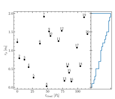
Figure 2: Distribution of pericentre distances as a function of the time at which each cloud is included to the simulation. This distribution is used for the 3 levels of anisotropy $F$ shown in Fig. 1. The labelled numbers indicate the order of the clouds. The right plot shows the cumulative distribution of pericentre distances.

The initial setup of these simulations is motivated by the Monte Carlo models presented in Paper II, and is described in full detail in Maureira-Fredes et al. (2018). We use the $F$-distributions to model the different levels of anisotropy of the cloud distribution, where the number $F$ represents the fraction of counter-rotating events with respect to the binary (southern hemisphere of the projections shown in Fig. 1). On the other hand, we use a flat distribution of pericentre distances. This choice stems from the dynamics seen in simulations of cold clump dynamics Gaspari et al. (2013). Gaseous clumps condensing out of the interstellar medium suffer many chaotic collisions that redistribute their orbital angular momenta. At small orbital angular momenta values – i.e. for clouds falling onto the galactic center – a uniform reshuffling results in a $p(b)\propto b\differential b$ impact parameter distribution which, in turn, produces a flat distribution of pericentre distances due to gravitational focusing of the MBHB.

We generate a total of 20 clouds with orientations shown in Fig. 1 and periapsis shown in Fig. 2. Note that the same pericentre distances are used for the 3 different levels of anisotropy $F$. We set the maximum value of the pericentre distance to $r_{\rm p,max}=2a_{0}$, to ensure a transient evolution with the first impact independent of the cloud’s relative inclination (see Paper II). Although the exact choice of maximum value is somewhat arbitrary, Dunhill et al. (2014) demonstrated that the effect on the binary semimajor axis produced by clouds with larger impact parameters is negligible.

Finally, the time difference between events exhibited on Fig. 2 was determined from a Gamma distribution with shape 2 and a scale parameter of $\theta=2.5P_{0}$. The average time between successive injections is $\Delta t\approx 6P_{0}$. For a binary with $M_{0}=10^{6}M_{\odot}$ and $a_{0}=0.2$ pc, this rate of clouds corresponds to a mass inflow of $\approx 0.2M_{\odot}$ yr^-1 entering the inner parsec. Note that the arrival rate of clouds is a free parameter in our model, and can have important consequences on the evolution of the binary (see comparison in §4, and also Maureira-Fredes et al. 2018). It is therefore important to fix it to a physically motivated value. Our choice ensures that the resulting mass inflow rate is in broad agreement with inflow rates onto single MBHs found by numerical studies about the formation and infall of cold clumps (e.g. Hobbs et al. 2011; Gaspari et al. 2013, 2015; Fiacconi et al. 2018). These models show, however, that the gaseous inflow critically depends on the different physical mechanisms acting on the interstellar medium, hence future observational campaigns are needed to better constrain the typical rate of these discrete accretion events on galactic nuclei.

In order to make a robust comparison of the dynamical impact of each distribution it is necessary to reduce some of the stochasticity produced by the low number of events. With that goal in mind, the different angular momentum distributions were not sampled independently from each other. Only the angles from the isotropic distribution ($F=0.5$) are randomly drawn. We then generate the co-rotating distribution ($F=0.0$) by reflecting symmetrically the negative inclination angles ($\theta<0^{\circ}$) with respect to the binary’s orbital plane onto the northern hemisphere. The same is done to get the counter-rotating distribution ($F=1.0$), but mirroring the angles $\theta>0^{\circ}$ onto the southern hemisphere. The azimuthal angles are kept unchanged. This means that the only difference between distributions is the inclination angle $\theta$ of the cloud’s orbits.

Because we are modelling 3 levels of anisotropy for the incoming clouds and we are performing runs at four different resolutions, we are presenting a total of 12 simulations, corresponding to RunB in Maureira-Fredes et al. (2018). We concentrate our analysis on this set of runs because we were able to evolve all the three 50k simulations up to the 20th cloud, thus providing a consistent dataset for the analysis. RunA of Maureira-Fredes et al. (2018) yields similar results, which we summarise in §4.

All the simulations described in this paper are run in different ‘segments’. Initially one cloud is placed with the corresponding initial position and velocity vectors. This system is evolved until the time set for the following cloud to enter has been reached; at this point we stop the simulation. The new cloud is added to the final snapshot to generate the initial conditions for the following section.

3 Dynamical evolution of the binary

3.1 Angular momentum

Figure 3: Angular momentum evolution for the lower resolution runs (50k). The upper panels of each plot show the evolution of the angular momentum magnitude of the entire system (red solid lines) and the binary (dashed blue lines). The dotted light blue lines represent the contribution of the semimajor axis evolution to the binary’s angular momentum, while the dotted-dashed orange lines are the contribution of the total mass change, as shown in equation (5). The lower panels display the relative change between consecutive snapshots of the same lines. The vertical shaded areas indicate the arrival time of the clouds. The extreme “jumps” seen in the red lines are caused by new clouds entering the system, thus providing additional angular momentum. The top row of plots show the evolution during the entire simulations, while the bottom row is a zoom-in on the first $\approx 12$ orbits, which shows in detail the interaction with 2 clouds.

The first step is to establish whether the simulations have the accuracy to measure the effects of the interaction between the binary and the sequence of clouds. With this goal in mind, we measure the conservation of angular momentum in the different models, as shown in Fig. 3. This corresponds to the evolution in the lower resolution simulation, but because the binary evolution is almost independent from the number of particles (see below), these examples illustrate the evolution of the higher resolution models as well.

Consistent with the single cloud models, the largest effect in the binary angular momentum occurs during the interaction with the first incoming material, depicted as vertical shaded areas. The fluctuations following the first encounter with each cloud rapidly decrease. It is important to clarify that the rather extreme jumps observed in the total angular momentum are not numerically driven, but produced by the addition of new clouds into the system. From the lower panels of Fig. 3 it is clear that this does not translate into spurious jumps in the binary evolution, as there are no such noticeable changes in its angular momentum. Moreover, simulation’s segments delimited by the addition of clouds are extremely flat, i.e. the numerical fluctuations in the total momentum are way below the observed binary evolution and consequently they can hardly be seen at this scale. This implies that the new models, thanks to the frequent tree updates, have the numerical accuracy to resolve the binary evolution beyond the prompt phase, as opposed to the old single cloud simulations.

From the top panels of Fig. 3 it is possible to observe that the evolution of the binary is somewhat following the injection of momentum in the form of clouds. In other words, the binary increases its angular momentum in the $F=0.0$ model, where as in the $F=1.0$ model the opposite occurs and it decreases. For the isotropic case ($F=0.5$) the angular momentum increases and decreases depending on whether the new cloud is co-rotating or counter-rotating, respectively. Although we expect a monotonically increasing angular momentum in the $F=0.0$ simulation, the small drops caused by the inclusion of clouds 11, 12, 16 and 19 occur because the binary inclination slightly changes during the simulations. Said clouds, being so close to the initial binary’s orbital plane (see Fig. 1, upper panel), are now located in the southern hemisphere of the binary at the time of inclusion.

The behaviour of the binary’s angular momentum is in agreement with our previous results where the main effect of the infalling material is to exchange its angular momentum through capture and accretion (Paper II). It is important to bear in mind that an increase in the binary angular momentum does not necessarily imply an expansion of the semimajor axis; this only means that the contribution of the total accreted mass, which is always positive, is much larger to that of the likely negative semimajor axis. This can be understood similarly to what is shown in Paper II, where we write the binary angular momentum in terms of its parameters as follows:

$$L_{\rm bin}=\frac{q}{(1+q)^{2}}M^{3/2}\sqrt{Ga(1-e^{2})},$$ (4)

where $G$ is the gravitational constant. By differentiating we find that at first order this expression implies

$$\frac{\Delta{L_{\rm bin}}}{L_{\rm bin}}=\frac{1-q}{q(1+q)}\Delta{q}+\frac{3}{2}\frac{\Delta{M}}{M}+\frac{1}{2}\frac{\Delta{a}}{a}-\frac{e}{1-e^{2}}\Delta{e}.$$ (5)

Similar to the single cloud models, during all of our simulations the binary remains roughly equal-mass and circular. We can therefore calculate approximately the total change in angular momentum based on the change in $a$ and $M$ only,

$$\frac{\Delta{L_{\rm bin}}}{L_{\rm bin}}\approx\frac{3}{2}\frac{\Delta{M}}{M}+\frac{1}{2}\frac{\Delta{a}}{a}.$$ (6)

The contributions of both semimajor axis and mass terms are displayed in the upper panels of Fig. 3. From there it is clear that the addition of these two terms is sufficient to reproduce the binary’s angular momentum evolution, justifying our approximation of ignoring the mass ratio and eccentricity contributions. It is also evident that the $\Delta a$ contribution to the MBHB angular momentum change is always negative, indicating that the binary shrinks also when $\Delta L_{\rm bin}>0$.

3.2 Orbital elements

Figure 4: Evolution of the binary semimajor axis (top panels), eccentricity (upper-middle panels), total accreted mass (lower-middle panels), and accretion rate (bottom panels) for all the simulations. The corresponding distribution is indicated at the top of each plot. The different lines in each panel represent the cloud resolutions, as indicated in the legend. The vertical shaded areas indicate the arrival times of the clouds. Note that the non-solid lines are arbitrarily shifted either upwards or downwards with respect to the solid line (50k resolution) in the semimajor axis, accreted mass and accretion rate panels for clarity. The virtually identical evolution during these stages indicates convergence with the number of particles per cloud.

On the basis of the adequate angular momentum conservation, it is possible to study the evolution of the binary orbital elements during the entirety of the simulations. To properly include the influence of the external potential on the binary, we compute its orbital elements ($a$ and $e$) using the periapsis and apoapsis, instead of the relative energy and angular momentum of the two MBHs. Figure 4 displays the time evolution of the semimajor axis, eccentricity, total mass and accretion rate comparing the different resolutions modelled. Because the different resolutions tend to lie on top of each other, we arbitrarily shifted the non-solid lines with respect to the solid line (50k resolution) for the semimajor axis, accreted mass and accretion rate, which is indicated by black arrows. The virtually identical orbital evolution during the modelled stages indicates convergence with the number of particles per cloud. This is because the dynamical evolution of the system is dominated by capture and gravitational slingshot, which are properly resolved even with a low number of particles. The largest differences are present in the eccentricity evolution. This is due to the typically low values ($e\lesssim 0.02$) of this quantity that makes it much more sensitive to noise. Although the sources of this noise are difficult to identify, the dependence with particle number suggests that the details of the accretion are likely playing an important role. Due to the symmetries of our configuration, the binary mass ratio remains robustly around unity throughout the modelled stages, but with some stochastic small deviations on top. Considering equation (5), for a given change of $L_{\rm bin}$, $M$ and $a$, changes in $\mu$ and $e$ are highly entangled. For this reason we restrict the analysis to the semimajor axis and mass evolution. In any case, all our binaries remain essentially circular over the modelled timescales (although they consistently show a mild tendency to increase eccentricity), and the small discrepancies in eccentricity do not affect the overall evolution of the system.

Similar to the results shown in Paper I, the accretion rate onto the binary presents a very clear periodicity at half the binary’s orbital period (or twice the binary frequency). This is mainly a dynamical effect, associated with streams of gas that feed each black hole alternately when they intersect. We do not identify any other persistent trends in the accretion rates. Variability related to the binary orbital period is the type of behaviour that we expect will help to identify and characterise these systems, as it could appear in AGN light curves and be detected by future time-domain surveys, and it has been extensively studied with numerical simulations of quasi-steady circumbinary discs (e.g. MacFadyen & Milosavljević 2008; Cuadra et al. 2009; Roedig et al. 2011; Shi et al. 2012; D’Orazio et al. 2013; Dunhill et al. 2015; Farris et al. 2015a; D’Orazio et al. 2015; Shi & Krolik 2015; Muñoz & Lai 2016; Tang et al. 2017, 2018). Note that for our fiducial scaling the binary period is several thousands of years, certainly too long to be observed (see Table 2 in Paper I, for different scalings of these systems). However, we expect that the behaviour we find is qualitatively representative of those more rapidly varying systems, especially if there is a steady supply of clouds reaching the galactic nucleus.

Table 1: Total change of the binary semimajor axis ($\Delta a$) and mass ($\Delta M$) for the different models at the final time ($T_{\rm fin}$) of the simulations. The model name is composed of the $F$ distribution followed by the resolution of the individual clouds. $T_{\rm fin}$ is the final time reached by each simulation. The values with subscript ‘10th’ correspond to the total change after the interaction with the 10th cloud, which is measured at $t=65P_{0}$. This point was not reached by the higher resolution runs of $F=1.0$ distribution.

Model	$T_{\rm fin}$	$\Delta a$	$\Delta M$	$\Delta a_{\rm 10th}$	$\Delta M_{\rm 10th}$
	($P_{0}$)	($a_{0}$)	($M_{0}$)	($a_{0}$)	($M_{0}$)
F0.0_50k	145.4	-0.160	0.158	-0.079	0.056
F0.0_200k	95.7	-0.157	0.110	-0.075	0.057
F0.0_500k	79.7	-0.094	0.062	-0.079	0.057
F0.0_1m	68.2	-0.083	0.057	-0.078	0.056
F0.5_50k	126.0	-0.325	0.165	-0.218	0.064
F0.5_200k	86.7	-0.266	0.094	-0.222	0.065
F0.5_500k	69.7	-0.233	0.069	-0.221	0.064
F0.5_1m	67.1	-0.227	0.070	-0.221	0.067
F1.0_50k	124.0	-0.714	0.164	-0.405	0.070
F1.0_200k	81.5	-0.555	0.099	-0.428	0.073
F1.0_500k	68.2	-0.398	0.070	-0.371	0.065
F1.0_1m	42.7	-0.207	0.033	-	-

In Table 1 we compile the total change in both binary semimajor axis and total mass for all the simulations. The first 3 columns show the values measured at the end of each run ($T_{\rm fin}$), As expected, increasing the number of particles per cloud makes the simulations more computationally expensive, forcing us to stop them earlier in the evolution of the system. Additionally, the $F=1.0$ models are more expensive than the others because counter-rotating clouds tend to form more clumps. In order to facilitate the comparison between different resolutions, the values with subscript ‘10th’ correspond to the total change after the interaction with the 10th cloud, measured at $t=65P_{0}$, point that was reached by most of our simulations. Notice that, for a given $F$ distribution, the discrepancies on the binary parameters at this point are very small, being usually less than 5% with respect to the actual changes measured along the simulation.

Based on the results showed in Fig. 4 and the convergence of the simulation with resolution, most of the analysis in this paper is based on the 50k runs because more clouds have interacted with the binary. We expect the conclusions we will reach will apply for the higher resolution simulations.

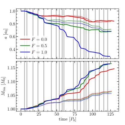
Figure 5: Time evolution of the binary semimajor axis (top panel) and mass (bottom panel) in the 50k runs for the different cloud distributions, as indicated in the legend. The solid lines depict the evolution measured directly from the simulations, while the dashed lines correspond to predictions based on the results from the single cloud model presented in Paper II. Similar to previous figures, the shaded vertical areas illustrate the start of the interaction of the binary with a new cloud.

To highlight the differences between distributions, in the upper panel of Fig. 5 we display the semimajor axis evolution for the three levels of anisotropy, while the lower panel shows the mass evolution. The solid lines on this figure represent the evolution measured from the simulations. As expected, the binary shrinks more efficiently when we increase the fraction of retrograde events. For instance, after the infall of 10 clouds the orbit shrinks by $\Delta a/a\approx 40\%$ in the $F=1.0$ simulation, by $\Delta a/a\approx 20\%$ in the $F=0.5$ model and by a mere $\Delta a/a\approx 8\%$ for $F=0.0$ (see Table 1). This can be understood in terms of the exchange of angular momentum with the captured material, as studied in detail in Paper II. Because retrograde clouds bring negative momentum to the binary, any captured and accreted material would immediately subtract angular momentum, while clouds with angular momentum closely aligned to $L_{\rm bin}$ tend to actually expand the MBHB orbit (see Fig. 6 in Paper II). In contrast with the semimajor axis, the total mass evolution remains very similar for the three levels of anisotropy, as the capture of material does not depend strongly on the orbit of the incoming gas. However, because the gas exchanges its angular momentum with the accreting black holes, the net effect in the binary orbit does depend on the different relative inclinations.

In the Monte Carlo models presented in Paper II, we have extrapolated the results from the single cloud simulations to evolve a binary embedded in a clumpy environment where individual gas pockets infall with different levels of anisotropy. One of the critical assumptions made in this approach was ignoring the effects of the left-over material after the first stages of the interaction. To investigate this effect we compute the binary evolution following the same procedure explained in Paper II, i.e. estimating the total change in mass and semimajor axis based on the cloud’s initial orientation and pericentre distance, using the values extrapolated from the single cloud models. In this procedure we are ignoring any secular effects from the non-accreted gas (as well as cloud-cloud interactions), by considering only the evolution measured during the prompt accretion phase. The results obtained are shown with dashed lines in Fig. 5.

During the interaction with the first few clouds the single cloud predictions agree well with the measured binary evolution, but after few events this simple model consistently underestimates both semimajor axis and mass evolution. This departure allows us to directly measure the effects of the surrounding material, previously unresolved with the Monte Carlo models in Paper II. In the following subsections, we analyse two effects: i) enhancement in accretion due to the interaction of the new incoming material with the gas already in orbit, and ii) gravitational torques from long-lived circumbinary gas structures.

It is important to stress that we always expect a departure between the combined effect of multiple clouds with respect to the extrapolation from the single cloud models, independent of the infall rate, since the latter lacks the aforementioned secular effects. For the relatively high frequency of clouds presented in this paper, this deviation is already clear, and is dominated by enhanced accretion as we show below. On the other hand, for a very low infall frequency, the surviving material would be allowed to settle into a circumbinary disc that exerts some small but persistent gravitational influence on the binary, continuing to extract its angular momentum (e.g. Cuadra et al. 2009).

3.2.1 Enhanced Accretion

Figure 6: Time evolution of the accreted mass contributed by each cloud in the different runs. Note that the mass is presented in unit of $10^{-2}M_{0}$, which corresponds to the initial mass of each cloud, thus the $y$-axis can be interpreted as the fraction of the cloud that has been accreted by the binary. Here we observe that some of the incoming clouds produce spikes also in the previous clouds.

One striking difference with respect to the single cloud extrapolations is the total accreted mass by the binary. From the lower panel of Fig. 5 we notice that the single cloud model underestimates the final mass by a factor of $\sim$3. This occurs because there is an accumulation of material around the binary, and the new incoming clouds are able to drag some of it, increasing accretion and consequently the effect on the binary semimajor axis. Note that the deviation of the measured evolution from the predicted one is episodic rather then continuous.

To corroborate this point, we present the contribution from each individual cloud to the mass accreted by the binary in Fig. 6. Here it is possible to observe that some of the incoming clouds produce an accretion spike also in some of the previous clouds. For example, one of the most noticeable cases is the arrival of cloud 8, which brings to the binary a significant fraction of clouds 1, 3 and 6. Recall from Fig. 2 that the 8th cloud has the smallest pericentre distance, very close to zero. This event produces the largest accretion in all distributions. This extra-accretion triggered by interactions with leftover gas from previously infalling clouds is obviously not captured by the simple model derived from the single cloud simulations. Additionally, since the capture of retrograde material is more efficient in shrinking the binary orbit, this enhancement in accretion translates into larger deviations when increasing the fraction of counter-rotating clouds, although it is hard to see this trend due to the scatter introduced by the specific cloud realisations. For instance, in the $F=0.5$ case shown in Fig. 5 the binary evolution is only slightly accelerated with respect to the single cloud extrapolation, while in the additional set of simulations shown in Fig. 15, the difference is much larger. It is important to notice that this is a ‘one way’ effect: interactions with multiple clouds consistently tend to accelerate the binary evolution.

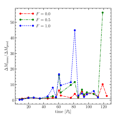
Figure 7: Time evolution of the ratio between the total accreted mass measured from the simulations and the value predicted from the single cloud models. The horizontal dotted line indicates $y=1$. This plot shows that the departure from the predicted accreted mass is stronger when there are circumbinary structures present.

Finally, in order to quantify the total increase of the accretion due to the accumulation of gas around the binary, we compute the evolution of the ratio between the total accreted mass measured from the simulation and the value predicted using the single cloud models, which is shown in Fig. 7. As previously observed, the prediction and the actual evolution agree reasonably well during the first few clouds, and this ratio oscillates around 1. After the build up of material around the binary, however, there are large bursts of accretion, reaching values up to $\gtrsim 50$ times the predicted level. This picture becomes stronger if we consider that around $t=60P_{0}$, following the infall of the 10th cloud, there are circumbinary discs formed in all the 3 distributions (see next subsection). These discs are disrupted at least partially by the new incoming clouds, promoting accretion onto the binary.

In a companion paper (Maureira-Fredes et al. 2018), we are using the same suite of simulations to study in detail the formation and evolution of gaseous structures arising from these sequences of infalling clouds onto a binary. In particular, we focus our analysis in the dependency with the level of anisotropy of the incoming clouds (expressed in terms of the $F$-distributions) and the time difference between events. There we show that is typically very difficult to build a substantial circumbinary disc in this scenario of incoherent accretion events, especially with shorter times in between clouds, because the incoming gas constantly perturbs the arising structure. Nevertheless, we do observe the formation of transient circumbinary structures that exert some gravitational influence on the binary’s orbit, as we discuss below.

3.2.2 Circumbinary disc formation and secular evolution

As thoroughly discussed in Paper II, another effect expected from the left-over gas is the formation of circumbinary structures. This represents one of the most important limitations of the models based on the single cloud simulations. For instance, in the extreme case where every cloud comes exactly coplanar and corotating with the binary (sometimes referred to as the ‘prolonged accretion’ scenario), the extrapolation from the single cloud models predicts that the semimajor axis would only increase. In reality, however, following several of such accretion events a massive circumbinary disc is expected to form. This structure can continue extracting and transporting the binary angular momentum, evolving the binary towards coalescence.

Figure 8: Column density maps of an intermediate output from models $F=0.0$ (left), $F=0.5$ (centre) and $F=1.0$ (right). For reference, the binary lies on the $x$-$y$, rotating counter-clockwise. The top and bottom panels show a face-on and edge-on view of the circumbinary structure formed after the interaction with 10 gaseous clouds. For the $F=0.0$ and $F=0.5$ models, the disc is prograde with respect to the binary orbit, while for the $F=1.0$ model the structure is retrograde.

Following the arrival of the 10th cloud, there is enough time before the next event for the gas to settle in a well-defined coplanar circumbinary structure in the 3 distributions. This can be clearly seen on the density maps shown in Fig. 8. For the $F=0.0$ and $F=0.5$ models, we observe the formation of a corotating circumbinary disc, while for the $F=1.0$ model the structure is a retrograde and much narrower, ring-like circumbinary disc.

Figure 9: Density maps averaged over 5 binary orbits for the $F=0.0$ (left), $F=0.5$ (centre) and $F=1.0$ (right) models. These maps were computed in a reference frame corotating with the binary. Note that the large amount of clumps seen in these panels are due to few clumps caught at different orbital phases when creating the maps by superimposing the snapshots. For the $F=0.0$ and $F=0.5$ distributions, there are gaseous streams leaking through a cavity sustained by the gravitational influence of the binary. In contrast, for the $F=1.0$ distribution the gas is able to orbit much closer, directly impacting the black holes.

To study any persistent structures of these developing discs we present the column density maps averaged over five orbits (100 snapshots) in Fig. 9. These maps were computed in a reference frame corotating with the binary, with the black holes aligned on the $x$-axis. It is clear that the gaseous structures are better defined in the $F=0.0$ simulation, where the binary has opened a clear cavity and each MBH is surrounded by prominent mini-discs. In contrast, the less coherent infall of material in the $F=0.5$ simulation delays the emergence of these features. Nevertheless, in both cases there is a dense, roughly circular ring of gas located at $r\approx 2a$. In this region the material piles up due to resonances with the gravitational potential of the binary (Artymowicz & Lubow 1994). Although the gravitational forces keep most of the gas confined at this radius, some material leaks thorough the cavity in the form of narrow streams that reach the black holes, a result that has been extensively reported in the literature (e.g. Artymowicz & Lubow 1996; MacFadyen & Milosavljević 2008; Cuadra et al. 2009; Roedig et al. 2012; D’Orazio et al. 2013; Farris et al. 2015b; Dunhill et al. 2015; Tang et al. 2017). Such inflowing gas can exert a net negative torque inside the cavity region, shrinking the binary more effectively than the resonant torques.

In contrast, we observe the formation of a counter-rotating circumbinary ring in the $F=1.0$ run. Because of the absence of gravitational resonances for counter-rotating material, the gas is able to orbit much closer to the binary, directly impacting onto the black holes. As a consequence, the morphology of the gas is quite different, as there are no mini-discs, nor gas in the form of streams. These features are extensively discussed in Maureira-Fredes et al. (2018).

Figure 10: Torque radial profiles averaged over the last five binary orbits. In each panel, the green dashed line represents the differential torque, while the red solid line is the total integrated torque. This latter is integrated starting from the corotation radius (vertical dotted line) inwards and outwards. The quantities are presented in code units, namely, $[GM_{0}^{2}a_{0}^{-2}]$ for the differential torque and $[GM_{0}^{2}a_{0}^{-1}]$ for the integrated profile.

To establish the role of the discs in the binary evolution we compute the gravitational torques exerted by the gas. The total gravitational torque is given by directly summing the individual particle torques onto each MBH as follows

$$\mathbf{T}_{g}=\sum_{i=1}^{N}\sum_{j=1}^{2}\mathbf{r}_{j}\crossproduct\frac{GM_{j}m_{i}}{\absolutevalue{\mathbf{r}_{i}-\mathbf{r}_{j}}^{3}}(\mathbf{r}_{i}-\mathbf{r}_{j}),$$ (7)

where the index $i$ runs over all the gas particles in the simulation, and $j=1,2$ indicates the two black holes. Using this expression, we compute the torque radial profiles shown in Fig. 10, averaged over 5 orbits of the simulation. As the binary’s inclination slightly evolves in our simulations, we compute these torques in a reference frame in which the binary angular momentum is exactly aligned with the $z$ axis. With this choice, we can directly link the $z$ component of the torque with the binary orbital evolution (eq. 5). Because the torques are null at the corotation radius, the integration of the differential profile is done from that point outwards and inwards.

From the profiles shown in Fig. 10 it is clear that the net effect of the circumbinary material is to produce a negative torque, hence to extract some angular momentum from the binary. For the co-rotating discs, the largest peak is located between $a$ and $2a$, i.e. inside the cavity wall. This peak basically determines the total strength of the torque, which is responsible for the shrinking observed in the binary orbit. Beyond the cavity region the torques oscillate between positive and negative, cancelling each other out, and consequently making the contribution of the disc negligible. For the counter-rotating disc, conversely, the gravitational torques come from the material inside the corotation radius, very close to the MBHs, and the outward torques are essentially absent because of the lack of Lindblad resonances.

Figure 11: Averaged surface density torque exerted by the gas onto the binary for the $F=0.0$ (left), $F=0.5$ (centre) and $F=1.0$ (right) models. Similar to the previous figures, these maps were averaged over five orbits. Note that the torque values for the minidiscs are off the scale in both $F=0.0$ and $F=0.5$ models. For the prograde discs this shows that the negative torques come from the gaseous streams reaching the binary. Conversely, in the counter-rotating disc these torques are located much closer to the binary.

To identify the location of the negative torques, we show the averaged surface density torque of the discs in Fig. 11. For the co-rotating circumbinary discs, and similar to the gas distribution shown in Fig. 9, the location of the torques are clearer in the $F=0.0$ model, where the cavity has been almost completely depleted of gas. Nonetheless, in both $F=0.0$ and $F=0.5$ cases the gaseous streams inside the cavity provide a strong source of negative torque. This confirms that the negative peak observed in the profiles of Fig. 10 comes from the material leaking through the cavity wall. Rather than being entirely captured by the binary, a fraction of this gas is flung back to the disc, via gravitational slingshot, carrying away angular momentum from the binary. This physical effect has been identified and extensively studied in the literature, mainly by means of numerical simulations (e.g. Roedig et al. 2012; D’Orazio et al. 2013; Farris et al. 2015b; Dunhill et al. 2015; Tang et al. 2017).

On the other hand, gravitational torques in the counter-rotating disc are located much closer to the binary, with no features resembling the gaseous streams as in the previous cases. This material extracts some of the binary’s angular momentum, but because it is not able to transport it outwards, this material is eventually accreted by the MBHs. As this gas is counter-rotating with respect to the binary, its capture and subsequent accretion subtracts angular momentum much more efficiently than in the co-rotating case (Nixon et al. 2011).

The profiles shown in Fig. 10 can be directly compared with results from previous studies of “standard” circumbinary discs. In particular, the simulations of a massive self-gravitating circumbinary disc by Roedig & Sesana (2014) find very similar torque profiles (cf. their Fig. 4), the main distinction being the strength of the peaks – the torques found in our simulations are noticeably larger. For instance, for prograde discs, Roedig et al. show a total outwards torque of $\sim 2\times 10^{-5}$ $[GM_{0}^{2}a_{0}^{-1}]$, while in our simulations we find it to be $\sim 4\times 10^{-5}$ $[GM_{0}^{2}a_{0}^{-1}]$, hence a factor of $\sim 2$ larger. In the retrograde case, Roedig et al. find a total integrated torque of $\sim 10^{-5}$ $[GM_{0}^{2}a_{0}^{-1}]$, while we find $\sim 5\times 10^{-5}$ $[GM_{0}^{2}a_{0}^{-1}]$, a factor of $\sim 5$ larger. Even though these values might not seem much higher, note that we are comparing very massive circumbinary discs with 20% the binary mass to the much lighter discs formed in our simulations, that reach at most a few percent of the MBHB mass (Maureira-Fredes et al. 2018).

These large torques are due to the transient nature of our discs; during the episodes of disc disruption, the binary clear its orbit of gaseous material, enhancing the torques. If these circumbinary discs were to settle in a more steady-state, such as the model of Roedig & Sesana (2014), the gaseous streams will be determined mainly by the internal viscous torques, and we expect much less mass interacting directly with the binary. This would decrease the efficiency of the gravitational torques, especially considering their low mass with respect to the MBHs. To confirm this point, we run a separate set of simulations of these binaries surrounded by their discs without adding any more clouds – we referred to these runs as ‘forked’ simulations (see Section 5.4 in Maureira-Fredes et al. 2018). Because of the prominence of the circumbinary discs in all distributions, we analyse simulations ‘forked’ after the 10th cloud.

Figure 12: Time evolution of the integrated torque profile of the circumbinary discs, for ’forked ’simulations. Each line corresponds to a time average over 5 orbital periods, taken further in the binary evolution from the lightest to the darkest line. From left to right we show the $F=0.0$, $F=0.5$, and $F=1.0$ distributions. The trend shows decreasing gravitational torques as a function of time.

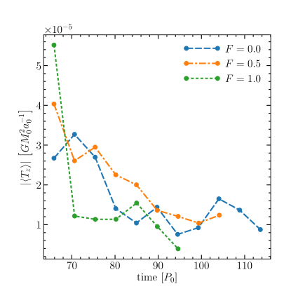
Figure 13: Total integrated torque evolution measured during the ‘forked’ simulations. Points correspond to the average of the profiles shown in Fig. 12. The light blue line shows the evolution of the $F=0.0$ distribution, the orange line is the $F=0.5$ distribution, and the green lines is the $F=1.0$ distribution. This shows that the slow relaxation of the discs translates into decreasing gravitational influence.

Using these simulations we measure how the total integrated torque profile evolves in time for each of the discs, as we show in Fig. 12. Similar to Fig. 10, each line is the radial profile of the torque’s $z$ component averaged over 5 binary orbital periods. From this figure it is clear that the gravitational influence of each disc tends to decrease as time passes (from lighter to darker lines), showing that the measured evolution driven by torques is still transient and not a long term effect. For the co-rotating circumbinary discs (left and middle plots of Fig. 12) the shape of the profile remains rather unperturbed, which means that the discs evolve smoothly. This is not the case for the counter-rotating disc (right plot of Fig. 12), where we observe strong changes in the profile outside the corotation radius. This occurs because this circumbinary ring-like structure has little angular momentum, and hence it can be perturbed much more easily by gaseous clumps and streams reaching the binary from previous interactions. Nevertheless, the profile inside the binary’s orbit remains roughly unperturbed, just decreasing its strength with time. Consequently, the evolution of the torque profiles displayed in Fig. 12 clearly shows the transient nature of the large torques found in our simulations.

The relaxation of the discs becomes even more apparent when we compute the total $z$ torque (averaged over five orbits) as a function of time, as shown in Fig. 13. The trend is clear: the net gravitational effect of the discs decreases in time. This damping of the torque is occurring somewhat slowly in our simulations, but this is likely due to the fact that we are not including any source of viscosity on top of the artificial term to capture shocks. This artificial viscosity acts as an effective viscosity within the disc, but is typically very small (Lodato & Price 2010). We would expect these discs to relax much faster with a more realistic prescription for the viscosity.

Nonetheless, we can use the formalism presented in Roedig & Sesana (2014) to make an order of magnitude estimation of total effect of such discs in the binary orbit. If we take the simple assumption that the gravitational torques evolve only the semimajor axis, we can write

$$\frac{\dot{a}}{a_{0}}\sim\frac{2T_{z}}{L_{z,0}},$$ (8)

where $L_{z,0}=0.25M_{0}\sqrt{GM_{0}a_{0}}$ for our equal-mass and circular binary. By taking an average torque of $T_{z}\sim 10^{-5}$, this expression yields

$$\dot{a}\sim-8\times 10^{-5}a_{0}\Omega_{0},$$ (9)

which over the $\approx 900$ dynamical times that span our 50k simulations translates onto a total evolution of

$$\Delta a_{\rm disc}\sim 7\times 10^{-2}a_{0}.$$ (10)

Comparing this value with the final $\Delta a$ of each distribution (Table 1), we find that corresponds to $\sim$40% for the $F=0.0$, $\sim$20% for the $F=0.5$, and $\sim$10% for the $F=1.0$ distribution. Even though this seems to indicate that the circumbinary structures contribute with an important fraction of the evolution, we arrived to this number by considering the presence of the circumbinary disc during the entirety of the run, which is certainly not true. As a matter of fact, these discs arose after the arrival of the 10th cloud, and only the one from the $F=0.0$ distribution survives the interaction during the rest of the simulation, the other two are destroyed by the interaction following a few clouds (Maureira-Fredes et al. 2018). Consequently, this estimate demonstrates that the extraction of angular momentum via gravitational torques from a circumbinary disc is subdominant with respect to capture and accretion of material, particularly for the $F=0.5$ and $F=1.0$ distributions, where these structures are unlikely to survive.

4 Additional run: the effects of shorter arrival times

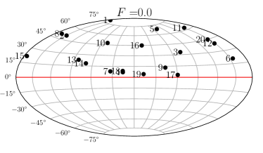
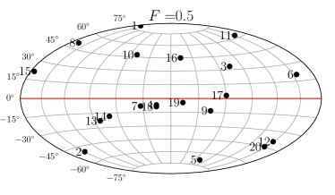
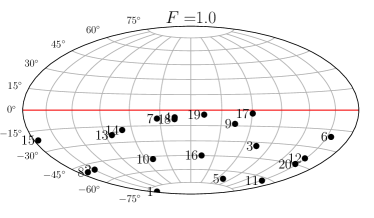
Figure 14: Compilation of the initial conditions for RunA. This is similar to the distributions shown in Figs. 1 and 2, where on the three top plots we display the cloud’s angular momentum orientations for the different levels of anisotropy, while the bottom plot shows the distribution of pericentre distances and the as a function of the time of inclusion.

Due to the stochasticity intrinsic to the low number of injected clouds, significant scatter in the MBHB evolution can be expected in different realisations of the interacting cloud population. We thus analysed a second suite of simulations, corresponding to RunA in Maureira-Fredes et al. (2018). Initial conditions for this set of runs are shown in Fig. 14. As described in Maureira-Fredes et al. (2018), due to computational limitations we were unable to achieve the 20th cloud for all the $F$ distributions, and we integrated RunA $F=0.0$ up to cloud 15, RunA $F=0.5$ up to cloud 22 and RunA $F=0.0$ up to cloud 12. To facilitate the comparison with the previous results, here we present only up to cloud 20.

Besides featuring a different random seed for the generation of initial pericentre and angular momentum distributions, this set of simulations is characterised by a much shorter average elapsed time in between clouds. This can be clearly seen by comparing the time of the final cloud ($t_{\rm 20th}$) in both runs – while in RunB the the 20th cloud is introduced at around $t_{\rm 20th}\approx$120 $P_{0}$ (Fig. 2), for RunA this time is $t_{\rm 20th}\approx$60 $P_{0}$ (Fig. 14, bottom plot). This translates onto an average time difference a factor of 2 smaller for the latter.

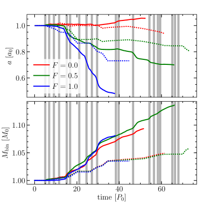
Figure 15: Same as Fig. 5, but for RunA.

One of the most significant results presented in the previous section is the deviation of the binary evolution from what predicted by the single cloud model. A difference that clearly shows the effects of the non-accreted material, which was not taken into account in that model. We repeated the analysis for RunA, results are shown in Fig. 15. Most of the conclusions drawn for RunB also apply to this case. For instance, although the the single cloud model is able to roughly reproduce the evolution driven by interaction with the first few clouds, it consistently underestimates the cumulative binary shrinking as further clouds are added to the system. A striking difference between the actual evolution and the prediction of the single cloud model is observed in the $F=0.0$ case, in which the binary slightly expands instead of shrinking its orbit.

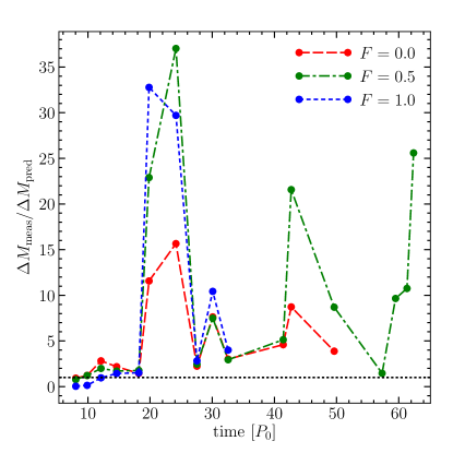
Figure 16: Same as Fig. 7, but for RunA.

Similar to RunB, we observe that the total accreted mass measured in the multicloud simulation is about a factor 3 larger than the value predicted by the single cloud models. Consequently, the dominant effect of the surrounding gas on RunA also appears to be the enhanced accretion caused by the interaction with the new incoming clouds. To quantify this increase in accretion, we directly compare figures predicted by the single cloud model with those measured from the simulations in Fig. 16. This comparison clearly shows that the single cloud model underestimates the accreted mass onto the binary after the first few clouds even more consistently than in RunB. This occurs because the typically shorter times between events does not allow for material to settle into a disc. This is one of the main results shown in Maureira-Fredes et al. (2018) – in order for the gas to settle into a more stable circumbinary configuration it needs to gain some angular momentum, which takes a few binary orbits. When clouds interact frequently with the binary, new incoming clouds strongly perturb the surrounding gas structures, prompting a lot of accretion onto the binary. In agreement with RunB, this is the main source of deviation with respect to the single cloud predictions shown in Fig. 15.

Figure 17: Same as Fig. 10, but for the circumbinary structures observed during RunA. Please note that the circumbinary dics responsible for the represented torques were identified on different times depending on the distributions: after the 12th cloud for $F=0.0$, 16th for $F=0.5$ and 10th for $F=1.0$.

Despite the higher infall rate of clouds in RunA, we do observe also the formation of somewhat coplanar circumbinary discs, albeit they get continuously destroyed by the interaction with new incoming gas (Maureira-Fredes et al. 2018). Opposite to RunB, those discs are less prominent and on average much lighter. Nonetheless, we can compute the gravitational influence of these circumbinary structures through the torque that the gas exerts on the binary. The differential and integrated radial torque profiles are shown in Fig. 17.

Compared to the profiles shown in Fig. 10 we observe similar features, confirming the robustness of the dynamics against different realisations of the interacting cloud population. In particular, in the $F=0.0$ and $F=0.5$ runs, material outside the corotation radius is transporting some of the binary’s angular momentum outwards via gravitational slingshot, while for the $F=1.0$ distribution all the negative torques come from the material inside the binary orbit.

Interestingly, in the $F=0.0$ simulation the positive torque inside the corotation radius is larger than the outwards torque, which implies that the net effect of the gravitational forces is to add momentum to the binary, expanding its orbit. This is likely why the final semimajor axis during this simulation is larger than the initial value, in contrast to the predicted evolution which is a slight shrinking of the orbit. The continuous disruption of arising structures due to frequent infall of clouds, supplies a larger amount of gas inside the binary’s orbit, enhancing these positive torques. If the accretion events were to stop, or decrease in frequency, the surviving material would settle into a circumbinary disc, and as the binary opens up a cavity, gravitational slingshot of gaseous streams would becomes the dominant effect, shrinking its semimajor axis.

Overall, the main conclusions found in the previous section apply to this run. The dominant effect of the non-accreted material on the binary evolution comes from the enhanced accretion produced by stream interactions. Due to the higher infalling rate we find that is even more difficult to build massive and stable circumbinary structures (Maureira-Fredes et al. 2018), which further decreases the influence of the angular momentum transport by gravitational torques. The net result is that the dynamics of the system is mostly driven by capture and accretion of mass, which has the interesting effect of making the evolution of the binary even more sensitive to the details of the cloud distributions. In general, for isotropic or counter-rotating distributions, the mutual partial cancellation of the MBHB and the accreted gas angular momenta accelerates the binary shrinking, driving the binary to a faster coalescence. In the co-rotating case, the resulting binary evolution depends on a subtle balance between accreted mass and angular momentum, with the net effect that the MBHB can also slightly expand. A longer simulation is required to confirm whether the expansion seen in RunA $F=0.0$ is only transient or if it holds in the long term.

5 Summary and discussion

On this paper we have introduced a new suite of simulations to study the evolution of a binary embedded in a turbulent environment, where we expect several gaseous clumps to infall and dynamically interact with the binary. The main goal was to overcome the limitations of the Monte Carlo evolution presented in Paper II by directly modelling the interaction of a MBHB with a sequence of incoherent accretion events. These models combine the ‘discrete’ evolution due to the prompt interaction of each individual cloud, with the secular torques exerted by the left-over gas. The latter could not be numerically resolved in the single cloud models, but could have a role on the dynamics of both gas and binary.

In order to directly compare with the results of the Monte Carlo evolution of Paper II, the cloud orbits where sampled using the same probability density functions. In particular, we have used the $F$-distributions for the angular momentum orientation which are an indication of the anisotropy levels in the surrounding medium. These distributions have been linked to the morphological and kinematical properties of the host galaxy (Sesana et al. 2014).

Our main findings can be summarised as follows:

1. The MBHB angular momentum evolution follows the injection of momentum in the form of clouds. That is, the binary monotonically increases its angular momentum (even though it still shrinks) in the $F=0.0$ model where each new cloud adds to the total momentum budget, while continuously decreasing for $F=1.0$ where the opposite occurs. This is consistent with the scenario where the orbital evolution is dominated by direct exchange of angular momentum through capture and accretion, as demonstrated by the single cloud simulations in Paper II.

2. The binary exhibits an almost identical orbital evolution at every investigated resolution. This is because the dynamical evolution of the system is dominated by capture and gravitational slingshot, which are properly resolved even with a low number of particles.

3. The largest differences are present in the eccentricity evolution due to typically low values ($e\lesssim 0.02$), making it much more sensitive to noise. Because of this, we focused the analysis on the semimajor axis and mass evolution, considering that the binary remains circular throughout the whole simulation.

4. Also concordant with the single cloud simulations, the evolution of the semimajor axis is strongly dependent on the distribution of the infalling gas, being fastest when it features more counter-rotating clouds. Conversely, the binary mass evolution is roughly independent of the cloud distribution during most of the interaction.

5. By directly comparing the observed binary evolution with a semi-analytical model constructed on the basis of the single cloud simulations, we found that accretion onto the MBHB increases considerably (by about a factor of three). This occurs because new incoming material is able to drag inward a fraction of the surrounding gas leftover by previous accretion events.

6. Enhanced accretion has a strong impact on the evolution of the binary. Because of angular momentum cancellation with a larger mass of infalling gas, the binary evolution is accelerated in the isotropic and counter-rotating cases (by 20-to-50% and a factor $\approx$2, respectively, see Figs. 5 and 15). In the co-rotating case, the evolution depends on a fine balance of mass and angular momentum accretion, and can lead, at least temporarily, to the expansion of the binary semimajor axis.

7. In the $F=0.0$ and $F=0.5$ models we observe the intermittent formation of well-defined, coplanar and co-rotating circumbinary discs. The discs present well-known features, in particular, a cavity located at $r\approx 2a$ which is maintained by the resonances of the orbiting gas with the binary’s gravitational potential.

8. Similarly, we observed the formation of intermittent coplanar and counter-rotating circumbinary discs in the $F=1.0$ model. Due to the absence of resonances, in this case the gas is able to orbit much closer to the binary.

9. By computing the gravitational torques exerted by the surrounding gas, we have shown that these discs are able to transport some of the binary’s angular momentum via gaseous streams that are slingshotted away once they get close to the MBHs. This process can continue shrinking the binary orbit in the absence of new impacting clouds. However, due to the low mass of these discs, their effect on the binary orbital decay is subdominant with respect to the capture and subsequent accretion of the incoherent material deposited by clouds in the vicinity of the MBHB.

An interesting case is the isotropic scenario $F=0.5$ where the total angular momentum brought by the gas is close to zero, at least after a significant number of clouds. In this scenario, the intersection of highly misaligned streams tend to effectively cancel angular momentum, forcing material to plunge onto the binary. Therefore, we do not expect a steady circumbinary disc to survive under these conditions. Following a sequence of 10 clouds, however, there is a clear circumbinary structure rising from the non-accreted material, which is already producing a noticeable effect on the binary orbit. This implies that the formation of circumbinary discs is a relevant process even for the $F=0.5$ model, even if these discs are transient and with negligible self-gravity. One of the assumptions of the Monte Carlo models presented in Paper II is that there is no circumbinary disc during the isotropic scenario due to the low total angular momentum of the gas. Our results clearly show the inadequacy of this assumption. This occurs because corotating material is able to gain more angular momentum via resonances and gravitational slingshot compared to counter-rotating gas, thus forming meta-stable disc-like configurations.

At this point, it is important to stress that our simulations are subject to a number of limitations, that we now briefly consider. The mass of the circumbinary discs intermittently forming throughout the simulations is small compared to the binary and hence their self-gravity is negligible (Maureira-Fredes et al. 2018). In this situation the outwards transport of angular momentum throughout the disc will occur through an unresolved viscosity (see e.g. Syer & Clarke 1995; Ivanov et al. 1999; Ragusa et al. 2016). For geometrically thin and optically thick discs, such viscosity is commonly parametrised using the $\alpha$-disc model (Shakura & Sunyaev 1973), where $\alpha$ represents the strength of the internal viscous stresses. In our simulations, however, the only source of viscosity is the artificial term introduced to capture shocks, hence the transport of angular momentum throughout the disc is likely not adequately modelled. Additionally, the evolution of the binary-disc system might be affected by the simple thermodynamics adopted in these models. As discussed in Roedig et al. (2012), the morphology of the streaming gas has a major impact in the binary evolution and the structure of the surrounding disc, thus it is directly influenced by the gas thermodynamics. Moreover, Tang et al. (2017) using 2D hydrodynamical simulations of circumbinary accretion discs found that the torques are sensitive to the sink prescription: slower sinks result in more gas accumulating near the MBHs, driving the binary to merge more rapidly. Nevertheless, all these effects become relevant for the long-term evolution of a MBHB embedded in a circumbinary disc, where torques mediated by resonances play an important role in the evolution of the system. Conversely, during the infall of a sequence of clouds, the relevant mechanisms driving the binary’s orbital response are almost purely dynamical, namely, gas capture and gravitational slingshot, which are well resolved with these models. Therefore, a more physical treatment for the viscosity, thermodynamics and accretion in required only if one wants to resolve the long-term evolution of the MBHB surrounded by a circumbinary disc arising in the aftermath of the accretion events.

Even though the self-gravity of the discs presented in this paper is negligible, it could certainly play a role in the evolution of the system depending on the cloud distribution. If the leftover material were to settle onto a well defined circumbinary structure (which depends on the frequency of events, see Maureira-Fredes et al. 2018), it could eventually fragment to form stars, as demonstrated by Dunhill et al. (2014), especially for higher cloud masses. Based on our results, we expect fragmentation on the left-over gas to marginally decrease the effects of the infalling clouds, mainly because it would reduce the amount of available material to interact with the new incoming clouds. Nonetheless, for these near-radial clouds, the transient effect during the first impact is still efficient to evolve the binary (Paper II). Furthermore, a fragmenting circumbinary disc can continue shrinking the binary orbit by sending stars into the loss-cone, as shown by Amaro-Seoane et al. (2013), although the efficiency drops considerably with respect to a similar, non-fragmented disc.

Another delicate point is the simplified treatment of accretion, whereby every bound particle entering the sink radius is added to the MBHs. When scaled to our fiducial physical model ($M_{\rm bin}=10^{6}M_{\odot}$, $a_{0}=0.2$ pc), this results in sparse episodes of highly super-Eddington accretion. The exact fate of the gas during this ‘accretion spikes’ is uncertain. The extremely high density of the accretion flow might cause photon diffusion timescale to be longer than the accretion timescale, thus advecting photons into the MBHs, in turn allowing super-Eddington accretion rates. Conversely, radiation pressure in the proximity of the MBHs might cause copious mass loss through powerful winds, significantly decreasing the amount of accretion. As noticed in Paper II, the exchange of angular momentum is mostly mediated by capture of gas in bound orbits around the individual MBHs rather than subsequent accretion. Even assuming that the majority of the gas is accelerated away in form of isotropic winds, the evolution of the binary is affected at a level of 20-30%. This conclusion, however, does not take into account the interaction of the outgoing wind with the infalling clouds. If winds are isotropic and strong enough to clear the infalling gas on large scales, this would quench the supply of material onto the MBHB, eventually stalling the binary. A proper investigation of this potential issue requires the implementation of a suitable feedback prescription, and we plan to explore this in future work.

A somewhat different aspect that might be impacting our results is the resolution elements of the individual clouds. For instance, in their simulations Dunhill et al. (2015) found that the dynamics of gaseous streams going through the cavity is resolution dependent. As discussed above, the streams play an important role transporting angular momentum once the circumbinary disc has formed, thus the late evolution measured using the lower resolution runs is likely affected by this issue. In fact, we find some differences with resolution in the gravitational torques studied in §3. For the $F=0.0$ and $F=0.5$ distributions the differences are relatively small, $\sim$16% and $\sim$6%, respectively, between the 50k and 1m models. On the other hand, for the $F=1.0$ distribution, we found up to a factor of $\sim$2 difference between the 50k and 500k resolutions. These larger differences are likely because the material close to the binary self-interacts more strongly in the retrograde case compared with the other two distributions, since the absence of resonances does not allow the gas to gain angular momentum. In this scenario, the interaction of the different gas streams determines the amount of material in the circumbinary disc, and this is more sensitive to the resolution of the clouds. Since we are not observing strong resolution dependence in the binary semimajor axis, these effects are still sub-dominant with respect to the accretion of gas. Consequently, resolution would become much more important for low infall frequency of clouds, where the material is expected to settle into a more ‘stable’ circumbinary disc.

Another relevant aspect that might have implications for our conclusions is the chosen mass ratio between the binary and the incoming clouds. As explained in Paper I, we based our study in the simulations presented by Bonnell & Rice (2008), where they numerically modelled the infall of a molecular cloud onto single MBHs with the goal of explaining the stellar distribution observed in our Galactic Centre. Their fiducial model is a $10^{4}M_{\odot}$ cloud infalling onto a $10^{6}M_{\odot}$ black hole, hence we adopted the same mass ratio in our simulations. Based on the numerical studies of multiphase gas in the interstellar medium (e.g. Hobbs et al. 2011; Gaspari et al. 2013, 2015; Fiacconi et al. 2018), we expect the orbital parameters and internal properties of the cold clumps to be independent on the mass of the central object, as they are determined by large-scale physical processes in the galaxy such as turbulence, rotation, cooling, heating, among others. So, in principle, the relative effect that each cloud has on the binary evolution should scale linearly with the MBHB-to-cloud mass ratio. We also deliberately chose identical clouds infalling onto the MBHBs, in order to single out the impact of their different orbits. This is clearly not a realistic setup, as a distribution of clump masses is expected. More sophisticated initial conditions can be derived from numerical models of realistic galaxies that include all the relevant physical mechanisms. We plan to extend our simulation setup in this direction in future work.

Despite the aforementioned limitations, the results exhibited in this paper suggest that the secular effects of the left-over material further increase the efficiency of the incoherent infalling clouds to bring the MBHs towards coalescence respect to a scenario that only considers the evolution during the prompt accretion phase, as the one presented in Paper II. Consequently, provided there is a reasonable rate of events, these models confirm that infalling clouds present a viable mechanism to efficiently merge these binaries within less then a Gyr.

References

- Alig et al. (2011) Alig C., Burkert A., Johansson P. H., Schartmann M., 2011, MNRAS, 412, 469
- Amaro-Seoane et al. (2013) Amaro-Seoane P., Brem P., Cuadra J., 2013, ApJ, 764, 14
- Amaro-Seoane et al. (2017) Amaro-Seoane P., et al., 2017, preprint, (arXiv:1702.00786)
- Arca Sedda et al. (2017) Arca Sedda M., Berczik P., Capuzzo-Dolcetta R., Fragione G., Sobolenko M., Spurzem R., 2017, preprint, (arXiv:1712.05810)
- Armitage & Natarajan (2005) Armitage P. J., Natarajan P., 2005, ApJ, 634, 921
- Artymowicz & Lubow (1994) Artymowicz P., Lubow S. H., 1994, ApJ, 421, 651
- Artymowicz & Lubow (1996) Artymowicz P., Lubow S. H., 1996, ApJ, 467, L77
- Barnes & Hernquist (1992) Barnes J. E., Hernquist L., 1992, ARA&A, 30, 705
- Begelman et al. (1980) Begelman M. C., Blandford R. D., Rees M. J., 1980, Nature, 287, 307
- Binney & Tremaine (2008) Binney J., Tremaine S., 2008, Galactic Dynamics: Second Edition. Princeton University Press
- Bondi (1952) Bondi H., 1952, MNRAS, 112, 195
- Bonnell & Rice (2008) Bonnell I. A., Rice W. K. M., 2008, Science, 321, 1060
- Bortolas et al. (2018) Bortolas E., Mapelli M., Spera M., 2018, MNRAS, 474, 1054
- Combes et al. (2007) Combes F., Young L. M., Bureau M., 2007, MNRAS, 377, 1795
- Consortium et al. (2013) Consortium T. e., et al., 2013, arXiv:1305.5720,
- Cuadra et al. (2006) Cuadra J., Nayakshin S., Springel V., Di Matteo T., 2006, MNRAS, 366, 358
- Cuadra et al. (2009) Cuadra J., Armitage P. J., Alexander R. D., Begelman M. C., 2009, MNRAS, 393, 1423
- D’Orazio et al. (2013) D’Orazio D. J., Haiman Z., MacFadyen A., 2013, MNRAS, 436, 2997
- D’Orazio et al. (2015) D’Orazio D. J., Haiman Z., Duffell P., Farris B. D., MacFadyen A. I., 2015, MNRAS, 452, 2540
- Dabringhausen et al. (2008) Dabringhausen J., Hilker M., Kroupa P., 2008, MNRAS, 386, 864
- David et al. (2014) David L. P., et al., 2014, ApJ, 792, 94
- Dunhill et al. (2014) Dunhill A. C., Alexander R. D., Nixon C. J., King A. R., 2014, MNRAS, 445, 2285
- Dunhill et al. (2015) Dunhill A. C., Cuadra J., Dougados C., 2015, MNRAS, 448, 3545
- Escala et al. (2004) Escala A., Larson R. B., Coppi P. S., Mardones D., 2004, ApJ, 607, 765
- Escala et al. (2005) Escala A., Larson R. B., Coppi P. S., Mardones D., 2005, ApJ, 630, 152
- Farris et al. (2015a) Farris B. D., Duffell P., MacFadyen A. I., Haiman Z., 2015a, MNRAS, 446, L36
- Farris et al. (2015b) Farris B. D., Duffell P., MacFadyen A. I., Haiman Z., 2015b, MNRAS, 447, L80
- Ferrarese & Merritt (2000) Ferrarese L., Merritt D., 2000, ApJ, 539, L9
- Fiacconi et al. (2013) Fiacconi D., Mayer L., Roškar R., Colpi M., 2013, ApJ, 777, L14
- Fiacconi et al. (2018) Fiacconi D., Sijacki D., Pringle J. E., 2018, MNRAS,
- Gaburov et al. (2012) Gaburov E., Johansen A., Levin Y., 2012, ApJ, 758, 103
- Gaspari & Sa̧dowski (2017) Gaspari M., Sa̧dowski A., 2017, ApJ, 837, 149
- Gaspari et al. (2012) Gaspari M., Ruszkowski M., Sharma P., 2012, ApJ, 746, 94
- Gaspari et al. (2013) Gaspari M., Ruszkowski M., Oh S. P., 2013, MNRAS, 432, 3401
- Gaspari et al. (2015) Gaspari M., Brighenti F., Temi P., 2015, A&A, 579, A62
- Gaspari et al. (2017) Gaspari M., Temi P., Brighenti F., 2017, MNRAS, 466, 677
- Gaspari et al. (2018) Gaspari M., et al., 2018, ApJ, 854, 167
- Gebhardt et al. (2000) Gebhardt K., et al., 2000, ApJ, 539, L13
- Goicovic et al. (2016) Goicovic F. G., Cuadra J., Sesana A., Stasyszyn F., Amaro-Seoane P., Tanaka T. L., 2016, MNRAS, 455, 1989
- Goicovic et al. (2017) Goicovic F. G., Sesana A., Cuadra J., Stasyszyn F., 2017, MNRAS, 472, 514
- Haiman et al. (2009) Haiman Z., Kocsis B., Menou K., 2009, ApJ, 700, 1952
- Hernquist (1990) Hernquist L., 1990, ApJ, 356, 359
- Hobbs & Nayakshin (2009) Hobbs A., Nayakshin S., 2009, MNRAS, 394, 191
- Hobbs et al. (2011) Hobbs A., Nayakshin S., Power C., King A., 2011, MNRAS, 413, 2633
- Hopkins & Quataert (2011) Hopkins P. F., Quataert E., 2011, MNRAS, 415, 1027
- Ivanov et al. (1999) Ivanov P. B., Papaloizou J. C. B., Polnarev A. G., 1999, MNRAS, 307, 79
- Jahnke & Macciò (2011) Jahnke K., Macciò A. V., 2011, ApJ, 734, 92
- Kelly & Shen (2013) Kelly B. C., Shen Y., 2013, ApJ, 764, 45
- King & Pringle (2006) King A. R., Pringle J. E., 2006, MNRAS, 373, L90
- King & Pringle (2007) King A. R., Pringle J. E., 2007, MNRAS, 377, L25
- Kocsis et al. (2012) Kocsis B., Haiman Z., Loeb A., 2012, MNRAS, 427, 2680
- Kormendy & Ho (2013) Kormendy J., Ho L. C., 2013, ARA&A, 51, 511
- Lodato & Price (2010) Lodato G., Price D. J., 2010, MNRAS, 405, 1212
- Lodato et al. (2009) Lodato G., Nayakshin S., King A. R., Pringle J. E., 2009, MNRAS, 398, 1392
- Lu et al. (2009) Lu J. R., Ghez A. M., Hornstein S. D., Morris M. R., Becklin E. E., Matthews K., 2009, ApJ, 690, 1463
- Lucas et al. (2013) Lucas W. E., Bonnell I. A., Davies M. B., Rice W. K. M., 2013, MNRAS, 433, 353
- Lupi et al. (2015) Lupi A., Haardt F., Dotti M., Colpi M., 2015, MNRAS, 453, 3437
- MacFadyen & Milosavljević (2008) MacFadyen A. I., Milosavljević M., 2008, ApJ, 672, 83
- Magorrian et al. (1998) Magorrian J., et al., 1998, AJ, 115, 2285
- Mapelli & Trani (2016) Mapelli M., Trani A. A., 2016, A&A, 585, A161
- Mapelli et al. (2012) Mapelli M., Hayfield T., Mayer L., Wadsley J., 2012, ApJ, 749, 168
- Masunaga & Inutsuka (2000) Masunaga H., Inutsuka S.-i., 2000, ApJ, 531, 350
- Maureira-Fredes et al. (2018) Maureira-Fredes C., Goicovic F. G., Amaro-Seoane P., Sesana A., 2018, preprint, (arXiv:1801.06179)
- Mayer et al. (2007) Mayer L., Kazantzidis S., Madau P., Colpi M., Quinn T., Wadsley J., 2007, Science, 316, 1874
- McNamara et al. (2014) McNamara B. R., et al., 2014, ApJ, 785, 44
- Miranda et al. (2017) Miranda R., Muñoz D. J., Lai D., 2017, MNRAS, 466, 1170
- Muñoz & Lai (2016) Muñoz D. J., Lai D., 2016, ApJ, 827, 43
- Nayakshin & King (2007) Nayakshin S., King A., 2007, arXiv:0705.1686,
- Nayakshin et al. (2012) Nayakshin S., Power C., King A. R., 2012, ApJ, 753, 15
- Nixon & Lubow (2015) Nixon C., Lubow S. H., 2015, MNRAS, 448, 3472
- Nixon et al. (2011) Nixon C. J., Cossins P. J., King A. R., Pringle J. E., 2011, MNRAS, 412, 1591
- Paumard et al. (2006) Paumard T., et al., 2006, ApJ, 643, 1011
- Ragusa et al. (2016) Ragusa E., Lodato G., Price D. J., 2016, MNRAS, 460, 1243
- Roedig & Sesana (2014) Roedig C., Sesana A., 2014, MNRAS, 439, 3476
- Roedig et al. (2011) Roedig C., Dotti M., Sesana A., Cuadra J., Colpi M., 2011, MNRAS, 415, 3033
- Roedig et al. (2012) Roedig C., Sesana A., Dotti M., Cuadra J., Amaro-Seoane P., Haardt F., 2012, A&A, 545, A127
- Roškar et al. (2015) Roškar R., Fiacconi D., Mayer L., Kazantzidis S., Quinn T. R., Wadsley J., 2015, MNRAS, 449, 494
- Russell et al. (2014) Russell H. R., et al., 2014, ApJ, 784, 78
- Sanders & Mirabel (1996) Sanders D. B., Mirabel I. F., 1996, ARA&A, 34, 749
- Sesana et al. (2014) Sesana A., Barausse E., Dotti M., Rossi E. M., 2014, ApJ, 794, 104
- Shakura & Sunyaev (1973) Shakura N. I., Sunyaev R. A., 1973, A&A, 24, 337
- Shi & Krolik (2015) Shi J.-M., Krolik J. H., 2015, ApJ, 807, 131
- Shi et al. (2012) Shi J.-M., Krolik J. H., Lubow S. H., Hawley J. F., 2012, ApJ, 749, 118
- Springel (2005) Springel V., 2005, MNRAS, 364, 1105
- Syer & Clarke (1995) Syer D., Clarke C. J., 1995, MNRAS, 277, 758
- Tang et al. (2017) Tang Y., MacFadyen A., Haiman Z., 2017, MNRAS, 469, 4258
- Tang et al. (2018) Tang Y., Haiman Z., MacFadyen A., 2018, MNRAS, 476, 2249
- Temi et al. (2018) Temi P., Amblard A., Gitti M., Brighenti F., Gaspari M., Mathews W. G., David L., 2018, ApJ, 858, 17
- Tremblay et al. (2016) Tremblay G. R., et al., 2016, Nature, 534, 218
- White & Rees (1978) White S. D. M., Rees M. J., 1978, MNRAS, 183, 341
- del Valle et al. (2015) del Valle L., Escala A., Maureira-Fredes C., Molina J., Cuadra J., Amaro-Seoane P., 2015, ApJ, 811, 59