The existence of horizontal envelopes in the 3D-Heisenberg group

Abstract

By using the support function on the $xy$-plane, we show the necessary and sufficient conditions for the existence of envelopes of horizontal lines in the 3D-Heisenberg group. A method to construct horizontal envelopes from the given ones is also derived, and we classify the solutions satisfying the construction.

1 Introduction

Given a family of lines in $\mathbb{R}^{2}$. The envelope of the family of lines $F(\lambda,x,y)$, depending on the parameter $\lambda$, is defined to be a curve on which every line in the family contacts exactly at one point. A simple example is to find the envelope of the family of lines $F(\lambda,x,y)=(1-\lambda)x+\lambda y-\lambda(1-\lambda)=0$ for $\lambda\in[0,1]$ and $(x,y)\in[0,1]\times[0,1]$. Consider the system of differential equations

$$\left\{\begin{array}[]{rl}F(\lambda,x,y)&=0,\\ \frac{\partial F(\lambda,x,y)}{\partial\lambda}&=0.\end{array}\right.$$ (3)

The second equation helps us find $\lambda$ in terms of $x,y$, and substitute $\lambda$ into the first equation to have the envelope

$$x^{2}+y^{2}-2xy-2x-2y+1=0.$$ (4)

Note that there are totally three variables $\lambda,x,y$, two equations in the system of differential equations (3), and hence one gets the solution (4) which is a one-dimensional curve in $\mathbb{R}^{2}$. One of applications in Economics to finding the envelopes is the Envelope Theorem which is related to gain the optimal production functions for given input and output prices [2, 7]. Recently the theorem has been generalized to the functions of multivariables with non-differentiability condition [4]. In general, it is impossible to seek the envelope of a family of lines in the higher dimensional Euclidean spaces $\mathbb{R}^{n}$ for $n\geq 3$ due to the over-determined system of differential equations similar to (3) (Sec. 26, Chapter 2 [3]). However, by considering the $3$-dimensional Heisenberg group $\mathbb{H}_{1}$ as a sub-Riemannian manifold, the horizontal envelopes can be obtained by a family of horizontal lines. In this notes we will study the problem of existence for horizontal envelopes in $\mathbb{H}_{1}$.

We recall some terminologies for our purpose. For more details about the Heisenberg groups, we refer the readers to [1, 6, 8, 9]. The $3$-dimensional Heisenberg group $\mathbb{H}_{1}$ is the Lie group $(\mathbb{R}^{3},\star)$, where the group operation $\star$ is defined, for any point $(x,y,z)$, $(x^{\prime},y^{\prime},z^{\prime})\in\mathbb{R}^{3}$, by

$$(x,y,z)\star(x^{\prime},y^{\prime},z^{\prime})=(x+x^{\prime},y+y^{\prime},z+z^{\prime}+yx^{\prime}-xy^{\prime}).$$

For $p\in\mathbb{H}^{1}$, the left translation by $p$ is the diffeomorphism $L_{p}(q):=p\star q$. A basis of left invariant vector fields (i.e., invariant by any left translation) is given by

$$\mathring{e}_{1}(p):=\frac{\partial}{\partial x}+y\frac{\partial}{\partial z},\ \mathring{e}_{2}(p):=\frac{\partial}{\partial y}-x\frac{\partial}{\partial z},\ T(p):=(0,0,1).$$

The horizontal distribution (or contact plane $\xi_{p}$ at any point $p\in\mathbb{H}^{1})$ is the smooth planar one generated by $\mathring{e}_{1}(p)$ and $\mathring{e}_{2}(p)$. We shall consider on $\mathbb{H}_{1}$ the (left invariant) Riemannian $g:=\langle.,.\rangle$ so that $\{\mathring{e}_{1},\mathring{e}_{2},T\}$ is an orthonormal basis in the Lie algebra of $\mathbb{H}^{1}$. The endomorphism $J:\mathbb{H}_{1}\rightarrow\mathbb{H}_{1}$ is defined such that $J(\mathring{e}_{1})=\mathring{e}_{2}$, $J(\mathring{e}_{2})=-\mathring{e}_{1}$, $J(T)=0$ and $J^{2}=-1$.

A curve $\gamma:I\subset\mathbb{R}\rightarrow\mathbb{H}_{1}$ is called horizontal (or Legendrian) if its tangent at any point on the curve is on the contact plane. More precise, if we write the curve in the coordinates $\gamma:=(x,y,z)$ with the tangent vector $\gamma^{\prime}=(x^{\prime},y^{\prime},z^{\prime})=x^{\prime}\mathring{e}_{1}(\gamma)+y^{\prime}\mathring{e}_{2}(\gamma)+T(z^{\prime}-x^{\prime}y+xy^{\prime})$, then the curve $\gamma$ is horizontal if and only if

$$z^{\prime}-x^{\prime}y+xy^{\prime}=0,$$ (5)

where the prime ^′ denotes the derivative with respect to the parameter of the curve. The velocity $\gamma^{\prime}$ has the natural decomposition

$$\gamma^{\prime}=\gamma^{\prime}_{\xi}+\gamma^{\prime}_{T},$$

where $\gamma^{\prime}_{\xi}$ (resp. $\gamma^{\prime}_{T}$) is the orthogonal projection of $\gamma^{\prime}$ on $\xi$ along $T$ (resp. on $T$ along $\xi$) with respect to the metric $g$. Recall that a horizontally regular curve is a parametrized curve $\gamma(t)$ such that $\gamma^{\prime}_{\xi}(u)\neq 0$ for all $u\in I$ (Definition 1.1 [1]). Also, in Proposition 4.1 [1], we show that any horizontally regular curve can be uniquely reparametrized by horizontal arc-length $s$, up to a constant, such that $|\gamma^{\prime}_{\xi}(s)|=1$ for all $s$, and called the curve being with horizontal unit-speed. Moreover, two geometric quantities for horizontally regular curves parametrized by arc-length, the p-curvature $k(s)$ and the contact normality $\tau(s)$, are defined by

$$k(s) :=\langle\frac{d\gamma^{\prime}(s)}{ds},J\gamma^{\prime}(s)\rangle,$$

$$\tau(s) :=\langle\gamma^{\prime}(s),T\rangle,$$

which are invariant under pseudo-hermitian transformations of horizontally regular curves (Section 4, [1]). Note that $k(s)$ is analogous to the curvature of the curve in the Euclidean space $\mathbb{R}^{3}$, while $\tau(s)$ measures how far the curve is from being horizontal. When the curve $\gamma(u)$ is parametrized by arbitrary parameter $u$ (not necessarily its arc-length $s$), the p-curvature is given by

$$k(u):=\frac{x^{\prime}y^{\prime\prime}-x^{\prime\prime}y^{\prime}}{\left((x^{\prime})^{2}+(y^{\prime})^{2}\right)^{3/2}}(u).$$ (6)

It is clear that a curve $\gamma(s)$ is a horizontal if and only if $\gamma(s)=\gamma_{\xi}(s)$ for all $s$. One of examples for horizonal curves is the horizontal lines which can be characterized by the following proposition.

Proposition 1.

Any horizontal line $\ell$ in $\mathbb{H}_{1}$ can be uniquely determined by three parameters $(p,\theta,t)$ for any $p\geq 0$, $\theta\in[0,2\pi]$, $t\in\mathbb{R}$. Any point on the line can be represented in the coordinates

$$\ell:\left\{\begin{array}[]{rl}x&=p\cos\theta-s\ \sin\theta,\\ y&=p\sin\theta+s\ \cos\theta,\\ z&=t-sp,\end{array}\right.$$ (10)

for all $s\in\mathbb{R}$.

When $s=0$, denote by

$$Q^{\prime}:=(x,y,z)=(p\cos\theta,p\sin\theta,t).$$ (11)

Observe that $\ell$ is a line through the point $Q^{\prime}$ with the directional vector $\sin\theta\ \mathring{e}(Q^{\prime})+\cos\theta\ \mathring{e}(Q^{\prime})$. The value $p$ actually is the value of the support function $p(\theta)$ for the projection $\pi(\ell)$ of $\ell$ on the $xy$-plane (see the proof of Proposition 1 in next section).

Inspired by the envelopes in the plane, with the assistance of contact planes in $\mathbb{H}_{1}$ we introduce the horizontal envelope tangent to a family of horizontal lines.

Definition 1.

Given a family of horizontal lines in $\mathbb{H}_{1}$. A horizontal envelope is a horizontal curve $\gamma$ such that $\gamma$ contacts with exactly one line in the family at one point.

Back to Proposition 1, $p$ actually is the distance of the projection $\pi(\ell)$ of $\ell$ onto the $xy$-plane to the origin, and $\theta$ is the angle from the $x$-axis to the line perpendicular to the projection (see Fig. 2 next section). To obtain the horizontal envelope $\gamma$, it is natural to consider $p$ as a function of $\theta$, namely, the support function $p=p(\theta)$ for the projection $\pi(\gamma)$ of the curve on the $xy$-plane. Moreover, by (11) we know that the value $t$ dominates the height of the point $Q^{\prime}$. As long as $\theta$ is fixed, the projection of $Q^{\prime}$ onto the $xy$-plane is fixed. Thus, we may consider $t$ as a function of $\theta$. Under these circumstances, the family of horizontal lines is only controlled by one parameter $\theta$, and so the following is our main theorem.

Theorem 1.

Let $p=p(\theta)\geq 0$ and $t=t(\theta)$ be $C^{1}$-functions defined on $\theta\in[0,2\pi]$ satisfying

$$t^{\prime}=(p^{\prime})^{2}-p^{2}.$$ (12)

There exists a horizontally regular curve $\gamma$ parametrized by arc-length such that the curve is the horizontal envelope of the family of horizontal lines determined by $\theta$ (and hence $p$ and $t$). In the coordinates, the envelope $\gamma=(x,y,z)$ can be represented by

$$\gamma:\left\{\begin{array}[]{rl}x(\theta)&=p(\theta)\cos\theta-p^{\prime}(\theta)\sin\theta,\\ y(\theta)&=p(\theta)\sin\theta+p^{\prime}(\theta)\cos\theta,\\ z(\theta)&=t(\theta)-p^{\prime}(\theta)p(\theta).\end{array}\right.$$ (16)

Moreover, if $p$ is a $C^{2}$-function, the $p$-curvature and the contact normality of $\gamma$ are given by $k=\frac{1}{p+p^{\prime\prime}}$ and $\tau\equiv 0$.

Since the functions $p(\theta)$ and $t(\theta)$ uniquely determine a family of horizontal lines by  Proposition 1, we say that the horizontal envelope $\gamma$ in Theorem 1 is generated by the family of horizontal lines $(p(\theta),\theta,t(\theta))$.

Remark 1.

A geodesic in $\mathbb{H}_{1}$ is a horizontally regular curve with minimal length with respect to the Carnot-Carathéodory distance. For two given points in $\mathbb{H}_{1}$ one can find, by Chow’s connectivity Theorem ([5] p. 95), a horizontal curve joining these points. Note that when $p\equiv c$, a constant function, by (10), (12), and (16), the horizontal envelope $\gamma$ generated by the family of horizontal lines $\left\{(c,\theta,t(\theta)),\ \theta\in[0,2\pi]\right\}$ is a (helix) geodesic with radius $c$; the same result occurs if $t$ is also a constant function. In particular, when $p\equiv 0$, the horizontal envelope is the line segment contained in the $z$-axis.

Besides, the reversed statement of Theorem 1 also holds for horizontal curves with ”jumping” ends.

Theorem 2.

Let $\gamma:\theta\in[0,2\pi]\mapsto(x(\theta),y(\theta),z(\theta))\in\mathbb{H}_{1}$ be a horizonal curve with finite length. Suppose $x(0)=x(2\pi)$, $y(0)=y(2\pi)$, and $z(0)\neq z(2\pi)$. Then the set of its tangent lines is uniquely determined by $p=p(\theta)\geq 0$ and $t=t(\theta)$ satisfying (12).

We introduce a method to construct horizontal envelopes.

Corollary 1.

Let $p_{i}=p_{i}(\theta)\geq 0,t_{i}=t_{i}(\theta)$ be $C^{1}$-functions defined on $[0,2\pi]$ satisfying (12) for $i=1,2$. Suppose $\gamma_{i}=(x_{i},y_{i},z_{i})$ is a horizontal envelope generated by the family of horizontal lines $(p_{i},\theta,t_{i})$ for $i=1,2$. Denote by $p=p_{1}+p_{2}$ and $t=t_{1}+t_{2}$. The curve $\gamma=(x,y,z)$ is a horizontal envelope generated by a family of horizontal lines $(p(\theta),\theta,t(\theta))$ if and only if

$$p_{1}p_{2}=p^{\prime}_{1}p^{\prime}_{2}.$$ (17)

By Corollary 1 and Remark 1, we know that if at least one of $\gamma_{1}$ or $\gamma_{2}$ is a (helix) geodesic with nonzero radius, $\gamma$ can not be a horizontal envelope.

Now we seek the classification of functions $p_{1}$, $p_{2}$ satisfying the condition $p_{1}p_{2}=p^{\prime}_{1}p^{\prime}_{2}$ in Corollary 1. Actually, for any subinterval $[a,b]\subset[0,2\pi]$ such that $p_{i}\neq 0$ and $p^{\prime}_{i}\neq 0$ for $i=1,2$, the condition (17) is equivalent to $p_{1}(\theta)=p_{1}(a)\exp\left(\int_{a}^{\theta}\frac{p_{2}(\alpha)}{p^{\prime}_{2}(\alpha)}d\alpha\right)$ for any $\theta\in[a,b]$. In addition, if $p_{i}(\theta_{i})=0$ for some $\theta_{i}\in[0,2\pi]$, we may move the horizontal envelope $\gamma$ by a left translation such that $p_{i}>0$ in $[0,2\pi]$. Without loss of generality we may assume that $p_{i}>0$ on $[0,2\pi]$ and obtain the corollary of classification.

Corollary 2.

Let $p_{i}(\theta)>0$ ($i=1,2$) be the $C^{2}$-functions defined on $[0,2\pi]$ satisfying the condition $p^{\prime}_{1}p^{\prime}_{2}=p_{1}p_{2}$. Suppose $p^{\prime}_{i}\neq 0$ and $p^{\prime\prime}_{i}\neq 0$ in some subinterval $[a,b]\subset[0,2\pi]$. We have the following results in $[a,b]$:

1. If $p^{\prime}_{1}>0,p^{\prime}_{2}>0$, $p^{\prime\prime}_{2}<0$, then $p^{\prime\prime}_{1}>0$.

2. If $p^{\prime}_{1}>0,p^{\prime}_{2}>0$, $p^{\prime\prime}_{2}>0$, then $p^{\prime\prime}_{1}>0$.

3. If $p^{\prime}_{1}<0,p^{\prime}_{2}<0$, $p^{\prime\prime}_{2}<0$, then $p^{\prime\prime}_{1}>0$.

4. If $p^{\prime}_{1}<0,p^{\prime}_{2}<0$, $p^{\prime\prime}_{2}>0$, then $p^{\prime\prime}_{1}<0$.

Finally, we emphasis that unlike the differential system (3) mentioned in the first paragraph, the horizontal envelope in $\mathbb{H}_{1}$, in general, does not have the exact expression similar to the one in (4). Indeed, an alternative expression of a horizontal line can be obtained by the intersection of two planes in $\mathbb{H}_{1}$

$$F_{1}(x,y,z,\theta): =\cos\theta x+\sin\theta y-p=0,$$ (18)

$$F_{2}(x,y,z,\theta): =-p\sin\theta x+p\cos\theta y+z-t=0,$$ (19)

where the set of points such that $F_{1}(x,y,z,\theta)=0$ is a vertical plane passing through the line $p=x\cos\theta+y\sin\theta$, and the set of $F_{2}(x,y,z,\theta)=0$ is the contact plane spanned by $\mathring{e}_{1}(Q^{\prime})$ and $\mathring{e}_{2}(Q^{\prime})$ through the point $Q^{\prime}=(p\cos\theta,p\sin\theta,t)$ (see Fig. 1).

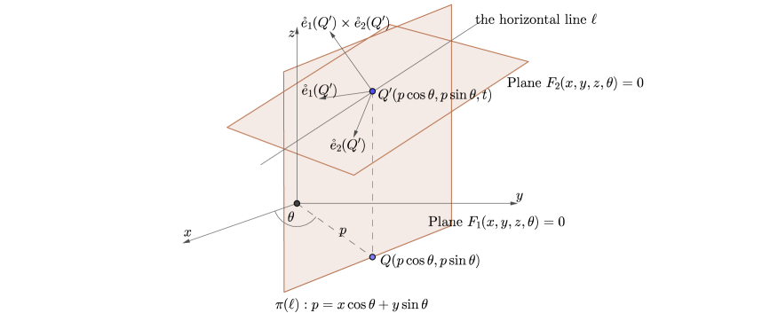
Fig. 1: Alternative expression of horizontal line $\ell$ in $\mathbb{H}_{1}$

By taking the derivatives, respectively, of $F_{1}$ and $F_{2}$ with respect to $\theta$, we have

$$\frac{\partial F_{1}}{\partial\theta} =-x\sin\theta+y\cos\theta-p^{\prime}=0,$$ (20)

$$\frac{\partial F_{2}}{\partial\theta} =(-p^{\prime}\sin\theta-p\cos\theta)x+(p^{\prime}\cos\theta-p\sin\theta)y-t^{\prime}=0.$$ (21)

Using (18), (20), and substituting $p$, $p^{\prime}$, into (21), the condition $\frac{\partial F_{2}}{\partial\theta}=0$ is equivalent to (12). Therefore, it may be only for seldom special cases that one can eliminate the parameter $\theta$ in (18), (19), and (20), to find the exact expression for the horizontal envelope.

2 Proofs of Theorems and Corollaries

In this section we shall give the proofs of Theorem 1 and 2. First we prove Proposition 1 which plays the essential role in the notes.

Proof.

(Proposition 1) Although the proof has been shown in [1] Proposition 8.2, for the self-contained reason we describe the proof here. Suppose $\pi(\ell)$ is the projection of horizontal line $\ell\in\mathbb{H}_{1}$ onto the $xy$-plane and the function $p=p(\theta)$ is the distance from the origin to $\pi(\ell)$ with angle $\theta$ from the positive direction of the $x$-axis (see Fig. 2).

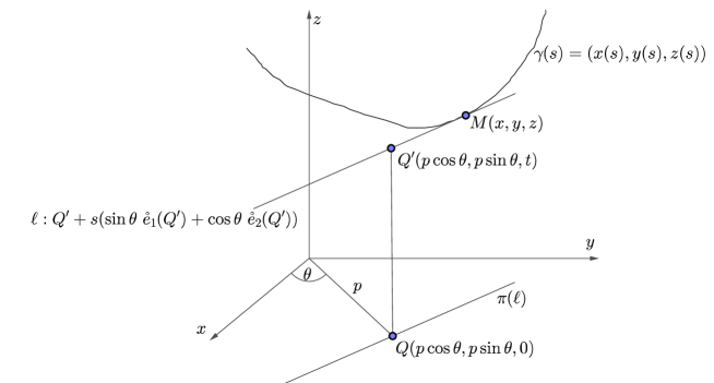
Fig. 2: The horizontal line $\ell$ in $\mathbb{H}_{1}$

Let the point $Q(p\cos\theta,p\sin\theta,0)$ be the intersection of the line through the origin perpendicular to $\pi(\ell)$. We choose the unit directional vector $(-\sin\theta,\cos\theta,0)$ along $\pi(\ell)$, and so any point $(x,y,0)$ on $\pi(\ell)$ can be parametrized by arc-length $s$

$$\left\{\begin{array}[]{rl}x&=p\cos\theta-s\ \sin\theta,\\ y&=p\sin\theta+s\ \cos\theta.\end{array}\right.$$ (24)

Denote the lift of the point $Q$ on $\ell$ by $Q^{\prime}$. We may assume $Q^{\prime}=(p\cos\theta,p\sin\theta,t)$ for some $t\in\mathbb{R}$. Since $\ell$ is horizontal, the tangent line of $\ell$ must be on the contact plane $\xi$. Thus, the parametric equations for $\ell$ can be represented by

$$\ell:(x,y,z)=(p\cos\theta,p\sin\theta,t)+s(A\mathring{e}_{1}(Q^{\prime})+B\mathring{e}_{2}(Q^{\prime})),$$ (25)

for some constants $A,B$ to be determined. Expand (25) by using the definitions of $\mathring{e}_{1}$ and $\mathring{e}_{2}$, and compare the coefficients with (24), one gets $A=-\sin\theta$ and $B=\cos\theta$. Thus, the parametric equations for $\ell$ are obtained as shown in (10). By (10), the parameters $p,\theta$, and $t$, uniquely determine the horizontal line $\ell$. ∎

Proposition 2.

Given any horizontal curve $\gamma(s)=(x(s),y(s),z(s))$ parametrized by horizontal arc-length $s$. Suppose the horizontal line $\ell$ determined by $(p,\theta,t)$ intersects $\gamma$ at the unique point $M(x,y,z)$ on the contact plane $\xi_{M}$ (see Fig. 2). If $p=p(\theta)$ is a function of $\theta$, then the intersection $M(x,y,z)$ can be uniquely represented by

$$\left\{\begin{array}[]{rl}x&=p\cos\theta-p^{\prime}\sin\theta,\\ y&=p\sin\theta+p^{\prime}\cos\theta,\\ z&=t-p^{\prime}p,\end{array}\right.$$ (29)

where $p^{\prime}$ denotes the partial derivative of the function $p$ with respect to $\theta$.

Proof.

We first solve the projection $(x,y,0)$ of the intersection $M$ onto the $xy$-plane in terms of $p$ and $\theta$, and then the $z$-component of $M$. By (24), any point $(x,y)$ on the projection of $\ell$ satisfies

$$p=x\cos\theta+y\sin\theta.$$ (30)

Since $p=p(\theta)$, take the derivative on both sides to get

$$p^{\prime}=-x\sin\theta+y\cos\theta.$$ (31)

Use (30) and (31) we obtain the first two components of the intersection $M$ on the $xy$-plane, namely,

$$x =p\cos\theta-p^{\prime}\sin\theta,$$

$$y =p\sin\theta+p^{\prime}\cos\theta.$$

To determine the third component of $M$, $z$, by using (24), (31), we have $s=y\cos\theta-x\sin\theta=p^{\prime}$. Finally, (10) implies that $z=t-p^{\prime}p$. The unique intersection point $M$ immediately implies the uniqueness of the expression (29) and the result follows. ∎

Now we prove Theorem 1.

Proof.

(Theorem 1) According to the assumptions for the functions $p$ and $t$, the curve $\gamma(\theta)=(x(\theta),y(\theta),z(\theta))$ defined by (16) is well-defined. By Proposition 4.1 [1], since any horizontally regular curve can be reparametrized by its horizontal arc-length, it suffices to show that the curve $\gamma(\theta)$ is horizontal. Indeed, by Proposition 2, a straight-forward calculation shows that

$$z^{\prime}-x^{\prime}y+y^{\prime}x$$

$$=\left(t^{\prime}-p^{\prime\prime}p-(p^{\prime})^{2}\right)-\left(p^{\prime}\cos\theta-p\sin\theta-p^{\prime\prime}\sin\theta-p^{\prime}\cos\theta\right)\left(p\sin\theta+p^{\prime}\cos\theta\right)$$

$$\hskip 28.45274pt+\left(p^{\prime}\sin\theta+p\cos\theta+p^{\prime\prime}\cos\theta-p^{\prime}\sin\theta\right)\left(p\cos\theta-p^{\prime}\sin\theta\right)$$

$$=t^{\prime}-(p^{\prime})^{2}+p^{2}.$$

Thus, $z^{\prime}-x^{\prime}y+y^{\prime}x=0$ if and only if the functions $p$ and $t$ satisfy (12). Therefore the curve defined by (16) is horizontal by (5).

To derive the p-curvature for the curve $\gamma$, substitute (16) into (6) and the result follows. It is also clear that $\tau\equiv 0$ since $\gamma$ is horizontal. ∎

The horizontal length of the horizontal envelope can be represented by the function $p(\theta)$. Actually, by (16) we have the horizontal length

$$L(\gamma):=\int_{0}^{2\pi}\left[\left(x^{\prime}(\theta)\right)^{2}+\left((y^{\prime}(\theta)\right)^{2}\right]^{1/2}d\theta=\int_{0}^{2\pi}|p+p^{\prime\prime}|d\theta.$$

Compare the p-curvature $k$ in Theorem 1 and the function on the right-hand side of the integral, we conclude that the length of the horizontal envelope $\gamma$ is the integral of the radius of curvature for the projection $\pi(\gamma)$

$$L(\gamma)=\int_{0}^{2\pi}\frac{1}{|k(\theta)|}d\theta.$$

Next we show Theorem 2.

Proof.

(Theorem 2) Suppose that the horizontal line $\ell$ represented by $(p,\theta,t)$ is tangent to $\gamma$ at $M(x,y,z)$. Since $M\in\ell$, by (10), we can solve the point $Q^{\prime}$ representing the horizontal line in terms of $x,y,z$. Let

$$x =p\cos\theta-s\ \sin\theta,$$ (32)

$$y =p\sin\theta+s\ \cos\theta,$$

$$z =t-sp.$$

One can solve

$$s=-x\sin\theta+y\cos\theta.$$ (33)

Substitute $s$ into the third equation in (32) to get

$$t=z+(-x\sin\theta+y\cos\theta)p$$ (34)

The first two equations in (32) imply that

$$p=x\cos\theta+y\sin\theta,$$ (35)

which means that the distance $p$ is a smooth function of $\theta$ defined on $[0,2\pi]$ if t$\ell$ intersects $\gamma$ at exactly one point. Similarly, (34) also implies that $t$ is a smooth function of $\theta$. Finally, use (33)(34)(35) it is easy to check that the horizontal line $\ell(p,\theta,t)$ satisfies the condition (12) for any $\theta$. ∎

Proof.

(Corollary 1) By Theorem 1, it suffices to show that the identity $t^{\prime}=(p^{\prime})^{2}-p^{2}$ holds. By assumption we have

$$t^{\prime}-(p^{\prime})^{2}+p^{2} =t_{1}^{\prime}+t_{2}^{\prime}-(p_{1}^{\prime}+p_{2}^{\prime})^{2}+(p_{1}+p_{2})^{2}$$

$$=-2p_{1}^{\prime}p_{2}^{\prime}+2p_{1}p_{2}.$$

Thus, $t^{\prime}=(p^{\prime})^{2}-p^{2}$ if and only if the identity $p_{1}^{\prime}p_{2}^{\prime}=p_{1}p_{2}$ holds. ∎

Proof.

(Corollary 2)

1. Take the derivatives for $p^{\prime}_{1}p^{\prime}_{2}=p_{1}p_{2}$ with respect to $\theta$, we have $p^{\prime\prime}_{1}p_{2}^{\prime}=p^{\prime}_{1}p_{2}+p_{1}p^{\prime}_{2}-p^{\prime}_{1}p^{\prime\prime}_{2}$. Use the assumptions for the signs of $p_{i}$, $p^{\prime}_{i}$, and $p^{\prime\prime}_{2}$, the left-hand side of the equation must be positive, and so $p^{\prime\prime}_{1}>0$.

2. The condition $p^{\prime}_{1}p^{\prime}_{2}=p_{1}p_{2}$ is equivalent to $p_{1}(\theta)=p_{1}(a)\exp{\int_{a}^{\theta}\frac{p_{2}}{p^{\prime}_{2}}d\alpha}$. Take the derivative twice we have $p^{\prime\prime}_{1}(\theta)=p_{1}(a)\exp{\int_{a}^{\theta}\frac{p_{2}}{p^{\prime}_{2}}d\alpha}\left(\frac{(p^{\prime}_{2})^{2}-p_{2}p^{\prime\prime}_{2}+(p_{2})^{2}}{(p^{\prime}_{2})^{2}}\right)$. Thus, the sign of $p^{\prime\prime}_{1}$ is only determined by the numerator

   $$(p^{\prime}_{2})^{2}-p_{2}p^{\prime\prime}_{2}+(p_{2})^{2}.$$ (36)

   We claim that $(p^{\prime}_{2})^{2}-p_{2}p^{\prime\prime}_{2}>0$ under the assumptions, and so (36) is positive. Indeed, if $p_{2},p^{\prime}_{2}>0$, then $0<\left(\log\frac{p_{2}}{p^{\prime}_{2}}\right)^{\prime}=\left(\log p_{2}\right)^{\prime}-\left(\log p^{\prime}_{2}\right)^{\prime}=\frac{p^{\prime}_{2}}{p_{2}}-\frac{p^{\prime\prime}_{2}}{p^{\prime}_{2}}$, and the result follows.

3. Use the similar method as (1).

4. Similar to (2), it suffices to show that the sign of (36) is negative. We shall show that $(p^{\prime}_{2})^{2}-\frac{p_{2}p^{\prime\prime}_{2}}{2}<0$ and $-\frac{p_{2}p^{\prime\prime}_{2}}{2}+(p_{2})^{2}<0$, and combine both inequalities to have the result. On one hand, since $p_{2}>0$ and $p^{\prime}_{2}<0$, we have $0<\left(\log\frac{p_{2}}{\sqrt{-p^{\prime}_{2}}}\right)^{\prime}=\left(\log p_{2}-\frac{1}{2}\log(-p^{\prime}_{2})\right)^{\prime}=\frac{p^{\prime}_{2}}{p_{2}}-\frac{p^{\prime\prime}_{2}}{2p^{\prime}_{2}}$, namely, $(p^{\prime}_{2})^{2}<\frac{p_{2}p^{\prime\prime}_{2}}{2}$. On the other hand, since $p^{\prime}_{2}<0$ and $-\frac{p^{\prime}_{2}}{p_{2}}=\left(\log\frac{1}{p_{2}}\right)^{\prime}>0>\frac{-2}{\left(\log(-p^{\prime}_{2})\right)^{\prime}}=\frac{-2p^{\prime}_{2}}{p^{\prime\prime}_{2}}$, one has $\frac{-p^{\prime}_{2}}{p_{2}}>\frac{-2p^{\prime}_{2}}{p^{\prime\prime}_{2}}$. Thus, multiply by $\frac{1}{-p^{\prime}_{2}}$ on both sides to have $\frac{p^{\prime\prime}_{2}}{2}>p_{2}$ which implies $\frac{p^{\prime\prime}_{2}p_{2}}{2}>(p_{2})^{2}$ and we complete the proof.

∎

Finally we point out that the construction in Corollary 1 can not obtain a closed horizontal envelope $\gamma$. Indeed, take the derivative with respect to $\theta$ in (16) and use (12), we have

$$z^{\prime}=t^{\prime}-(p^{\prime})^{2}-pp^{\prime\prime}=-p^{2}-pp^{\prime\prime},$$

which is equivalent to

$$z(\theta)=-\int_{0}^{\theta}p^{2}(\alpha)+p(\alpha)p^{\prime\prime}(\alpha)d\alpha+z(0)\ \text{, for any }\theta\in[0,2\pi].$$ (37)

If the curve was closed, say $z(0)=z(2\pi)$ and $p(0)=p(2\pi)$, by using Integration by Parts in (37) one gets

$$\int_{0}^{2\pi}p^{2}(\alpha)-\left(p^{\prime}(\alpha)\right)^{2}d\alpha=0.$$ (38)

However, according to Santaló [10] (equation (1.8) in I.1.2) we know that

$$F=\frac{1}{2}\int_{0}^{2\pi}p^{2}(\alpha)-(p^{\prime}(\alpha))^{2}d\alpha,$$

where $F$ is the enclosed area of the projection $\pi(\gamma)$ of the curve $\gamma$ on the $xy$-plane. Therefore, (38) is equivalent to that $\gamma$ must be a vertical line segment which contradicts with closeness of the curve.

References

• [1] Chiu H.-L, Huang Y.-C, Lai S.-H., An Application of the Moving Frame Method to Integral Geometry in the Heisenberg Group Symmetry, Integrability and Geometry: Methods and Applications, 13 (2017), 097, arXiv:1509.00950v3.
• [2] Clausen A., Strub C., A General and Intuitive Envelope Theorem, Edinburgh School of Economics Discussion Paper Series, ESE Discussion Papers; No. 274.
• [3] Eisenhart L.P., A Treatise on the Differential Geometry of Curves and Surfaces, 1909, HardPress Publishing, ISBN-1314605879 (reprint 2013).
• [4] Griebelery M.C., AraΓΊjo J.P., General envelope theorems for multidimensional type spaces, The 31nd Meeting of the Brazilian Econometric Society, 2009.
• [5] Gromov M., Carnot-CarathΓ©odory spaces seen from within, Sub-riemannian geometry, Prog. Math., vol 144, Birkh’́auser, Basel, 1996, 79-323.
• [6] Marenich V., Geodesics in Heisenberg Groups, Geometriae Dedicata, 1997, Volume 66, Issue 2, pp 175-185.
• [7] Milgrom P., Sega I., Envelope theorems for arbitrary choice sets, Econometrica, Volume 70, Issue 2, 2002, pp 583-601.
• [8] Monti R., Rickly M., Geodetically Convex Sets in the Heisenberg Group, Journal of Convex Analysis, Volume 12, (2005), No. 1, 187-196.
• [9] RitorΓ© M., Rosales C., Area-stationary surfaces in the Heisenberg group $H^{1}$, Advances in Mathematics, v219, Issue 2, 2008, 633-671.
• [10] SantalΓ³ L.A., Integral geometry and geometric probability, 2nd ed., Cambridge Mathematical Library, Cambridge University Press, Cambridge, 2004.