SDSS IV MaNGA: Dependence of Global and Spatially-resolved SFR-M_∗ Relations on Galaxy Properties

Abstract

Galaxy integrated H$\alpha$ star formation rate-stellar mass relation, or SFR(global)-M_∗(global) relation, is crucial for understanding star formation history and evolution of galaxies. However, many studies have dealt with SFR using unresolved measurements, which makes it difficult to separate out the contamination from other ionizing sources, such as active galactic nuclei (AGN) and evolved stars. Using the integral field spectroscopic observations from SDSS-IV MaNGA, we spatially disentangle the contribution from different H$\alpha$ powering sources for $\sim$1000 galaxies. We find that, when including regions dominated by all ionizing sources in galaxies, the spatially-resolved relation between H$\alpha$ surface density ($\Sigma_{\mathrm{H\alpha}}$(all)) and stellar mass surface density ($\Sigma_{\ast}$(all)) progressively turns over at high $\Sigma_{\ast}$(all) end for increasing M_∗(global) and/or bulge dominance (bulge-to-total light ratio, B/T). This in turn leads to the flattening of the integrated H$\alpha$(global)-M_∗(global) relation in the literature. By contrast, there is no noticeable flattening in both integrated H$\alpha$(HII)-M_∗(HII) and spatially-resolved $\Sigma_{\mathrm{H\alpha}}$(HII)-$\Sigma_{\ast}$(HII) relations when only regions where star formation dominates the ionization are considered. In other words, the flattening can be attributed to the increasing regions powered by non-star-formation sources, which generally have lower ionizing ability than star formation. Analysis of the fractional contribution of non-star-formation sources to total H$\alpha$ luminosity of a galaxy suggests a decreasing role of star formation as an ionizing source toward high-mass, high-B/T galaxies and bulge regions. This result indicates that the appearance of the galaxy integrated SFR-M_∗ relation critically depends on their global properties (M_∗(global) and B/T) and relative abundances of various ionizing sources within the galaxies.

1 Introduction

The relation between galaxy star formation rate (SFR) and stellar mass (M_∗) provides key constraints on the star formation history and mass assembly of galaxies. Star-forming galaxies, populated by disk-dominated galaxies, form a tight relationship on the SFR-M_∗ plane, the so-called “star-forming main sequence”, which can be described by a power-law relation (Noeske et al., 2007; Elbaz et al., 2011; Catalán-Torrecilla et al., 2015; Lee et al., 2015). On the other hand, the quiescent population, primarily composed of bulge-dominated galaxies (e.g., Wuyts et al., 2011), has a much lower specific star formation rate (sSFR $\equiv$ SFR/M_∗) with respect to the main sequence. Several studies have suggested that the main sequence relation flattens at high mass end, possibly due to the growth of the bulge that lower the global sSFR of a galaxy (Noeske et al., 2007; Abramson et al., 2014; Whitaker et al., 2015; Catalán-Torrecilla et al., 2017).

Although the SFR-M_∗ relation has been reported with a variety of different data sets, their appearance can vary significantly from one to another. A key uncertainty occurs in the SFR measurement. H$\alpha$ is frequently utilized as SFR indicators. However, it has long been known that young star is not the only powering source of H$\alpha$. Other sources such as active galactic nucleus (AGN) and old stellar population also contribute to H$\alpha$ (Yan & Blanton, 2012; Singh et al., 2013; Belfiore et al., 2016) and therefore affect the SFR-M_∗ relation.

Since star formation is an intrinsically local process, further insight into the nature of SFR-M_∗ relation would require spatially-resolved data to understand what processes drive the connection between SFR and M_∗. Using spatially-resolved spectroscopy, recent studies have shown that there also exist a tight correlation between SFR and stellar mass surface density for nearby and distant star-forming galaxies (Nelson et al., 2012; Wuyts et al., 2013; Cano-Díaz et al., 2016; Abdurro’uf & Akiyama, 2017; Hsieh et al., 2017; Ellison et al., 2017). Recently, Hsieh et al. (2017) extends the study to the quiescent population using the MaNGA survey (Mapping Nearby Galaxies at APO; Bundy et al., 2015) and find that the emission line fluxes, even classified as LI(N)ER, are also correlated with the underlying stellar mass surface density. Therefore, it is essential to separate out the contribution of non-star-forming regions when measuring the SFR based on emission line methods. This also has an important application to galaxy formation models as the SFR-M_∗ relation is often used to validate the subgrid physics modeling (Tissera et al., 2016; Lagos et al., 2016).

The main aim of this paper is to show that the galaxy SFR-M_∗ relation is sensitive to whether or not the “contamination” is removed. Since H$\alpha$ does not only trace star formation, throughout the paper we refer to SFR-M_∗ relation as H$\alpha$-M_∗ relation. SFR axis and sSFR lines are provided for readers to compare with other studies.

We present our study as follows: in Section 2, we describe our sample and data, and present the traditional global H$\alpha$-M_∗ relation making use of the total H$\alpha$ luminosity and M_∗ of galaxies. Section 3 compares the spatially-resolved H$\alpha$-M_∗ surface density relation before and after the non-star-formation sources being removed. Section 4 quantifies the contribution of the non-star-formation source as a function of galaxy properties and compares the integrated H$\alpha$-M_∗ relations with and without the non-star-formation contributions being removed. Main results are summarized in Section 5.

2 Data and the Traditional Global H$\alpha$-M_∗ Relation

2.1 MaNGA Survey

The advent of MaNGA survey (Bundy et al., 2015; Law et al., 2015; Yan et al., 2016a), which spatially resolves stellar and gas properties, offers an excellent opportunity to examine the H$\alpha$-M_∗ relation. MaNGA is part of the fourth generation of the Sloan Digital Sky Survey (SDSS-IV; Gunn et al., 2006; Blanton et al., 2017) and aims to obtain spatially-resolved spectroscopy of 10,000 galaxies with median redshift $\sim$ 0.03 by 2020. Further details on the MaNGA sample selection can be found in Wake et al. (2017). MaNGA has a wavelength coverage of 3600 – 10300 Å, with a spectral resolution varying from $R$ $\sim$ 1400 at 4000 Å  to $R$ $\sim$ 2600 around 9000 Å (Smee et al., 2013; Yan et al., 2016b). MaNGA uses 5 different types of IFU, ranging in diameter from 19 (12.5$\arcsec$) to 127 fibers (32.5$\arcsec$). The IFUs are installed in six SDSS cartridges. Each MaNGA cartridge has 17 science IFUs and 12 seven-fiber IFUs for calibration. The IFU sizes and the number density of galaxies on the sky were designed jointly to allow more efficient use of IFUs (e.g., minimize the number of IFUs that are unused due to tile with too few galaxies), and to allow to observe galaxies in the redshift range to at least 1.5 effective radii (Drory et al., 2015; Wake et al., 2017).

This study draws data from the fourth MaNGA Product Launches (MPL-4), corresponding to SDSS DR13 (Albereti et al., 2017). The observational data was reduced using the MaNGA data-reduction-pipeline (DRP; Law et al., 2016).

2.2 Local and Global SFR and M_∗ Measurements

The reduced spaxel-wise data cubes were analyzed using the Pipe3D pipeline to extract the physical parameters from each of the spaxels in each galaxy. Pipe3D fits the continuum with stellar population models and measures the nebular emission lines. Details of the procedures and uncertainties of the process are described in Sánchez et al. (2016a, b) and Sanchez et al. (2017).

We briefly summarize the fitting of stellar continuum and the derivation of emission line flux here. The stellar continuum was first modeled using a simple-stellar-population (SSP) library with 156 SSPs, comprising 39 ages and 4 metallicities (Cid Fernandes et al., 2013; Sánchez et al., 2016b). Before the fitting, spatial binning is performed to reach a signal-to-noise ratio (S/N) of 50 across the field of view. Then the stellar population fitting was applied to the coadded spectra within each spatial bin. Finally, the stellar population model for spaxels with continuum S/N $>$ 3 is derived by re-scaling the best fitted model within each spatial bin to the continuum flux intensity in the corresponding spaxel. The stellar mass is obtained using the stellar populations derived for each spaxel, then normalized to the physical area of one spaxel to get the surface density ($\Sigma_{\ast}$) in unit of M_☉ kpc^-2. The stellar mass per spaxel is also coadded to derive the integrated stellar mass of the galaxies (M_∗(global)).

The stellar-population model are subtracted from the data cube to create an ionized gas emission line cube (with noise). The emission line fluxes were measured spaxel by spaxel. The SFR was derived using the H$\alpha$ emission line. It is again possible to compute the total H$\alpha$ luminosity (H$\alpha$(global)) and SFR (SFR(global)) by integrating the spatially-resolved quantities over spaxels. The integrated H$\alpha$ luminosity were derived using the H$\alpha$ fluxes for all the spaxels with S/N $>$ 3.

To study the effect of non-star formation powered H$\alpha$ on the H$\alpha$-M_∗ relation, we use a set of emission line ratios to spatially distinguish the ionization mechanisms of H$\alpha$ in galaxies (see §3.2). To ensure reliable emission line ratios, we also limit the spatially-resolved analysis to spaxels with S/N(H$\alpha$), S/N(H$\beta$), S/N([O III]), and S/N([N II]) $>$ 3. The fluxes are converted to luminosities and corrected for extinction. The method described in the Appendix of Vogt et al. (2013) is used to compute the reddening using the Balmer decrement at each spaxel of the IFU cube. The extinction-corrected H$\alpha$ luminosity is converted into SFR surface density ($\Sigma_{\mathrm{SFR}}$ in M_☉ yr^-1 kpc^-2) using the empirical calibration from Kennicutt (1998) that adopts the Salpeter IMF.

Inclination correction is applied to the H$\alpha$ luminosity and stellar mass of all spaxels of a galaxy equally. Galaxy inclination measured by the disk ellipticity in Simard et al. (2011) is adopted (see the next section). Such correction is based on the assumption of thin disks, whereas for round bulges or more spheroidal galaxies it may systematically overestimate the effect of projection and thus underestimate the H$\alpha$ luminosity and stellar mass. However, we also note that the correction does not affect the sSFR related quantities since it is applied to both H$\alpha$ luminosity and stellar mass.

MaNGA galaxies are selected to have spectroscopic coverage to 1.5 – 2.5 effective radii ($R_{e}$). The exact range varies from galaxy to galaxy. The mean offset between the Pipe3D M_∗(global) and the aperture-corrected NSA stellar mass is 0.07 dex, corresponding to the difference between the adopted cosmologies and the differences in IMFs. We then assume that the aperture effect has minimal impact on the stellar mass. To estimate how much of the SFR in a galaxy may be unaccounted for due to the finite fiber aperture, we assume that H$\alpha$ following a simple exponential profile out to infinite radius. The disk exponential profile in $r$-band of each galaxy derived by Simard et al. (2011) is adopted. We estimate the total SFR out to infinite radii and SFR inside the MaNGA IFUs for all galaxies, and find that most of the star formation (on average, 84 $\pm$ 15%) occurs within the MaNGA IFUs. In light of this, we assume that the aperture effect does not significantly affect the SFR measurement as well.

MaNGA targets galaxies in the redshift range 0.01 $<$ $z$ $<$ 0.15 (Wake et al., 2017). Since the spatial resolution is different across the sample, we repeat the analysis in this work by using the sub-samples selected by distance. The main results are not severely affected by the varying physical size of spaxels.

2.3 The Bulge-Disk Decomposition

Galaxy structural parameters are taken from the bulge-disk decomposition catalog from Simard et al. (2011). Simard et al. (2011) perform the two-dimensional bulge and disk decompositions using the GIM2D software package (Simard et al., 2002) on the g-band and r-band images of SDSS DR7 galaxies. In the model, the bulge Sérsic index ($n$) is treated as a free parameter and the disk component has $n$ $=$ 1. Structural parameters measured in r-band are used in this work. We use the bulge-to-total light ratio (B/T) as a proxy for bugle dominance. The bulge and disk regions are separated by the radius at which 50% of the light is contributed by the bulge and disk component respectively. Specifically, for each galaxy, we look for the intersection of the one-dimensional fractional r-band Sérsic profile of bulge and the exponential profile of disk. It must be noted that the radius does not indicate the physical size of the bulge, but the boundary of the bulge-dominated and the disk-dominated regions.

The sample has been selected to only include galaxies that have measurements from both Pipe3D and Simard et al. (2011). With this requirement, 1037 out of $\sim$1400 galaxies in MPL-4 are left.

2.4 Traditional Global H$\alpha$-M_∗ Relation

Figure 1 shows the H$\alpha$(global)-M_∗(global) relation using total H$\alpha$ luminosity and M_∗ of galaxies. The small circles present the individual galaxies color-coded by B/T from white to black. The dashed lines denote log(sSFR/yr^-1) of -9.5, -10.5, and -11.5 (from top to bottom). As reported in the literature, galaxies populate two distinct sequences, with a clear separation between star-forming and quiescent galaxies.

To characterize the dependence of the H$\alpha$(global)-M_∗(global) relation on B/T and M_∗(global), we binned the galaxies by these two quantities. Big circles are the median values of H$\alpha$(global) of the whole sample in different M_∗(global) bins, colored according to B/T (following the scheme of Fig. 2 in Whitaker et al. (2015)). The discontinuity in the median values of H$\alpha$(global) at log(M_∗(global)/M_⊙) $\sim$ 10 is caused by decreasing number of quiescent targets in the low mass end.

As been noticed by many authors (e.g., Wuyts et al., 2011), the sequence with lower H$\alpha$(global)-to-M_∗(global) ratio, i.e., lower sSFR(global), is occupied prevalently by bulge-dominated galaxies (B/T $\geq$ 0.2), whereas the star-forming sequence is composed of all populations (but note that disk-dominated galaxies with B/T $<$ 0.2 appear to be almost exclusively star-forming galaxies). A flattening of the lower-B/T galaxies ($\sim$ 0.2) at log(M_∗(global)/M_⊙) $>$ 11 is observed. This has been explained as the increasing fraction of the mass being given by bulges that have begun to quench, indicating a transition from disk to bulge-dominated properties.

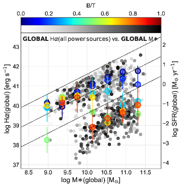
Figure 1: Integrated H$\alpha$(global)-M_∗(global) relation for individual galaxies (small circles) derived from the Pipe3D analysis, color-coded by their B/T from white to black. Colored circles are the median values of log(H$\alpha$(global)/erg s^-1) of the whole sample in different M_∗ and B/T bins, color-coded by B/T (following the scheme of Fig. 2 in Whitaker et al. (2015)). The error bars are given by the standard deviation in each bin. The dashed lines represent log(sSFR/yr^-1) of -9.5, -10.5, and -11.5 (from top to bottom).

3 Spatially-Resolved H$\alpha$-M_∗ Relation

3.1 Spatially-Resolved H$\alpha$-M_∗ Relation Using All Spaxels in Galaxies

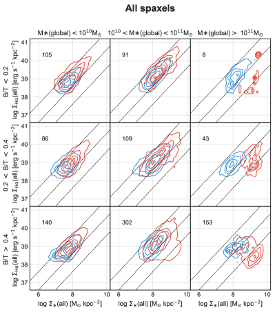
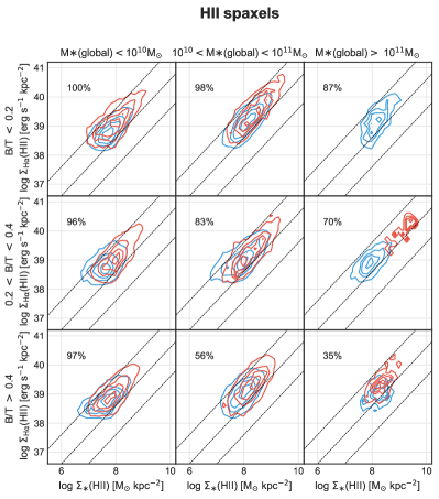
Figure 2: (a) Inclination-corrected spatially-resolved $\Sigma_{\mathrm{H\alpha}}$(all)-$\Sigma_{\ast}$(all) relation. All spaxels (S/N $>$ 3) powered by all ionizing mechanisms in the galaxies are used to make the plot. Blue and red contours denote the spaxels from disk and bulge, respectively. B/T and M$\ast$(global) increase from the top to bottom and the left to right. In other words, from upper-left to bottom-right sub-panel, galaxies go from disk-dominated to bulge-dominated. Number of galaxy in each bins is indicated at the upper-left corner of the sub-panels. The contours represent 15, 40, 60, and 85% of the peak counts, per 0.15 dex-wide cell. The dashed lines denote log(sSFR/yr^-1) of -9.5, -10.5, and -11.5 (from top to bottom). (b) Inclination-corrected $\Sigma_{\mathrm{H\alpha}}$(HII)-$\Sigma_{\ast}$(HII) relation. Only HII spaxels (i.e. star-forming regions) are used. The percentage value in the upper-left corner of each sub-panel indicates the number fraction of galaxies with HII spaxels relative to the number of galaxies in each bin in panel (a).

The spatially-resolved $\Sigma_{\mathrm{H\alpha}}$ and $\Sigma_{\ast}$ maps of MaNGA allow us to probe the driver of the H$\alpha$(global)-M_∗(global) relation in more detail. Figure 2 presents the inclination-corrected spatially-resolved $\Sigma_{\mathrm{H\alpha}}$(all)-$\Sigma_{\ast}$(all) relation using all spaxels of galaxies. The galaxies are binned by their M_∗(global) and B/T: from the upper-left to the bottom-right sub-panel, galaxies go from disk-dominated to bulge-dominated. Number of galaxy in each bins is indicated in the upper-left corner. Bulge and disk regions are shown by red and blue contours, respectively. Number of spaxel in each sub-panel ranges from $\sim$ 900 to 39000 for the bulge and $\sim$ 6500 to 70000 for the disk.

For galaxies with log(M_∗(global)/M_⊙) $<$ 10, bulge and disk lie along a similar $\Sigma_{\mathrm{H\alpha}}$(all)-$\Sigma_{\ast}$(all) relation. As the stellar mass increases to 10 $<$ log(M_∗(global)/M_⊙) $<$ 11, the high-mass ends of bulge sequence start to move downward (i.e., decrease in the $\Sigma_{\mathrm{H\alpha}}$(all)-to-$\Sigma_{\ast}$(all) ratio). The decrease is more pronounced in the high-B/T galaxies than in the low-B/T galaxies. In the most massive galaxies (log(M_∗(global)/M_⊙) $>$ 11), the entire bulge sequence drops below the relations of the lower-mass objects. Meanwhile, the disk sequence also shows a slight drop in the $\Sigma_{\mathrm{H\alpha}}$(all)-to-$\Sigma_{\ast}$(all) ratio at the log(M_∗(global)/M_⊙) and B/T values above 10 and 0.4, respectively (lower-right sub-panel). The combination of these leads to the high-M_∗(global) and/or high-B/T systems being pulled off the main sequence on the integrated H$\alpha$(global)-M_∗(global) plane. Such turnover also indicates the inside-out quenching of galaxies. The quenching process is beyond the scope of the present paper, but is of major importance in the context of galaxy evolution (e.g., Li et al., 2015; González Delgado et al., 2016; Belfiore et al., 2017; Lin et al., 2017; Ellison et al., 2017; Spindler et al., 2017).

3.2 Spatially-Resolved H$\alpha$-M_∗ Relation Using Star-Formation Spaxels in Galaxies

We now turn our attention to the powering source of H$\alpha$. It is known that massive stars are not the only source capable of providing ionizing photons. To disentangle different powering sources, we use the emission line ratio diagnostics, the BPT diagram (Baldwin et al., 1981) and H$\alpha$ equivalent width (EW) to spatially identify the regions ionized by different physical processes in each galaxy. The emission line regions are classified into star-forming HII regions, LI(N)ER, Seyfert, and composite regions (mix of multiple sources) based on their locations on the [O III] 5007/H$\beta$ versus [N II] 6584/H$\alpha$ plane (Kewley et al., 2001; Kauffmann et al., 2003; Cid Fernandes et al., 2010). In addition, the criterion of EW $>$ 6Å  is also applied when selecting star-forming regions (Sánchez et al., 2014; Sanchez et al., 2017).

Armed with the spatially-resolved ionization sources of each galaxy, we use the identified HII spaxels to construct the $\Sigma_{\mathrm{H\alpha}}$(HII)-$\Sigma_{\ast}$(HII) relation driven by star formation alone. The result is presented in Figure 2. For the star-forming regions, $\Sigma_{\mathrm{H\alpha}}$(HII) and $\Sigma_{\ast}$(HII) is much more tightly correlated than that including all ionized regions of the galaxies. Moreover, the bulge sequence shifts upwards to be close to that of disk. In other words, at least for the star-forming regions, the $\Sigma_{\mathrm{H\alpha}}$(HII)-to-$\Sigma_{\ast}$(HII) ratio of bulge and disk, which is proportional to the local sSFR, do not differ significantly from each other. In light of this, the turnover seen in the $\Sigma_{\mathrm{H\alpha}}$(all)-$\Sigma_{\ast}$(all) relation can be attributed to non-HII regions; moreover, the non-HII ionizing sources tend to generate lower H$\alpha$ luminosity than that of star-forming regions and the difference can vary by up to an order of magnitude. Therefore, the total H$\alpha$ luminosity of a galaxy strongly depends on the relative proportion between HII and non-HII regions.

Another notable feature in Figure 2 is the lack of HII spaxles towards higher masses and higher B/T. The number fraction of galaxies with HII spaxels relative to the total number of galaxies in each bin is given in the upper-left corner of each sub-panel. The fraction is generally inversely correlated with M_∗(global) and B/T, suggesting a decreasing role of star formation as an ionizing source towards high-mass and high-B/T galaxies.

4 Revisit the Integrated Relations

The previous section indicates that the flattening of the spatially-resolved bulge sequence can be attributed to the non-HII sources, which generally have lower ionizing ability compared to young stars, and such contribution become more significant with increasing M_∗(global) and B/T. It is therefore worth quantifying the contribution of non-HII powering sources in different galaxy populations and sub-galactic structures, and revisiting the integrated H$\alpha$-M_∗ relation of galaxies.

4.1 Quantitative Contribution of Non-HII Powering Sources

The box plots in Figure 3 describe the distribution of the fraction of non-HII contribution in the total H$\alpha$ luminosity of a galaxy ($f_{\mathrm{nonHII}}$) in different M_∗(global) bins. Three columns from left respectively present the fraction of H$\alpha$ contributed by composite, LI(N)ER, and Seyfert, respectively, e.g., in the left-most column, $f_{\mathrm{nonHII}}$ $=$ H$\alpha$(composite)/H$\alpha$(global). The green line drawn across the box is the sample median. The ends of the box are the upper and lower quartiles (the interquartile range, IQR), i.e., 50% of the sample is located in the box. The two whiskers (vertical lines) outside the box extend to 1.5 $\times$ IQR, i.e., 99% of the sample is inside the caps of the whiskers. In the following paragraphs, we will discuss $f_{\mathrm{nonHII}}$ as a function of M_∗(global), B/T, and galactic sub-structures.

Figure 3 presents the dependence of $f_{\mathrm{nonHII}}$ on the bulge dominance, B/T. The upper and lower rows show the results for B/T $<$ 0.2 and $>$ 0.2, respectively. Several features are readily apparent. Most notably, the (non-zero) median $f_{\mathrm{nonHII}}$ increases in general with increasing M_∗(global) in both populations, suggesting that the non-HII sources become more important with increasing M_∗(global) (see also Catalán-Torrecilla et al., 2017). For some M_∗(global) bins, the median and the whiskers are subsumed in a single location due the large number of galaxies with small $f_{\mathrm{nonHII}}$.

Moreover, in the bulge-dominated galaxies, the non-HII contribution is exclusively dominated by LI(N)ER, whereas the three mechanisms all make a certain contribution, but typically lower than LI(N)ER in the high-B/T galaxies, in the disk-dominated galaxies. This originates from the fact that the old stellar population, such as post-AGBs stars, have become the main source of ionizing photons after star formation has ceased (Yan & Blanton, 2012; Singh et al., 2013; Belfiore et al., 2016; Hsieh et al., 2017). As a whole, the right-most column shows that $f_{\mathrm{nonHII}}$ increases from less than a percent for log(M_∗/M_⊙) $<$ 10 to a few to several tens percent at log(M_∗/M_⊙) $>$ 10. Besides, high-B/T galaxies generally display a higher, or just comparable, median $f_{\mathrm{nonHII}}$ to the low-B/T galaxies over the all range of masses.

Figure 3 explores the dependence of $f_{\mathrm{nonHII}}$ on sub-galactic regions. The upper and lower rows show the disk and bulge regions, respectively. Bulges generally exhibit higher fraction of non-HII contribution than the disks, and the non-zero median $f_{\mathrm{nonHII}}$ increases with increasing M_∗(global). When accounting for all non-HII mechanisms (the right-most column), median $f_{\mathrm{nonHII}}$ is no higher than 20% (mostly below 10%) for disks across all stellar mass bins, and increases to several tens percent in bulges when log(M_∗/M_⊙) exceeding 10. The result is consistent with the study based on a 2D spectral decomposition of the bulge and disk component (Catalán-Torrecilla et al., 2017). The high $f_{\mathrm{nonHII}}$ of bulge is presumably due to the fact that the non-HII sources (e.g., AGNs, evolved stars, and shocks) are naturally found most often in this old central component. The above-mentioned characteristics echo the turnover feature of bulge $\Sigma_{\mathrm{H\alpha}}$(all)-$\Sigma_{\ast}$(all) relation towards higher masses and higher B/T in Figure 2.

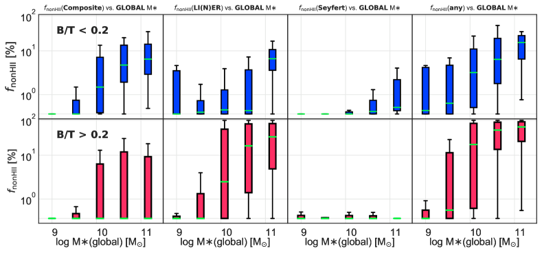
Figure 3: Box plots showing the $f_{\mathrm{nonHII}}$ distribution for each of the M_∗(global) bin. In each plot the median is indicated by the green bar in the middle. The ends of the box are the upper and lower quartiles (the interquartile range, IQR), 50% of the sample is located in the box. The two whiskers (vertical lines) outside the box extend to 1.5 $\times$ IQR, 99% of the sample is inside the caps of the whiskers. In some stellar mass bins, the median and the whiskers are subsumed in a single location due the large number of galaxies with small $f_{\mathrm{nonHII}}$. Panel (a) shows $f_{\mathrm{nonHII}}$ in each B/T for each M_∗(global). The upper row shows the results for galaxies with B/T $<$ 0.2 (disk-dominated galaxies), the lower row shows galaxies with B/T $>$ 0.2 (bulge-dominated galaxies). From left to right, the sub-panels present the $f_{\mathrm{nonHII}}$ of composite, LI(N)ER, and Seyfert, respectively. Panel (b) shows the dependency of $f_{\mathrm{nonHII}}$ on galactic sub-regions, with disks in the upper row and bulges in the lower row).

4.2 Revisiting the Integrated H$\alpha$-M_∗ Relation

How does the integrated H$\alpha$-M_∗ relation look like after excluding the non-HII contribution? Figure 4 shows the integrated H$\alpha$(HII)-M_∗(HII) relation in panel (a), the H$\alpha$(HII)-M_∗(global) relation in panel (b), and the traditional H$\alpha$(global)-M_∗(global) relation in panel (c) (same as Figure 1), where H$\alpha$(HII) and M_∗(HII) represent H$\alpha$ and M_∗ integrated over only HII spaxels in galaxies. Symbol styles and colours are as in the Figure 1. We note here that, the H$\alpha$(HII) distribution could become highly skewed if there are extreme values, such as zero value. In this case, the standard deviation, which is shown as error bars here, would become meaningless. This affects only Figure 2, so the error bars are thus omitted in this plot.

Figure 4 represents the integrated relation for star-forming regions. When only looking at star-forming regions, the H$\alpha$(HII)-M_∗(HII) relation shows a relatively tight sequence. The figure is simply an integrated version of Figure 2. As noted before, the spatially-resolved relations become similar for the bulge and disk when accounting for only star-forming regions. This leads naturally to the tight and close to linear correlation in the integrated H$\alpha$(HII)-M_∗(HII) relation.

We now shift our focus to the H$\alpha$(HII)-M_∗(global) relation in Figure 4. For reference, the traditional H$\alpha$(global)-M_∗(global) relation is displayed in Figure 4. The most noticeable feature in Figure 4 is the emergence of galaxies with low H$\alpha$(HII)-to-M_∗(global) ratio (lower than the H$\alpha$(global)-to-M_∗(global) ratio of quiescent galaxies in the traditional relation). This population is largely comprised of the quiescent galaxies, which are dominated by non-HII regions. Note that since significant fraction of the highest-B/T and highest-mass galaxies have little to no H$\alpha$ from star formation, the median H$\alpha$(HII) of these populations drop to close to zero.

It is worth noting also that the strong sequence of quiescent galaxies observed in the traditional relation becomes scattered in the H$\alpha$(HII)-M_∗(global) relation; no clear scaling relation is found between H$\alpha$(HII) and M_∗(global) for this population. Such a lack of bimodality in the SFR distribution at a given stellar mass is very similar to that using the SSP-based SFR by González Delgado et al. (2016) and using MAGPHYS rather than based on H$\alpha$ by Eales et al. (2017).

Then what processes fundamentally drive the two strong sequences in the traditional H$\alpha$(global)-M_∗(global) relation in Figure 1? From left to right, the four panels in Figure 5 respectively present the H$\alpha$ luminosity integrated over star formation spaxels (same as Figure 4), composite spaxels, LI(N)ER spaxels, and Seyfert spaxels against M_∗(global). The high H$\alpha$-to-M_∗ ratio regime is heavily populated by star formation, while other mechanisms occupy the low ratio regime. The H$\alpha$(composite)-M_∗(global) and H$\alpha$(Seyfert)-M_∗(global) relations show relatively large scatter for a given M_∗(global), on the other hand, H$\alpha$(LI(N)ER) and M_∗(global) appear to be more tightly correlated to each other. The relation is very similar to the quiescent population in the traditional H$\alpha$(global)-M_∗(global) relation. In other words, H$\alpha$ powered by LI(N)ER is directly correlated with the underlying stellar mass. This has been explained as the hot, evolved stars as the dominant mechanism powering the H$\alpha$ emission in quiescent galaxies (e.g., Belfiore et al., 2016; Hsieh et al., 2017). Our Figure 3 is also in line with this scenario.

Finally, we remind the reader that the non-HII spaxels are not necessarily devoid of star formation, but simply being dominated by mechanisms other than star formation. That is to say, the H$\alpha$(global)-M_∗(global) relation and the H$\alpha$(HII)-M_∗(global) relation represent bracketing scenarios as the true SFR of the galaxies would be found between H$\alpha$(HII) and H$\alpha$(global). Moreover, the flatting (or turnover) of the integrated SFR-M_∗ relation would become more pronounced as we move from the traditional integrated SFR(global)-M_∗(global) relation to the true SFR versus M_∗(global) relation.

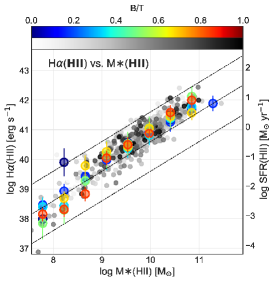
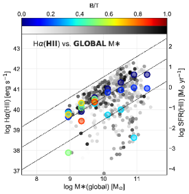
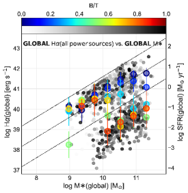
Figure 4: Integrated H$\alpha$ and M_∗ relations. Individual objects are shown by small circles. Colored circles are the median values of log(H$\alpha$) of the whole sample in different M_∗ and B/T bins. The error bars are given by the standard deviation in each bin. The dashed lines represent log(sSFR/yr^-1) of -9.5, -10.5, and -11.5 (from top to bottom). (a) Integrated H$\alpha$(HII)-M_∗(HII) relation, where H$\alpha$(HII) and M_∗(HII) represent the H$\alpha$ luminosity and stellar mass integrated over only HII spaxels in galaxies. In other words, the figure represents the integrated relation for star-forming regions. (b) Integrated H$\alpha$(HII) versus M_∗(global) relation. Since the zero-H$\alpha$(HII) are taken into account when computing the median H$\alpha$(HII) (color circles), the standard deviation become meaningless due to the highly skewed H$\alpha$(HII) distribution. The error bars are thus omitted in this plot. (c) Traditional integrated H$\alpha$(global)-M_∗(global) relation, same as Figure 1.

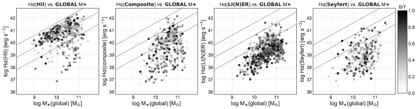
Figure 5: Integrated H$\alpha$(HII), H$\alpha$(composite), H$\alpha$(LI(N)ER), and H$\alpha$(Seyfert) against M_∗(global). From left to right, the $y$-axes are H$\alpha$ luminosity integrated over HII (same as Figure 4), composite, LI(N)ER, and Seyfert regions in galaxies, respectively. The circles represent individual galaxies, color-coded by B/T. For reader to compare the plots with other figures, the corresponding lines of log(sSFR/yr^-1) $=$ -9.5, -10.5, and -11.5 (from top to bottom) are shown in all panels.

5 Summary

In this work, we present the analysis of the global and spatially-resolved H$\alpha$-M_∗ relations using a sample of $\sim$ 1000 galaxies from the MaNGA survey (§2). By virtue of the spatially-resolved spectroscopic data from MaNGA, we spatially identified the regions ionized by different physical processes in each galaxy (§3). Our main conclusions are summarized below.

1. When all H$\alpha$ powering mechanisms are considered, the spatially-resolved $\Sigma_{\mathrm{H\alpha}}$(all)-$\Sigma_{\ast}$(all) relation of bulges progressively turns over to below the disk sequence for increasing values of M_∗(global) and/or B/T (Figure 2). At the same time, disk sequence is relatively insensitive to galaxy stellar mass and B/T. This in turn leads to the frequently reported flattening of the integrated H$\alpha$(global)-M_∗(global) relation in the literature (Figure 1).

2. On the other hand, we find little evidence for the flattening of both integrated H$\alpha$(HII)-M_∗(HII) and spatially-resolved $\Sigma_{\mathrm{H\alpha}}$(HII)-$\Sigma_{\ast}$(HII) relations when the star-forming regions alone are considered (Figure 2 and 4).

3. The fractional contribution of non-HII sources to total H$\alpha$ luminosity of a galaxy increases with increasing B/T and M_∗(global), and increases from disk to bulge regions, suggesting a decreasing role of star formation as an ionizing source toward high-mass, high-B/T galaxies and bulge regions (§4.1 and Figure 3). Moreover, the non-HII sources tend to have lower ionizing ability compared to star formation.

4. We discussed the difference between the traditional H$\alpha$(global)-M_∗(global) relation and H$\alpha$(HII)-M_∗(global) relation (§4.2 and Figure 4). There is no clear scaling relation between H$\alpha$(HII) and M_∗(global) for the quiescent population. The strong quiescent sequence in the traditional H$\alpha$(global)-M_∗(global) relation is primarily driven by LI(N)ER emissions as shown by Figure 5 and Hsieh et al. (2017).

Taken all together, our results imply that the appearance of galaxy SFR-M_∗ relation critically depends on the global properties of galaxies (e.g., stellar mass and B/T) and relative abundances of various ionizing sources within the galaxies. The results also emphasize the necessity of spatially-resolved spectroscopy to understand the origin of galaxy SFR-M_∗ relation.

References

- Abdurro’uf & Akiyama (2017) Abdurro’uf, & Akiyama, M. 2017, MNRAS, 469, 2806
- Abramson et al. (2014) Abramson, L. E., Kelson, D. D., Dressler, A., et al. 2014, ApJ, 785, L36
- Albereti et al. (2017) Albereti, F.D., et al. 2017, ApJS, in press
- Baldwin et al. (1981) Baldwin, J. A., Phillips, M. M., & Terlevich, R. 1981, PASP, 93, 5
- Belfiore et al. (2016) Belfiore, F., Maiolino, R., Maraston, C., et al. 2016, MNRAS, 461, 3111
- Belfiore et al. (2017) Belfiore, F., Maiolino, R., Bundy, K., et al. 2017, arXiv:1710.05034
- Blanton et al. (2017) Blanton, M. R., Bershady, M. A., Abolfathi, B., et al. 2017, AJ, 154, 28
- Bundy et al. (2015) Bundy, K., Bershady, M. A., Law, D. R., et al. 2015, ApJ, 798, 7
- Cano-Díaz et al. (2016) Cano-Díaz, M., Sánchez, S. F., Zibetti, S., et al. 2016, ApJ, 821, L26
- Catalán-Torrecilla et al. (2015) Catalán-Torrecilla, C., Gil de Paz, A., Castillo-Morales, A., et al. 2015, A&A, 584, A87
- Catalán-Torrecilla et al. (2017) Catalán-Torrecilla, C., Gil de Paz, A., Castillo-Morales, A., et al. 2017, in press (arXiv:1709.01035)
- Cid Fernandes et al. (2010) Cid Fernandes, R., Stasińska, G., Schlickmann, M. S., et al. 2010, MNRAS, 403, 1036
- Cid Fernandes et al. (2013) Cid Fernandes, R., Pérez, E., García Benito, R., et al. 2013, A&A, 557, A86
- da Cunha et al. (2008) da Cunha, E., Charlot, S., & Elbaz, D. 2008, MNRAS, 388, 1595
- Drory et al. (2015) Drory, N., MacDonald, N., Bershady, M. A., et al. 2015, AJ, 149, 77
- Eales et al. (2017) Eales, S., Smith, D., Bourne, N., et al. 2017, arXiv:1710.01314
- Elbaz et al. (2011) Elbaz, D., Dickinson, M., Hwang, H. S., et al. 2011, A&A, 533, A119
- Ellison et al. (2017) Ellison, S. L., Sanchez, S. F., Ibarra-Medel, H., et al. 2017, arXiv:1711.00915
- González Delgado et al. (2016) González Delgado, R. M., Cid Fernandes, R., Pérez, E., et al. 2016, A&A, 590, A44
- Gunn et al. (2006) Gunn, J. E., Siegmund, W. A., Mannery, E. J., et al. 2006, AJ, 131, 2332
- Hsieh et al. (2017) Hsieh, B. C., et al. 2017, ApJ, submitted
- Kauffmann et al. (2003) Kauffmann, G., Heckman, T. M., Tremonti, C., et al. 2003, MNRAS, 346, 1055
- Kennicutt (1998) Kennicutt, R. C., Jr. 1998, ARA&A, 36, 189
- Kewley et al. (2001) Kewley, L. J., Dopita, M. A., Sutherland, R. S., Heisler, C. A., & Trevena, J. 2001, ApJ, 556, 121
- Lagos et al. (2016) Lagos, C. d. P., Theuns, T., Schaye, J., et al. 2016, MNRAS, 459, 2632
- Law et al. (2015) Law, D. R., Yan, R., Bershady, M. A., et al. 2015, AJ, 150, 19
- Law et al. (2016) Law, D. R., Cherinka, B., Yan, R., et al. 2016, AJ, 152, 83
- Lee et al. (2015) Lee, N., Sanders, D. B., Casey, C. M., et al. 2015, ApJ, 801, 80
- Li et al. (2015) Li, C., Wang, E., Lin, L., et al. 2015, ApJ, 804, 125
- Lin et al. (2017) Lin, L., Belfiore, F., Pan, H.-A., et al. 2017, ApJ, 851, 18
- Nelson et al. (2012) Nelson, E. J., van Dokkum, P. G., Brammer, G., et al. 2012, ApJ, 747, L28
- Noeske et al. (2007) Noeske, K. G., Weiner, B. J., Faber, S. M., et al. 2007, ApJ, 660, L43
- Sánchez et al. (2014) Sánchez, S. F., Rosales-Ortega, F. F., Iglesias-Páramo, J., et al. 2014, A&A, 563, A49
- Sánchez et al. (2016a) Sánchez, S. F., Pérez, E., Sánchez-Blázquez, P., et al. 2016, Rev. Mexicana Astron. Astrofis., 52, 21
- Sánchez et al. (2016b) Sánchez, S. F., Pérez, E., Sánchez-Blázquez, P., et al. 2016, Rev. Mexicana Astron. Astrofis., 52, 171
- Sanchez et al. (2017) Sanchez, S. F., Avila-Reese, V., Hernandez-Toledo, H., et al. 2017, submitted to RMxAA (arXiv:1709.05438)
- Simard et al. (2002) Simard, L., Willmer, C. N. A., Vogt, N. P., et al. 2002, ApJS, 142, 1
- Simard et al. (2011) Simard, L., Mendel, J. T., Patton, D. R., Ellison, S. L., & McConnachie, A. W. 2011, ApJS, 196, 11
- Singh et al. (2013) Singh, R., van de Ven, G., Jahnke, K., et al. 2013, A&A, 558, A43
- Smee et al. (2013) Smee, S. A., Gunn, J. E., Uomoto, A., et al. 2013, AJ, 146, 32
- Spindler et al. (2017) Spindler, A., Wake, D., Belfiore, F., et al. 2017, arXiv:1710.05049
- Vogt et al. (2013) Vogt, F. P. A., Dopita, M. A., & Kewley, L. J. 2013, ApJ, 768, 151
- Tissera et al. (2016) Tissera, P. B., Pedrosa, S. E., Sillero, E., & Vilchez, J. M. 2016, MNRAS, 456, 2982
- Wake et al. (2017) Wake, D. A., Bundy, K., Diamond-Stanic, A. M., et al. 2017, AJ, 154, 86
- Whitaker et al. (2015) Whitaker, K. E., Franx, M., Bezanson, R., et al. 2015, ApJ, 811, L12
- Wuyts et al. (2011) Wuyts, S., Förster Schreiber, N. M., van der Wel, A., et al. 2011, ApJ, 742, 96
- Wuyts et al. (2013) Wuyts, S., Förster Schreiber, N. M., Nelson, E. J., et al. 2013, ApJ, 779, 135
- Yan & Blanton (2012) Yan, R., & Blanton, M. R. 2012, ApJ, 747, 61
- Yan et al. (2016a) Yan, R., Bundy, K., Law, D. R., et al. 2016, AJ, 152, 197
- Yan et al. (2016b) Yan, R., Tremonti, C., Bershady, M. A., et al. 2016, AJ, 151, 8