Comprehensive Optimization of Parametric Kernels for Graphics Processing Units

Abstract

This work deals with the optimization of computer programs targeting Graphics Processing Units (GPUs). The goal is to lift, from programmers to optimizing compilers, the heavy burden of determining program details that are dependent on the hardware characteristics. The expected benefit is to improve robustness, portability and efficiency of the generated computer programs. We address these requirements by:

treating machine and program parameters as unknown symbols during code generation, and

generating optimized programs in the form of a case discussion, based on the possible values of the machine and program parameters. By taking advantage of recent advances in the area of computer algebra, preliminary experimentation yield promising results.

1 Introduction

It is well-known that the advent of hardware acceleration technologies (multicore processors, graphics processing units, field programmable gate arrays) provide vast opportunities for innovation in computing. In particular, GPUs combined with low-level heterogeneous programming models, such as CUDA (the Compute Unified Device Architecture, see [19, 2]), brought super-computing to the level of the desktop computer. However, these low-level programming models carry notable challenges, even to expert programmers. Indeed, fully exploiting the power of hardware accelerators by writing CUDA code often requires significant code optimization effort. While such effort can yield high performance, it is desirable for many programmers to avoid the explicit management of the hardware accelerator, e.g. data transfer between host and device, or between memory levels of the device. To this end, high-level models for accelerator programming, notably OpenMP [12, 4] and OpenACC [24, 3], have become an important research direction. With these models, programmers only need to annotate their C/C++ (or FORTRAN) code to indicate which portion of code is to be executed on the device, and how data is mapped between host and device.

In OpenMP and OpenACC, the division of the work between thread blocks within a grid, or between threads within a thread block, can be expressed in a loose manner, or even ignored. This implies that code optimization techniques must be applied in order to derive efficient CUDA code. Moreover, existing software packages (e.g. PPCG [25], C-to-CUDA [7], HiCUDA [15], CUDA-CHiLL [16]) for generating CUDA code from annotated C/C++ programs, either let the user choose, or make assumptions on, the characteristics of the targeted hardware, and on how the work is divided among the processors of that device. These choices and assumptions limit code portability as well as opportunities for code optimization. This latter fact will be illustrated with dense matrix multiplication, through Figures 3 and 4, as well as Table 1.

To deal with these challenges in translating annotated C/C++ programs to CUDA, we propose in [9] to generate parametric CUDA kernels, that is, CUDA kernels for which program parameters (e.g. number of threads per thread block) and machine parameters (e.g. shared memory size) are symbolic entities instead of numerical values. Hence, the values of these parameters need not to be known during code generation: machine parameters can be looked up when the generated code is loaded on the target machine, while program parameters can be deduced, for instance, by auto-tuning. See Figure 4 for an example of parametric CUDA kernels. A proof-of-concept implementation, presented in [9] and publicly available, uses another high-level model for accelerator programming, called MetaFork, that we introduced in [11]. The experimentation shows that the generation of parametric CUDA kernels can lead to significant performance improvement w.r.t. approaches based on the generation of CUDA kernels that are not parametric. Moreover, for certain test-cases, our experimental results show that the optimal choice for program parameters may depend on the input data size. For instance, the timings gathered in Table 1 show that the format of the 2D thread-block of the best CUDA kernel that we could generate is $16\times 8$ for matrices of order $2^{10}$ and $32\times 8$ for matrices of order $2^{11}$. Clearly, parametric CUDA kernels are well-suited for this type of test-cases.

In this paper, our goal is to enhance the framework initiated in [9] by generating optimized parametric CUDA kernels. As we shall see, this can be done in the form of a case discussion, based on the possible values of the machine and program parameters. The output of a procedure generating optimized parametric CUDA kernels will be called a comprehensive parametric CUDA kernel. A simple example is shown on Figure 2. In broad terms, this is a decision tree where:

each internal node is a Boolean condition on the machine and program parameters, and

each leaf is a CUDA program ${\cal P}$, optimized w.r.t. prescribed criteria and optimization techniques, under the conjunction of the conditions along the path from the root of the tree to ${\cal P}$. The intention, with this concept, is to automatically generate optimized CUDA kernels from annotated C/C++ code without knowing the numerical values of some or even any of the machine and program parameters. This naturally leads to case distinction depending on the values of those parameters, which materializes into a disjunction of conjunctive non-linear polynomial constraints. Symbolic computation, aka computer algebra, is the natural framework for manipulating such systems of constraints; our RegularChains library provides the appropriate algorithmic tools for that task.

Other research groups have approached the questions of code portability and code optimization in the context of CUDA code generation from high-level programming models. They use techniques like auto-tuning [14, 16], dynamic instrumentation [17] or both [22]. Rephrasing [16], “those techniques explore empirically different data placement and thread/block mapping strategies, along with other code generation decisions, thus facilitating the finding of a high-performance solution.”

In the case of auto-tuning techniques, which have been used successfully in the celebrated projects ATLAS [27], FFTW [13], and SPIRAL [20], part of the code optimization process is done off-line, that is, the input code is analyzed and an optimization strategy (i.e a sequence of composable code transformations) is generated, and then applied on-line (i.e. on the targeted hardware). We propose to push this idea further by applying the optimization strategy off-line, thus, even before the code is loaded on the targeted hardware.

Let us illustrate, with an example, the notion of comprehensive parametric CUDA kernels, along with a procedure to generate them. Our input is the for-loop nest of Figure 1 which computes the sum of two matrices b and c of order $N$ using a blocking strategy; each matrix is divided into blocks of format ${\tt B0}\times{\tt B1}$. This input code is annotated for parallel execution in the MetaFork language. The body of the statement meta_schedule is meant to be offloaded to a GPU device and each meta_for loop is a parallel for-loop where all iterations can be executed concurrently.

  int dim0 = N/B0, dim1 = N/(2*B1);  meta_schedule {    meta_for (int v = 0; v < dim0; v++)      meta_for (int p = 0; p < dim1; p++)        meta_for (int u = 0; u < B0; u++)          meta_for (int q = 0; q < B1; q++) {            int i = v * B0 + u;            int j = p * B1 + q;            if (i < N && j < N/2) {              c[i][j] = a[i][j] + b[i][j];              c[i][j+N/2] =                 a[i][j+N/2] + b[i][j+N/2];            }          }  }

Figure 1: A meta_for loop nest for adding two matrices.

We make the following simplistic assumptions for the translation of this for-loop nest to CUDA.

The target machine has two parameters: the maximum number $R$ of registers per thread, and the maximum number $T$ of threads per thread-block; all other hardware limits are ignored.

The generated kernels depend on two program parameters, $B_{0}$ and $B_{1}$, which define the format of a 2D thread-block.

The optimization strategy (w.r.t. register usage per thread) consists in reducing the work per thread (by reducing loop granularity). A possible comprehensive parametric CUDA kernel is given by the pairs $(C_{1},K_{1})$ and $(C_{2},K_{2})$, where $C_{1},C_{2}$ are two sets of algebraic constraints on the parameters and $K_{1},K_{2}$ are two CUDA kernels that are optimized under the constraints respectively given by $C_{1},C_{2}$, see Figure 2. The following computational steps yield the pairs $(C_{1},K_{1})$ and $(C_{2},K_{2})$.

The MetaFork code is mapped to an intermediate representation (IR) say that of LLVM, or alternatively, to PTX code.

Using this IR (or PTX) code, one estimates the number of registers that a thread requires; on this example, using LLVM IR, we obtain an estimate of $14$.

Next, we apply the optimization strategy, yielding a new IR (or PTX) code, for which register pressure reduces to $10$. Since no other optimization techniques are considered, the procedure stops with the result shown on Figure 2. Note that, strictly speaking, the kernels $K_{1}$ and $K_{2}$ on Figure 2 should be given by PTX code. But for simplicity, we are presenting them by counterpart CUDA code.

$C_{1}:\left\{\begin{array}[]{l}B_{0}\times B_{1}\leq T\\ 14\leq R\end{array}\right.$

__global__  void K1(int *a, int *b, int *c, int N,
                                 int B0, int B1) {
     int i = blockIdx.y * B0 + threadIdx.y;
     int j = blockIdx.x * B1 + threadIdx.x;
     if (i < N && j < N/2) {
        a[i*N+j] = b[i*N+j] + c[i*N+j];
        a[i*N+j+N/2] = b[i*N+j+N/2] + c[i*N+j+N/2];
     }
}
dim3 dimBlock(B1, B0);
dim3 dimGrid(N/(2*B1), N/B0);
K1 <<<dimGrid, dimBlock>>> (a, b, c, N, B0, B1);

$C_{2}:\left\{\begin{array}[]{l}B_{0}\times B_{1}\leq T\\ 10\leq R<14\end{array}\right.$

__global__  void K2(int *a, int *b, int *c, int N,
                                 int B0, int B1) {
     int i = blockIdx.y * B0 + threadIdx.y;
     int j = blockIdx.x * B1 + threadIdx.x;
     if (i < N && j < N)
        a[i*N+j] = b[i*N+j] + c[i*N+j];
}
dim3 dimBlock(B1, B0);
dim3 dimGrid(N/B1, N/B0);
K2 <<<dimGrid, dimBlock>>> (a, b, c, N, B0, B1);

Figure 2: A comprehensive parametric CUDA kernel for matrix addition.

This paper is organized as follows. In Section 2, we review the notion of a parametric CUDA kernel through an example. In Section 3, we introduce the notion of comprehensive optimization of a code fragment together with an algorithm for computing it. In Section 4, we explain how this latter notion applies to the generation of parametric CUDA kernels generated from a program written in a high-level accelerator model namely MetaFork. Finally, experimental results are provided in Section 5.

2 Parametric kernels

We review and illustrate the notion of a parametric CUDA kernel (introduced in [9]) with an example: computing the product of two dense square matrices of order n. Figure 3 shows a code snippet, expressed in the MetaFork language, performing a blocking strategy. Each iteration of the parallel for-loop nest (i.e. the 4 meta_for nested loops) computes s coefficients of the product matrix. The blocks in the matrices a, b, c have format ${\tt B0}\times{\tt B0}$, ${\tt B0}\times({\tt ub1}\cdot{\tt s})$, ${\tt B0}\times({\tt ub1}\cdot{\tt s})$. Note that memory accesses to a, b, c are coalesced in both codes.

assert(B0 <= ub1 * s);int dim0 = n / B0, dim1 = n / (ub1 * s);meta_schedule {  meta_for (int i = 0; i < dim0; i++)    meta_for (int j = 0; j < dim1; j++)      for (int k = 0; k < n / B0; k++)        meta_for (int v = 0; v < B0; v++)          meta_for (int u = 0; u < ub1; u++) {            int p = i * B0 + v;            int q = j * ub1 * s + u;            for (int z = 0; z < B0; z++)              for (int w = 0; w < s; w++) {                int x = w * ub1;                c[p][q+x] +=                  a[p][B0*k+z] * b[B0*k+z][q+x];              }          }}

Figure 3: MetaFork matrix multiplication using a blocking strategy in MetaFork.

__global__ void kernel0(int *a, int *b, int *c, int   n, int dim0, int dim1, int B0, int ub1, int s) {  int b0 = blockIdx.y, b1 = blockIdx.x;  int t0 = threadIdx.y, t1 = threadIdx.x;  int private_p, private_q;  assert(B_0 == B0); assert(B_1 == ub1 * s);  __shared__ int shared_a[B_0][B_0];  __shared__ int shared_b[B_0][B_1];  int private_c[1][S];  assert(S == s);  for (int c0 = b0; c0 < dim0; c0 += 256)    for (int c1 = b1; c1 < dim1; c1 += 256) {      private_p = ((c0) * (B0)) + (t0);      private_q = ((c1) * (ub1 * s)) + (t1);      for (int c5 = 0; c5 < S; c5 += 1)        if (n >= private_p + 1 &&        n >= private_q + (c5) * (ub1) + 1)          private_c[0][c5] = c[(private_p) * n +                  (private_q + (c5) * (ub1))];      for (int c2 = 0; c2 < n / B0; c2 += 1) {        if (t1 < B0 && n >= private_p + 1)          shared_a[t0][t1] =            a[(private_p) * n + (t1 + B0 * c2)];        for (int c5 = 0; c5 < S; c5 += 1)          if (t0 < B0 &&          n >= private_q + (c5) * (ub1) + 1)            shared_b[t0][(c5) * (ub1) + t1] =               b[(t0 + B0 * c2) * n +               (private_q + (c5) * (ub1))];        __syncthreads();        for (int c6 = 0; c6 < B0; c6 += 1)          for (int c5 = 0; c5 < S; c5 += 1)            private_c[0][c5] +=                (shared_a[t0][c6] *                shared_b[c6][c5 * ub1 + t1]);        __syncthreads();      }      for (int c5 = 0; c5 < S; c5 += 1)        if (n >= private_p + 1 &&        n >= private_q + (c5) * (ub1) + 1)          c[(private_p) * n +          (private_q + (c5) * (ub1))] =              private_c[0][c5];      __syncthreads();    }}

Figure 4: CUDA kernel generated from a meta_schedule statement in the MetaFork language.

Figure 4 shows a CUDA kernel code generated from the MetaFork code snippet of Figure 3. Observe that kernel0 takes the program parameters B0 and ub1 as arguments, whereas non-parametric CUDA kernels usually only take data parameters (here $a,b,c,n$) as input arguments. Note also that, in order to allocate memory for the shared arrays shared_a, shared_b, shared_c, we predefine the names B_0, B_1 as macros and specify their values at compile time. Note that the assert statements ensure that B0, ub1 match B_0, B_1.

To conclude with this example, we gather in Table 1 speedup factors w.r.t. a highly optimized serial C program implementing the same blocking strategy. The numbers in bold fonts correspond to the best speedup factors by a parametric kernel on a given input size. We observe that:

for $s=4$, ${\tt ub1}=16$, ${\tt B0}=8$ when $n=2^{10}$, and

for $s=4$, ${\tt ub1}=32$, ${\tt B0}=8$ when $n=2^{11}$, the parametric kernel of Figure 4 provides the best results.

Thread-block $\backslash$ Input	$2^{10}*2^{10}$		$2^{11}*2^{11}$
(ub1, B0)	s = 2	s = 4	s = 2	s = 4
(16, 4)	95	128	90	119
(32, 4)	128	157	125	144
(64, 4)	111	145	105	132
(8, 8)	131	151	126	146
(16, 8)	164	194	159	188
(32, 8)	163	187	158	202
(64, 8)	94	143	104	135
B0	Register usage for s = 4
4	38
8	34

Table 1: Speedup factors on an NVIDIA Tesla M2050 for our kernel generated by MetaFork with compilation flag --maxrregcount=40.

3 Comprehensive Optimization

We consider a code fragment written in one of the linguistic extensions of the C language targeting a computer device, for instance, a hardware accelerator. We assume that some, or all, of the hardware characteristics of this device are unknown at compile time. However, we would like to optimize our input code fragment w.r.t prescribed resource counters (e.g. memory usage) and performance counters (e.g. occupancy on a GPU device). To this end, the hardware characteristics of this device, as well as the program and data parameters of the code fragment, are treated as symbols. From there, we generate polynomial constraints (with those symbols as indeterminate variables) so as to $(i)$ensure that sufficient resources are available to run the transformed code, and $(ii)$ attempt to improve the code performance.

3.1 Hypotheses on the input code fragment

We consider a sequence ${\cal S}$ of statements from the C programming language and introduce the following.

Definition 1

We call parameter of ${\cal S}$ any scalar variable that is $(i)$ read in ${\cal S}$ at least once, and $(ii)$ never written in ${\cal S}$. We call data of ${\cal S}$ any non-scalar variable (e.g. array) that is not initialized but possibly overwritten within ${\cal S}$. If a parameter of ${\cal S}$ gives a dimension size of a data of ${\cal S}$, then this parameter is called a data parameter; otherwise, it is simply called a program parameter.

We denote by $D_{1},\ldots,D_{u}$ and $E_{1},\ldots,E_{v}$ the data parameters and program parameters of ${\cal S}$, respectively.

We make the following assumptions on ${\cal S}$:

All parameters are assumed to be non-negative integers.

We assume that ${\cal S}$ can be viewed as the body of a valid C function having the parameters and data of ${\cal S}$ as unique arguments.

The sequence of statements $S$ can be the body of a kernel function in CUDA. In the kernel code of Figure 4, B0 and ub1 are program parameters while a, b and c are the data, and that n is the data parameter.

3.2 Hardware resource limits and performance measures

We denote by $R_{1},\ldots,R_{s}$ the hardware resource limits of the targeted hardware device. Examples of these quantities for the NVIDIA Kepler micro-architecture are the maximum number of registers to be allocated per thread, and the maximum number of shared memory words to be allocated per thread-block. We denote by ${P}_{1},\ldots,{P}_{t}$ the performance measures of a program running on the device. These are dimensionless quantities defined as percentages. Examples of these quantities for the NVIDIA Kepler micro-architecture are the SM occupancy (that is, the ratio of the number of active warps to the maximum number of active warps) and he cache hit rate in an streaming multi-processor (SM).

For a given hardware device, $R_{1},\ldots,R_{s}$ are positive integers, and each of them is the maximum value of a hardware resource. Meanwhile, ${P}_{1},\ldots,{P}_{t}$ are rational numbers between $0$ and $1$. However, for the purpose of writing code portable across a variety of devices with similar characteristics, the quantities $R_{1},\ldots,R_{s}$ and ${P}_{1},\ldots,{P}_{t}$ will be treated as unknown and independent variables. These hardware resource limits and performance measures will be called the machine parameters.

Each function $K$ (and, in particular, our input code fragment ${\cal S}$) written in the C language for the targeted hardware device has resource counters $r_{1},\ldots,r_{s}$ and performance counters $p_{1},\ldots,p_{t}$ corresponding, respectively, to $R_{1},\ldots,R_{s}$ and ${P}_{1},\ldots,{P}_{t}$. In other words, the quantities $r_{1},\ldots,r_{s}$ are the amounts of resources, corresponding to $R_{1},\ldots,R_{s}$, respectively, that $K$ requires for executing. Similarly, the quantities $p_{1},\ldots,p_{t}$ are the performance measures, corresponding to ${P}_{1},\ldots,{P}_{t}$, respectively, that $K$ exhibits when executing. Therefore, the inequalities $0\leq r_{1}\leq R_{1}$, …, $0\leq r_{s}\leq R_{s}$ must hold for the function $K$ to execute correctly. Similarly, $0\leq p_{1}\leq 1$, …, $0\leq p_{t}\leq 1$ are satisfied by the definition of the performance measures.

Remark 1

We note that $r_{1},\ldots,r_{s}$, $p_{1},\ldots,p_{t}$ may be numerical values, which we can assume to be non-negative rational numbers. This will be the case, for instance, for the minimum number of registers required per thread in a thread-block. The resource counters $r_{1},\ldots,r_{s}$ may also be polynomial expressions whose indeterminate variables can be program parameters (like the dimension sizes of a thread-block or grid) or data parameters (like the input data sizes). Meanwhile, the performance counters $p_{1},\ldots,p_{t}$ may further depend on the hardware resource limits (like the maximum number of active warps supported by an SM). To summarize, we observe that $r_{1},\ldots,r_{s}$ are polynomials in ${\mbox{${\mathbb{Q}}$}}[D_{1},\ldots,D_{u},E_{1},\ldots,E_{v}]$ and $p_{1},\ldots,p_{t}$ are rational functions where numerators and denominators are in ${\mbox{${\mathbb{Q}}$}}[D_{1},\ldots,D_{u},E_{1},\ldots,E_{v},R_{1},\ldots,R_{s}]$. Moreover, we can assume that the denominators of those functions are positive.

On Figure 2, $R$ and $T$ are machine parameters while $B_{0}$ and $B_{1}$ are program parameters. The constraints displayed on Figure 2 are polynomials in $R,T,B_{0},B_{1}$.

3.3 Evaluation of resource and performance counters

Let $G_{C}({\cal S})$ be the control flow graph (CFG) of ${\cal S}$. Hence, the statements in the basic blocks of $G_{C}({\cal S})$ are C statements, and we call such a CFG the source CFG. We also map ${\cal S}$ to an intermediate representation, which, itself, is encoded in the form of a CFG, denoted by $G_{L}({\cal S})$, and we call it the IR CFG. Here, we refer to the landmark textbook [6] for the notion of the control flow graph and that of intermediate representation.

We observe that ${\cal S}$ can trivially be reconstructed from $G_{C}({\cal S})$; hence, the knowledge of ${\cal S}$ and that of $G_{C}({\cal S})$ can be regarded as equivalent. In contrast, $G_{L}({\cal S})$ depends not only on ${\cal S}$ but also on the optimization strategies that are applied to the IR of ${\cal S}$.

Equipped with $G_{C}({\cal S})$ and $G_{L}({\cal S})$, we assume that we can estimate each of the resource counters $r_{1},\ldots,r_{s}$ (resp. performance counters $p_{1},\ldots,p_{t}$) by applying functions $f_{1},\ldots,f_{s}$ (resp. $g_{1},\ldots,g_{t}$) to either $G_{C}({\cal S})$ or $G_{L}({\cal S})$. We call $f_{1},\ldots,f_{s}$ (resp. $g_{1},\ldots,g_{t}$) the resource (resp. performance) evaluation functions.

For instance, when ${\cal S}$ is the body of a CUDA kernel and ${\cal S}$ reads (resp. writes) a given array, computing the total amount of elements read (resp. written) by one thread-block can be determined from $G_{C}({\cal S})$. Meanwhile, computing the minimum number of registers to be allocated to a thread executing ${\cal S}$ requires the knowledge of $G_{L}({\cal S})$.

3.4 Optimization strategies

In order to reduce the consumption of hardware resources and increase performance counters, we assume that we have optimization procedures $O_{1},\ldots,O_{w}$, each of them mapping either a source CFG to another source CFG, or an IR CFG to another IR CFG. We assume that the code transformations performed by $O_{1},\ldots,O_{w}$ preserve semantics.

We associate each resource counter $r_{i}$, for $i=1\cdots s$, with a non-empty subset ${\sigma}(r_{i})$ of $\{O_{1},\ldots,O_{w}\}$, such that we have $f_{i}(O({\cal S}))\leq f_{i}({\cal S})$, for all $O\in{\sigma}(r_{i})$. Hence, ${\sigma}(r_{i})$ is a subset of the optimization strategies among $O_{1},\ldots,O_{w}$ that have the potential to reduce $r_{i}$. Of course, the intention is that for at least one $O\in{\sigma}(r_{i})$, we have $f_{i}(O({\cal S}))<f_{i}({\cal S})$. A reason for not finding such $O$ would be that ${\cal S}$ cannot be further optimized w.r.t. $r_{i}$. We also make a natural idempotence assumption: $f_{i}(O(O({\cal S})))=f_{i}(O({\cal S}))$, for all $O\in{\sigma}(r_{i})$. Similarly, we associate each performance counter $p_{i}$, for $i=1\cdots t$, with a non-empty subset ${\sigma}(p_{i})$ of $\{O_{1},\ldots,O_{w}\}$, such that we have $g_{i}(O({\cal S}))\geq g_{i}({\cal S})$ and $g_{i}(O(O({\cal S})))=g_{i}(O({\cal S}))$, for all $O\in{\sigma}(p_{i})$. Hence, ${\sigma}(p_{i})$ is a subset of the optimization strategies among $O_{1},\ldots,O_{w}$ that have the potential to increase $p_{i}$. The intention is, again, that for at least one $O\in{\sigma}(p_{i})$, we have $g_{i}(O({\cal S}))>g_{i}({\cal S})$.

3.5 Comprehensive optimization

Let $C_{1},\ldots,C_{e}$ be semi-algebraic systems (that is, conjunctions of polynomial equations and inequalities) with ${P}_{1},\ldots,{P}_{t}$, $R_{1},\ldots,R_{s}$, $D_{1},\ldots,D_{u}$, $E_{1},\ldots,E_{v}$ as indeterminate variables. Let ${\cal S}_{1},\ldots,{\cal S}_{e}$ be fragments of C programs such that the parameters of each of them are among $D_{1},\ldots,D_{u}$, $E_{1},\ldots,E_{v}$.

Definition 2

The sequence $(C_{1},{\cal S}_{1}),\ldots,(C_{e},{\cal S}_{e})$ is a comprehensive optimization of ${\cal S}$ w.r.t.

the resource evaluation functions $f_{1},\ldots,f_{s}$,

the performance evaluation functions $g_{1},\ldots,g_{t}$ and

the optimization strategies $O_{1},\ldots,O_{w}$ if the following conditions hold:

[constraint soundness] Each system $C_{1},\ldots,C_{e}$ is consistent, that is, admits at least one real solution.

[code soundness] For all real values $h_{1},\ldots,h_{t}$, $x_{1},\ldots,x_{s}$, $y_{1},\ldots,y_{u}$, $z_{1},\ldots,z_{v}$ of ${P}_{1},\ldots,{P}_{t}$, $R_{1},\ldots,R_{s}$, $D_{1},\ldots,D_{u}$, $E_{1},\ldots,E_{v}$ respectively, for all $i\in\{1,\ldots,e\}$ such that $(h_{1},\ldots,h_{t}$, $x_{1}\ldots,x_{s}$, $y_{1},\ldots,y_{u}$, $z_{1},\ldots,z_{v})$ is a solution of $C_{i}$, then the code fragment ${\cal S}_{i}$ produces the same output as ${\cal S}$ on any data that makes ${\cal S}$ execute correctly.

[coverage] For all real values $y_{1},\ldots,y_{u},z_{1},\ldots,z_{v}$ of $D_{1},\ldots,D_{u}$, $E_{1},\ldots,E_{v}$, respectively, there exist $i\in\{1,\ldots,e\}$ and real values $h_{1},\ldots,h_{t}$, $x_{1},\ldots,x_{s}$ of ${P}_{1},\ldots,{P}_{t}$, $R_{1},\ldots,R_{s}$, such that $(h_{1},\ldots,h_{t}$, $x_{1},\ldots,x_{s}$, $y_{1},\ldots,y_{u},z_{1},\ldots,z_{v})$ is a solution of $C_{i}$ and ${\cal S}_{i}$ produces the same output as ${\cal S}$ on any data that makes ${\cal S}$ execute correctly.

[optimality] For every $i\in\{1,\ldots,s\}$ (resp. $\{1,\ldots,t\}$), there exists ${\ell}\in\{1,\ldots,e\}$ such that for all $O\in{\sigma}(r_{i})$ (resp. ${\sigma}(p_{i})$) we have $f_{i}(O({\cal S}_{\ell}))=f_{i}({\cal S}_{\ell})$ (resp. $g_{i}(O({\cal S}_{\ell}))=g_{i}({\cal S}_{\ell})$).

We summarize Definition 2 in non technical terms. Condition $(i)$ states that each system of constraints is meaningful. Condition $(ii)$ states that as long as the machine, program and data parameters satisfy $C_{i}$, the code fragment ${\cal S}_{i}$ produces the same output as ${\cal S}$ on whichever data that makes ${\cal S}$ execute correctly. Condition $(iii)$ states that as long as ${\cal S}$ executes correctly on a given set of parameters and data, there exists a code fragment ${\cal S}_{i}$, for suitable values of the machine parameters, such that ${\cal S}_{i}$ produces the same output as ${\cal S}$ on that set of parameters and data. Finally, Condition $(iv)$ states that for each resource counter $r_{i}$ (performance counter $p_{i}$), there exists at least one code fragment ${\cal S}_{\ell}$ for which this counter is optimal in the sense that it cannot be further optimized by the optimization strategies from ${\sigma}(r_{i})$ (resp. ${\sigma}(p_{i})$).

3.6 Data-structures

The algorithm presented in Section 3.7 computes a comprehensive optimization of ${\cal S}$ w.r.t. the evaluation functions $f_{1},\ldots,f_{s}$, $g_{1},\ldots,g_{t}$ and optimization strategies $O_{1},\ldots,O_{w}$. Hereafter, we define the main data-structure used during the course of the algorithm. We associate ${\cal S}$ with what we call a quintuple, denoted by $Q({\cal S})$ and defined as follows: $Q({\cal S})=(G_{C}({\cal S}),{\lambda}({\cal S}),{\omega}({\cal S}),{\gamma}({\cal S}),C({\cal S}))$, where

${\lambda}({\cal S})$ is the sequence of the optimization procedures among $O_{1},\ldots,O_{w}$ that have already been applied to the IR of ${\cal S}$; hence, $G_{C}({\cal S})$ together with ${\lambda}({\cal S})$ defines $G_{L}({\cal S})$; initially, ${\lambda}({\cal S})$ is empty,

${\omega}({\cal S})$ is the sequence of the optimization procedures among $O_{1},\ldots,O_{w}$ that have not been applied so far to either $G_{C}({\cal S})$ or $G_{L}({\cal S})$; initially, ${\omega}({\cal S})$ is $O_{1},\ldots,O_{w}$,

${\gamma}({\cal S})$ is the sequence of resource and performance counters that remain to be evaluated on ${\cal S}$; initially, ${\gamma}({\cal S})$ is $r_{1},\ldots,r_{s},p_{1},\ldots,p_{t}$,

$C({\cal S})$ is the sequence of the polynomial constraints on ${P}_{1},\ldots,{P}_{t}$, $R_{1},\ldots,R_{s}$, $D_{1},\ldots,D_{u}$, $E_{1},\ldots,E_{v}$ that have been computed so far; initially, $C({\cal S})$ is $1\geq{P}_{1}\geq 0,\ldots,1\geq{P}_{t}\geq 0$, $R_{1}\geq 0,\ldots,R_{s}\geq 0$, $D_{1}\geq 0,\ldots,D_{u}\geq 0$, $E_{1}\geq 0,\ldots,E_{v}\geq 0$. We say that the quintuple $Q({\cal S})$ is processed whenever ${\gamma}({\cal S})$ is empty; otherwise, we say that $Q({\cal S})$ is in-process.

Remark 2

For the above $Q({\cal S})$, each of the sequences ${\lambda}({\cal S})$, ${\omega}({\cal S})$, ${\gamma}({\cal S})$ and $C({\cal S})$ is implemented as a stack in Algorithms 1 and 2. Hence, we need to specify how operations on a sequence is performed on the corresponding stack. Let $s_{1},s_{2},\ldots,s_{N}$ is a sequence.

Popping one element out of this sequence returns $s_{1}$ and leaves that sequence with $s_{2},\ldots,s_{N}$,

Pushing an element $t_{1}$ on $s_{1},s_{2},\ldots,s_{N}$ will update that sequence to $t_{1},s_{1},s_{2},\ldots,s_{N}$.

Pushing a sequence of elements $t_{1},t_{2},\ldots,t_{M}$ on $s_{1},s_{2},\ldots,s_{N}$ will update that sequence to $t_{M},\ldots,t_{2},t_{1},s_{1},s_{2},\ldots,s_{N}$.

3.7 The algorithm

Algorithm 1 is the top-level procedure. If its input is a processed quintuple $Q({\cal S})$, then it returns the pair $(G_{C}({\cal S}),{\lambda}({\cal S}))$ (such that, after optimizing ${\cal S}$ with the optimization strategies in ${\lambda}({\cal S})$, one can generate the IR of the optimized ${\cal S}$) together with the system of constraints $C({\cal S})$. Otherwise, Algorithm 1 is called recursively on each quintuple returned by ${\sf Optimize}(Q({\cal S}))$. The pseudo-code of the Optimize routine is given by Algorithm 2.

We make a few observations about Algorithm 2.

Observe that at Line (5), a deep copy of the input $Q({\cal S^{\prime}})$ is made, and this copy is called $Q({\cal S^{\prime\prime}})$. This duplication allows the computations to fork. Note that at Line (6), $Q({\cal S^{\prime}})$ is modified.

In this forking process, we call $Q({\cal S^{\prime}})$ the accept branch and $Q({\cal S^{\prime\prime}})$ the refuse branch. In the former case, the relation $0\leq v_{i}\leq R_{i}$ holds thus implying that enough $R_{i}$-resources are available for executing the code fragment ${\cal S^{\prime}}$. In the latter case, the relation $R_{i}<v_{i}$ holds thus implying that not enough $R_{i}$-resources are available for executing the code fragment ${\cal S^{\prime\prime}}$.

At Lines (18-20), a similar forking process occurs. Here again, we call $Q({\cal S^{\prime}})$ the accept branch and $Q({\cal S^{\prime\prime}})$ the refuse branch. In the former case, the relation $0\leq v_{i}\leq{P}_{i}$ implies that the ${P}_{i}$-performance counter may have reached its maximum ratio; hence, no optimization strategies are applied to improve this counter. In the latter case, the relation ${P}_{i}<v_{i}\leq 1$ holds thus implying that the ${P}_{i}$-performance counter has not reached its maximum value; hence, optimization strategies are applied to improve this counter if such optimization strategies are available. Observe that if this optimization strategy does make the estimated value of ${P}_{i}$ larger then an algebraic contradiction would happen and the branch will be discarded.

Line (30) in Algorithm 2 requires non-trivial computations with polynomial equations and inequalities. The algorithms can be found in [10] and are implemented in the RegularChains library of Maple.

Each system of algebraic constraints $C$ is updated by adding a polynomial inequality to it at either Lines (6), (7), (19) or (20). This incremental process can be performed by the RealTriangularize algorithm [10] and implemented in the RegularChains library.

Because of the recursive calls at Lines (16) and (29) several inequalities involving the same variable among $R_{1},\ldots,R_{s}$, ${P}_{1},\ldots,{P}_{t}$ may be added to a given system $C$. As a result, $C$ may become inconsistent. For instance if $R_{1}<10$ and $10\leq R_{1}$ are added to the same system $C$. This will happen when an optimization strategy fails to improve the value of a resource or performance counter. Note that inconstancy is automatically detected by the RealTriangularize algorithm.

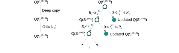
(a) The decision subtree for resource counter $r_{i}$

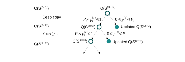
(b) The decision subtree for performance counter $p_{i}$

Figure 5: The decision subtree for resource or performance counters

We associate the execution of Algorithm 1, applied to $Q({\cal S})$, with a tree denoted by ${\cal T}(Q({\cal S}))$ and where both nodes and edges of ${\cal T}(Q({\cal S}))$ are labelled. We use the same notations as in Algorithm 2. We define ${\cal T}(Q({\cal S}))$ recursively:

We label the root of ${\cal T}(Q({\cal S}))$ with $Q({\cal S})$.

If ${\gamma}({\cal S})$ is empty, then ${\cal T}(Q({\cal S}))$ has no children; otherwise, two cases arise:

If no optimization strategy is to be applied for optimizing the counter $c$, then ${\cal T}(Q({\cal S}))$ has a single subtree, which is that associated with ${\sf Optimize}(Q({\cal S^{\prime}}))$ where $Q({\cal S^{\prime}})$ is obtained from $Q({\cal S})$ by augmenting $C({\cal S})$ either with $0\leq v_{i}\leq R_{i}$ if $c$ is a resource counter or with $0\leq v_{i}\leq{P}_{i}$ otherwise.

If an optimization strategy is applied, then ${\cal T}(Q({\cal S}))$ has two subtrees:

The first one is the tree associated with ${\sf Optimize}(Q({\cal S^{\prime}}))$ (where $Q({\cal S^{\prime}})$ is defined as above) and is connected to its parent node by the accept edge, labelled with either $0\leq v_{i}\leq R_{i}$ or $0\leq v_{i}\leq{P}_{i}$; see Figure 5.

The second one is the tree associated with ${\sf Optimize}(Q({\cal S^{\prime\prime\prime}}))$ (where $Q({\cal S^{\prime\prime\prime}})$ is obtained by applying the optimization strategy to the deep copy of the input quintuple $Q({\cal S})$) and is connected to its parent node by the refuse edge, labelled with either $R_{i}<v_{i}$ or ${P}_{i}<v_{i}\leq 1$; see Figure 5. Observe that every node of ${\cal T}(Q({\cal S}))$ is labelled with a quintuple and every edge with a polynomial constraint.

Figure 5 illustrates how Algorithm 2, applied to $Q({\cal S^{\prime}})$, generates the associated tree ${\cal T}(Q({\cal S^{\prime}}))$. The cases for a resource counter and a performance counter are distinguished in the sub-figures (a) and (b), respectively. Observe that, in both cases, the accept edges go south-east, while the refuse edges go south-west.

Input: The quintuple $Q({\cal S})$

Output: A comprehensive optimization of ${\cal S}$ w.r.t. the resource evaluation functions $f_{1},\ldots,f_{s}$, the performance evaluation functions $g_{1},\ldots,g_{t}$ and the optimization strategies $O_{1},\ldots,O_{w}$

if ${\gamma}({\cal S})$ is empty then  return $((G_{C}({\cal S}),{\lambda}({\cal S})),C({\cal S}))$;

 

The output stack is initially empty;

for each $Q({\cal S^{\prime}})\in{\sf Optimize}(Q({\cal S}))$ do  Push ${\sf ComprehensiveOptimization}(Q({\cal S^{\prime}})$ on the output stack;

 

return the output stack;

Algorithm 1 ComprehensiveOptimization

Input: A quintuple $Q({\cal S^{\prime}})$

Output: A stack of quintuples

Initialize an empty stack, called result;

Take out from ${\gamma}({\cal S^{\prime}})$ the next resource or performance counter to be evaluated, say $c$;

Evaluate $c$ on ${\cal S^{\prime}}$ (using the appropriate functions among $f_{1},\ldots,f_{s},g_{1},\ldots,g_{t}$) thus obtaining a value $v_{i}$, which can be either a numerical value, a polynomial in ${\mbox{${\mathbb{Q}}$}}[D_{1},\ldots,D_{u},E_{1},\ldots,E_{v}]$ or a rational function where its numerator and denominator are in ${\mbox{${\mathbb{Q}}$}}[D_{1},\ldots,D_{u},E_{1},\ldots,E_{v},$ $R_{1},\ldots,R_{s}]$;

if $c$ is a resource counter $r_{i}$ then  Make a deep copy $Q({\cal S^{\prime\prime}})$ of $Q({\cal S^{\prime}})$, since we are going to split the computation into two branches: $R_{i}<v_{i}$ and $0\leq v_{i}\leq R_{i}$;

Add the constraint $0\leq v_{i}\leq R_{i}$ to $C({\cal S^{\prime}})$ and push $Q({\cal S^{\prime}})$ onto result;

Add the constraint $R_{i}<v_{i}$ to $C({\cal S^{\prime\prime}})$ and search ${\omega}({\cal S^{\prime\prime}})$ for an optimization strategy of ${\sigma}(r_{i})$;

if no such optimization strategy exists then  return result;

  else  Apply such an optimization strategy to $Q({\cal S^{\prime\prime}})$ yielding $Q({\cal S^{\prime\prime\prime}})$;

Remove this optimization strategy from ${\omega}({\cal S^{\prime\prime\prime}})$;

if this optimization strategy is applied to the IR of ${\cal S^{\prime\prime}}$ then  Add it to ${\lambda}({\cal S^{\prime\prime\prime}})$;

  Push $r_{1},\ldots,r_{i-1},r_{i}$ onto ${\gamma}({\cal S^{\prime\prime\prime}})$;

Make a recursive call to Optimize on $Q({\cal S^{\prime\prime\prime}})$ and push the returned quintuples onto result;

    if $c$ is a performance counter $p_{i}$ then  Make a deep copy $Q({\cal S^{\prime\prime}})$ of $Q({\cal S^{\prime}})$, since we are going to split the computation into two branches: $0\leq v_{i}\leq{P}_{i}$ and ${P}_{i}<v_{i}\leq 1$ ;

Add the constraint $0\leq v_{i}\leq{P}_{i}$ to $C({\cal S^{\prime}})$ and push $Q({\cal S^{\prime}})$ onto result;

Add the constraint ${P}_{i}<v_{i}\leq 1$ to $C({\cal S^{\prime\prime}})$ and search ${\omega}({\cal S^{\prime\prime}})$ for an optimization strategy of ${\sigma}(p_{i})$;

if no such optimization strategy exists then  return result;

  else  Apply such an optimization strategy to $Q({\cal S^{\prime\prime}})$ yielding $Q({\cal S^{\prime\prime\prime}})$;

Remove this optimization strategy from ${\omega}({\cal S^{\prime\prime\prime}})$;

if this optimization strategy is applied to the IR of ${\cal S^{\prime\prime}}$ then  Add it to ${\lambda}({\cal S^{\prime\prime\prime}})$;

  Push $r_{1},\ldots,r_{s},p_{i}$ onto ${\gamma}({\cal S^{\prime\prime\prime}})$;

Make a recursive call to Optimize on $Q({\cal S^{\prime\prime\prime}})$ and push the returned quintuples onto result;

    Remove from result any quintuple with an inconsistent system of constraints;

return result;

Algorithm 2 Optimize

Lemma 1

The height of the tree ${\cal T}(Q({\cal S}))$ is at most $w(s+t)$. Therefore, Algorithm 1 terminates.

Proof $\rhd$ Consider a path $\Gamma$ from the root of ${\cal T}(Q({\cal S}))$ to any node $N$ of ${\cal T}(Q({\cal S}))$. Observe that $\Gamma$ counts at most $w$ refuse edges. Indeed, following a refuse edge decreases by one the number of optimization strategies to be used. Observe also that the length of every sequence of consecutive accept edges is at most $s+t$. Indeed, following an accept edge decreases by one the number of resource and performance counters to be evaluated. Therefore, the number of edges in $\Gamma$ is at most $w\,(s+t)$. $\lhd$

Lemma 2

Let $U:=\{U_{1},\ldots,U_{z}\}$ be a subset of $\{O_{1},\ldots,0_{w}\}$. There exists a path from the root of ${\cal T}(Q({\cal S}))$ to a leaf of ${\cal T}(Q({\cal S}))$ along which the optimization strategies being applied are exactly those of $U$.

Proof $\rhd$ Let us start at the root of ${\cal T}(Q({\cal S}))$ and apply the following procedure:

follow the refuse edge if it uses an optimization strategy from $\{U_{1},\ldots,U_{z}\}$,

follow the accept edge, otherwise. This creates a path from the root of ${\cal T}(Q({\cal S}))$ to a leaf with the desired property. $\lhd$

Definition 3

Let $i\in\{1,\ldots,s\}$ (resp. $\{1,\ldots,t\}$). Let $N$ be a node of ${\cal T}(Q({\cal S}))$ and $Q({\cal S}_{N})$ be the quintuple labelling this node. We say that $r_{i}$ (resp. $p_{i}$) is optimal at $N$ w.r.t. the evaluation function $f_{i}$ (resp. $g_{i}$) and the subset ${\sigma}(r_{i})$ (resp. ${\sigma}(p_{i})$) of the optimization strategies $O_{1},\ldots,O_{w}$, whenever for all $O\in{\sigma}(r_{i})$ (resp. ${\sigma}(p_{i})$) we have $f_{i}(O({\cal S}_{N}))=f_{i}({\cal S}_{N})$ (resp. $g_{i}(O({\cal S}_{N}))=g_{i}({\cal S}_{N})$).

Lemma 3

Let $i\in\{1,\ldots,s\}$ (resp. $\{1,\ldots,t\}$). There exists at least one leaf $L$ of ${\cal T}(Q({\cal S}))$ such that $r_{i}$ (resp. $p_{i}$) is optimal at $L$ w.r.t. the evaluation function $f_{i}$ (resp. $g_{i}$) and the subset ${\sigma}(r_{i})$ (resp. ${\sigma}(p_{i})$) of the optimization strategies $O_{1},\ldots,O_{w}$.

Proof $\rhd$ Apply Lemma 2 with $U={\sigma}(r_{i})$ (resp. $U={\sigma}(p_{i})$). $\lhd$

Lemma 4

Algorithm 1 satisfies its output specifications.

Proof $\rhd$ From Lemma 1, we know that Algorithm 1 terminates. So let $(C_{1},{\cal S}_{1}),\ldots,(C_{e},{\cal S}_{e})$ be its output. We shall prove $(C_{1},{\cal S}_{1}),\ldots,(C_{e},{\cal S}_{e})$ satisfies the conditions $(i)$ to $(iv)$ of Definition 2.

Condition $(i)$ is satisfied by the properties of the RealTriangularize algorithm. Condition $(ii)$ follows clearly from the assumption that the code transformations performed by $O_{1},\ldots,O_{w}$ preserve semantics. Observe that each time a polynomial inequality is added to a system of constraints, the negation of this inequality is also to the same system in another branch of the computations. By using a simple induction on $s+t$, we deduce that Condition $(iii)$ is satisfied. Finally, we prove Condition $(iv)$ by using Lemma 3. $\lhd$

4 Comprehensive Translation

Given a high-level model for accelerator programming (like OpenCL [23], OpenMP, OpenACC or MetaFork [11]), we consider the problem of translating a program written for such a high-level model into a programming model for GPGPU devices, such as CUDA. We assume that the numerical values of some, or all, of the hardware characteristics of the targeted GPGPU device are unknown. Hence, these quantities are treated as symbols. Similarly, we would like that some, or all, of the program parameters remain symbols in the generated code.

In our implementation, we focus on one high-level model for accelerator programming, namely MetaFork. However, we believe that an adaptation to another high-level model for accelerator programming would not be difficult. One supporting reason for that claim is the fact that automatic code translation between the MetaFork and OpenMP languages can already be done within the MetaFork compilation framework, see [11].

We consider as input a meta_schedule statement ${\cal M}$ and its surrounding MetaFork program ${\cal P}$. In our implementation, we assume that, apart from the meta_schedule statement ${\cal M}$, the rest of the program ${\cal P}$ is serial C code. Now, applying the comprehensive optimization algorithm (described in Section 3) on the meta_schedule statement ${\cal M}$ (with prescribed resource evaluation functions, performance evaluation functions and optimization strategies) we obtain a sequence of processed quintuples of meta_schedule statements ${\cal Q}_{1}({\cal M}),{\cal Q}_{2}({\cal M}),\ldots,{\cal Q}_{\ell}({\cal M})$, which forms a comprehensive optimization in the sense of Definition 2.

If, as mentioned in the introduction, PTX is used as intermediate representation (IR) then, for each $i=1,\ldots,{\ell}$, under the constraints defined by the polynomial system associated with ${\cal Q}_{i}({\cal M})$, the IR code associated with ${\cal Q}_{i}({\cal M})$ is the translation in assembly language of a CUDA counterpart of ${\cal M}$. In our implementation, we also translate to CUDA source code the MetaFork code in each ${\cal Q}_{i}({\cal M})$, since this is easier to read for a human being.

5 Experimentation

We report on a preliminary implementation of Algorithm 1 dedicated to the optimization of meta_schedule statements in view of generating parametric CUDA kernels. Two hardware resource counters are considered: register usage per thread, and local/shared memory allocated per thread-block. No performance counters are specified, however, by design, the algorithm tries to minimize the usage of hardware resources. Four optimization strategies are used: $(i)$ reducing register pressure, $(ii)$ controlling thread granularity, $(iii)$ common sub-expression elimination (CSE), and $(iv)$ caching data in local/shared memory. The first one applies to the IR CFG and uses LLVM; $(ii)$ and $(iii)$ are performed in Maple on the source CFG while $(iv)$ combines PET [26] and the RegularChains library in Maple. Moreover, for $(i)$ and $(iii)$, 3 and 2 levels of optimization are used, respectively. Figure 6 gives an overview of the software tools that are involved in our implementation.

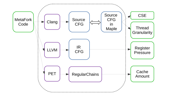
Figure 6: The software tools involved in our implementation

The test examples of our CASCON paper [9] have been extensively tested with that implementation. In the interest of space, we have selected two representative examples. For both of them, again in the interest of space, we present the optimized MetaFork code, instead of the optimized IR code (or the CUDA code generated from MetaFork).

For each system of constraints, we indicate which decisions were made by the algorithm to reach that case. To this end, we use the following abbreviations: (1), (2), (3a), (3b), (4a), (4b) respectively stand for “No register pressure optimization”, “CSE is Applied” “thread granularity not-reduced”, “reduced thread granularity”, “Use local/shared memory”, “Do not use local/shared memory”.

For both test-examples, we give speedup factors (against an optiimzied serial C code) obtained with the most efficient of our generated CUDA kernels. All CUDA experimental results are collected on an NVIDIA Tesla M2050.

5.1 1D Jacobi

Both source and optimized MetaFork programs are shown on Figure 7. Table 2 shows the speedup factors for the first case of optimized MetaFork programs in Figure 7.

Source code

int T, N, s, B,

int dim = (N-2)/(s*B);

int a[2*N];

for (int t = 0; t<T; ++t)

 meta_schedule {

  meta_for (int i = 0;

              i<dim; i++)

   meta_for (int j = 0;

                  j<B; j++)

    for (int k = 0; k<s;

                     ++k) {

     int p = i*s*B+k*B+j;

     int p1 = p + 1;

     int p2 = p + 2;

     int np = N + p;

     int np1 = N + p + 1;

     int np2 = N + p + 2;

     if (t % 2)

      a[p1] = (a[np]+

        a[np1]+a[np2])/3;

     else

      a[np1] = (a[p]+

        a[p1]+a[p2])/3;

    }

 }

First case

$\left\{\begin{array}[]{l}2sB+2\leq Z_{B}\\ 9\leq R_{B}\\ \end{array}\right.$

(1) (4a) (3a) (2) (2)

for (int t = 0; t<T; ++t)

 meta_schedule cache(a) {

  meta_for (int i = 0;

              i< dim; i++)

   meta_for (int j = 0;

                  j<B; j++)

    for (int k = 0; k<s;

                     ++k) {

     int p = j+(i*s+k)*B;

     int t16 = p+1;

     int t15 = p+2;

     int p1 = t16;

     int p2 = t15;

     int np = N+p;

     int np1 = N+t16;

     int np2 = N+t15;

     if (t % 2)

      a[p1] = (a[np]+

        a[np1]+a[np2])/3;

     else

      a[np1] = (a[p]+

        a[p1]+a[p2])/3;

     }

 }

Second case

$\left\{\begin{array}[]{l}2B+2\leq Z_{B}\\ Z_{B}<2sB+2\\ 9\leq R_{B}\\ \end{array}\right.$

(1) (3b) (4a) (3a) (2) (2)

for (int t = 0; t<T; ++t)

 meta_schedule cache(a) {

  meta_for (int i = 0;

              i<dim; i++)

   meta_for (int j = 0;

                j<B; j++) {

    int p = i*B+j;

    int t20 = p+1;

    int t19 = p+2;

    int p1 = t20;

    int p2 = t19;

    int np = N+p;

    int np2 = N+t19;

    int np1 = N+t20;

    if (t % 2)

     a[p1] = (a[np]+

       a[np1]+a[np2])/3;

    else

     a[np1] = (a[p]+

       a[p1]+a[p2])/3;

    }

 }

Third case

$\left\{\begin{array}[]{l}Z_{B}<2B+2\\ 9\leq R_{B}\\ \end{array}\right.$

(1) (3b) (2) (2) (4b)

for (int t = 0; t<T; ++t)

 meta_schedule {

  meta_for (int i = 0;

              i<dim; i++)

   meta_for (int j = 0;

                j<B; j++) {

    int p = j+i*B;

    int t16 = p+1;

    int t15 = p+2;

    int p1 = t16;

    int p2 = t15;

    int np = N+p;

    int np1 = N+t16;

    int np2 = N+t15;

    if (t % 2)

     a[p1] = (a[np]+

       a[np1]+a[np2])/3;

    else

     a[np1] = (a[p]+

       a[p1]+a[p2])/3;

    }

 }

Figure 7: Three optimized MetaFork programs for 1D Jacobi

Thread-block $\backslash$ Granularity	2	4	8
16	3.340	4.357	4.975
32	4.785	5.252	5.206
64	5.927	6.264	6.412
128	10.400	8.952	5.793
256	6.859	6.246

Table 2: Speedup factors of 1D Jacobi for time iteration 4 and input vector of length $2^{15}$+2

5.2 Matrix transposition

Three cases of optimized MetaFork programs are shown on Figure 8. Table 3 shows the speedup factors for the first case of optimized MetaFork programs in Figure 8.

First case

$\left\{\begin{array}[]{l}2sB_{0}B_{1}\leq Z_{B}\\ 6\leq R_{B}\\ \end{array}\right.$

(1) (4a) (3a) (2) (2)

meta_schedule cache(a, c) {

 meta_for (int v0 = 0; v0<dim0; v0++)

  meta_for (int v1 = 0; v1<dim1; v1++)

   meta_for (int u0 = 0; u0<B0; u0++)

    meta_for (int u1 = 0; u1<B1; u1++)

     for (int k = 0; k < s; ++k) {

      int i = v0*B0+u0;

      int j = (v1*s+k)*B1+u1;

      c[i*N+j] = a[i][j];

     }

}

Second case

$\left\{\begin{array}[]{l}2B_{0}B_{1}\leq Z_{B}\\ Z_{B}<2sB_{0}B_{1}\\ 5\leq R_{B}\\ \end{array}\right.$

(1) (3b) (4a) (3a) (2) (2)

$\left\{\begin{array}[]{l}2B_{0}B_{1}\leq Z_{B}\\ Z_{B}<2sB_{0}B_{1}\\ 5\leq R_{B}<6\\ \end{array}\right.$

(2) (2) (3b) (1) (4a) (3a)

meta_schedule cache(a, c) {

 meta_for (int v0 = 0; v0<dim0; v0++)

  meta_for (int v1 = 0; v1<dim1; v1++)

   meta_for (int u0 = 0; u0<B0; u0++)

    meta_for (int u1 = 0; u1<B1; u1++) {

     int i = v0*B0+u0;

     int j = v1*B1+u1;

     c[i*N+j] = a[i][j];

    }

}

Third case

$\left\{\begin{array}[]{l}Z_{B}<2B_{0}B_{1}\\ 5\leq R_{B}\\ \end{array}\right.$

(1) (3b) (2) (2) (4b)

$\left\{\begin{array}[]{l}Z_{B}<2B_{0}B_{1}\\ 5\leq R_{B}<6\\ \end{array}\right.$

(2) (2) (3b) (1) (4b)

meta_schedule {

 meta_for (int v0 = 0; v0<dim0; v0++)

  meta_for (int v1 = 0; v1<dim1; v1++)

   meta_for (int u0 = 0; u0<B0; u0++)

    meta_for (int u1 = 0; u1<B1; u1++) {

     int i = v0*B0+u0;

     int j = v1*B1+u1;

     c[i*N+j] = a[i][j];

    }

}

Figure 8: Three optimized MetaFork programs for matrix transposition

Thread-block $\backslash$ Granularity	2	4	8
(4, 32)	103.281	96.284	75.211
(8, 32)	111.971	90.625	85.422
(16, 32)	78.476	68.894	48.822
(32, 32)	45.084	46.425	32.824

Table 3: Speedup factors of matrix transposition for input matrix of order $2^{14}$

6 Concluding Remarks

We have shown how, from an annotated C/C++ program, parametric CUDA kernels could be optimized. These optimized parametric CUDA kernels are organized in the form of a case discussion, where cases depend on the values of machine parameters (e.g. hardware resource limits) and program parameters (e.g. dimension sizes of thread-blocks).

The proposed approach extend previous works, in particular PPCG [25] and CUDA-CHiLL [16], and combine them with techniques from computer algebra. Indeed, handling systems of non-linear polynomial equations and inequalities is required in the context of parametric CUDA kernels.

Our preliminary implementation uses LLVM, Maple and PPCG; it successfully processes a variety of standard test-examples. In particular, the computer algebra portion of the computations is not a bottleneck.

References

- [1] User guide for NVPTX. The LLVM Compiler Infrastructure. http://llvm.org/docs/NVPTXUsage.html#introduction.
- [2] CUDA runtime API: v7.5. NVIDIA Corporation, 2015. {http://docs.nvidia.com/cuda/pdf/CUDA_Runtime_API.pdf}.
- [3] The OpenACC application programming interface. OpenACC-Standard.org, 2015.
- [4] OpenMP application program interface version 4.5. OpenMP Architecture Review Board, 2015. http://www.openmp.org/mp-documents/openmp-4.5.pdf.
- [5] Parallel thread execution ISA : v4.3. NVIDIA Corporation, 2015. http://docs.nvidia.com/cuda/pdf/ptx_isa_4.3.pdf.
- [6] Ravi Sethi Aho, Alfred V. and Jeffrey D. Ullman. Compilers: Principles, Techniques and Tools. Addison-Wesley, Reading, Massachusetts, 2006.
- [7] M. Baskaran, J. Ramanujam, and P. Sadayappan. Automatic C-to-CUDA code generation for affine programs. In Proceedings of CC’10/ETAPS’10, pages 244–263, Berlin, Heidelberg, 2010. Springer-Verlag.
- [8] Carlo Bertolli, Samuel F. Antao, Alexandre E. Eichenberger, Kevin O’Brien, Zehra Sura, Arpith C. Jacob, Tong Chen, and Olivier Sallenave. Coordinating GPU threads for OpenMP 4.0 in LLVM. In Proceedings of LLVM-HPC ’14, pages 12–21. IEEE Press, 2014.
- [9] Changbo Chen, Xiaohui Chen, Abdoul-Kader Keita, Marc Moreno Maza, and Ning Xie. MetaFork: A compilation framework for concurrency models targeting hardware accelerators and its application to the generation of parametric CUDA kernels. In Proceedings of CASCON 2015, pages 70–79, 2015.
- [10] Changbo Chen, James H. Davenport, John P. May, Marc Moreno Maza, Bican Xia, and Rong Xiao. Triangular decomposition of semi-algebraic systems. J. Symb. Comput., 49:3–26, 2013.
- [11] Xiaohui Chen, Marc Moreno Maza, Sushek Shekar, and Priya Unnikrishnan. MetaFork: A framework for concurrency platforms targeting multicores. In Processing of IWOMP 2014, pages 30–44, 2014.
- [12] Leonardo Dagum and Ramesh Menon. OpenMP: An industry standard API for shared-memory programming. Computational Science & Engineering, IEEE, 5(1):46–55, 1998.
- [13] Matteo Frigo and Steven G. Johnson. FFTW: an adaptive software architecture for the FFT. In Proceedings of ICASSP, pages 1381–1384. IEEE, 1998.
- [14] Scott Grauer-Gray, Lifan Xu, Robert Searles, Sudhee Ayalasomayajula, and John Cavazos. Auto-tuning a high-level language targeted to GPU codes. In Innovative Parallel Computing. IEEE, 2012.
- [15] Tianyi David Han and Tarek S. Abdelrahman. hiCUDA: A high-level directive-based language for GPU programming. In Proceedings of GPGPU-2, pages 52–61. ACM, 2009.
- [16] Malik Khan, Protonu Basu, Gabe Rudy, Mary Hall, Chun Chen, and Jacqueline Chame. A script-based autotuning compiler system to generate high-performance CUDA code. ACM Trans. Archit. Code Optim., 9(4):31:1–31:25, January 2013.
- [17] Thomas Kistler and Michael Franz. Continuous program optimization: A case study. ACM Trans. on Programming Languages and Systems, 25(4):500–548, 2003.
- [18] Chris Lattner and Vikram Adve. LLVM: A compilation framework for lifelong program analysis & transformation. In Proceedings of CGO ’04, pages 75–. IEEE Computer Society, 2004.
- [19] J. Nickolls, I. Buck, M. Garland, and K. Skadron. Scalable parallel programming with CUDA. Queue, 6(2):40–53, 2008.
- [20] Markus Püschel, José M. F. Moura, Bryan Singer, Jianxin Xiong, Jeremy R. Johnson, David A. Padua, Manuela M. Veloso, and Robert W. Johnson. Spiral: A generator for platform-adapted libraries of signal processing alogorithms. IJHPCA, 18(1), 2004.
- [21] Helge Rhodin. A PTX code generator for LLVM. Master’s thesis, Saarland University, 2010.
- [22] Chenchen Song, Lee-Ping Wang, and Todd J Martínez. Automated code engine for graphical processing units: Application to the effective core potential integrals and gradients. Journal of chemical theory and computation, 2015.
- [23] J. E Stone, D. Gohara, and G. Shi. OpenCL: A parallel programming standard for heterogeneous computing systems. Computing in science & engineering, 12(3):66, 2010.
- [24] Xiaonan Tian, Rengan Xu, Yonghong Yan, Zhifeng Yun, Sunita Chandrasekaran, and Barbara M. Chapman. Compiling a high-level directive-based programming model for GPGPUs. In Languages and Compilers for Parallel Computing - 26th Int. Work. Springer, 2013.
- [25] S. Verdoolaege, J. Carlos Juega, A. Cohen, J. Ignacio Gómez, C. Tenllado, and F. Catthoor. Polyhedral parallel code generation for CUDA. TACO, 9(4):54, 2013.
- [26] Sven Verdoolaege and Tobias Grosser. Polyhedral extraction tool. In Second International Workshop on Polyhedral Compilation Techniques (IMPACT 2012), Paris, France, 2012.
- [27] R. Clinton Whaley and Jack Dongarra. Automatically tuned linear algebra software. In PPSC, 1999.