Predicting Future Lane Changes of Other Highway Vehicles using RNN-based Deep Models
Abstract
In the event of sensor failure, autonomous vehicles need to safely execute emergency maneuvers while avoiding other vehicles on the road. To accomplish this, the sensor-failed vehicle must predict the future semantic behaviors of other drivers, such as lane changes, as well as their future trajectories given a recent window of past sensor observations. We address the first issue of semantic behavior prediction in this paper, which is a precursor to trajectory prediction, by introducing a framework that leverages the power of recurrent neural networks (RNNs) and graphical models. Our goal is to predict the future categorical driving intent, for lane changes, of neighboring vehicles up to three seconds into the future given as little as a one-second window of past LIDAR, GPS, inertial, and map data.
We collect real-world data containing over 20 hours of highway driving using an autonomous Toyota vehicle. We propose a composite RNN model by adopting the methodology of Structural Recurrent Neural Networks (RNNs) to learn factor functions and take advantage of both the high-level structure of graphical models and the sequence modeling power of RNNs, which we expect to afford more transparent modeling and activity than opaque, single RNN models. To demonstrate our approach, we validate our model using authentic interstate highway driving to predict the future lane change maneuvers of other vehicles neighboring our autonomous vehicle. We find that our composite Structural RNN outperforms baselines by as much as 12% in balanced accuracy metrics.
I Introduction
Autonomous vehicles are equipped with many advanced sensors that allow them to perceive other vehicles, obstacles, and pedestrians in the environment. Substantial work has been done in the areas of perception and reasoning for autonomous vehicles and other forms of robots to allow these agents to make decisions based on their percepts [1, 2]. However, the majority of this past work make the tacit assumption that the sensors are working reliably. Hence, in these systems, the ability to make autonomous decisions is lost under sensor failure. In practice, such an assumption is risky and not always a guarantee, especially in the case of autonomous vehicles deployed in the real world amongst other human-driven vehicles. In the event of sensor failure in autonomous vehicles, only past sensor readings are available for decision making. These vehicles then need to be able to plan and execute emergency maneuvers while safely avoiding other moving obstacles on the road.
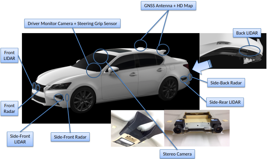
To optimally execute emergency maneuvers requires the knowledge of what other vehicles surrounding the blinded agent are going to do in the near future, including predicting semantic maneuvers and exovehicle111Throughout the paper, we use the term exovehicles to refer to the vehicles in the vicinity of our autonomous vehicle, which we refer to as the egovehicle. trajectories. In this work, we specifically address the first issue of predicting the maneuvers of other vehicles up to three seconds into the future, such as performing left or right lane change maneuvers or staying in the same lane, while driving on the highway. Since future exovehicle trajectories are dependent on these semantic behaviors, tackling the behavior prediction problem becomes a necessary prerequisite that can simplify the trajectory prediction problem. We approach this problem using as little as one-second and up to five-seconds of past observations of neighboring vehicles based on LIDAR, GPS, inertial, and high-definition map data collected from an autonomous Toyota vehicle (see Fig. 1).
There are two distinct categories of modeling choices for this problem of predicting semantic categories of exovehicle behavior: a classical probabilistic graphical modeling [5] approach and a contemporary deep neural network [6, 7] approach. Both approaches are able to integrate various measurements into a common representation and to model their temporal evolution.
The classical approach of probabilistic graphical models [5], such as factor graphs, spatiotemporal graphs, and dynamic Bayesian networks [8], which bring graphical models into the sequential modeling space, is widely used in the robotics community for many reasons, including their interpretability and the high level structures, which can capture various relationships between features to modeling temporal sequences. However, they require a parameterization of factor models that is structured by hand using domain-specific knowledge and optimized using various methods, including structural support vector machines and expectation maximization [9], which, arguably, struggle to incorporate large-scale data well.
On the other hand, recent advancements in temporal sequence modeling have come from the use of recurrent neural networks (RNNs) [6, 7], which can be trained end-to-end for various tasks. While methods that rely on deep learning lack the interpretability of factor graphs, these networks learn richer models than those currently employed in factor graphs. Indeed, RNN-based methods have been applied to predicting future vehicle maneuvers but only in the context of making predictions for a single observed human driver [10, 11].
In this work, we want both the interpretability of factor graphs and the scalability of deep RNNs. To that end, we bring RNN-based methods to the problem of predicting the future maneuvers of exovehicles within the vicinity of our own autonomous vehicle while traveling on a highway. We propose a composite RNN that leverages the recent work in Structural RNNs (SRNNs) [11]. Here, RNN units are connected in the form of factor graphs. These networks employ the interpretable, high-level spatiotemporal structure of graphical models while using RNN units specifically to learn rich, nonlinear factor and node functions for factor graphs. As with single RNN-based networks, SRNNs are trained end-to-end and can be unrolled over each step in the temporal sequence at inference time to make the predictions for the given task. Following the methodology of SRNNs, we propose a novel lane-based graphical model which we then convert into a SRNN so we can learn rich factor models for lane change prediction.
Our composite lane SRNN captures the spatiotemporal interactions between a given vehicle and its neighbors in the same and adjacent lanes. To model lane-wise interactions, the graph includes a factor for the right, left, and same lanes that combines pose, velocity, and map-based lane information for the neighboring vehicles within the given lane. The model is unrolled over each time step of the sequence of past sensor observations to predict the future lane change maneuver class.
We provide an analysis on the efficacy of our lane-based SRNN in predicting the future behavior of all tracked highway vehicles in alternative lanes, not just forward and backward in the same lane, in the event of sensor malfunction for varying future and past time horizons. We train and evaluate our models using natural multi-lane interstate highway driving data obtained from an autonomous vehicle driving amongst other human drivers. This data set is not augmented with simulated driving scenarios as in Galceran et al., 2015 [4] and is more extensive than other highway datasets used in Jain et al., 2016 [10]. Thus, the performance of our models on this data set constitutes the performance of our models on the actual autonomous robot for authentic highway driving.
II Related Works
II-A Maneuver Anticipation
Recent work in predicting driver maneuvers has primarily focused on the intent of the target vehicle’s human driver; intent is based on tracking the driver’s face with an inward-facing camera along with features outside of and in front of the vehicle using a camera, velocity sensor, and GPS [11, 10, 9]. The works of Jain et al., 2016 [11, 10] use various RNN-based architectures while Jain et al., 2015 uses graphical models [9], both of which are essential to this work. However, rather than anticipating the behavior of our own vehicle, we address the problem of predicting the lane change maneuvers of neighboring vehicles in an interstate highway environment. Moreover, by utilizing a multi-LIDAR system that provides all-around coverage, we predict future maneuvers for multiple vehicles in the surrounding neighborhood rather than only those detected and tracked in front of the data collection (ego) vehicle.
The method in Galceran et al., 2015 [4] involves anticipating the maneuvers of other vehicles and takes a reinforcement learning approach to simulate multiple possible future maneuvers. While it chooses the ones that are most likely to occur; however, this approach is based on simulated approximations of limited highway driving scenarios. Conversely, our method is trained and evaluated on data collected from natural freeway driving, which keeps our validation unaffected by simulation-based modeling errors.
II-B Graphical Models and Structural RNNs
Graphical models are used in Jain et al., 2015 [9] in the form of autoregressive input-output Hidden Markov Models (HMMs) to model the temporal sequences that lead up to various maneuvers. Similarly, HMMs are used in Schlechtriemen et. al, 2014 [12], using a similar neighborhood context for the target vehicle; however, this method relies on hand-tuned features computed from the tracked poses and map information of all of the vehicles rather than learning the factor models without restrictive assumptions on what features to extract. The work presented in Jain et al., 2016 [11] bridges the gap between probabilistic graphical models and deep learning by introducing the Structural RNN, which exhibits better performance over graphical model counterparts through evaluations in many problem spaces, including maneuver anticipation for the target vehicle’s human driver using facial tracking. While our method follows the same methodology of transforming a graph into a Structural RNN, we propose a novel graph that takes into account lane-based spatiotemporal interactions between vehicles in the neighborhood of the target vehicle to predict future lane change maneuvers. We also evaluate the performance solely on natural freeway driving rather than city driving.
III Problem Set-Up and Data
Given a recent history of sensor readings varying from one to five seconds, our goal is to predict the lane-changing behavior of exovehicles at prediction horizons varying from seconds to seconds. Our prediction space is either left-lane change, right-lane change, or no-lane change. We collect a data set of highway driving using a Toyota sedan retrofitted with the sensors of a typical automated vehicle. In this paper, we will refer to this vehicle as the egovehicle, shown in Figure 1. The sensor suite includes 6 ibeo LUX 4L LIDARs mounted on all sides of the ego vehicle as well as an Applanix POS LV (version 5) high-accuracy GPS with Real-Time Kinetic (RTK) corrections. Using the ibeo LUX Fusion System [13], we detect the relative position and orientation of neighboring vehicles up to approximately meters away.
Using high-definition maps that include lane-level information (e.g. lane widths, markings, curvature, GPS coordinates, etc.) along with GPS measurements and the relative detections of neighboring vehicles, we localize the ego vehicle and its neighbors on the map. The GPS coordinates of the ego vehicle are projected into a world-fixed frame using the Mercator projection [14], and the relative poses of other vehicles are also mapped into this frame to determine absolute poses. Similarly, the velocities and yaw rates of all vehicles are determined. Along with vehicle poses, the maps allow us to determine the lane in which the ego and neighboring vehicles are traveling in. Over 20 hours of this data are collected at 12.5 Hz on multi-lane highways in Southeast Michigan and Southern California, giving us roughly 1 million samples for behavior prediction.
Given these off-the-shelf methods for detecting other vehicles and localizing them to the map, we focus on developing a framework that uses pose, velocity, and lane information to predict future lane changes. Specifically, we represent the vehicle at each time step with the following state vector:
| (1) |
where and are the absolute world-fixed frame positions in meters and and are their velocities, is the heading angle of the vehicle in radians with as the yaw rate in radians/second, is the number of lanes to the left of the vehicle, and is the number of lanes to the right of the vehicle (both in the direction of travel). We represent the sequence of historical states over time for each vehicle as
| (2) |
where is the maximum number of historical time steps included. For each vehicle at each time step, there are three possible lane change maneuvers that can occur time steps into the future222We use 7 steps to represent 0.5 seconds. Since the data frequency is 12.5 Hz, we round all fractional steps up to the nearest integer. –left-lane change, right-lane change, and no-lane change. We denote this set of possible maneuvers as . These are determined by examining the change in lane identifiers provided in the map between times and . We represent these labels as one-hot vectors in (1) and annotate each vehicle state in (2) with its future lane change label vector.
IV Lane Change Prediction Model
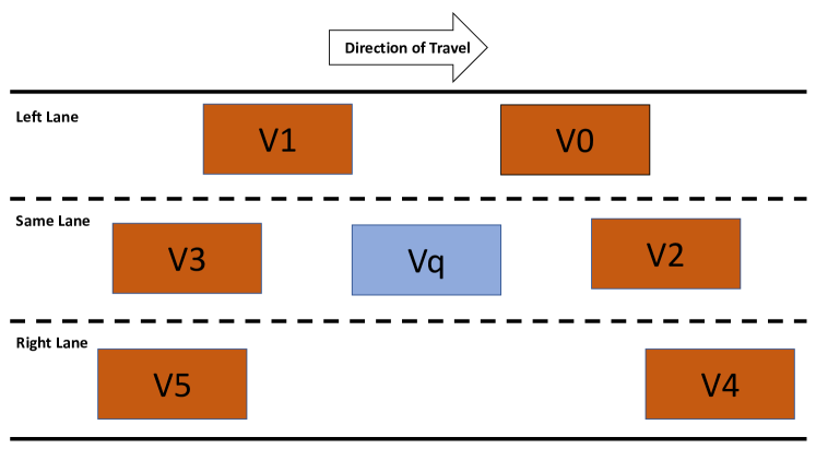
In this section, we discuss our proposed composite lane SRNN model, which allows us to transparently model that problem using factor graphs and, at the same time, compose the factors together into an RNN-based model. For a given exovehicle traveling on a multi-lane highway, we model the future lane change probability as a function of the vehicle’s previous states as well as the previous states of its neighboring vehicles. We use a six-vehicle neighborhood, shown in Fig. 2, that contains the vehicles ahead and behind the target vehicle in the left and right lanes and the vehicles directly ahead and behind the target vehicle in the same lane. According to this convention, for every target vehicle , the neighbors ahead and behind it in the left lane are and , the neighbors ahead and behind it in the same lane are and , and the neighbors ahead and behind it in the right lane are and .
Since may be at the right- or left-most lane or other vehicles may be out of sensor range during natural freeway driving, it is not guaranteed that each of these neighboring positions is actually occupied by a vehicle. For this reason, we only include a neighborhood of six vehicles, which provides a minimalist representation of the target vehicle’s context. Accordingly, we augment the state of each neighboring vehicle from each time step to with an indicator variable of 1 for when it is present in the target vehicle’s neighborhood and 0 for when it is not. We use these augmented neighbor vehicle states as well as the target vehicle’s state as the inputs to our lane change prediction model.
IV-A Graphical Models for Lane-Based Maneuver Prediction
Given the three-lane structure of the target vehicle’s neighborhood, we design a factor graph that represents the probability of the future lane change label of the target vehicle using edges that represent the interaction between vehicles in each lane (left, same, right) with the target vehicle. We make the assumption that given the observed state of the target vehicle at a given time step, the states of vehicles in a given lane are conditionally independent of vehicles in other lanes at that time step. Hence, we model factors for vehicles in the left, right, and same lanes separately. Furthermore, we assume that the target vehicle behavior is conditioned on the states of the vehicles within the three-lane context. The random variables are the target vehicle behavior labels and the future vehicle states; however, only the future behavior label is of interest. We start with the joint distribution over the target vehicle’s behavior labels and the states of all vehicles within the context from times to , and we use our assumptions to model the probability of the label taking on value as follows:
| (3) | ||||
We further factorize the distributions in (3) based on our assumption of conditional independence between lanes and Markovian temporal dynamics:
| (4) | ||||
| (5) | ||||
where each function and is a parameterization of the spatiotemporal and temporal factor functions, respectively, and where , , denote the left, right, and same lanes. These functions can take on various forms, include exponential models in the case of the spatiotemporal factors and Gaussians in the case of the temporal models [5]. By parameterizing each of the three lane factors using the states of each of the neighboring cars in the lane along with the target vehicle, we allow the model to take into account spatiotemporal interactions between each of the vehicles used in each factor. Hence, from the vehicle states for a given lane, we can accommodate the possibility of using relative distance and velocity features between vehicles. The final lane change prediction is given by
| (6) |
IV-B Learning Factor Functions using Structural RNNs
Factor functions are typically parameterized by hand to incorporate hand-tuned features with simple weights, which limits the modeling power of standard factor graphs [11, 10, 15]. Following the approach of Jain et al., 2016 [11], we preserve the transparency of the graphical model and, yet, leverage the power of RNNs by converting it into a Structural RNN (SRNN) trained to classify the lane change label. The SRNN composites factors, captured as network snippets, into a larger RNN. Specifically, random variable and factor nodes within graphical models are represented using their own RNN units (which we will call nodeRNNs and factorRNNs, respectively). This allows us to use the sequence modeling power of RNNs together with the structure provided by our spatiotemporal factor graph.
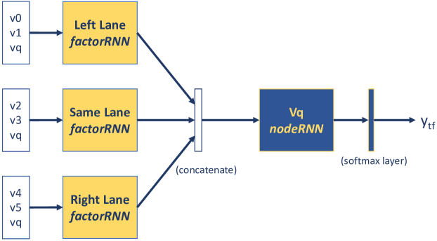
To convert our graph into a Structural RNN, we use LSTM units to represent each of the three lane interaction factors (each in (4)) as factorRNNs. While standard Structural RNNs use different LSTM units for each spatiotemporal and temporal factor as in Jain et al., 2016 [11], we note that a single LSTM unit can jointly model both the spatiotemporal factors along with temporal factors (each in (5)) for a given lane. LSTM units have two recurrent functions within them–one for computing the output and one for computing the context vector at each time step given the input features and previous outputs and states [7]. We provide extra details about the LSTM unit in Appendix A. This allows us to model the spatiotemporal interaction factors with the recurrent output function since the outputs of those are directly used in the prediction of the future lane change label. Similarly, we use the recurrent context vector function within each LSTM to model temporal factors as a function of the input vehicle states. By using a single LSTM to model both factors for each lane, we reduce the complexity of our model and benefit from being able to train it with a smaller dataset.
Since our graph has a single random variable node representing the future lane change maneuver, our Structural RNN has one nodeRNN to combine the outputs of each lane’s factorRNN. During the forward pass of the Structural RNN, each lane’s vehicle state at each time step are passed through their respective factorRNNs. The outputs of the three factorRNNs are then concatenated passed through the nodeRNN. The following equations detail the computation performed at each time step, noting that represents the LSTM model (model details are provided in Appendix A), and are the hidden outputs and context vectors, respectively, of the LSTM unit at time step , and that the scripts and mean left lane, right lane, same lane, and node, respectively:
| (7) | ||||
| (8) | ||||
| (9) | ||||
| (10) |
where all and are zero initialized before each forward pass through the network. After unrolling all time steps of vehicle states through the Structural RNN, we take the nodeRNN’s output of the last time step and pass it through a softmax layer to obtain the final lane change prediction for the target vehicle as follows:
| (11) |
where and are the weights and bias of the fully connected layer that transforms the output into the log-probabilities fed into the softmax function [16, 17].
At inference time, we use the final time step’s output of the Structural RNN as the future lane change prediction; however, during end-to-end training, we follow the approach of Jain et al., 2016 [10] and apply a time-based, exponentially weighted softmax cross-entropy loss function to each time step’s output, whereby outputs of the network early on are weighted less while outputs toward the end of the input sequence are weighted more. This encourages the model to predict the label at all time steps while penalizing early outputs less since they are only based on the early portion of the RNN input sequence. Doing so leads to better recurrent outputs being used to build up to the final lane change prediction.
IV-C Implementation Details
Our proposed lane-based SRNN model is implemented using LSTMs with layer normalization [18]. All LSTM units within the SRNN have a hidden state size of 128. The fully connected layer has an input size of 128 and output size of . During training, we use 50% weight dropout in the LSTM units as implemented in Semeniuta et al., 2016 [19]. We optimize the exponentially weighted softmax cross-entropy loss using the ADAM optimizer [20] with a learning rate of . In addition, we center and scale the vehicle state inputs to have zero mean and unit variance as a part of our preprocessing step. All of our software is implemented in Python using Tensorflow [21].
V Experiments
V-A Setup
We use the data set collected by our autonomous vehicle (Sec. III) for evaluation. For a given time history and future prediction horizon, we sample all the target vehicles tracked long enough to satisfy these time requirements and split up the data set into a training and evaluation set that contains 60% and 40% of the entire data, respectively. In natural freeway driving scenarios, no-lane change events outnumber the number of left-lane and right-lane change events; thus, we manually balance each training set to contain equal numbers of left-lane, right-lane, and no-lane change samples. We use the authentic, unbalanced evaluation set to test our models.
Each sample is pre-processed to center the initial target vehicle position and orientation at the origin of a fixed reference frame. This is done using applying a 2D rotation by the target vehicle’s initial yaw and a translation by its initial position coordinate to all vehicle positions (for target and neighbors). The initial target vehicle yaw is subtracted for all vehicles as well, and all velocities are rotated accordingly. Following this step, we center the training data and scale it to have zero mean and unit norm before passing the data as input to the lane change prediction model.
To evaluate the performance of our methods for various time horizons, we train our lane-based SRNN and baseline models (Sec. V-B) from scratch for each setting of time history and future prediction horizon . In our experiments, we choose 1, 3, and 5 seconds for 333These correspond to 13, 38, and 63 time steps, respectively when accounting for the data frequency of 12.5 Hz. and 1, 2, and 3 seconds for 444Similarly, these correspond to 13, 25, and 38 time steps, respectively..
V-B Baseline Methods
We compare our lane-based SRNN to three types of baseline models–classical Hidden Markov models (HMMs), single LSTM models, and a simpler, single-factor SRNN. Since our method comes about from a temporal graphical model, we first compare it against the classical approach using Hidden Markov models (HMM) [17]. Each of the three behaviors is modeled using its own HMM with multivariate Gaussian emission probabilities. All the vehicle states (for neighbors and the target vehicle) are concatenated together to create a single observation vector per time step. The HMMs are then trained in an unsupervised manner on training data specific to their lane change class. At inference time, the forward passes of the three HMMs are applied to the input sequence in parallel to produce class probabilities, and the class with the highest (normalized) probability is chosen as the final prediction. We choose the number of latent states for each maneuver’s HMM to maximize the overall f1 score (harmonic mean of precision and recall) across the three manuevers in a grid search evaluated on 20% of the training data withheld for a validation set.
Since our method is composed of multiple LSTM units, we compare it against a prediction model that uses only one LSTM unit. This can also be viewed as having only a nodeRNN present. To further evaluate the effect of our novel three-lane structure used in the SRNN, we compare our method against a simpler, single-factor SRNN where we only use one factorRNN instead of three. The output of this single factorRNN is fed directly as input to the nodeRNN. This is akin to using a stacked LSTM for lane change prediction.
For both LSTM baselines, we use the same type of LSTM units with hidden state sizes of 128 and layer normalization as we do with our lane SRNN method. The outputs at each time step of both models are also passed through the same size 128x3 fully connected layer and the softmax function to produce the lane change probabilities. At inference time, only the last time step’s output is used to make a future lane change prediction. As with the HMM model, we concatenate all the vehicle states together per time step to feed as input to the model. We train each LSTM baseline end-to-end using the exponentially weighted softmax loss function applied to all time steps, 50% recurrent dropout, and the same learning rate of as with our lane SRNN.
V-C Evaluation Metrics
We evaluate each model using precision, recall, and accuracy for predicting left, right, and no lane change behaviors for our proposed model and baselines evaluated on authentic highway driving. We compute the number of true positives , false positives , and false negatives for each maneuver . We use these to compute the precision and recall values as and , respectively. We also calculate the overall prediction accuracy of the models, although it is not very useful since the vast majority of the cases are no-lane change. To overcome this limitation, we calculate two other summary measures–balanced accuracy and positive lane-change accuracy. The balanced accuracy is a class averaged accuracy over the three cases, equally weighting the left-lane, right-lane and no-lane change accuracies. The positive lane-change accuracy is the accuracy for the subset of the evaluation data with the no-lane change samples completely discarded.
VI Analysis
We focus our analysis on the summary measures involving the various accuracy metrics; however, we provide the full results for each evaluation metric (Sec V-C) in Table II in Appendix B.
| Model | Avg Acc | Avg PLC Acc | Avg Bal Acc |
|---|---|---|---|
| HMM | 0.090 | 0.485 | 0.372 |
| Single LSTM | 0.158 | 0.433 | 0.376 |
| Single-Factor SRNN | 0.140 | 0.441 | 0.365 |
| Lane SRNN (ours) | 0.144 | 0.487 | 0.392 |
Note: Acc refers to overall accuracy; PLC Acc refers to positive lane-change accuracy; Bal Acc refers to balanced accuracy.
VI-A Holistic Performance
To analyze how the models perform as a whole, we average the accuracy metrics provided in Table II and present them in Table I. We see that for average positive lane-change and balanced accuracies, our lane SRNN outperforms all baselines. The single LSTM does have a better average overall accuracy; however, this comes at the expense of missing the predictions of future lane changes while predicting no-lane change behavior slightly better than the other models. Even in this case, our lane SRNN is the second-best performing method, showing that it still has benefits over the single-factor SRNN and the classical HMM baseline. In general, all models are affected by false positives where no-lane change samples are incorrectly predicted as left or right lane changes. This is a result of the skewed class representation in authentic driving and leads to relatively small overall accuracies on the evaluation data.
VI-B Comparison of RNN-based Methods Against HMMs
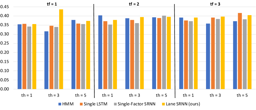
From our time horizon experiments, we see a consistent trend in the performance of our Lane SRNN, as well as the RNN baselines, against the classical HMM method with respect to balanced accuracies shown in Fig 4. As both the future prediction horizon and time history increases, the RNN-based methods increasingly do better than HMMs. We see the largest performance different for the case of and where our lane SRNN outperforms the HMM by 12% in balanced accuracy. In the extreme case of predicting lane changes 3 seconds into the future given 5 seconds of history, RNN-based models outperform HMMs by as much as 4%. HMMs are limited in their ability to capture intricate temporal lane change models with only multivariate Gaussian emissions and log-linear transition probabilities. Conversely, we see that our RNN-based methods are able to learn richer temporal models over longer sequences of time history that lead to thier observed higher performance.
VI-C Comparison of Lane SRNN to RNN Baselines
From the balanced accuracy results displayed in Fig. 4, we see that our proposed lane SRNN has consistently high performance across all time horizon settings. In most of the nine time horizon settings, our lane SRNN outperforms both the single LSTM and single-factor SRNN with the highest performance at and . When compared to the single-factor SRNN specifically, we see that our lane SRNN in eight out of our nine time horizon settings. This points to the merits of the novel three-lane structure within our model over a simpler SRNN model that does not take the structure of the target vehicle’s context into account. Similarly, we see that our SRNN model matches and outperforms the single LSTM model in eight of the nine time horizon cases. This further shows the benefits of using a high level, interpretable model realized using a composition of RNN units in our lane SRNN over the opaque, less transparent single LSTM.
While our lane SRNN outperforms the both the single LSTM and single-factor SRNN for most cases, there are two independent cases where the either the single LSTM or single-factor SRNN perform slightly better than our proposed method in terms of balanced accuracies. These can be seen in Fig. 4 for time horizon settings of two and three second future predictions both given five seconds of time history. These cases indicate that both the single LSTM and single-factor SRNN can have sporadic performance spikes. We hypothesize that this may be due to the skewed nature of highway driving data; however, we leave the analysis into these two unique cases for future work.
Even with these two failure cases, we note that our lane SRNN model demonstrates consistently high performance for longer prediction horizons given longer time histories. In these cases, the consistency of our lane SRNN’s performance is more important than one-off, sporadic jumps since predicting lane changes farther out into the future given only past observations requires more reliable temporal modeling. The results of our experiments show that our lane SRNN provides this reliability as opposed to the other RNN baselines.
VII Conclusion and Future Work
We present a novel, lane-based SRNN for modeling and inferring the future lane change behavior expected to be made by neighboring exovehicles in highway settings. We use SRNNs to map a transparent factor graph into a RNN architecture. Our results and subsequent analysis shows detailed evidence that, first, our model exhibits good performance for lane change prediction of exovehicles and, second, it has merit over different time horizon settings due to its lane-based structure. While a few of the time horizon settings show mixed results, the extra reliability and transparency afforded by our lane SRNN makes it a better choice over the more opaque single LSTM and single-factor SRNN.
Future work in this problem space can focus on the specific failure modes of our lane SRNN. Moreover, while this work specifically focuses on the problem of maneuver prediction on interstate highways, in which the key semantic maneuvers are limited to lane change, we note that our methods can be extended to a more diverse set of maneuvers present in city driving as well, such as turning at intersections. Since much of the problem for maneuver anticipation for exovehicles besides the given target vehicle based only on past LIDAR and inertial data has been unexplored, we leave the extensions for city driving and more diverse maneuvers for our future work.
Appendix
VII-A LSTM Equations
We provide the equations of a standard LSTM unit [7, 10] for convenience. Given in input sequence of feature vectors , an initial hidden output vector , and an initial hidden context vector , the follow operations are carried out per time step:
| (12) | ||||
| (13) | ||||
| (14) | ||||
| (15) | ||||
| (16) |
where is the element-wise product, is the sigmoid function [17], and the various , , and matrices and vectors are the weights and biases of the LSTM unit, respectively. While these equations showcase the two recurrent functions modeled in a given LSTM unit (hidden state and output), we note that in practice, we use a variant of the LSTM that applies layer normalization before passing various quantities through the activation functions [18].
VII-B Full Evaluation Results
We provide the full results for all evaluation metrics in Table II which are used in the analysis of our methods.
![[Uncaptioned image]](/html/1801.04340/assets/x4.png)
Acknowledgement
This work was sponsored by Toyota Motor North America Research and Development (TMNA R&D). We would like to acknowledge TMNA R&D for providing the collected data set using the Toyota Highway Teammate vehicle. We also would like to acknowledge Richard Frazin for his help in processing the data set.
References
- [1] J. Leonard, J. How, S. Teller, M. Berger, S. Campbell, G. Fiore, L. Fletcher, E. Frazzoli, A. Huang, S. Karaman, et al., “A perception-driven autonomous urban vehicle,” Journal of Field Robotics, vol. 25, no. 10, pp. 727–774, 2008.
- [2] S. Glaser, B. Vanholme, S. Mammar, D. Gruyer, and L. Nouveliere, “Maneuver-based trajectory planning for highly autonomous vehicles on real road with traffic and driver interaction,” IEEE Transactions on Intelligent Transportation Systems, vol. 11, no. 3, pp. 589–606, Sept 2010.
- [3] F. You, R. Zhang, G. Lie, H. Wang, H. Wen, and J. Xu, “Trajectory planning and tracking control for autonomous lane change maneuver based on the cooperative vehicle infrastructure system,” Expert Systems with Applications, vol. 42, no. 14, pp. 5932 – 5946, 2015. [Online]. Available: http://www.sciencedirect.com/science/article/pii/S095741741500216X
- [4] E. Galceran, A. G. Cunningham, R. M. Eustice, and E. Olson, “Multipolicy decision-making for autonomous driving via changepoint-based behavior prediction,” in Proceedings of Robotics: Science and Systems (RSS), Rome, Italy, July 2015.
- [5] D. Koller and N. Friedman, Probabilistic graphical models: principles and techniques. MIT press, 2009.
- [6] K. Cho, B. van Merrienboer, C. Gulcehre, F. Bougares, H. Schwenk, and Y. Bengio, “Learning phrase representations using rnn encoder-decoder for statistical machine translation,” in Conference on Empirical Methods in Natural Language Processing (EMNLP 2014), 2014.
- [7] S. Hochreiter and J. Schmidhuber, “Long short-term memory,” Neural Comput., vol. 9, no. 8, pp. 1735–1780, Nov. 1997. [Online]. Available: http://dx.doi.org/10.1162/neco.1997.9.8.1735
- [8] K. Murphy, “Dynamic Bayesian Networks: Representation, Inference and Learning,” Ph.D. dissertation, University of California at Berkeley, Computer Science Division, 2002.
- [9] A. Jain, H. S. Koppula, B. Raghavan, S. Soh, and A. Saxena, “Car that knows before you do: Anticipating maneuvers via learning temporal driving models,” in The IEEE International Conference on Computer Vision (ICCV), December 2015.
- [10] A. Jain, A. Singh, H. S. Koppula, S. Soh, and A. Saxena, “Recurrent neural networks for driver activity anticipation via sensory-fusion architecture,” in 2016 IEEE International Conference on Robotics and Automation (ICRA), May 2016, pp. 3118–3125.
- [11] A. Jain, A. R. Zamir, S. Savarese, and A. Saxena, “Structural-rnn: Deep learning on spatio-temporal graphs,” in The IEEE Conference on Computer Vision and Pattern Recognition (CVPR), June 2016.
- [12] J. Schlechtriemen, A. Wedel, J. Hillenbrand, G. Breuel, and K. D. Kuhnert, “A lane change detection approach using feature ranking with maximized predictive power,” in 2014 IEEE Intelligent Vehicles Symposium Proceedings, June 2014, pp. 108–114.
- [13] “ibeo lux fusion system,” https://autonomoustuff.com/product/ibeo-lux-fusion-system/, accessed: 29th Aug, 2017.
- [14] J. P. Snyder, “Map projections: A working manual,” US Government Printing Office, Tech. Rep., 1987.
- [15] S. Nowozin, C. H. Lampert, et al., “Structured learning and prediction in computer vision,” Foundations and Trends® in Computer Graphics and Vision, vol. 6, no. 3–4, pp. 185–365, 2011.
- [16] C. M. Bishop, Pattern Recognition and Machine Learning (Information Science and Statistics). Secaucus, NJ, USA: Springer-Verlag New York, Inc., 2006.
- [17] K. P. Murphy, Machine Learning: A Probabilistic Perspective. The MIT Press, 2012.
- [18] J. L. Ba, J. R. Kiros, and G. E. Hinton, “Layer normalization,” arXiv preprint arXiv:1607.06450, 2016.
- [19] S. Semeniuta, A. Severyn, and E. Barth, “Recurrent dropout without memory loss,” arXiv preprint arXiv:1603.05118, 2016.
- [20] D. Kingma and J. Ba, “Adam: A method for stochastic optimization,” arXiv preprint arXiv:1412.6980, 2014.
- [21] M. Abadi, A. Agarwal, P. Barham, and et.al, “TensorFlow: Large-scale machine learning on heterogeneous systems,” 2015, software available from tensorflow.org. [Online]. Available: https://www.tensorflow.org/